1

Título: DEMAND FOR NUTRIENTS IN BRAZIL

Autores: PAULA CARVALHO PEREDA Mestranda em Teoria Econômica da FEA-USP DENISARD CNEIO DE OLIVEIRA ALVES Professor Titular da Fac. Economia e Administração da USP (FEA-USP)

Resumo:

O objetivo deste trabalho foi analisar a dieta alimentar dos brasileiros. Para tal, estimou-se o sistema de equações de demanda do consumidor por nutrientes e as elasticidades, que trazem informações sobre a sensibilidade do consumidor frente a variações nos preços e na renda. A base de dados utilizada foi a Pesquisa de Orçamentos Familiares (POF) de 2002/3, realizada pelo Instituto Brasileiro de Geografia e Estatística (IBGE). Utilizou-se o modelo QUAIDS para estimar as equações de demanda e as elasticidades preço e renda/dispêndio foram calculadas. Os resultados apontaram: proteína, lipídio e fibras alimentares são bens de luxo para domicílios de baixa renda e bens necessários para domicílios de renda mais alta; vitaminas A e C e complexo B são bens inferiores para grande parte dos domicílios; carboidratos e colesterol são bens normais; e cálcio, sódio e ferro são bens inferiores para domicílios de baixa renda, e bens de luxo para famílias mais ricas. Palavras-chave: Comportamento do Consumidor, Economia da Saúde, Modelo QUAIDS.

Abstract:

This work was carried out to analyze the Brazilian food diet by estimating the consumer demand equations for nutrients using Quadratic Almost Ideal Demand System model. The database used was from Household Expenditure Survey 2002/03 produced by the Brazilian Bureau of Statistics. The preliminary results suggested that proteins, lipids and fibers are luxury goods for poorer households, and necessary goods for high-income level households; vitamins A, B and C are inferior goods; carbohydrates and cholesterol are normal goods; and calcium, sodium and iron are inferior goods for low-income households, and luxury goods for richer families. Key Words: Consumer Behavior, Health Economics, QUAIDS Model. Área ANPEC: 7 – Microeconomia, Métodos Quantitativos e Finanças Classificação JEL: C01, D12, R21

2

DEMAND FOR NUTRIENTS IN BRAZIL

1. INTRODUCTION

The objective of this work is to study the demand for nutrients in Brazil, since the food diet is one of the determinants for people’s health. The specific objectives are centered in the calculation of nutrients expenditure elasticities and the analysis of the differences in consumption among households with distinct socioeconomic status, such as: income; gender; education; and race of family’s meal planner; place of residence; and existence of children and elderly in the family. The hunger is a problem faced by the Brazilians for more than 30 years and it is still current in all the country. The Brazilian federal program “Fome Zero” shows the government concern with this matter. One of the first researchers who studied this problem was Castro (1980). The author pointed out that the lack of nutritive elements in Brazilian diet was the main cause of hunger in Brazil. This means that the food inadequacy leads the individuals to specific diet deficiencies, which could cause critical diseases. From the economic point of view, Sitglitz (1976) studied the worker’s productivity and he concluded that this depends on the nutritional diet of the works. In other words, people who consume more nutritive food have a positive impact of the diet in their productivity, which could raise their wages, causing a problem of causality. Some modern problems such as: hunger; decrease in worker’s productivity; and obesity, can be mainly addressed by an unbalanced nutrient diet, caused by both wealth restrictions and lack of information. During the last years, the rapid change in people’s food habits is straightening the gap between the number of obese and malnourished people in the world. Only in Brazil, in 2003, the percent of obese was 13.1% for women and 8.9% for men. On the other hand, people with weight deficit represent 4% out of total population. In other words, the number of obese was 2.7 greater than the malnourished in 2003.

3

Table 1 – Prevalence of obesity, weight excess and weight deficit in Brazilian adult population for January 2003 by income level (in terms of national minimum wage)

Weight deficit

Weight excess Obesity Weight

deficitWeight excess Obesity

Until 1/4 4.5 21.3 2.7 8.5 32.1 8.81/4 to 1/2 4.1 26.2 4.1 6.4 39.6 12.71/2 to 1 3.6 35.3 7.6 5.6 41.2 13.01 to 2 3.0 40.7 8.8 5.4 42.4 14.42 to 5 1.8 48.6 11.0 4.6 40.9 13.7More than 5 1.3 56.2 13.5 3.3 35.7 11.7

Monthly Income levels (per capita )

Male Female

Font: IBGE (2004a), Research Department, Household Expenditure Survey 2002-03.

Table 1 shows that obesity and weight excess are problems from the female adult population whose per capita income level varies from ¼ minimum wage to 5 minimum wages. On the other hand, for male adult people, both obesity and weight excess have greater prevalence for richer individuals. When it comes to weight deficit, for male and females this problem is faced by poorer people. It is believed that income is a relevant variable for consumer’s choice and, consequently, to evaluate the difference in consumption behaviors. As income increases, people purchase more high-valued goods, but not necessarily more nutritive products [Strauss e Thomas, 1990]. Moreover, the income/expenditure effect on demand makes possible the evaluation of public policies in people’s food habits.

2. METHODOLOGY

In order to estimate the demand for nutrients, the Theory of Consumer Behavior is followed. The analysis of the consumer behavior strongly relates theory and empirical analysis, that is why this approach has an important role in economic analysis (Deaton, 1986). Moreover, the comprehension of individuals’ consumption patterns in a society is each day more relevant for the development of public policies, mainly when it comes to the populations’ health and government’s revenues from taxes.

4

2.1 Theory of Consumer Behavior

The theory of consumer behavior states that consumers choose the consumption of goods in a way to maximize their well-being. However, it also considers that the consumers face budget restrictions, as they cannot spend more than they earn, and also consumption of goods cannot be negative for all goods. To sum up, the theory states that the consumer behavior will depend on a consistent preference set and an opportunity set. In order to present consistency, the observed consumer’s choices are based on the following axioms: reflexivity; completeness; transitivity; continuity; non-locally satiated; strict convexity (Deaton and Muellbauer, 1980b; Philips, 1974). The demand equations derived from the procedure above have interesting properties, such as: adding-up; homogeneity; symmetry; and negativity. The link between demand for goods and demand for nutrients is made in Lancaster’s (1966) paper. The author argues that the consumers derive utility from the goods’ intrinsic characteristics, like their nutritive values. In other words, it is believed that the individual’s preferences for available goods are indirectly observed, which means that the consumers only derive utility from goods, as they have nutritive values.

2.2 QUAIDS’ Model

The model used for estimation was the Quadratic Almost Ideal Demand System (QUAIDS), developed by Blundell, Pashardes and Weber (1993) and Banks, Blundell and Lewbel (1997), whose functional form considers the non-linearity of income in the demand equation, and which is consistent with economic theory. This model is derived from the AIDS model, developed by Deaton and Muellbauer (1980a), which combines the good properties of translog (Christensen et al, 1975) and Rotterdam models. The QUAIDS’ model adds the quadratic real income variable in the Engel curves, also known as income expansion path, which allows a better analysis of the goods’ characteristics response for changes in expenditure. According to Banks, Blundell and Lewbel (1997), some goods can be luxury’s goods for some income levels and necessary good for others. The authors argue that for parcimonious’ reasons, the inclusion of the quadratic term measure the non-linear behavior of Engel curves.

5

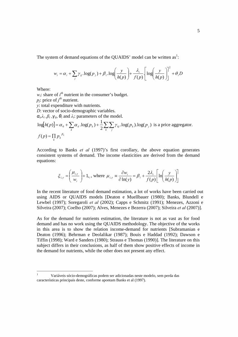
The system of demand equations of the QUAIDS’ model can be written as1:

Dph

ypfph

ypw ii

jijijii θ

λβγα +⎥

⎦

⎤⎢⎣

⎡⎟⎟⎠

⎞⎜⎜⎝

⎛+⎟⎟

⎠

⎞⎜⎜⎝

⎛++= ∑

2

)(log.

)()(log.)log(.

Where: wi: share of ith nutrient in the consumer’s budget. pj: price of jth nutrient. y: total expenditure with nutrients. D: vector of socio-demographic variables. αi,λi ,βi ,γij, θi and λi: parameters of the model.

[ ] ∑ ∑∑++=k k j

jkkjkk pppph )log().log(.21)log(.)(log 0 γαα is a price aggregator.

kk

kppf β∏=)(

According to Banks et al (1997)’s first corollary, the above equation generates consistent systems of demand. The income elasticities are derived from the demand equations:

ii

yiyi w

,1,, +⎟⎟

⎠

⎞⎜⎜⎝

⎛=

μξ , where ⎥

⎦

⎤⎢⎣

⎡⎟⎟⎠

⎞⎜⎜⎝

⎛+=

∂∂

≡)(

ln)(

2)ln(, ph

ypfy

w ii

iyi

λβμ

In the recent literature of food demand estimation, a lot of works have been carried out using AIDS or QUAIDS models [Deaton e Muellbauer (1980); Banks, Blundell e Lewbel (1997); Soregaroli et al (2002); Capps e Schmitz (1991); Menezes, Azzoni e Silveira (2007); Coelho (2007); Alves, Menezes e Bezerra (2007); Silveira et al (2007)]. As for the demand for nutrients estimation, the literature is not as vast as for food demand and has no work using the QUAIDS methodology. The objective of the works in this area is to show the relation income-demand for nutrients [Subramanian e Deaton (1996); Behrman e Deolalikar (1987); Bouis e Haddad (1992); Dawson e Tiffin (1998); Ward e Sanders (1980); Strauss e Thomas (1990)]. The literature on this subject differs in their conclusions, as half of them show positive effects of income in the demand for nutrients, while the other does not present any effect.

1 Variáveis sócio-demográficas podem ser adicionadas neste modelo, sem perda das características principais deste, conforme apontam Banks et al (1997).

6

3. DATA SET

The database used for estimation was from microdata of Brazilian Household Expenditure Survey (Pesquisa de Orçamentos Familiares from june-2002 to july-2003), elaborated by Brazilian Bureau of Statistics (Instituto Brasileiro de Geografia e Estatística – IBGE, 2004b). The data were analyzed as a cross-section of urban households. The nutrients’ choice was based on the relevance in Brazilian food dietary (by Ministry of Health in Brazil, ANVISA), which are: proteins; lipids; carbohydrates; fibers; cholesterol; calcium; sodium; iron; and vitamins A, B, and C The conversion of goods’ amount purchased into nutrients was made using well-known Brazilian tables of food composition [TACO-UNICAMP; TBCA-USP: ENDEF-IBGE and Philippi, 2002]. The price index used instead of the equation of price aggregator was the Stone price index, as for cross-section data this index is equivalent to the Paasche index, which is pointed out by Moschini (1995) as the best price index for the AIDS and QUAIDS’ model.

4. ESTIMATION

The demand equations were estimated by Full-Information Maximum Likelihood (FIML), which derives consistent estimations (Greene, 2003; Hayashi, 2000; Wooldridge, 2001), and the statistic software used was STATA/SE version 10.0. The results for Brazil were obtained assuming the theoretical hypothesis from the demand equations. The following table summarizes the results for all the demand equations, which are commented on the next section.

7

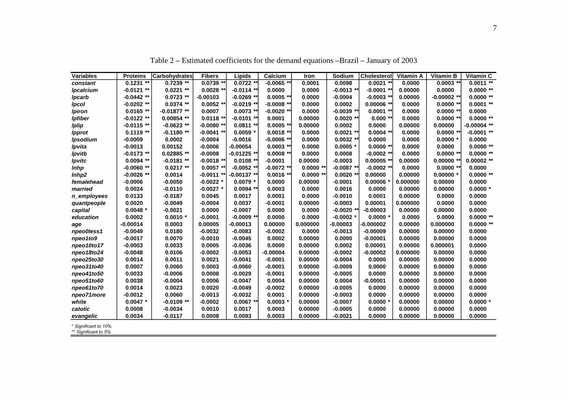
Table 2 – Estimated coefficients for the demand equations –Brazil – January of 2003

Variablesconstant 0.1231 ** 0.7239 ** 0.0739 ** 0.0722 ** -0.0065 ** 0.0001 0.0098 0.0021 ** 0.0000 0.0003 ** 0.0011 **lpcalcium -0.0121 ** 0.0221 ** 0.0028 ** -0.0114 ** 0.0000 0.0000 -0.0013 ** -0.0001 ** 0.00000 0.0000 0.0000 **lpcarb -0.0442 ** 0.0723 ** -0.00103 -0.0269 ** 0.0005 ** 0.0000 -0.0004 -0.0003 ** 0.00000 -0.00002 ** 0.0000 **lpcol -0.0202 ** 0.0374 ** 0.0052 ** -0.0219 ** -0.0008 ** 0.0000 0.0002 0.00006 ** 0.0000 0.0000 ** 0.0001 **lpiron 0.0165 ** -0.01877 ** 0.0007 0.0073 ** -0.0020 ** 0.0000 -0.0039 ** 0.0001 ** 0.0000 0.0000 ** 0.0000lpfiber -0.0122 ** 0.00854 ** 0.0118 ** -0.0101 ** 0.0001 0.00000 0.0020 ** 0.000 ** 0.0000 0.0000 ** 0.0000 **lplip -0.0115 ** -0.0623 ** -0.0080 ** 0.0811 ** 0.0005 ** 0.00000 0.0002 0.0000 0.00000 0.00000 -0.00004 **lpprot 0.1119 ** -0.1180 ** -0.0041 ** 0.0059 * 0.0018 ** 0.0000 0.0021 ** 0.0004 ** 0.0000 0.0000 ** -0.0001 **lpsodium -0.0009 0.0002 -0.0004 -0.0016 -0.0006 ** 0.0000 0.0032 ** 0.0000 0.0000 0.0000 * 0.0000lpvita -0.0013 0.00152 -0.0006 -0.00054 0.0003 ** 0.0000 0.0005 * 0.0000 ** 0.0000 0.0000 0.0000 **lpvitb -0.0173 ** 0.02885 ** -0.0008 -0.01225 ** 0.0008 ** 0.0000 0.0008 -0.0002 ** 0.0000 0.0000 ** 0.0000 **lpvitc 0.0094 ** -0.0181 ** -0.0018 ** 0.0108 ** -0.0001 0.00000 -0.0003 0.00005 ** 0.00000 0.00000 ** 0.00002 **lnhp -0.0060 ** 0.0217 ** 0.0057 ** -0.0052 ** -0.0072 ** 0.0000 ** -0.0087 ** -0.0002 ** 0.0000 0.0000 ** 0.0000lnhp2 -0.0026 ** 0.0014 -0.0011 ** -0.00137 ** 0.0016 ** 0.0000 ** 0.0020 ** 0.00000 0.00000 0.00000 * 0.0000 **femalehead -0.0006 -0.0050 -0.0022 * 0.0079 * 0.0000 0.00000 -0.0001 0.00006 * 0.000000 0.00000 0.0000married 0.0024 -0.0110 -0.0027 * 0.0094 ** 0.0003 0.0000 0.0016 0.0000 0.00000 0.00000 0.0000 *n_employees 0.0133 -0.0187 0.0045 0.0017 0.0001 0.0000 -0.0010 0.0001 0.00000 0.0000 0.0000quantpeople 0.0020 -0.0049 -0.0004 0.0037 -0.0001 0.00000 -0.0003 0.00001 0.000000 0.0000 0.0000capital 0.0048 * -0.0021 0.0000 -0.0007 0.0000 0.0000 -0.0020 ** -0.00003 0.00000 0.00000 0.0000education 0.0002 0.0010 * -0.0001 -0.0009 ** 0.0000 0.0000 -0.0002 * 0.0000 * 0.0000 0.0000 0.0000 **age -0.00014 0.0003 0.00005 -0.00013 0.00000 0.000000 -0.00003 -0.000002 0.00000 0.000000 0.0000 **npeo0less1 -0.0049 0.0180 -0.0032 -0.0083 -0.0002 0.0000 -0.0013 -0.00009 0.00000 0.00000 0.0000npeo1to9 -0.0017 0.0070 -0.0010 -0.0045 0.0002 0.00000 0.0000 -0.00001 0.00000 0.00000 0.0000npeo10to17 -0.0003 0.0033 0.0005 -0.0036 0.0000 0.00000 0.0002 0.00001 0.00000 0.000001 0.0000npeo18to24 -0.0048 0.0106 -0.0002 -0.0053 -0.00004 0.00000 -0.0002 -0.00002 0.000000 0.00000 0.0000npeo25to30 0.0014 0.0011 0.0021 -0.0041 -0.0001 0.00000 -0.0004 0.0000 0.00000 0.00000 0.0000npeo31to40 0.0007 0.0060 0.0003 -0.0060 -0.0001 0.00000 -0.0009 0.0000 0.00000 0.00000 0.0000npeo41to50 0.0033 -0.0006 0.0008 -0.0029 -0.0001 0.00000 -0.0005 0.0000 0.00000 0.00000 0.0000npeo51to60 0.0038 -0.0004 0.0006 -0.0047 0.0004 0.00000 0.0004 -0.00001 0.00000 0.00000 0.0000npeo61to70 0.0014 0.0023 0.0020 -0.0049 -0.0002 0.00000 -0.0005 0.0000 0.00000 0.00000 0.0000npeo71more -0.0012 0.0060 -0.0013 -0.0032 0.0001 0.00000 -0.0003 0.0000 0.00000 0.00000 0.0000white 0.0047 * -0.0109 ** -0.0002 0.0067 ** 0.0003 * 0.00000 -0.0007 0.0000 * 0.00000 0.00000 0.0000 *catolic 0.0008 -0.0034 0.0010 0.0017 0.0003 0.00000 -0.0005 0.0000 0.00000 0.00000 0.0000evangelic 0.0034 -0.0117 0.0008 0.0093 0.0003 0.00000 -0.0021 0.0000 0.00000 0.00000 0.0000

* Significant to 10%** Significant to 5%

Vitamin A Vitamin B Vitamin CCalcium Iron Sodium CholesterolProteins Carbohydrates Fibers Lipids

8

The description of the variables is: Dummies for characteristics: white; married; catholic; evangelic; female head; capital; and education; Discrete variables informing the numbers of occurrence: Number of members of the signed age (npeo0less1, npeo1to9, npeo10to17, npeo18to24, npeo25to30, npeo31to40, npeo41to50, npeo51to60, npeo61to70, and npeo71more); n_employees; and quantmor; Dependent variables: proteins; carbohydrates; fibers; lipids; calcium; iron; sodium; cholesterol; vitamin A; vitamin B; and vitamin C; Logarithm variables: price (lpcalcium, lpcarb, lpcol, lpiron, lpfiber, lplip, lpprot, lpsodium, lpvita, lpvitb, and lpvitc); expenditure (lnhp, and lnhp2)

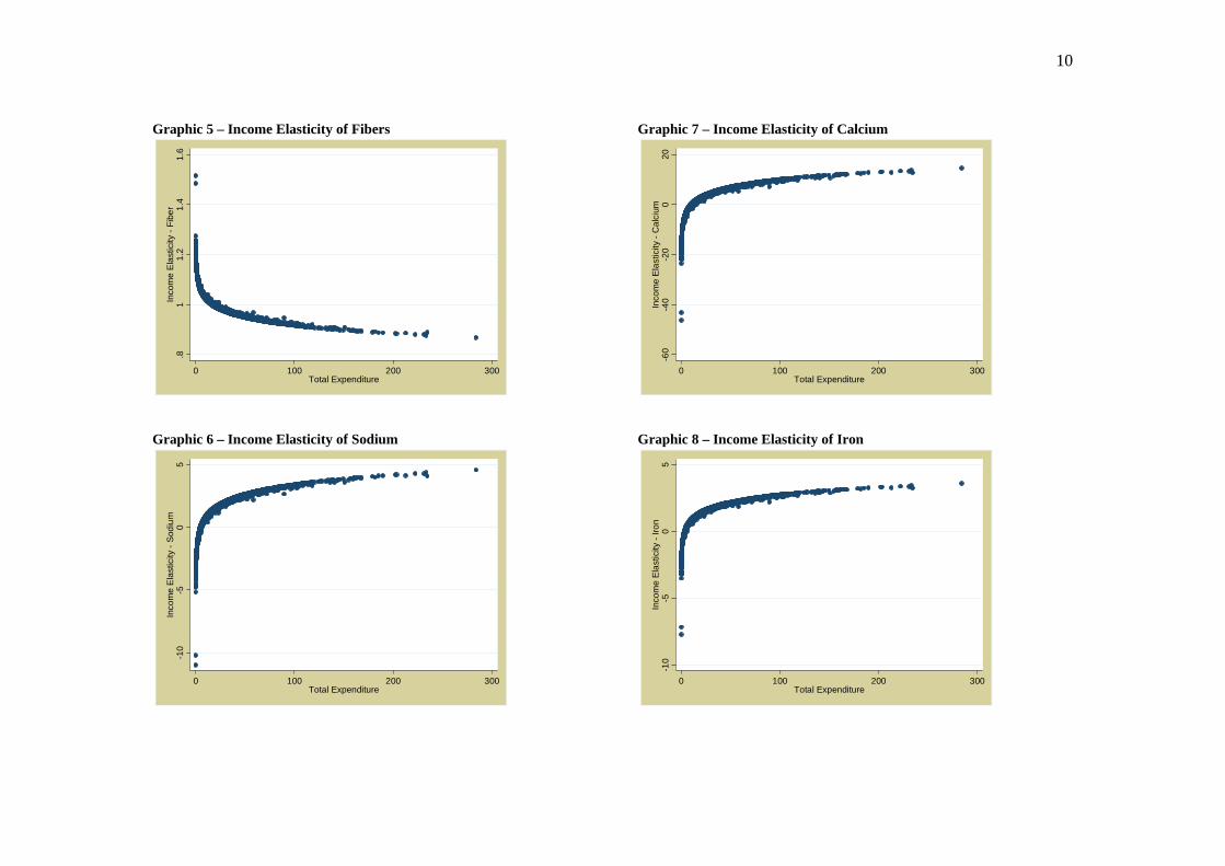
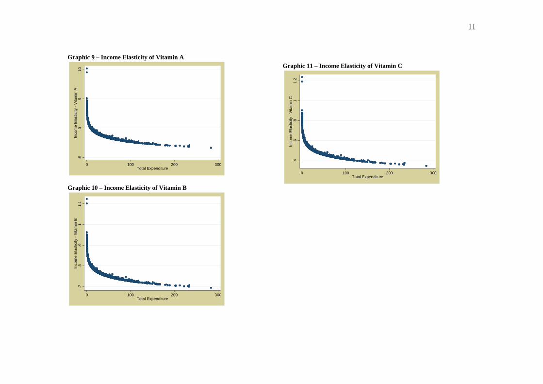
5. RESULTS AND CONCLUSIONS The results for socioeconomic variables indicated that households, where the meal planner is female, in comparison with male-headed households, demand more cholesterol and lipids, and less fiber. In addition to this result, households with married meal planners also consume more lipids and less fiber. The place of residence also showed differences of consumption. Capital located households presented, on average, more expenditure with protein; and less expenditure with sodium. Another interesting result is that white meal planners’ households demand more protein, vitamin C, lipids, calcium and cholesterol and less carbohydrate. The quadratic term of expenditure indicated that the nonlinearity of the Engel curve cannot be rejected for all the nutrients, except for carbohydrates, cholesterol, and vitamin A. The graphics of the expenditure elasticities of nutrients are presented below2:

2 The legend of the graphics is in Portuguese. The observations with exes are from the unrestricted model and the gray observations are results of the restricted model. The horizontal line indicates the total expenditure of the families.

9

Graphic 1 – Income Elasticity of Proteins

.8.9

11.

11.

2In

com

e E

last

icity

- P

rote

ins

0 100 200 300Total Expenditure

Graphic 2 – Income Elasticity of Carbohydrates

1.01

1.02

1.03

1.04

1.05

Inco

me

Ela

stic

ity -

Car

bohy

drat

es

0 100 200 300Total Expenditure

Graphic 3 – Income Elasticity of Lipids

.9.9

51

1.05

1.1

Inco

me

Elas

ticity

- Li

pids

0 100 200 300Total Expenditure

Graphic 4 – Income Elasticity of Cholesterol

.6.6

5.7

.75

.8In

com

e El

astic

ity -

Cho

lest

erol

0 100 200 300Total Expenditure

10

Graphic 5 – Income Elasticity of Fibers

.81

1.2

1.4

1.6

Inco

me

Elas

ticity

- Fi

ber

0 100 200 300Total Expenditure

Graphic 6 – Income Elasticity of Sodium

-10

-50

5In

com

e E

last

icity

- So

dium

0 100 200 300Total Expenditure

Graphic 7 – Income Elasticity of Calcium

-60

-40

-20

020

Inco

me

Ela

stic

ity -

Cal

cium

0 100 200 300Total Expenditure

Graphic 8 – Income Elasticity of Iron

-10

-50

5In

com

e El

astic

ity -

Iron

0 100 200 300Total Expenditure

11

Graphic 9 – Income Elasticity of Vitamin A

-50

510

Inco

me

Elas

ticity

- Vi

tam

in A

0 100 200 300Total Expenditure

Graphic 10 – Income Elasticity of Vitamin B

.7.8

.91

1.1

Inco

me

Ela

stic

ity -

Vita

min

B

0 100 200 300Total Expenditure

Graphic 11 – Income Elasticity of Vitamin C

.4.6

.81

1.2

Inco

me

Ela

stic

ity -

Vita

min

C

0 100 200 300Total Expenditure

12

The graphics above suggested the following behavior: - Protein, lipid and fiber: Luxury goods for low income households, and necessary goods for richer households; - Vitamins A, B and C: Inferior goods for most part of the households; - Carbohydrates and Cholesterol: Normal goods for all the income levels; - Calcium, sodium and iron: Inferior goods for low-income households, and luxury goods for high-income levels. For proteins, the observed pattern is in accordance with other works [Alves, Menezes and Bezerra (2007); Ward and Sanders (1980)], as the proteins’ consumption increases with income, due to the high-value of products rich in this nutrient. On the other hand, for Carbohydrates the results suggested that it is a nutrient highly consumed by Brazilian households, being a normal good for all income levels. it is believed that there exist changes in the type of this nutrient consumed by poor (rice and beans) and rich households (pasta, potato, vegetables and cereals). Lipids show the same pattern as proteins, which means that this nutrient is more consumed as income increases. These results are important to measure the improvement in nutrients intake, when income increase. It is possible to conclude that carbohydrates and cholesterol, for example, are inexpensive, and eaten most heavily by the poor. When it comes to fats and proteins, these nutrients are consumed in higher proportion by the rich, as it can be seen by the elasticity estimated. These evidences can be helpful for the design of specific public policies in order to bring benefits to the food diet of the Brazilian population One of the limitations of this paper is the endogeneity of the variable income in the demand equation, firstly pointed out by Stiglitz (1976). As the estimation by Non-linear SUR (or FIML) is computationally complicated, the treatment of this problem would be very difficult to account. Future research should try to correct a possible bias from this endogeneity.

6. REFERENCES

Alves, Denisard C. O, Menezes, Tatiane A. and Fernado Bezerra (2007), “Estimação do sistema de demanda censurada para o Brasil,” in Gasto e consumo das famílias brasileiras contemporâneas, Brasília: IPEA, v.2, 395-421. Banks, James, and Lewbel Blundell (1997), “Quadratic Engel Curves and Consumer Demand”, The Review of Economics and Statistics, Vol. 79, No. 4, 527-539.

13

Behrman, J. R., Deolalikar, A. B. (1989), “The Intrahousehold Demand for Nutrients in Rural South India: Individual Estimates, Fixed Effects, and Permanent Income”, The Journal of Human Resources, Vol. 25, No. 4, 665-696. Blundell, R., Pashardes, P., Weber, G. (1993), “What do we Learn About Consumer Demand Patterns from Micro Data?”, The American Economic Review, Vol. 83, No. 3, 570-597. Bouis, H. E., Haddad, L. J. (1992), “Are estimates of calorie-income elasticities too high? : A recalibration of the plausible range”, Journal of Development Economics, vol. 39, 333-364. Castro, Josué. (1980), Geografia da fome. Rio de Janeiro: Ed. Antares. Christensen, L., Jorgenson, D. e Lau, L. (1975), “Transcendental Logarithmic Utility Functions”, American Economic Review, vol. 65, 367-83. Coelho, A. B. (2006), A demanda de alimentos no Brasil, 2002/2003. PhD Dissertation, Universidade Federal de Viçosa. Cranfield, J.A.L., Eales, J.S., Hertel, T.W., and Preckel, P.V.(2003), “Model Selection when Estimating and Predicting Consumer Demands using International, Cross Section Data”, Empirical Economics 28(2), 353-364. Dawson, P. J. Tiffin, R. (1998), “Estimating the Demand for Calories in India”, American Journal of Agricultural Economics, Vol. 80, No. 3, 474-481. Deaton, A. and Muellbauer, J. (1980a), “Almost Ideal Demand System”, American Economic Review, vol. 70, 312-326. Deaton, A. and Muellbauer, J. (1980b), Economics and Consumer Behavior, Cambridge: Cambridge University Press, 3-147. Deaton, A. (1986), Handbooks of Econometrics. Chapter 30: Demand Analysis. Elsevier Science Publishers, BV,1768-1839. Greene, W. H. (2003), Econometric Analysis. New Jersey: Prentice Hall, 5th ed.. Hayashi, F. (2000), Econometrics. New Jersey: Princeton University Press, 529-537. IBGE (2004a), Pesquisa de Orçamentos Familiares 2002-2003: Primeiros Resultados Brasil e Grandes Regiões. Rio de Janeiro: Instituto Brasileiro de Geografia e Estatística. IBGE (2004b), Pesquisa de Orçamentos Familiares 2002-2003. CD-ROM - Microdados – Segunda divulgação. Rio de Janeiro: Instituto Brasileiro de Geografia e Estatística.

14

IBGE (2004c), Pesquisa de Orçamentos Familiares 2002-2003. Análise da Disponibilidade Domiciliar de Alimentos e do estudo nutricional no Brasil. Rio de Janeiro: Instituto Brasileiro de Geografia e Estatística e Ministério da Saúde. Klein, L. R. and Rubin, H. (1948), "A Constant Utility Index of the Cost of Living," Review of Economic Studies, No. 2, Vol. 15, p. 84-87. Lancaster, K. J. (1966) “A New approach to consumer theory. Journal of Political Economy”, n. 74, 132-157. Mas-Collel, A., Whinston, M. D. and Green, J. R. (1995), Microeconomic theory. Oxford: Oxford University Press. Menezes, T. A., Silveira, F. G. and Azzoni, C. R. (2007), “Demand elasticities for food products: a two-stage budgeting system”, Paper accepted for publication in Applied Economics. Moschini, G. (1995), “Units of Measurement and the Stone Index in Demand System Estimation”, American Journal of Agricultural Economics, Vol. 77, No. 1. , 63-68. MRE (1996), Relatório Nacional Brasileiro - Cúpula Mundial de Alimentação- Roma, Brasiília: MRE. Philippi, S. T. (2002), Tabela de composição de alimentos: suporte para decisão nutricional. Brasília: Coronário. Philips, L. (1974), Applied Consumption Analysis, New York: North Holland. Sichieri, R., Coitinho, D. C., and Monteiro, J. B. (2000), “Recomendações de Alimentação e Nutrição Saudável para a População Brasileira”, Arquivos Brasileiros de Endocrinologia e Metabolismo, vol.44, no.3, São Paulo. Silveira, F. G., Magalhães, L. C. G., Menezes, T. A., and Diniz, B. P. C. (2007), “Elasticidade-Renda dos Produtos Alimentares nas Regiões Metropolitanas Brasileiras: Uma Aplicação da POF 1995/1996”, Estudos Econômicos, São Paulo, V. 37, N.2, 329-352. Soregaroli, C., Huff, K., and Meilke, K. (2002), “Demand System Choice Based on Testing the Engel Curve Specification”, Working Paper 02/09, University of Guelph, Ontário. Subramanian, S. and Deaton, A. (1996), “The Demand for Food and Calories,” The Journal of Political Economy, Vol. 104, No. 1, 133-162. Stiglitz, J. E., (1976) “Efficiency Wage Hypothesis, Surplus Labour and the Distribution of Income in L.D.C.'s”, Oxford Economic Papers, vol 38,185-207. Strauss, J. and Thomas, D. (1998), “Health, Nutrition and Economic Development”, Journal of Economic Literature. vol. 36, 766-817.

15

Ward, J. O. and Sanders, J. H. (1980), “Nutritional Determinants and Migration in the Brazilian Northeast: A Case Study of Rural and Urban Ceará”, Economic Development and Cultural Change, Vol. 29, No. 1, 141-163. Wooldridge, J. M. (2001), Econometrics Analysis of Cross Section and Panel Data. The Massachusetts Institute of Technology Press. WHO/FAO (2002), Diet Nutrition and the prevention of chronic diseases. WHO technical report series 916. Report of a Joint WHO/FAO Expert Consultation, Geneva.