Dr. Mohamed Ouda Electrical Engineering Department

Islamic University of Gaza

2013

Antenna Theory

EELE 5445

Lecture 6: Dipole Antenna

The dipole and the monopole The dipole and the monopole are arguably the two most widely used

antennas across the UHF, VHF and lower-microwave bands.

Arrays of dipoles are commonly used as base-station antennas in

land-mobile systems.

The monopole and its variations are perhaps the most common

antennas for portable equipment, such as cellular telephones,

cordless telephones, automobiles, trains, etc.

It has attractive features such as simple construction, sufficiently

broadband characteristics for voice communication, small

dimensions at high frequencies.

An alternative to the monopole antenna for hand-held units is the

loop antenna, the microstrip patch antenna, the spiral antennas,

inverted-L and inverted-F antennas, and others. Dr. M Ouda 2

Small dipole

Assuming , The maximum phase error βR in that can

occur is

at θ=0

Reminder: A maximum total phase error of π/8 is acceptable

since it does not affect substantially the integral solution for the

vector potential A. The assumption is made here for

both, the amplitude and the phase factors in the kernel of the

VP integral.

Dr. M Ouda 3

The current is a triangular function of : 'z

Dr. M Ouda 4

The solution for A is simple when we assume that

Note that A is exactly one-half of the result obtained for A of an

infinitesimal dipole of the same length, if Im were the current

uniformly distributed along the dipole.

This is expected because we made the same approximation for R,

as in the case of the infinitesimal dipole with a constant current

distribution, and we integrated a triangular function along l, whose

average is

Therefore, we need not repeat all the calculations of the field

components, power and antenna parameters. We make use of our

knowledge of the infinitesimal dipole field.

Dr. M Ouda 5

The far-field components of the small dipole are simply half those

of the infinitesimal dipole:

The normalized field pattern is the same as that of the infinitesimal

dipole:

Dr. M Ouda 6

Dr. M Ouda 7

The beam solid angle:

The directivity

As expected, the directivity, the beam solid angle as well as the

effective aperture are the same as those of the infinitesimal dipole

because the normalized patterns of both dipoles are the same.

Dr. M Ouda 8

The radiated power is four times less than that of an infinitesimal

dipole of the same length and current because the far fields are

twice smaller in magnitude: I0= Im

Dr. M Ouda 9

As a result, the radiation resistance is also four times smaller than that

of the infinitesimal dipole:

Finite-length infinitesimally thin dipole

A good approximation of the current distribution along the

dipole’s length is the sinusoidal one:

It can be shown that the VP integral

has an analytical (closed form) solution, however, we follow a

standard approach used to calculate the far field for an arbitrary wire

antenna. Dr. M Ouda 10

The dipole is subdivided into a number of infinitesimal dipoles of

length dz'. Each such dipole produces the elementary far field as

Where and denotes the value of

the current element at z'. Using the far-zone approximations,

We obtain

Dr. M Ouda 11

Dr. M Ouda 12

The first factor is the element factor.

Which is the far field produced by an infinitesimal dipole of unit

current element .

The element factor is the same for any current element,

Іl=1(Axm) provided the angle θ is always associated with the

current axis.

The second factor

is the space factor (or pattern factor, array factor). The

pattern factor is dependent on the amplitude and phase

distribution of the current at the antenna (the source distribution

in space).

For the specific current distribution described in page 10, the

pattern factor is

The above integrals are solved having in mind that

The far field of the finite-length dipole is obtained as

Dr. M Ouda 13

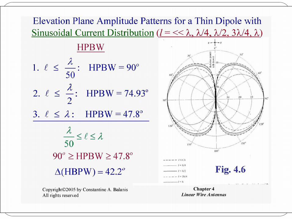
Amplitude pattern

Dr. M Ouda 14

Dr. M Ouda 16

Dr. M Ouda 17

Power pattern

Dr. M Ouda 18

Note: The maximum 𝐹 𝜃, 𝜑 of is not necessarily unity, but for

𝑙 < 2𝜆 the major maximum is always at 𝜃 = 900.

Radiated power First, the far-zone power flux density is calculated as

Dr. M Ouda 19

Dr. M Ouda 20

Radiation resistance

Dr. M Ouda 21

The radiation resistance is defined as

Therefore

Directivity

The directivity is obtained as

where the power pattern is

Finally

Dr. M Ouda 22

Input resistance

The radiation resistance given is not necessarily equal to the

input resistance because the current at the dipole center Iin (if its

center is the is not necessarily equal to Im. In particular,

𝐼𝑖𝑛 ≠ 𝐼𝑚 if l > λ/2, and 𝑙 ≠ 2(2𝑛 + 1)λ/2, n is any integer.

Note that when 𝑙 > λ, 𝐼𝑖𝑛 = 𝐼𝑚 .

To obtain a general expression for the current magnitude Iin at

the center of the dipole (assumed also to be a feed point), we

note that if the dipole is lossless, the input power is equal to the

radiated power. Therefore,

Dr. M Ouda 23

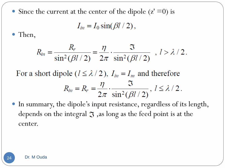
Since the current at the center of the dipole (z' =0) is

Then,

In summary, the dipole’s input resistance, regardless of its length,

depends on the integral ,as long as the feed point is at the

center.

Dr. M Ouda 24

Loss can be easily incorporated in the calculation of Rin bearing in

mind that the power-balance relation can be modified as

We have already obtained the expression for the loss of a dipole of

length l:

Dr. M Ouda 25

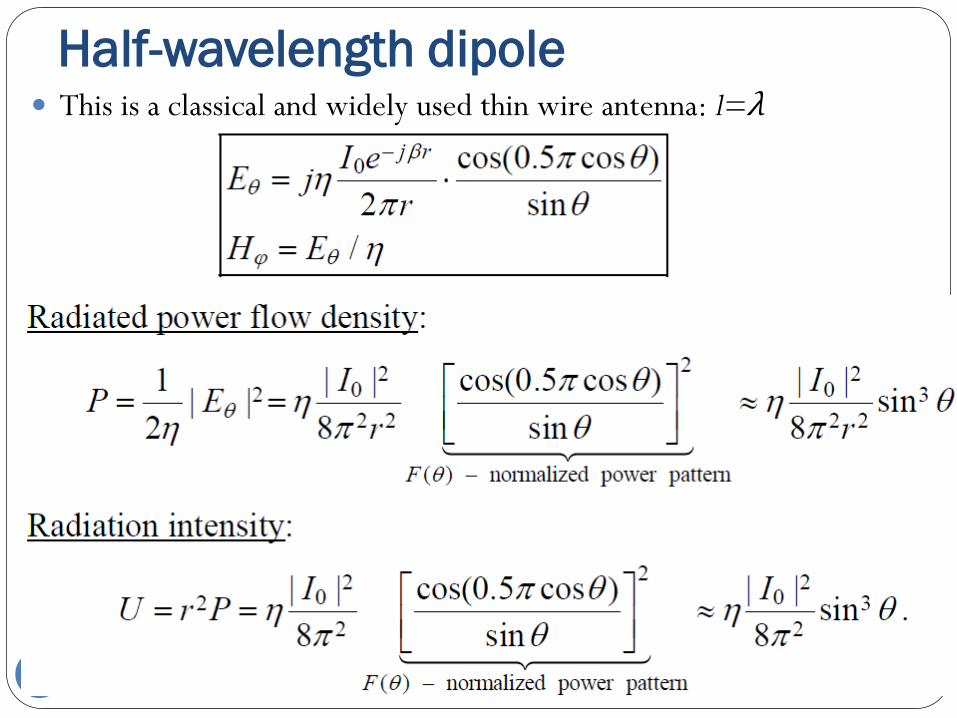
Half-wavelength dipole This is a classical and widely used thin wire antenna: l=λ

Dr. M Ouda 26

3-D power pattern (not in dB) of the half-wavelength dipole:

Dr. M Ouda 27

Radiated power

The radiated power of the half-wavelength dipole is a special

case of the integral in

Dr. M Ouda 28

Dr. M Ouda 29

The imaginary part of the input impedance is approximately

+j42.5Ω . To acquire maximum power transfer, this reactance has

to be removed by matching (e.g., shortening) the dipole:

thick dipole l≈0.47λ

thin dipole l ≈0.48λ

The input impedance of the dipole is very frequency sensitive;

i.e., it depends strongly on the ratio l/ λ . This is to be expected

from a resonant narrow-band structure operating at or near

resonance such as the half-wavelength dipole.

Also, the input impedance is influenced by the capacitance

associated with the physical junction to the transmission line. The

structure used to support the antenna, if any, can also influence

the input impedance. That is why the curves below describing the

antenna impedance are only representative. Dr. M Ouda 30

Measurement results for the input impedance of a dipole

Dr. M Ouda 31

Dr. M Ouda 32

Method of images – revision

Dr. M Ouda 33

Vertical electric current element

above perfect conductor

Dr. M Ouda 34

Using the total far field approximation and the VP integral

Dr. M Ouda 35

The total far field is

The far-field expression can be again decomposed into two

factors: the field of the elementary source g(θ) and the pattern

factor (also array factor) f(θ).

The normalized power pattern is

Dr. M Ouda 36

The elevation plane patterns for vertical infinitesimal electric dipoles

of different heights above a perfectly conducting plane are plotted :

Dr. M Ouda 37

As the vertical dipole moves further away from the infinite

conducting (ground) plane, more and more lobes are introduced in

the power pattern. This effect is called scalloping of the pattern. The

number of lobes is

Dr. M Ouda 38

Total radiated power

Dr. M Ouda 39

Note:

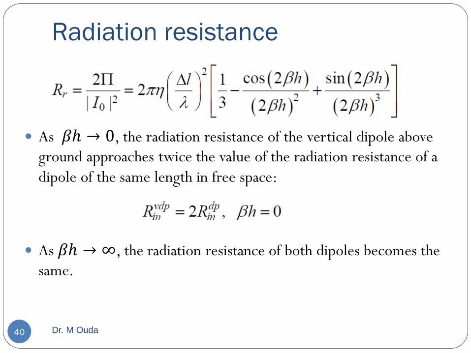
Radiation resistance

As 𝛽ℎ → 0, the radiation resistance of the vertical dipole above

ground approaches twice the value of the radiation resistance of a

dipole of the same length in free space:

As 𝛽ℎ → ∞, the radiation resistance of both dipoles becomes the

same.

Dr. M Ouda 40

Radiation intensity

The maximum of U(θ) occurs at θ=π/2:

This value is 4 times greater than of a free-space dipole of the same

length.

Dr. M Ouda 41

Maximum directivity

If 𝛽ℎ = 0, 𝐷𝑜 = 3, which is twice the maximum directivity of a

free-space current element (𝐷𝑖𝑑𝑜 =1.5 ).

The maximum of 𝐷𝑜 as a function of the height h occurs when

𝛽ℎ =2.881 (h=0.4585λ). Then, 𝐷𝑜=6.566/𝛽ℎ =2.881

Dr. M Ouda 42

Dr. M Ouda 43

Monopoles A monopole is a dipole that has been divided into half at its center

where it is fed against a ground plane. It is normally λ

4 long (a

quarter-wavelength monopole).

Dr. M Ouda 44

Dr. M Ouda 45

Several important conclusions follow from the image theory

The field distribution in the upper half-space is the same as that of

the respective free-space dipole.

The currents and charges on a monopole are the same as on the

upper half of its dipole counterpart but the terminal voltage is only

half that of the dipole. The input impedance of a monopole is

therefore only half that of the respective dipole:

The total radiated power of a monopole is half the power radiated by

its dipole counterpart since it radiates in half-space (but its field is

the same). As a result, the beam solid angle of the monopole is half

that of the respective dipole and its directivity is twice the directivity

of the dipole:

Dr. M Ouda 46

Dr. M Ouda 47

Some approximate formulas for rapid calculations of the input

resistance of a dipole and the respective monopole:

Dr. M Ouda 48

Horizontal current element above a

perfectly conducting plane

Dr. M Ouda 49

Where

Using the far field approximation

Dr. M Ouda 50

The fare field normalized pattern

Dr. M Ouda 51

As the height increases beyond a wavelength (h>λ), scalloping

appears with the number of lobes being

Dr. M Ouda 52

The radiated power and the radiation resistance

It is also obvious that if h=0, then Rr and Π=0 . This is to be

expected because the dipole is short-circuited by the ground plane.

Dr. M Ouda 53

Radiation Intensity

The maximum value depends on whether βh is less than π/2 or

greater:

Maximum directivity

For small βh

Dr. M Ouda 54