Anthropogenic radiative forcing time series from pre-industrialtimes until 2010
R. B. Skeie1, T. K. Berntsen1,2, G. Myhre1, K. Tanaka1,3, M. M. Kvalev ag1, and C. R. Hoyle3,*
1Center for International Climate and Environmental Research – Oslo (CICERO), Oslo, Norway2Department of Geosciences, University of Oslo, Oslo, Norway3Institute for Atmospheric and Climate Science, ETH Zurich, Zurich, Switzerland* now at: Laboratory of Atmospheric Chemistry, Paul Scherrer Institut, Villigen, Switzerland
Received: 10 June 2011 – Published in Atmos. Chem. Phys. Discuss.: 10 August 2011Revised: 11 November 2011 – Accepted: 14 November 2011 – Published: 29 November 2011
Abstract. In order to use knowledge of past climate changeto improve our understanding of the sensitivity of the climatesystem, detailed knowledge about the time development ofradiative forcing (RF) of the earth atmosphere system is cru-cial. In this study, time series of anthropogenic forcing ofclimate from pre-industrial times until 2010, for all well es-tablished forcing agents, are estimated. This includes presen-tation of RF histories of well mixed greenhouse gases, tro-pospheric ozone, direct- and indirect aerosol effects, surfacealbedo changes, stratospheric ozone and stratospheric watervapour. For long lived greenhouse gases, standard methodsare used for calculating RF, based on global mean concentra-tion changes. For short lived climate forcers, detailed chem-ical transport modelling and radiative transfer modelling us-ing historical emission inventories is performed. For the di-rect aerosol effect, sulphate, black carbon, organic carbon,nitrate and secondary organic aerosols are considered. Foraerosol indirect effects, time series of both the cloud lifetimeeffect and the cloud albedo effect are presented. Radiativeforcing time series due to surface albedo changes are calcu-lated based on prescribed changes in land use and radiativetransfer modelling. For the stratospheric components, simplescaling methods are used. Long lived greenhouse gases (LL-GHGs) are the most important radiative forcing agent witha RF of 2.83±0.28 W m−2 in year 2010 relative to 1750.The two main aerosol components contributing to the directaerosol effect are black carbon and sulphate, but their contri-butions are of opposite sign. The total direct aerosol effect
was−0.48±0.32 W m−2 in year 2010. Since pre-industrialtimes the positive RF (LLGHGs and tropospheric O3) hasbeen offset mainly by the direct and indirect aerosol effects,especially in the second half of the 20th century, which pos-sibly lead to a decrease in the total anthropogenic RF in themiddle of the century. We find a total anthropogenic RF inyear 2010 of 1.4 W m−2. However, the uncertainties in thenegative RF from aerosols are large, especially for the cloudlifetime effect.
1 Introduction
Since the industrial revolution, anthropogenic activities havealtered the concentrations of components in the atmosphere,some of which impact the radiative balance of the earth sys-tem. Long-lived greenhouse gases, primarily carbon diox-ide (CO2) but also methane (CH4), nitrous oxide (N2O) andhalocarbons are the most important anthropogenic climateforcing agents (Forster et al., 2007), but short lived com-ponents like tropospheric ozone and black carbon aerosolscause also a significant heating of the climate system. Sul-phate, organic carbon and nitrate form short lived aerosolsthat scatter solar radiation and thus lead to a cooling of theclimate system through the direct aerosol effect. In addi-tion, the aerosols can alter the cloud properties, causing indi-rect aerosol effects (Twomey, 1977; Albrecht, 1989). Also,changes in stratospheric water vapour and ozone in the strato-sphere as well as anthropogenic changes to the properties ofthe land surface give a radiative forcing on the climate system(Forster et al., 2007).
Published by Copernicus Publications on behalf of the European Geosciences Union.
11828 R. B. Skeie et al.: Anthropogenic radiative forcing time series
In order to understand recent climate change, knowing theradiative forcing time series for climate forcers is important.Not only radiative forcing at the present time, relative to thepre-industrial era, as is often presented in radiative forcingstudies (e.g Gauss et al., 2006; Schulz et al., 2006), is of in-terest, but also how the radiative forcing has developed overtime (Myhre et al., 2001; Takemura et al., 2006; Hansen etal., 2007). Also for future climate change, knowledge ofwhat has happened in the past is important. Climate sensitiv-ity, the equilibrium surface temperature change following adoubling of the CO2 concentration, is a highly uncertain butvery important parameter for future climate change predic-tion (Knutti and Hegerl, 2008). To constrain the climate sen-sitivity, based on simple climate models and observed tem-perature change, knowledge of the historical development inthe total radiative forcing is crucial (Tanaka et al., 2009).
In this study, we present time series of the radiative forc-ing, from pre-industrial times until 2010, for the main an-thropogenic components which influence climate. The con-centration increases of well mixed greenhouse gases sincepre-industrial times are well known from ice core drilling(e.g. MacFarling Meure et al., 2006) and in situ observations,from which RF time series can be calculated. For short livedcomponents, there is a lack of spatial and temporal coveragein observations. Based on surface radiation measurements, adecrease of solar radiation from the early 1960s up to the late1980s was found (Ohmura and Lang, 1989), and at the end ofthe 20th century a surface solar brightening at numerous sta-tions in Europe and the United States was observed (Wild etal., 2005, 2009), related to a decline in anthropogenic emis-sions of short lived aerosols and aerosol precursors. Histor-ical emission inventories show that there has been a spatialshift in the distribution of emissions. For example, sulphurdioxide emissions peaked in Europe and North America inthe 1970s, while emissions in Eastern Asia continuously in-creased over the 20th century (Smith et al., 2011). For car-bonaceous aerosols emitted from fossil fuel and biofuel com-bustion, a similar pattern is found, with the industrializedcountries having a large share of the emissions in the firstpart of the 20th century and the developing countries a largershare at the end of the century (Bond et al., 2007).
The main focus of this work is on the short lived compo-nents, tropospheric ozone and aerosols. The anthropogenicaerosols included are sulphate, primary organic carbon andblack carbon of both fossil fuel and biomass burning origin,secondary organic aerosols and nitrate. Due to their short at-mospheric lifetime, the changes in the geographical patternof the emissions change the geographical distribution of thecomponents. Since the RF depends significantly on location,and there is significant co-variance with clouds and humid-ity, detailed atmospheric chemistry and aerosol modellingare needed to calculate RF for the short lived species. Weuse a chemical transport model (CTM) to calculate the con-centration changes of aerosols and tropospheric ozone dueto anthropogenic activities and a radiative transfer model for
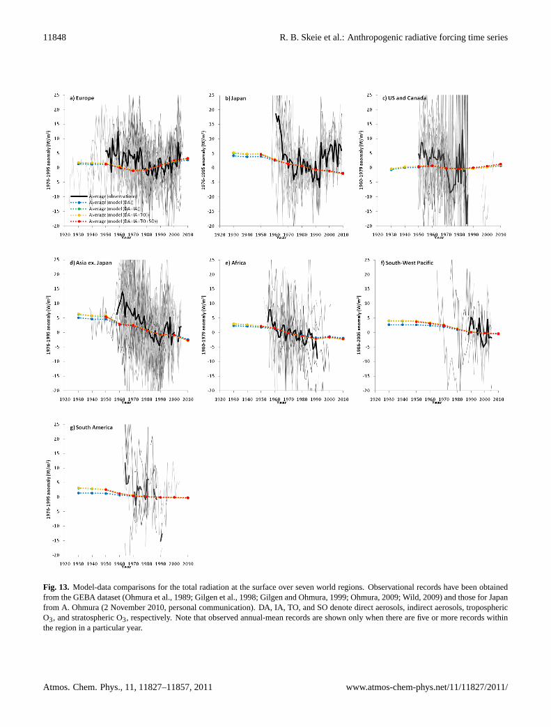
calculating RF time series. The historical emission inventoryof Lamarque et al. (2010) is used, which is also used in thehistorical CMIP5 (Coupled Model Intercomparison ProjectPhase 5) simulations for IPCC fifth assessment report.
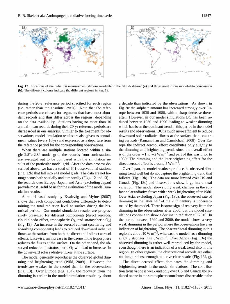
We present radiative forcing time series due to anthro-pogenic activities from pre-industrial times until present.Compared to previous works (Myhre et al., 2001; Takemuraet al., 2006; Hansen et al., 2007) the RF time series of shortlived climate components are based on revised emission in-ventories (Lamarque et al., 2010), detailed modelling by aCTM and radiative transfer modelling, and the time periodconsidered is extended to 2010. The paper is organized asfollows. In Sect. 2 the methods used for calculating theRF trends are described and in Sect. 3 the results and RFtime series are presented. At the end of Sect. 3 the simu-lated changes in radiation in different regions of the worldare compared with the observed global radiation compiled inthe Global Energy Balance Archive (GEBA). In Sect. 4 theresults are discussed and the summary and conclusions aregiven in Sect. 5.
2 Methods
In this section the methods used for calculating the radiativeforcing time series are described.
2.1 Long lived greenhouse gases
The radiative forcing time series for the long lived green-house gases (LLGHG) is calculated based on simplified ex-pressions from Myhre et al. (1998) and IPCC 2001 (Ra-maswamy et al., 2001), using historical concentrations basedon observational data as input. For halocarbons we use theupdated radiative efficiencies given in Table 2.14 in IPCC2007 (Forster et al., 2007). The time series of the LLGHGconcentrations from 1850 until 2010 are downloaded fromhttp://data.giss.nasa.gov/modelforce/ghgases/(Hansen et al.,1998; Hansen and Sato, 2004). These concentration series(GISS data) are based on ice core data and in situ measure-ments. The concentration time series are extended back-wards from 1850 to 1750 using ice core data from Etheridgeet al. (1996) for CO2 and from Etheridge et al. (1998) forCH4 (the same ice core data as used in the GISS data),which were reproduced by a more recent study from Mac-Farling Meure et al. (2006). For N2O, MacFarling Meureet al. (2006) found lower pre-industrial concentrations thanwhat is specified in the GISS data (Machida et al., 1995).The two ice cores have similar N2O concentrations back to1900. We have used the MacFarling Meure et al. (2006) datafrom 1900 and back to 1750.
2.2 Tropospheric ozone and aerosols
The OsloCTM2 model was used for calculating the con-centration changes of tropospheric ozone (O3) and aerosols.
R. B. Skeie et al.: Anthropogenic radiative forcing time series 11829
Table 1. Emissions used in this study. For each year and component the annual total anthropogenic and biomass burning emissions are listed.The natural emissions are presented in the bottom line. The year with maximum emissions are marked with a star (∗).
SOA precursors:
CO NMHC NOx NH3 SO2+SO4 DMS FFBF BC BC BB FFBF OC OC BB Isoprene Bio. VOC Ant. VOC(Tg) (Tg) (Tg N) (Tg N) (Tg S) (Tg) (Tg) (Tg) (Tg) (Tg) (Tg) (Tg C) (Tg)
Time slice simulations are done for 1850, 1900 and there-after every 10th year until 2010. Each time slice simula-tion is one year long and meteorological data for the year2006 are used. Each simulation is initialized by the samepre-industrial model climatology and a three year spin up isused. Anthropogenic and biomass burning historical emis-sion data are from Lamarque et al. (2010). For year 2010anthropogenic emissions from the Representative Concentra-tion Pathways scenario RCP4.5 (Thomson et al., 2011) areused, which are consistent with the historical emission data(Lamarque et al., 2010). For biomass burning we have usedthe year 2000 emissions for 2010. In addition, a simulationwith pre-industrial emissions has been performed. We usethe 1850s emissions from Lamarque et al. (2010) as a basis,switching off all sectors except agriculture, agriculture- andwaste burning and the domestic sector, which are reducedto 20 % of the 1850 emissions. This is a larger reductionin emission than scaling with∼60 % based on global pop-ulation growth estimated by Goldewijk (2005). However, asimple scaling factor related to global population does notcapture growth in emissions per capita between 1750 and1850 due to technology improvements, migration and land-use change and we have therefore used a lower factor. Forthe biomass burning, the emissions are assumed to be half ofthe 1850s emissions, which is consistent with the total pre-industrial emission data from Dentener (2006b). The totalannual emissions are presented in Table 1.
The natural emissions (Table 1) are assumed to be con-stant throughout the simulation period to separate the an-thropogenic contribution. The lightning emissions are basedon Price et al. (1997) scaled to 5 Tg N yr−1 and distributedover the year by convection activity data. The natural emis-sions of CO, NOx, and hydrocarbons from vegetation, oceanand soil are from the POET emission inventories (Granier et
al., 2005). The isoprene and biogenic volatile organic com-pounds (VOCs) important in SOA formation are as used inHoyle et al. (2009). The natural emissions of sulphur speciesare as described in Berglen et al. (2004) except that we usethe parameterizations of the DMS flux from Nightingale etal. (2000) and emission from continuous degassing volca-noes from Dentener et al. (2006b).
OsloCTM2 is an off-line atmospheric chemistry transportmodel, driven by meteorological data generated by the Inte-grated Forecast System (IFS) model at the European Centrefor Medium-Range Weather Forecasts (ECMWF). The reso-lution of the model used in this study is T42, (approximately2.8◦
×2.8◦) with 60 vertical layers ranging from the surfaceup to 0.1 hPa. In this study we include the troposphericchemistry scheme (Berntsen and Isaksen, 1997; Dalsøren etal., 2010), as well as modules for sulphate, nitrate, blackcarbon, primary organic carbon, secondary organic aerosols,mineral dust and sea salt.
The sulphur chemistry scheme is coupled with the oxidantchemistry (Berglen et al., 2004). For black carbon (BC) andprimary organic carbon (OC), a simple bulk scheme is used(Berntsen et al., 2006; Rypdal et al., 2009; Skeie et al., 2011),with the aging time dependent on season and latitude (Skeieet al., 2011). We treat OC and BC from fossil fuel and bio-fuel (FFBF) and biomass burning (BB) separately. Time se-ries of RF for FFBF BC are presented in Skeie et al. (2011),and therefore we do not focus on FFBF BC in this study.We also include a scheme for secondary organic aerosols(SOA), where secondary organic aerosols are formed by con-densation of the oxidation products of hydrocarbons (Hoyleet al., 2007). We allow the semi-volatile species to partitionto ammonium sulphate aerosols as well as existing organicaerosols. For nitrate, a thermodynamical model for treat-ment of gas/aerosol partitioning of semi-volatile inorganic
11830 R. B. Skeie et al.: Anthropogenic radiative forcing time series
aerosols is used based on the EQUSAM model (Metzger etal., 2002). Chemical equilibrium between inorganic com-pounds is simulated, including sea salt. The nitrate moduleused is described in Myhre et al. (2006) and the sea salt mod-ule in Grini et al. (2002). Nitrate is separated in a coarseand a fine mode, for separating the radiative properties of thenitrate aerosols. In the OsloCTM2, the mineral dust emis-sions are driven by wind (Grini et al., 2005), and we do notinclude anthropogenic changes to the soil erodibility, so nochanges in the dust emissions are assumed for the historicaltime period in this study. In the stratosphere monthly modelclimatological values of ozone and nitrogen species are used,except in the 3 lowermost layers in the stratosphere (approx-imately 2.5 km) where the tropospheric chemistry scheme isapplied to account for photochemical O3 production in thelower stratosphere due to emissions of NOx, CO and VOCs.
The chemistry module has been evaluated in Søvde etal. (2008; 2011), references above, as well as in multi modelstudies (Dentener et al., 2006a; Gauss et al., 2006; Shindellet al., 2006b; Stevenson et al., 2006; Fiore et al., 2009). Re-mark that changes in the model have been included sincethese multi model studies were preformed where OsloCTM2overestimated O3 in the tropics. The model has been in-volved in the AeroCom aerosol multi model comparisonproject (Kinne et al., 2006; Schulz et al., 2006; Textor etal., 2006), and the aerosol module has been validated againstin situ measurements and remote sensing data (Myhre et al.,2009). Myhre et al. (2009) found that the mean pattern ofaerosol optical depth from the model is broadly similar to theAERONET network of ground-based sun photometers andsatellite retrievals.
The optical properties for the direct aerosol effect simula-tions are described in Myhre et al. (2007a). Radiative forc-ing is calculated for the concentration changes by adoptingthe DISORT radiative transfer model (Stamnes et al., 1988;Myhre et al., 2007a) in offline calculations. The radiativetransfer simulations are performed with 8 streams. The me-teorological data including the cloud data are the same asused in OsloCTM2. For tropospheric O3 a broadband codefor long wave radiation and the DISORT code for short waveradiation is used (Myhre et al., 2000).
The cloud albedo effect has been simulated using the ap-proach from Quaas et al. (2006). They established a re-lationship between the concentration of cloud droplets andaerosols based on Moderate Resolution Imaging Spectrora-diometer (MODIS) data. All hydrophilic aerosols, includingnatural aerosols such as sub-micron size sea salt, sulphate,nitrate, primary and secondary organic aerosols are includedin this approach. The changes in the concentration of clouddroplets alter the cloud effective radius and thus the opticalproperties of the clouds. The radiative forcing is calculatedusing the same radiative transfer model as described above.This approach for the cloud albedo effect is restricted to wa-ter clouds.
For the cloud lifetime effect, the RF time series is createdin a simple way by scaling the best estimate of the current RFgiven in the review by Isaksen et al. (2009) who established,based on published estimates using models and satellite data,a best estimate and an uncertainty range for the cloud life-time effect in 2007 relative to pre-industrial times. The cloudlifetime effect is scaled back in time using the RF time se-ries for the cloud albedo effect. Rotstayn and Penner (2001)find, in a GCM study, that the magnitude and spatial distri-bution of the cloud albedo effect and cloud lifetime effectwere similar. This indicates that both processes are governedby the change in aerosol concentrations without any strongnon-linear effects and thus that a simple linear scaling is areasonable approach.
2.3 Stratospheric forcing agents
Due to the increase in ozone depleting components, strato-spheric O3 has decreased over the latter part of 20th cen-tury (Douglass et al., 2011). Time slice simulations withOsloCTM2 including stratospheric chemistry were not per-formed. Søvde et al. (2011) performed simulations ofstratospheric O3 in the year 2000, relative to 1850, usingOsloCTM2 including stratospheric chemistry. The resultingRF estimates were separated for source and source regions.Estimates were separated for changes in ozone due to tro-pospheric O3 precursors and changes in ozone due to chlo-rine and bromine components. The estimates were also sep-arated for ozone changes occurring in the troposphere andfor changes occurring in the stratosphere. The estimatedRF due to chlorine and bromine, was−0.20 W m−2 in thestratosphere and−0.06 W m−2 in the troposphere. We scalethis total RF from chlorine and bromine (−0.26 W m−2) witha time series of equivalent effective stratospheric chlorine(EESC) (Daniel and Velders, 2007) which we will call strato-spheric O3 RF. So in this study we separate the RF of ozonedue to emissions of ozone depleting components, labelledstratospheric O3 RF, and RF due to emissions of ozone pre-cursors, labelled tropospheric O3 RF, even if the changes arenot restricted to the troposphere or stratosphere. The scalingof EESC with a present day RF is a simple approach to con-struct the RF time series assuming linearity of stratosphericO3 RF. Forster and Shine (1997) investigated the linearity ofstratospheric O3 forcing, and found the RF was quite linear,within 7 %, with the magnitude of the ozone depletion.
The increased amount of CH4 in the stratosphere will in-crease stratospheric water vapour (H2O) when it is oxidised.Due to the low amount of water vapour in the stratosphere,and water vapour being a strong greenhouse gas, this willgive a RF. The RF of stratospheric water vapour for 2005relative to pre-industrial times given in the IPCC 2007 was0.07±0.05 W m−2, 15 % of the methane forcing (Forster etal., 2007). To construct a RF time series of H2O in thestratosphere we make a simple assumption assuming a lin-ear relationship between the CH4 RF and stratospheric H2O
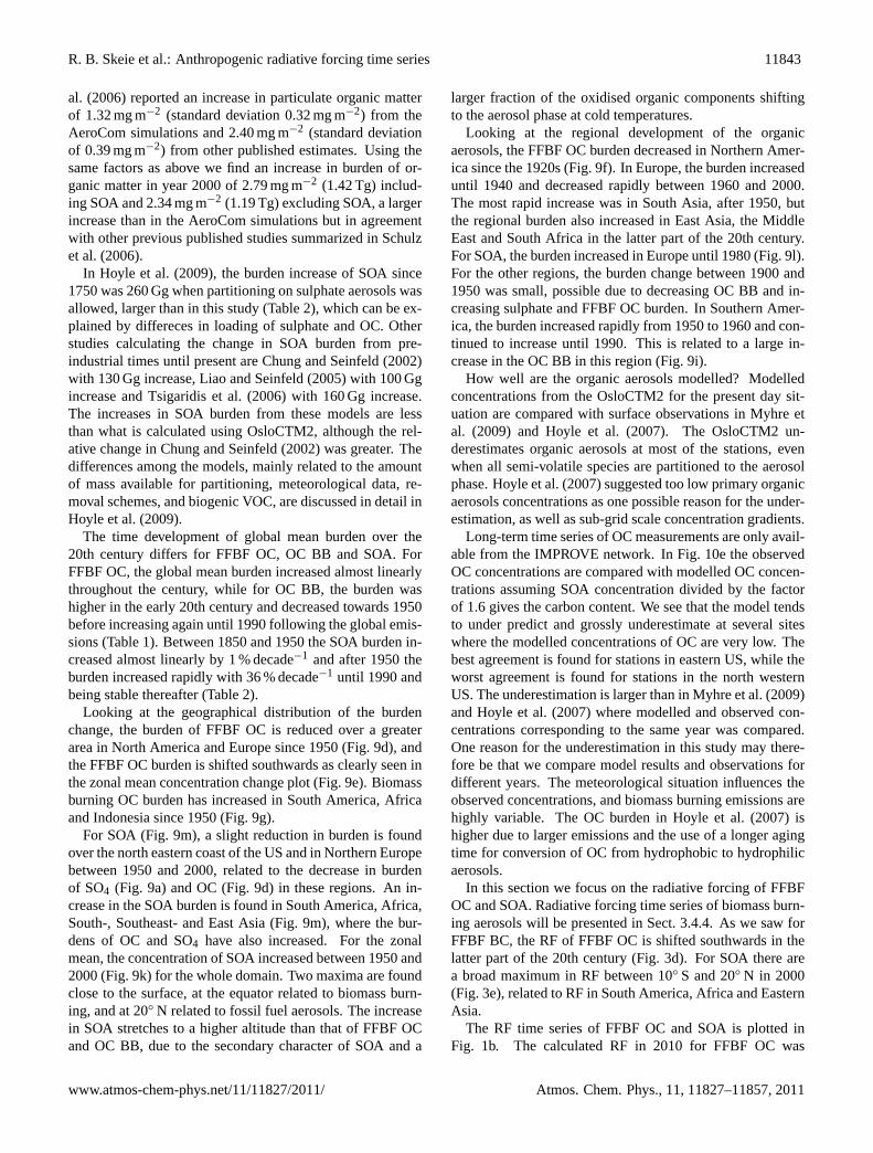
Figure 1: Time series of radiative forcing from 1850 until 2010 for the LLGHGs(a), the direct aerosol effect (b), all anthropogenic forcing mechanisms (c) andRF in 2010 for all components (d). The error bars represent the 90% confidenceinterval.
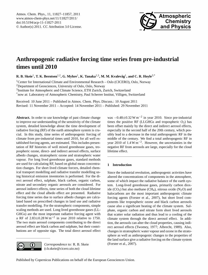
Fig. 1. Time series of radiative forcing from 1850 until 2010 for the LLGHGs(a), the direct aerosol effect(b), all anthropogenic forcingmechanisms(c) and RF in 2010 for all components(d). The error bars represent the 90 % confidence interval.
RF. For stratospheric H2O RF due to CH4 oxidation Myhreet al. (2007b) made explicit calculations for 1950, 1979 and2000 and the results were relatively linear with CH4 forcing.Remark that the time series presented here do not includedynamical causes for stratospheric H2O, only forcing due toCH4 oxidation. To construct a RF time series of H2O in thestratosphere, we therefore scale the CH4 RF time series with15 %.
2.4 Surface albedo changes
The radiative forcing due to land use change is associatedwith the change in surface albedo due to deforestation foragricultural purposes. We use global data sets of croplandfrom 1750–2005 (from the updated dataset atwww.geog.mcgill.ca/landuse/pub/Data/Histlanduse/on the basis of Ra-mankutty and Foley (1999)) to prescribe changes in croplandduring the industrial era. Surface albedo values are providedfor 16 vegetation types (Loveland et al., 2000). We haveadopted snow free surface albedo values in the visible and
near infrared, calculated using the MODIS albedo productMOD43B3 (Zhou et al., 2003; Gao et al., 2005). Land usechange also influences the hydrological cycle by altering i.e.runoff, evapotranspiration and precipitation (Kvalevag et al.,2010). These climate effects are considered as climate feed-back mechanisms and are not included in this study.
Snow albedo values are calculated using the method inBetts (2000) which includes snow cover, snow depth and amaximum snow albedo values for each vegetation type. Themaximum snow albedo values are latitude-average snow cov-ered surface albedo retrieved by MODIS (Gao et al., 2005).We also consider the zenith angle dependent surface albedofor snow free conditions using the approach from Hou etal. (2002) where the zenith angle dependency is either strongor weak for different vegetation types, and typically strongfor cropland. For snow covered vegetation we use the zenithangle dependency method introduced by Briegleb (1992)which uses a constant surface albedo for zenith angles below60 degrees but varies for zenith angles above 60 degrees.
11832 R. B. Skeie et al.: Anthropogenic radiative forcing time series
The atmospheric radiative transfer model used to studyland use change is the same as the one used for RF calcu-lations of ozone and aerosols.
The RF time series of the snow albedo effect due to blackcarbon deposited on snow are taken from Skeie et al. (2011).
3 Results
In this section we present radiative forcing time series from1750 to 2010. Unless otherwise stated all RF values pre-sented are relative to year 1750. The long-lived greenhousegases are first presented and then the tropospheric O3 results,before the stratospheric components (O3 and H2O). Thenwe concentrate on each of the aerosol components, sulphate(SO4), organic aerosols (OC+SOA), BC, biomass burningaerosols and nitrate, before presenting the total direct aerosoleffect and the indirect aerosol effects. Thereafter, radiativeforcing caused by surface albedo changes is presented. Fi-nally, the model results are compared with surface radiationobservations from the GEBA database. The time series foreach forcing component are plotted in Fig. 1 together withRF estimate for 2010 with an error bar indicating 90 % con-fidence interval (Fig. 1d).
3.1 Long-lived greenhouse gases
The calculated radiative forcing time series of CO2, CH4,N2O and other LLGHGs (CFCs, HCFCs, HFCs, PFCs andSF6) are presented in Fig. 1a. The RF of CO2 has increasedalmost continuously over the whole time period except forone period around 1940–1950 the reason of which is still un-der debate (Trudinger et al., 2002; MacFarling Meure et al.,2006; Rafelski et al., 2009). The RF of CO2 has increasedrapidly since 1950, from 0.62 W m−2 to 1.82 W m−2 in 2010.Over the last five years, the CO2 RF increased by 8.1 %. TheRF of CH4 has flattened out over the last decades, with avalue of 0.49 W m−2 in 2010. However, a renewed increasein the CH4 concentrations in the last couple of years hasbeen observed (Rigby et al., 2008). The forcing of N2O in-creased gradually since the beginning of 20th century, reach-ing 0.17 W m−2 in 2010. Over the last decades, the level ofRF of other LLGHGs flattened out, due to the reduction ofthe emissions of components covered by the Montreal Proto-col (Montzka et al., 2011b). In 2010 the RF of other LLGHGis estimated to be 0.34 W m−2.
The total RF of LLGHGs is plotted in Fig. 1c. Thetotal RF of LLGHGs in 2010 is 2.83 W m−2 (Fig. 1d) ofwhich CO2 contributed 64 %. The RF of LLGHGs has in-creased by 0.17 W m−2 over the last 5 yr. Compared toForster et al. (2007) the RF estimate of LLGHGs in 2005 is0.03 W m−2 (1.1 %) larger in this study, mainly due to 1ppmsmaller pre-industrial concentrations of CO2 in this study.The error bar added for this component has the same rela-tive uncertainty of 10 % as in Forster et al. (2007), which
includes the uncertainties in the RF calculations from con-centration changes and uncertainties in the measured concen-trations levels, especially the pre-industrial concentrations.The uncertainty in the measured CO2 concentration todayis less than 0.15 ppm and for pre-industrial concentrationsthe uncertainty is 1.2 ppm (Forster et al., 2007). The pre-industrial values used in our calculations of radiative forcingare 277 ppm for CO2, 710 ppb for CH4 and 271 ppb for N2O,while most of the halocarbons are of anthropogenic originand have therefore no pre-industrial concentration. The RFtime series are based on observed concentration changes, andmight therefore include geo-chemical feedbacks.
3.2 Tropospheric ozone and oxidation capacity
Ozone is produced in the troposphere by oxidation of carbonmonoxide (CO), methane (CH4) and non methane hydrocar-bons (NMHC) in presence of nitrogen oxides (NOx = NO+ NO2) and sunlight. The anthropogenic emissions of theseozone precursors have changed over the industrialized period(Table 1), and modelling studies show an increase in tropo-spheric O3 and thus a positive RF (e.g. Berntsen et al., 2000;Lamarque et al., 2005; Shindell et al., 2006a). Observationalstudies have also shown increase in tropospheric ozone (Lo-gan, 1994; Staehelin et al., 1994; Logan et al., 1999; Oltmanset al., 2006; Derwent et al., 2007).
3.2.1 Tropospheric ozone
The time series of the calculated RF from O3 is presented inFig. 1c, showing a steep increase in the decades following the1950s, and flattening out over the last decades. This resultsin a RF in 2010 of 0.44 W m−2 (Fig. 1d), corresponding to24 % of the CO2 forcing.
In Table 2, the global mean tropospheric burden changesince 1750 is presented. The largest increase is found be-tween 1950 and 1980 with a 42 % of the total increase inO3 burden. The total increase is 9.9 DU in 2000 com-pared to 1850, in line with the range of 7.9 DU to 13.8 DUfrom the multi model study by Gauss et al. (2006) and the9 DU increase between 1850 and 2000 found by Lamarqueet al. (2010), who used the same emission inventories as inthis study. The total increase between 1750 and 2010 in thisstudy is 11.4 DU.
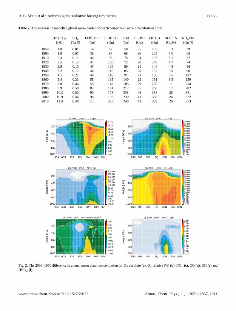
Most of the burden change occurred after 1950 (Table 2),and in Fig. 2a and b the absolute and relative differencesin the annual zonal mean O3 between 1950 and 2000 areshown. The largest increase is found in the Northern Hemi-sphere (NH), where the ozone precursor changes are largest(Fig. 2c–d), and the largest relative increase in ozone is foundat the surface in the NH (Fig. 2b). For NOx (lifetime ∼day)the increase is located closer to the surface (Fig. 2c) thanfor CO (lifetime ∼month) which has a more homogeneouschange in the NH, from the surface and through the tropo-sphere (Fig. 2d). The NOx concentration has increased at
11834 R. B. Skeie et al.: Anthropogenic radiative forcing time series
−90 −60 −30 0 30 60 900
0.1
0.2
0.3
0.4
0.5
0.6
0.7
0.8
0.9
Latitude
Rad
iativ
e F
orci
ng (
W m
−2 )
18501900192019401960198020002010
(a)
−90 −60 −30 0 30 60 90−2
−1.5
−1
−0.5
0
0.5
Latitude
Rad
iativ
e F
orci
ng (
W m
−2 )
18501900192019401960198020002010
(b)
−90 −60 −30 0 30 60 900
0.2
0.4
0.6
0.8
1
1.2
1.4
Latitude
Rad
iativ
e F
orci
ng (
W m
−2 )
18501900192019401960198020002010
(c)
−90 −60 −30 0 30 60 90−0.35
−0.3
−0.25
−0.2
−0.15
−0.1
−0.05
0
0.05
Latitude
Rad
iativ
e F
orci
ng (
W m
−2 )
18501900192019401960198020002010
(d)
−90 −60 −30 0 30 60 90−0.2
−0.15
−0.1
−0.05
0
0.05
Latitude
Rad
iativ
e F
orci
ng (
W m
−2 )
18501900192019401960198020002010
(e)
−90 −60 −30 0 30 60 90−0.4
−0.3
−0.2
−0.1
0
0.1
0.2
0.3
Latitude
Rad
iativ
e F
orci
ng (
W m
−2 )
18501900192019401960198020002010
(f)
−90 −60 −30 0 30 60 90−0.14
−0.12
−0.1
−0.08
−0.06
−0.04
−0.02
0
0.02
Latitude
Rad
iativ
e F
orci
ng (
W m
−2 )
18501900192019401960198020002010
(g)
−90 −60 −30 0 30 60 90−2
−1.5
−1
−0.5
0
0.5
Latitude
Rad
iativ
e F
orci
ng (
W m
−2 )
18501900192019401960198020002010
(h)
−90 −60 −30 0 30 60 90−1.8
−1.6
−1.4
−1.2
−1
−0.8
−0.6
−0.4
−0.2
0
Latitude
Rad
iativ
e F
orci
ng (
W m
−2 )
18501900192019401960198020002010
(i)
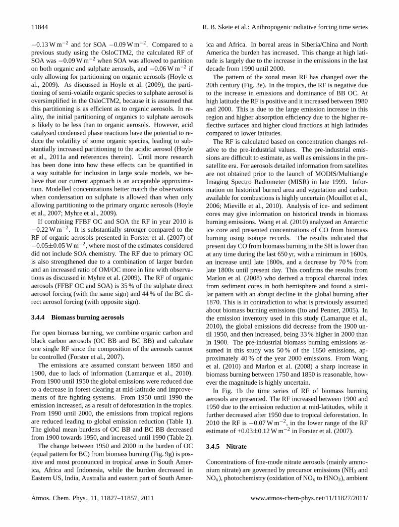
Figure 3: Zonal mean RF for selected years for tropospheric ozone (a), directaerosol effect of sulphate (b), FFBF BC (c), FFBF OC (d), SOA (e), BB aerosols(f), nitrate (g), total direct aerosol effect (h) and the cloud albedo effect (i).
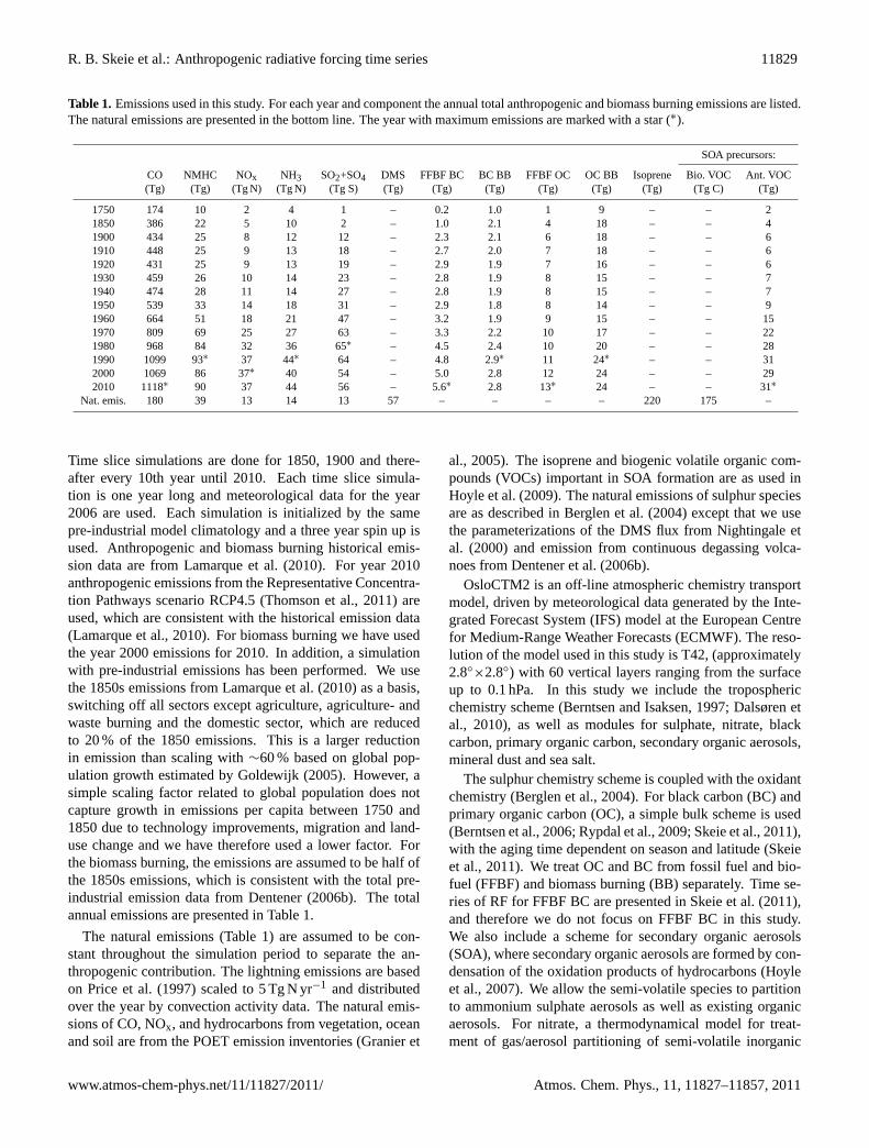
Fig. 3. Zonal mean RF for selected years for tropospheric ozone(a), direct aerosol effect of sulphate(b), FFBF BC(c), FFBF OC(d), SOA(e), BB aerosols(f), nitrate(g), total direct aerosol effect(h) and the cloud albedo effect(i).
high altitude at mid-latitudes in the NH due to convectivetransport from the boundary layer and emissions from avia-tion. At high altitudes, above the equator, there is a decreasein the NOx concentrations. This is in the same region as OHdecreased (Fig. 2e) due to increased loss through reactionwith CO and CH4 leading to increased HO2 concentration.The decrease in NOx in this region is compensated by an in-crease in other forms of reactive nitrogen, mainly HO2NO2,with small contribution from PAN and less contribution fromHNO3 (Fig. 2f).
Figure 3 shows the calculated zonal mean RF for selectedyears. Tropospheric O3 RF has a similar distribution for eachdecade, with a maximum at 20◦ N and a secondary maxi-mum at 20◦ S (Fig. 3a). The largest RF in the NH is foundin the Middle East, and in the Southern Hemisphere (SH)
the strongest RF is located downwind from biomass burningareas.
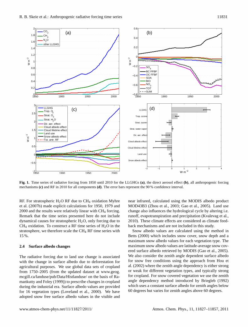
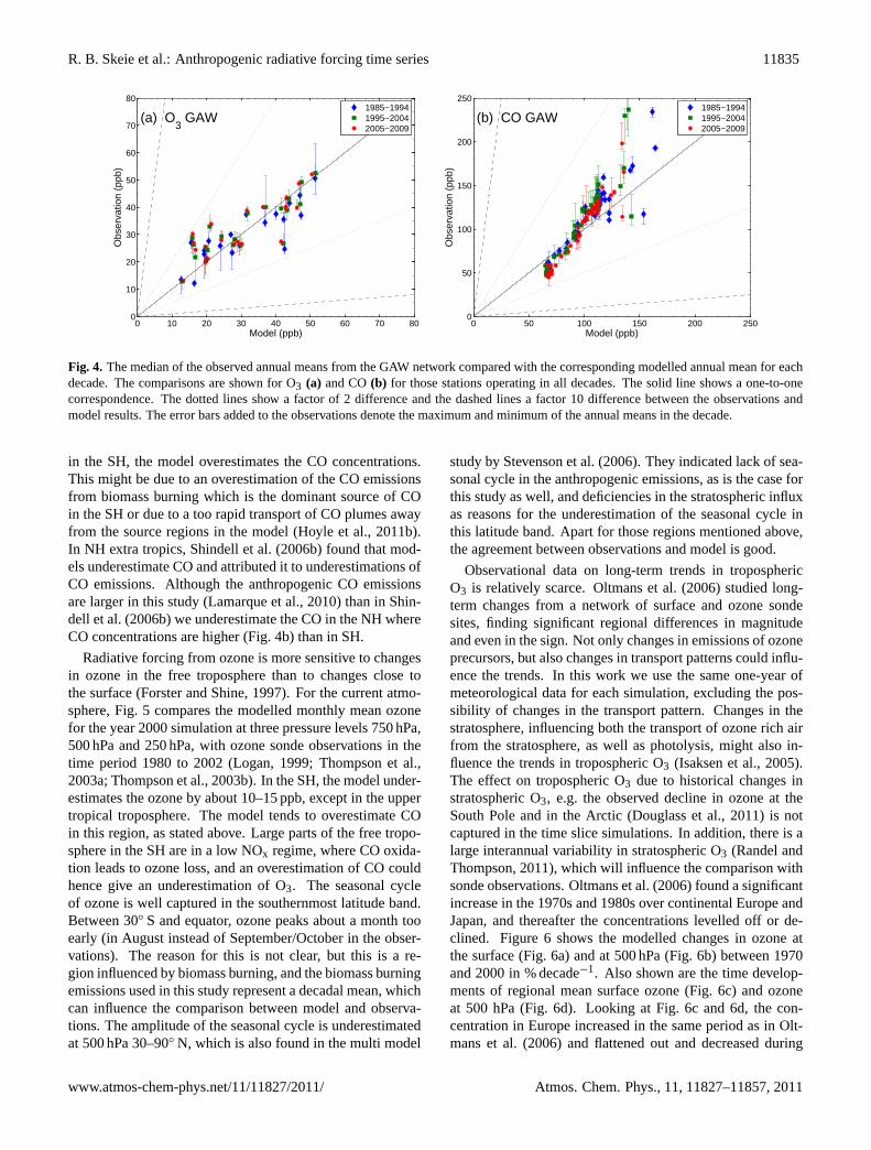
There are limited observations in space and time that canbe used to validate the modelled trend of tropospheric O3.During the last decades, surface ozone has been measuredat several sites around the world. Figure 4a compares themodelled and observed surface ozone from the Global At-mospheric Watch (GAW) network. The figure compares thedecadal median of the observed annual mean and the annualmean from the time slice simulations. The comparison isshown for those stations reporting observations in all threedecades. A good representation of ozone at remote stationsfor the last decades is found with a correlation coefficientof 0.7. In Fig. 4b, modelled and observed CO are plotted.For low observed values, which are located in remote areas
R. B. Skeie et al.: Anthropogenic radiative forcing time series 11835
0 10 20 30 40 50 60 70 800
10
20
30
40
50
60
70
80
Model (ppb)
Obs
erva
tion
(ppb
)
1985−19941995−20042005−2009
(a) O3 GAW
0 50 100 150 200 2500
50
100
150
200
250
Model (ppb)
Obs
erva
tion
(ppb
)
1985−19941995−20042005−2009
(b) CO GAW
Figure 4: The median of the observed annual means from the GAW networkcompared with the corresponding modelled annual mean for each decade. Thecomparisons are shown for O3 (a) and CO (b) for those stations operating inall decades. The solid line shows a one-to-one correspondence. The dotted linesshow a factor of 2 difference and the dashed lines a factor 10 difference betweenthe observations and model results. The error bars added to the observationsdenote the maximum and minimum of the annual means in the decade.
Fig. 4. The median of the observed annual means from the GAW network compared with the corresponding modelled annual mean for eachdecade. The comparisons are shown for O3 (a) and CO(b) for those stations operating in all decades. The solid line shows a one-to-onecorrespondence. The dotted lines show a factor of 2 difference and the dashed lines a factor 10 difference between the observations andmodel results. The error bars added to the observations denote the maximum and minimum of the annual means in the decade.
in the SH, the model overestimates the CO concentrations.This might be due to an overestimation of the CO emissionsfrom biomass burning which is the dominant source of COin the SH or due to a too rapid transport of CO plumes awayfrom the source regions in the model (Hoyle et al., 2011b).In NH extra tropics, Shindell et al. (2006b) found that mod-els underestimate CO and attributed it to underestimations ofCO emissions. Although the anthropogenic CO emissionsare larger in this study (Lamarque et al., 2010) than in Shin-dell et al. (2006b) we underestimate the CO in the NH whereCO concentrations are higher (Fig. 4b) than in SH.
Radiative forcing from ozone is more sensitive to changesin ozone in the free troposphere than to changes close tothe surface (Forster and Shine, 1997). For the current atmo-sphere, Fig. 5 compares the modelled monthly mean ozonefor the year 2000 simulation at three pressure levels 750 hPa,500 hPa and 250 hPa, with ozone sonde observations in thetime period 1980 to 2002 (Logan, 1999; Thompson et al.,2003a; Thompson et al., 2003b). In the SH, the model under-estimates the ozone by about 10–15 ppb, except in the uppertropical troposphere. The model tends to overestimate COin this region, as stated above. Large parts of the free tropo-sphere in the SH are in a low NOx regime, where CO oxida-tion leads to ozone loss, and an overestimation of CO couldhence give an underestimation of O3. The seasonal cycleof ozone is well captured in the southernmost latitude band.Between 30◦ S and equator, ozone peaks about a month tooearly (in August instead of September/October in the obser-vations). The reason for this is not clear, but this is a re-gion influenced by biomass burning, and the biomass burningemissions used in this study represent a decadal mean, whichcan influence the comparison between model and observa-tions. The amplitude of the seasonal cycle is underestimatedat 500 hPa 30–90◦ N, which is also found in the multi model
study by Stevenson et al. (2006). They indicated lack of sea-sonal cycle in the anthropogenic emissions, as is the case forthis study as well, and deficiencies in the stratospheric influxas reasons for the underestimation of the seasonal cycle inthis latitude band. Apart for those regions mentioned above,the agreement between observations and model is good.
Observational data on long-term trends in troposphericO3 is relatively scarce. Oltmans et al. (2006) studied long-term changes from a network of surface and ozone sondesites, finding significant regional differences in magnitudeand even in the sign. Not only changes in emissions of ozoneprecursors, but also changes in transport patterns could influ-ence the trends. In this work we use the same one-year ofmeteorological data for each simulation, excluding the pos-sibility of changes in the transport pattern. Changes in thestratosphere, influencing both the transport of ozone rich airfrom the stratosphere, as well as photolysis, might also in-fluence the trends in tropospheric O3 (Isaksen et al., 2005).The effect on tropospheric O3 due to historical changes instratospheric O3, e.g. the observed decline in ozone at theSouth Pole and in the Arctic (Douglass et al., 2011) is notcaptured in the time slice simulations. In addition, there is alarge interannual variability in stratospheric O3 (Randel andThompson, 2011), which will influence the comparison withsonde observations. Oltmans et al. (2006) found a significantincrease in the 1970s and 1980s over continental Europe andJapan, and thereafter the concentrations levelled off or de-clined. Figure 6 shows the modelled changes in ozone atthe surface (Fig. 6a) and at 500 hPa (Fig. 6b) between 1970and 2000 in % decade−1. Also shown are the time develop-ments of regional mean surface ozone (Fig. 6c) and ozoneat 500 hPa (Fig. 6d). Looking at Fig. 6c and 6d, the con-centration in Europe increased in the same period as in Olt-mans et al. (2006) and flattened out and decreased during
11836 R. B. Skeie et al.: Anthropogenic radiative forcing time series
Figure 5: Comparison of the annual cycle of ozone observations (black dots) andmonthly mean O3 for the year 2000 simulation (gray lines) at different latitudebands and at different pressure levels (750 hPa, 500 hPa and 250 hPa). O3 sondedata are from Logan (1999) and Thompson et al. (2003a, 2003b). The numberof sites is given in the top right corner of each plot. The figure is similar as inthe multi model study by Stevenson et al. (2006).
Fig. 5. Comparison of the annual cycle of ozone observations (black dots) and monthly mean O3 for the year 2000 simulation (gray lines) atdifferent latitude bands and at different pressure levels (750 hPa, 500 hPa and 250 hPa). O3 sonde data are from Logan (1999) and Thompsonet al. (2003a, b). The number of sites is given in the top right corner of each plot. The figure is similar as in the multi model study byStevenson et al. (2006).
the last decades. In the model, the ozone concentrations in-crease more on the western coast than on the eastern coastof North America due to influence of emission increase inEastern Asia in the recent decades (Fig. 6). A rapid increasein observed springtime tropospheric O3 is also observed atthe US Pacific coast in the recent years (Parrish et al., 2004;Cooper et al., 2010) which is related to increased Asian emis-sions. Looking at Fig. 6b, the largest increase in ozone at500 hPa is in Middle East, South, South East and East Asiabetween 1970s and year 2000. However, no observed long-term trends in tropospheric O3 from these regions exist.
Lelieveld et al. (2004) published trends in O3 over the At-lantic from ship-borne measurements from 1977 to 2002. Nosignificant increase in O3 at high latitudes was found, whilelarger trends in ozone are found at lower latitudes and inthe SH. In the OsloCTM2, the largest trends in the Atlanticare found outside the North African coast with 0.15 ppb yr−1
between 1980 and 2000, a spatial pattern consistent withLelieveld et al. (2004). However, the observed increase is0.5 ppb yr−1 between 20–40◦ N a factor of∼3 larger thanthe modelled trend. It should be noted that the observationsprior to 1995 are sparse in Lelieveld et al. (2004) and thetrend may be influenced by the seasonal O3 trend.
One of the longest records of measured O3 is from Ho-henpeissenberg, Germany (11.0◦ E, 47.8◦ N, 985 m) and goesback to 1970. The modelled annual surface ozone for thisstation is plotted together with 12 month running mean ofthe surface observations in Fig. 7a. In the 1970s and 1980s,the model tends to over predict the observations, while betteragreement is found for the last decade. At Arkona (13.4◦ E,54.7◦ N) in Northern Germany at the Baltic Sea, surface mea-surements of O3 started in the 1950s (German Meteorologi-cal Service of the German Democratic Republic). Also here,the ozone increase in the 1970s is not as sharp as observed(Fig. 6b), however the pre-1972 Arkona data might not beconsistent with the later period (Low et al., 1990) due tochanges in measurement instruments.
In Switzerland, in Arosa (9.7◦ E, 46.8◦ N, 1800 m) O3measurements were also made in the 1950s. The O3 concen-tration increased by a factor of 2.2 between 1950s and 1990(Staehelin et al., 1994). From our model results the annualmean concentrations increased by only 45 %, from 32 ppb in1950s to 46.5 ppb in 1990s.
Further back in time, from the 19th century, measurementsof tropospheric O3 based on Schonbein paper methods exist.High uncertainties due to calibration, humidity, and other
Western North America (135W−90W; 30N−60N)Eastern North America (90W−45W; 30N−60N)Europe (0E−45E; 35N−65N)Middle East (40E−55E;20N−35N)East Asia (100E−145E;30N−60N)Southern Africa (0E−45E;35S−0S)Southern America (90W−45W;30S−0S)Southern Asia (65E−100E;0N−30N)
(c)
1850 1870 1890 1910 1930 1950 1970 1990 201020
25
30
35
40
45
50
55
60
65
70
ppb
Western North America (135W−90W; 30N−60N)Eastern North America (90W−45W; 30N−60N)Europe (0E−45E; 35N−65N)Middle East (40E−55E;20N−35N)East Asia (100E−145E;30N−60N)Southern Africa (0E−45E;35S−0S)Southern America (90W−45W;30S−0S)Southern Asia (65E−100E;0N−30N)
(d)
Figure 6: Relative change from 1970 to 2000 (% decade−1) in surface O3 (a) andat approximately 500 hPa (b) and time evolution of regional mean O3 at thesurface (c) and approximately 500 hPa (d).
Fig. 6. Relative change from 1970 to 2000 (% decade−1) in surface O3 (a) and at approximately 500 hPa(b) and time evolution of regionalmean O3 at the surface(c) and approximately 500 hPa(d).
1940 1950 1960 1970 1980 1990 2000 20100
10
20
30
40
50
60
70
80
O3 p
pb
HohenpeissenbergOslo−CTM2 results (a)
1940 1950 1960 1970 1980 1990 2000 20100
20
40
60
80
100
120
O3 µ
g m
−3
ArkonaOslo−CTM2 results (b)
Figure 7: Time series of surface O3 at Hohenpeissenberg (a) and Arkona (b).Annual mean model values (black dots) and 12-month smoothed average for theobservations (solid line).
Fig. 7. Time series of surface O3 at Hohenpeissenberg(a) and Arkona(b). Annual mean model values (black dots) and 12-month smoothedaverage for the observations (solid line).
pollutants confounding the measurements make these mea-surements quantitatively unreliable (Pavelin et al., 1999). AtPic du Midi (0.15◦ E, 49.9◦ N) in France at 3000 m altitude,there exist observed ozone from 1874 to 1909 (Marenco etal., 1994). A stable concentration of 10 ppb was found until
1895 then concentration tends to increase. Combined withobserved surface O3 in the 1990s, this gives a five fold con-centration increase at this station. Marenco et al. (1994) sum-marized other measurement done in the 19th century giving apre-industrial O3 level of 10±3.5 ppb. However in our model
11838 R. B. Skeie et al.: Anthropogenic radiative forcing time series
results, as in a number of previous model simulations (e.g.Wang and Jacob, 1998; Berntsen et al., 2000; Lamarque etal., 2005; Shindell et al., 2006a; Lamarque et al., 2010) weare not able to simulate these low values in the 19th cen-tury. As seen in Fig. 6c, the surface ozone in the regionsconsidered ranged between 15 and 18 ppb in 1850. Mick-ley et al. (2001) showed that reducing the soil and lightningNOx emissions and increasing biogenic VOC emissions inthe model gives a better match of the 19th century observa-tions. If this is true, it still leaves open the question if the nat-ural emission changes are climate feedbacks, and GCM sim-ulations have shown increased lightning in a warmer climate(Price and Rind, 1994; Hauglustaine et al., 2005; Brasseur etal., 2006; Del Genio et al., 2007).
The uncertainty range in the tropospheric O3 radiativeforcing in Forster et al. (2007) was skewed ranging from0.25 to 0.65 W m−2 with a best estimate of 0.35 W m−2.This range took into account model results tuning the nat-ural emissions to reproduce the low ozone values reportedfrom the 19th century. Due to the large uncertainties in themeasurements from the 19th century and that we considerchanges in the natural emissions as a feedback on the cli-mate system, we exclude those results where natural emis-sions were tuned, presenting a symmetric uncertainty rangeof ±30 % in Fig. 1d, 0.44±0.13 W m−2. Our troposphericO3 RF estimate includes 0.03 W m−2 from changes in thestratosphere due to tropospheric O3 precursors. Søvde etal. (2011) calculated chemistry in the whole stratosphere us-ing the OsloCTM2 and found a stronger effect of 0.08 W m−2
in the stratosphere.
3.2.2 The oxidation capacity
The hydroxyl radical (OH) is the major oxidation compo-nent in the atmosphere and has therefore a great impact onthe concentrations of CH4 and the ozone precursors, therebyaffecting tropospheric O3. In our model, the historical CH4concentrations are however based on observed historical CH4concentration.
Figure 2e shows the difference in the zonal annual meanconcentration of OH between 1950 and 2000. There are twocompeting effects, an increase in NOx gives an increase inthe OH concentration, and increases in CH4 and CO whichreduce the OH concentration. Since the concentration changeof NOx is greatest close to the surface in industrialized re-gions (Fig. 2c) while CO (Fig. 2d) and CH4 concentrationchanges are more evenly distributed in the atmosphere, theincrease in OH is seen close to the surface, while in the freetroposphere the OH is reduced (Fig. 2e).
In our simulations, the global average of OH concentra-tion decreased by 15 % from 1850 until year 2000 (Fig. 8).The largest rate of change is found between 1950 and 1960with a decrease of 3 % decade−1. The concentration lev-elled off at the end of the simulation period, 1990–2010,at 1.1×10⁶ molecules cm−3. Pozzoli et al. (2011) calculated
1850 1900 1950 20000.8
0.9
1
1.1
1.2
1.3
1.4
1.5
[OH
] 106 m
olec
/cm
3
Oslo−CTM2 resultsBousquet et al. 2006
Figure 8: Modelled annual mean global OH concentration (black dots) and de-rived OH concentrations (solid line) with uncertainties (dotted lines) from Bous-quet et al. (2006).
Fig. 8. Modelled annual mean global OH concentration (black dots)and derived OH concentrations (solid line) with uncertainties (dot-ted lines) from Bousquet et al. (2006).
changes in global OH concentration from 1980 to 2005 usingthe aerosol-chemistry-climate model ECHAM5-HAMMOZ.They found an increasing trend due to anthropogenic emis-sions of 0.25 % yr−1 which is greater than the relatively sta-ble OH concentration in our study over this period (Fig. 8).Pozzoli et al. (2011) found that the anthropogenic trend wasoffset by a decreasing OH trend due to natural variability inmeteorology (lightning, humidity and temperature) and nat-ural emissions including biomass burning emissions empha-sising the role of other factors than anthropogenic emissionson the OH concentration. The global mean OH concen-tration can be estimated based on observations of gases re-moved from the atmosphere by reactions with OH. Bousquetet al. (2005) looked at the OH variability in the 1980s and1990s using methyl chloroform observations. The inferredOH concentration from Bousquet et al. (2005) is added inFig. 8. There is a large interannual variability in the inferredOH concentrations, but a downward trend is seen. The trendis larger than what we find in the model results. Recently,Montzka et al. (2011a), found that the OH concentration hasbeen rather stable over the last decade, which is consistentwith our model results (Fig. 8) and Pozzoli et al. (2011).
3.3 Stratospheric ozone and water vapour
In Fig. 1c the radiative forcing time series of stratosphericO3 is shown. The RF starts decreasing in the 1950s whenconcentrations of ozone depleting components in the strato-sphere increases. The minimum RF is reached at the endof the 1990s, due to a reduction in the EESC at the endof the 20th century. The stratospheric O3 RF in 2010 is−0.23 W m−2 (Fig. 1d).
Our estimate accounts for changes in ozone due to ozonedepleting components, occurring both in the stratosphere
R. B. Skeie et al.: Anthropogenic radiative forcing time series 11839
and in the troposphere. The RF presented in IPCC 2007of −0.05±0.1 W m−2 (Forster et al., 2007) is due to ozonechanges in the stratosphere, and more recently Forsteret al. (2011) presented a 1970s to 2004 radiative forc-ing estimate of +0.03 W m−2 based on observations and−0.03±0.2 W m−2 based on chemistry climate models simu-lations, but stated that the estimates are not entirely of anthro-pogenic origin. Cionni et al. (2011) found a stratospheric O3RF of −0.08 W m−2, based on observations of stratosphericO3 from satellites and sonde data. The RF of stratospheric O3changes given in Søvde et al. (2011) due to both chlorine andbromine and tropospheric O3 precursors was−0.12 W m−2,within the ranges above but in the stronger range of previousstudies. Radiative forcing estimates of ozone changes in thetroposphere due to chlorine and bromine have not previouslybeen published, but in Gauss et al. (2006), significant effectson tropospheric O3 RF due to chlorine and bromine wereseen. A subjective choice of an uncertainty bar of±70 %is added in Fig. 1d for stratospheric O3 RF giving a rangeof −0.07 to−0.39 W m−2. Not included in this estimate isthe effect of N2O on stratospheric O3, which was not con-sidered in Søvde et al. (2011). A small RF of this effect of−0.01 W m−2 was given in Forster et al. (2007) in Table 2.13.
The RF of stratospheric water vapour increases through-out the period, but flattens out over the last decades (Fig. 1c),as seen for the RF of CH4 as well. The RF is estimatedby scaling the RF estimate for year 2005 in Forster etal. (2007) and the same relative uncertainties as in Forsteret al. (2007) (±71 %) is adopted. This gives a RF in 2010of 0.073±0.052 W m−2 (Fig. 1d).The best estimate of strato-spheric H2O RF is 2.6 % of the RF of LLGHG in 2010.
3.4 Aerosols
In this section the changes in the aerosol concentrations andthe direct aerosol effect for each aerosol component is firstpresented. In Sect. 3.4.6, the time series of the total directaerosol effect and in Sect. 3.4.7 the indirect aerosol effects,both the cloud albedo effect and the cloud lifetime effect,are presented. The resulting RF time series are plotted inFig. 1. The direct aerosol effect separated for each aerosolcomponent is plotted in Fig. 1b, and we see that the two mainaerosol components causing RF are sulphate and BC.
3.4.1 Sulphate
The total anthropogenic SO2 emission reached its maximumof 65 Tg S year−1 in the 1980s (Table 1). The regional dis-tribution of the emissions has changed over the 20th cen-tury, with a southward shift in the SO2 emissions in the lastdecades. At lower latitudes, the oxidation capacity of the at-mosphere is higher (due to higher OH concentrations) andthe emissions of oxidants precursors have also shifted south-wards leading to a larger fraction of SO2 being oxidized tosulphate.
A summary of the global burden increase since 1750 isgiven in Table 2. As much as 36 % of the total increase insulphate burden occurred before 1950, mainly in early in-dustrial areas in North America and Europe. Figure 9 showsthe change in the burden and zonal mean concentrations be-tween 1950 and 2000 for several aerosol components, as wellas changes in regional burdens since 1850. The southwardshift in the burden of SO4 is seen in Fig. 9a where the burdenis reduced over Europe, North Atlantic and Eurasian Arctic,while the burden increased in the Middle East, South Asiaand East Asia. The zonal mean concentration of sulphate in-creases south of 45◦ N throughout the troposphere while itmainly decreases in the north (Fig. 9b).
There was a particularly sharp increase in the sulphateburden over Europe from 1950 to 1970 (52 % decade−1)(Fig. 9c). After 1980 the burden over Europe has droppedand in year 2000 the burden was back to the 1950 level. Foreastern North America, the burden has decreased since the1970s. In the Middle East and East Asia, the burden in-creased gradually since the 1950s, while in South Asia theburden increased more rapidly.
The increase in sulphate burden in 2000 since 1850 was0.44 Tg S (2.6 mg (SO4) m−2), compared to the increase inburden of 0.36 Tg S (2.1 mg (SO4) m−2) in Lamarque etal. (2010) who used the same emission inventory. In the Ae-roCom study (Schulz et al., 2006), the burden increase sincepre-industrial times was 2.12 mg (SO4) m−2 (standard devi-ation of 0.82 mg (SO4) m−2). Summarizing previous stud-ies, Schulz et al. (2006) found a larger increase in sulphateburden of 2.70 mg (SO4) m−2 (standard deviation of 1.09 mg(SO4) m−2), which is in good agreement with our increase inburden in 2000 relative to 1750 of 2.79 mg (SO4) m−2.
The modelled maximum of the sulphate burden in ourstudy occurred in the 1980s and 1990s, consistent with thestudy by Boucher and Pham (2002). Since the 1980s, the to-tal (anthropogenic) emission of sulphur is reduced by∼15 %while the anthropogenic burden of SO4 is only reduced by∼4 %. The southward shift in the emissions, to regionswith higher oxidation capacity enhances the SO4 produc-tion efficiency, and the lifetime of SO4 remained fairly con-stant (±4 %). As also was found in Berglen et al. (2007),the reduction of emissions of SO2 in Europe between 1985and 1996 gave an increase in the efficiency of oxidationto sulphate. Similar results were also found by Pozzoli etal. (2011) for the period 1980 to 2005 with an almost un-changed global mean burden between a simulation with vary-ing and fixed anthropogenic emissions.
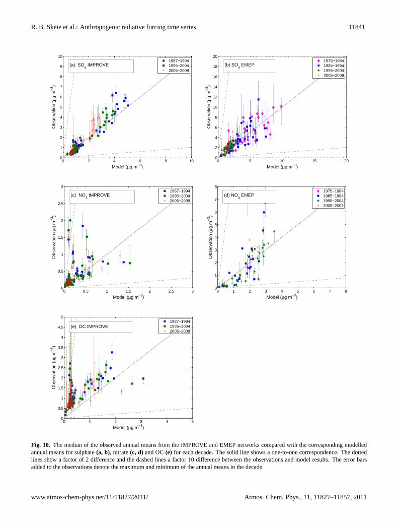
Figure 10 compares observations and correspondingmodel results for several aerosol types. The figure showsdecadal median of annual mean concentrations compared tothe corresponding model results. Only the sites that havemeasurements in the 1980s, 1990s and 2000s are included.Sulphate is compared with observations from the EMEP net-work in Europe (Fig. 10a) and with observations from theIMPROVE network in the United States (Fig. 10b). For
Western North America (135W−90W; 30N−60N)Eastern North America (90W−45W; 30N−60N)Europe (0E−45E; 35N−65N)Middle East (40E−55E;20N−35N)East Asia (100E−145E;30N−60N)Southern Africa (0E−45E;35S−0S)Southern America (90W−45W;30S−0S)Southern Asia (65E−100E;0N−30N)
Western North America (135W−90W; 30N−60N)Eastern North America (90W−45W; 30N−60N)Europe (0E−45E; 35N−65N)Middle East (40E−55E;20N−35N)East Asia (100E−145E;30N−60N)Southern Africa (0E−45E;35S−0S)Southern America (90W−45W;30S−0S)Southern Asia (65E−100E;0N−30N)
Western North America (135W−90W; 30N−60N)Eastern North America (90W−45W; 30N−60N)Europe (0E−45E; 35N−65N)Middle East (40E−55E;20N−35N)East Asia (100E−145E;30N−60N)Southern Africa (0E−45E;35S−0S)Southern America (90W−45W;30S−0S)Southern Asia (65E−100E;0N−30N)
Western North America (135W−90W; 30N−60N)Eastern North America (90W−45W; 30N−60N)Europe (0E−45E; 35N−65N)Middle East (40E−55E;20N−35N)East Asia (100E−145E;30N−60N)Southern Africa (0E−45E;35S−0S)Southern America (90W−45W;30S−0S)Southern Asia (65E−100E;0N−30N)
Western North America (135W−90W; 30N−60N)Eastern North America (90W−45W; 30N−60N)Europe (0E−45E; 35N−65N)Middle East (40E−55E;20N−35N)East Asia (100E−145E;30N−60N)Southern Africa (0E−45E;35S−0S)Southern America (90W−45W;30S−0S)Southern Asia (65E−100E;0N−30N)
(o)
Figure 9: The 2000-1950 difference in annual mean column load (left column) andannual zonal mean concentration (middle column). The development in regionalburden relative to 1850 is shown in the right column. The aerosols included aresulphate, FFBF OC, BB OC, SOA and fine mode nitrate.
Fig. 9. The 2000–1950 difference in annual mean column load (left column) and annual zonal mean concentration (middle column). Thedevelopment in regional burden relative to 1850 is shown in the right column. The aerosols included are sulphate, FFBF OC, BB OC, SOAand fine mode nitrate.
R. B. Skeie et al.: Anthropogenic radiative forcing time series 11841
0 2 4 6 8 100
1
2
3
4
5
6
7
8
9
10
Model (µg m−3)
Obs
erva
tion
(µg
m−
3 )
1987−19941995−20042005−2009
(a) SO4 IMPROVE
0 5 10 15 200
2
4
6
8
10
12
14
16
18
20
Model (µg m−3)
Obs
erva
tion
(µg
m−
3 )
1975−19841985−19941995−20042005−2009
(b) SO4 EMEP
0 0.5 1 1.5 2 2.5 30
0.5
1
1.5
2
2.5
3
Model (µg m−3)
Obs
erva
tion
(µg
m−
3 )
1987−19941995−20042005−2009
(c) NO3 IMPROVE
0 1 2 3 4 5 6 7 80
1
2
3
4
5
6
7
8
Model (µg m−3)
Obs
erva
tion
(µg
m−
3 )
1975−19841985−19941995−20042005−2009
(d) NO3 EMEP
0 1 2 3 4 50
0.5
1
1.5
2
2.5
3
3.5
4
4.5
5
Model (µg m−3)
Obs
erva
tion
(µg
m−
3 )
1987−19941995−20042005−2009
(e) OC IMPROVE
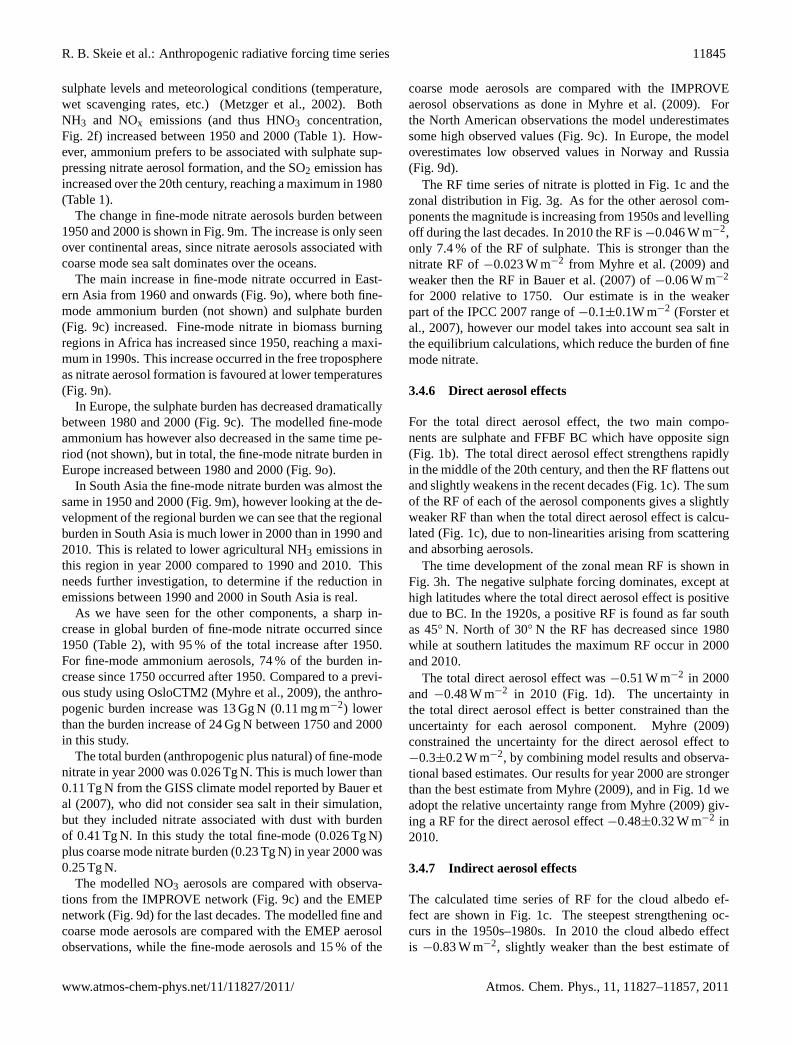
Figure 10: The median of the observed annual means from the IMPROVE andEMEP networks compared with the corresponding modelled annual means forsulphate (a,b), nitrate (c,d) and OC (e) for each decade. The solid line shows aone-to-one correspondence. The dotted lines show a factor of 2 difference and thedashed lines a factor 10 difference between the observations and model results.The error bars added to the observations denote the maximum and minimum ofthe annual means in the decade.
Fig. 10. The median of the observed annual means from the IMPROVE and EMEP networks compared with the corresponding modelledannual means for sulphate(a, b), nitrate(c, d) and OC(e) for each decade. The solid line shows a one-to-one correspondence. The dottedlines show a factor of 2 difference and the dashed lines a factor 10 difference between the observations and model results. The error barsadded to the observations denote the maximum and minimum of the annual means in the decade.
11842 R. B. Skeie et al.: Anthropogenic radiative forcing time series
1850 1870 1890 1910 1930 1950 1970 1990 20100
0.5
1
1.5
2
2.5
Rel
ativ
e de
posi
tion
ACT2 Ice CoreACT2 modelled
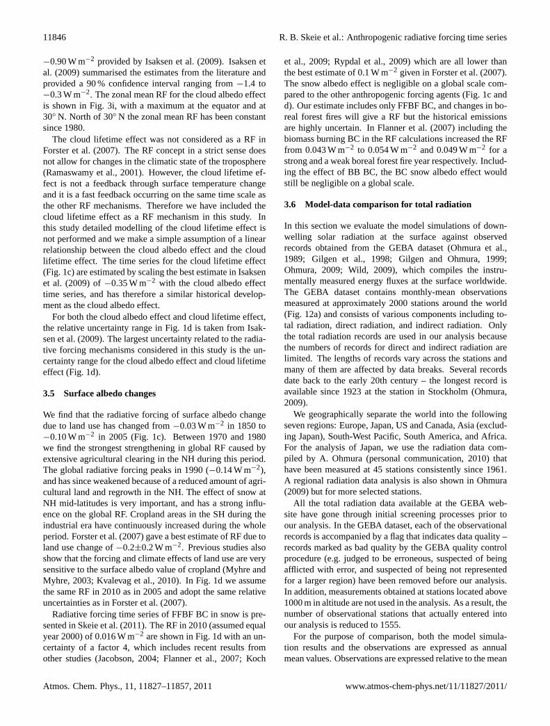
Figure 11: Modelled relative deposition of sulphur (red dots) and relative depo-sition of sulphur from ACT2 ice core (solid line) in Greenland (McConnell andEdwards et al. 2008). The annual depositions are plotted relative to the meandeposition between 1900 and 2000.
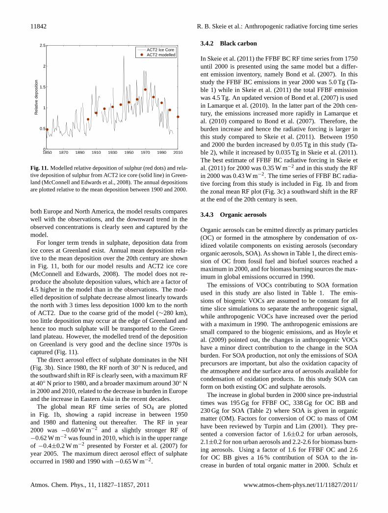
Fig. 11.Modelled relative deposition of sulphur (red dots) and rela-tive deposition of sulphur from ACT2 ice core (solid line) in Green-land (McConnell and Edwards et al., 2008). The annual depositionsare plotted relative to the mean deposition between 1900 and 2000.
both Europe and North America, the model results compareswell with the observations, and the downward trend in theobserved concentrations is clearly seen and captured by themodel.
For longer term trends in sulphate, deposition data fromice cores at Greenland exist. Annual mean deposition rela-tive to the mean deposition over the 20th century are shownin Fig. 11, both for our model results and ACT2 ice core(McConnell and Edwards, 2008). The model does not re-produce the absolute deposition values, which are a factor of4.5 higher in the model than in the observations. The mod-elled deposition of sulphate decrease almost linearly towardsthe north with 3 times less deposition 1000 km to the northof ACT2. Due to the coarse grid of the model (∼280 km),too little deposition may occur at the edge of Greenland andhence too much sulphate will be transported to the Green-land plateau. However, the modelled trend of the depositionon Greenland is very good and the decline since 1970s iscaptured (Fig. 11).
The direct aerosol effect of sulphate dominates in the NH(Fig. 3b). Since 1980, the RF north of 30◦ N is reduced, andthe southward shift in RF is clearly seen, with a maximum RFat 40◦ N prior to 1980, and a broader maximum around 30◦ Nin 2000 and 2010, related to the decrease in burden in Europeand the increase in Eastern Asia in the recent decades.
The global mean RF time series of SO4 are plottedin Fig. 1b, showing a rapid increase in between 1950and 1980 and flattening out thereafter. The RF in year2000 was −0.60 W m−2 and a slightly stronger RF of−0.62 W m−2 was found in 2010, which is in the upper rangeof −0.4±0.2 W m−2 presented by Forster et al. (2007) foryear 2005. The maximum direct aerosol effect of sulphateoccurred in 1980 and 1990 with−0.65 W m−2.
3.4.2 Black carbon
In Skeie et al. (2011) the FFBF BC RF time series from 1750until 2000 is presented using the same model but a differ-ent emission inventory, namely Bond et al. (2007). In thisstudy the FFBF BC emissions in year 2000 was 5.0 Tg (Ta-ble 1) while in Skeie et al. (2011) the total FFBF emissionwas 4.5 Tg. An updated version of Bond et al. (2007) is usedin Lamarque et al. (2010). In the latter part of the 20th cen-tury, the emissions increased more rapidly in Lamarque etal. (2010) compared to Bond et al. (2007). Therefore, theburden increase and hence the radiative forcing is larger inthis study compared to Skeie et al. (2011). Between 1950and 2000 the burden increased by 0.05 Tg in this study (Ta-ble 2), while it increased by 0.035 Tg in Skeie et al. (2011).The best estimate of FFBF BC radiative forcing in Skeie etal. (2011) for 2000 was 0.35 W m−2 and in this study the RFin 2000 was 0.43 W m−2. The time series of FFBF BC radia-tive forcing from this study is included in Fig. 1b and fromthe zonal mean RF plot (Fig. 3c) a southward shift in the RFat the end of the 20th century is seen.
3.4.3 Organic aerosols
Organic aerosols can be emitted directly as primary particles(OC) or formed in the atmosphere by condensation of ox-idized volatile components on existing aerosols (secondaryorganic aerosols, SOA). As shown in Table 1, the direct emis-sion of OC from fossil fuel and biofuel sources reached amaximum in 2000, and for biomass burning sources the max-imum in global emissions occurred in 1990.
The emissions of VOCs contributing to SOA formationused in this study are also listed in Table 1. The emis-sions of biogenic VOCs are assumed to be constant for alltime slice simulations to separate the anthropogenic signal,while anthropogenic VOCs have increased over the periodwith a maximum in 1990. The anthropogenic emissions aresmall compared to the biogenic emissions, and as Hoyle etal. (2009) pointed out, the changes in anthropogenic VOCshave a minor direct contribution to the change in the SOAburden. For SOA production, not only the emissions of SOAprecursors are important, but also the oxidation capacity ofthe atmosphere and the surface area of aerosols available forcondensation of oxidation products. In this study SOA canform on both existing OC and sulphate aerosols.
The increase in global burden in 2000 since pre-industrialtimes was 195 Gg for FFBF OC, 338 Gg for OC BB and230 Gg for SOA (Table 2) where SOA is given in organicmatter (OM). Factors for conversion of OC to mass of OMhave been reviewed by Turpin and Lim (2001). They pre-sented a conversion factor of 1.6±0.2 for urban aerosols,2.1±0.2 for non urban aerosols and 2.2-2.6 for biomass burn-ing aerosols. Using a factor of 1.6 for FFBF OC and 2.6for OC BB gives a 16 % contribution of SOA to the in-crease in burden of total organic matter in 2000. Schulz et
R. B. Skeie et al.: Anthropogenic radiative forcing time series 11843
al. (2006) reported an increase in particulate organic matterof 1.32 mg m−2 (standard deviation 0.32 mg m−2) from theAeroCom simulations and 2.40 mg m−2 (standard deviationof 0.39 mg m−2) from other published estimates. Using thesame factors as above we find an increase in burden of or-ganic matter in year 2000 of 2.79 mg m−2 (1.42 Tg) includ-ing SOA and 2.34 mg m−2 (1.19 Tg) excluding SOA, a largerincrease than in the AeroCom simulations but in agreementwith other previous published studies summarized in Schulzet al. (2006).
In Hoyle et al. (2009), the burden increase of SOA since1750 was 260 Gg when partitioning on sulphate aerosols wasallowed, larger than in this study (Table 2), which can be ex-plained by differeces in loading of sulphate and OC. Otherstudies calculating the change in SOA burden from pre-industrial times until present are Chung and Seinfeld (2002)with 130 Gg increase, Liao and Seinfeld (2005) with 100 Ggincrease and Tsigaridis et al. (2006) with 160 Gg increase.The increases in SOA burden from these models are lessthan what is calculated using OsloCTM2, although the rel-ative change in Chung and Seinfeld (2002) was greater. Thedifferences among the models, mainly related to the amountof mass available for partitioning, meteorological data, re-moval schemes, and biogenic VOC, are discussed in detail inHoyle et al. (2009).
The time development of global mean burden over the20th century differs for FFBF OC, OC BB and SOA. ForFFBF OC, the global mean burden increased almost linearlythroughout the century, while for OC BB, the burden washigher in the early 20th century and decreased towards 1950before increasing again until 1990 following the global emis-sions (Table 1). Between 1850 and 1950 the SOA burden in-creased almost linearly by 1 % decade−1 and after 1950 theburden increased rapidly with 36 % decade−1 until 1990 andbeing stable thereafter (Table 2).
Looking at the geographical distribution of the burdenchange, the burden of FFBF OC is reduced over a greaterarea in North America and Europe since 1950 (Fig. 9d), andthe FFBF OC burden is shifted southwards as clearly seen inthe zonal mean concentration change plot (Fig. 9e). Biomassburning OC burden has increased in South America, Africaand Indonesia since 1950 (Fig. 9g).
For SOA (Fig. 9m), a slight reduction in burden is foundover the north eastern coast of the US and in Northern Europebetween 1950 and 2000, related to the decrease in burdenof SO4 (Fig. 9a) and OC (Fig. 9d) in these regions. An in-crease in the SOA burden is found in South America, Africa,South-, Southeast- and East Asia (Fig. 9m), where the bur-dens of OC and SO4 have also increased. For the zonalmean, the concentration of SOA increased between 1950 and2000 (Fig. 9k) for the whole domain. Two maxima are foundclose to the surface, at the equator related to biomass burn-ing, and at 20◦ N related to fossil fuel aerosols. The increasein SOA stretches to a higher altitude than that of FFBF OCand OC BB, due to the secondary character of SOA and a
larger fraction of the oxidised organic components shiftingto the aerosol phase at cold temperatures.
Looking at the regional development of the organicaerosols, the FFBF OC burden decreased in Northern Amer-ica since the 1920s (Fig. 9f). In Europe, the burden increaseduntil 1940 and decreased rapidly between 1960 and 2000.The most rapid increase was in South Asia, after 1950, butthe regional burden also increased in East Asia, the MiddleEast and South Africa in the latter part of the 20th century.For SOA, the burden increased in Europe until 1980 (Fig. 9l).For the other regions, the burden change between 1900 and1950 was small, possible due to decreasing OC BB and in-creasing sulphate and FFBF OC burden. In Southern Amer-ica, the burden increased rapidly from 1950 to 1960 and con-tinued to increase until 1990. This is related to a large in-crease in the OC BB in this region (Fig. 9i).
How well are the organic aerosols modelled? Modelledconcentrations from the OsloCTM2 for the present day sit-uation are compared with surface observations in Myhre etal. (2009) and Hoyle et al. (2007). The OsloCTM2 un-derestimates organic aerosols at most of the stations, evenwhen all semi-volatile species are partitioned to the aerosolphase. Hoyle et al. (2007) suggested too low primary organicaerosols concentrations as one possible reason for the under-estimation, as well as sub-grid scale concentration gradients.
Long-term time series of OC measurements are only avail-able from the IMPROVE network. In Fig. 10e the observedOC concentrations are compared with modelled OC concen-trations assuming SOA concentration divided by the factorof 1.6 gives the carbon content. We see that the model tendsto under predict and grossly underestimate at several siteswhere the modelled concentrations of OC are very low. Thebest agreement is found for stations in eastern US, while theworst agreement is found for stations in the north westernUS. The underestimation is larger than in Myhre et al. (2009)and Hoyle et al. (2007) where modelled and observed con-centrations corresponding to the same year was compared.One reason for the underestimation in this study may there-fore be that we compare model results and observations fordifferent years. The meteorological situation influences theobserved concentrations, and biomass burning emissions arehighly variable. The OC burden in Hoyle et al. (2007) ishigher due to larger emissions and the use of a longer agingtime for conversion of OC from hydrophobic to hydrophilicaerosols.
In this section we focus on the radiative forcing of FFBFOC and SOA. Radiative forcing time series of biomass burn-ing aerosols will be presented in Sect. 3.4.4. As we saw forFFBF BC, the RF of FFBF OC is shifted southwards in thelatter part of the 20th century (Fig. 3d). For SOA there area broad maximum in RF between 10◦ S and 20◦ N in 2000(Fig. 3e), related to RF in South America, Africa and EasternAsia.
The RF time series of FFBF OC and SOA is plotted inFig. 1b. The calculated RF in 2010 for FFBF OC was
11844 R. B. Skeie et al.: Anthropogenic radiative forcing time series
−0.13 W m−2 and for SOA−0.09 W m−2. Compared to aprevious study using the OsloCTM2, the calculated RF ofSOA was−0.09 W m−2 when SOA was allowed to partitionon both organic and sulphate aerosols, and−0.06 W m−2 ifonly allowing for partitioning on organic aerosols (Hoyle etal., 2009). As discussed in Hoyle et al. (2009), the parti-tioning of semi-volatile organic species to sulphate aerosol isoversimplified in the OsloCTM2, because it is assumed thatthis partitioning is as efficient as to organic aerosols. In re-ality, the initial partitioning of organics to sulphate aerosolsis likely to be less than to organic aerosols. However, acidcatalysed condensed phase reactions have the potential to re-duce the volatility of some organic species, leading to sub-stantially increased partitioning to the acidic aerosol (Hoyleet al., 2011a and references therein). Until more researchhas been done into how these effects can be quantified ina way suitable for inclusion in large scale models, we be-lieve that our current approach is an acceptable approxima-tion. Modelled concentrations better match the observationswhen condensation on sulphate is allowed than when onlyallowing partitioning to the primary organic aerosols (Hoyleet al., 2007; Myhre et al., 2009).
If combining FFBF OC and SOA the RF in year 2010 is−0.22 W m−2. It is substantially stronger compared to theRF of organic aerosols presented in Forster et al. (2007) of−0.05±0.05 W m−2, where most of the estimates considereddid not include SOA chemistry. The RF due to primary OCis also strengthened due to a combination of larger burdenand an increased ratio of OM/OC more in line with observa-tions as discussed in Myhre et al. (2009). The RF of organicaerosols (FFBF OC and SOA) is 35 % of the sulphate directaerosol forcing (with the same sign) and 44 % of the BC di-rect aerosol forcing (with opposite sign).
3.4.4 Biomass burning aerosols
For open biomass burning, we combine organic carbon andblack carbon aerosols (OC BB and BC BB) and calculateone single RF since the composition of the aerosols cannotbe controlled (Forster et al., 2007).
The emissions are assumed constant between 1850 and1900, due to lack of information (Lamarque et al., 2010).From 1900 until 1950 the global emissions were reduced dueto a decrease in forest clearing at mid-latitude and improve-ments of fire fighting systems. From 1950 until 1990 theemission increased, as a result of deforestation in the tropics.From 1990 until 2000, the emissions from tropical regionsare reduced leading to global emission reduction (Table 1).The global mean burdens of OC BB and BC BB decreasedfrom 1900 towards 1950, and increased until 1990 (Table 2).
The change between 1950 and 2000 in the burden of OC(equal pattern for BC) from biomass burning (Fig. 9g) is pos-itive and most pronounced in tropical areas in South Amer-ica, Africa and Indonesia, while the burden decreased inEastern US, India, Australia and eastern part of South Amer-
ica and Africa. In boreal areas in Siberia/China and NorthAmerica the burden has increased. This change at high lati-tude is largely due to the increase in the emissions in the lastdecade from 1990 until 2000.
The pattern of the zonal mean RF has changed over the20th century (Fig. 3e). In the tropics, the RF is negative dueto the increase in emissions and dominance of BB OC. Athigh latitude the RF is positive and it increased between 1980and 2000. This is due to the large emission increase in thisregion and higher absorption efficiency due to the higher re-flective surfaces and higher cloud fractions at high latitudescompared to lower latitudes.
The RF is calculated based on concentration changes rel-ative to the pre-industrial values. The pre-industrial emis-sions are difficult to estimate, as well as emissions in the pre-satellite era. For aerosols detailed information from satellitesare not obtained prior to the launch of MODIS/MultiangleImaging Spectro Radiometer (MISR) in late 1999. Infor-mation on historical burned area and vegetation and carbonavailable for combustions is highly uncertain (Mouillot et al.,2006; Mieville et al., 2010). Analysis of ice- and sedimentcores may give information on historical trends in biomassburning emissions. Wang et al. (2010) analyzed an Antarcticice core and presented concentrations of CO from biomassburning using isotope records. The results indicated thatpresent day CO from biomass burning in the SH is lower thanat any time during the last 650 yr, with a minimum in 1600s,an increase until late 1800s, and a decrease by 70 % fromlate 1800s until present day. This confirms the results fromMarlon et al. (2008) who derived a tropical charcoal indexfrom sediment cores in both hemisphere and found a simi-lar pattern with an abrupt decline in the global burning after1870. This is in contradiction to what is previously assumedabout biomass burning emissions (Ito and Penner, 2005). Inthe emission inventory used in this study (Lamarque et al.,2010), the global emissions did decrease from the 1900 un-til 1950, and then increased, being 33 % higher in 2000 thanin 1900. The pre-industrial biomass burning emissions as-sumed in this study was 50 % of the 1850 emissions, ap-proximately 40 % of the year 2000 emissions. From Wanget al. (2010) and Marlon et al. (2008) a sharp increase inbiomass burning between 1750 and 1850 is reasonable, how-ever the magnitude is highly uncertain.
In Fig. 1b the time series of RF of biomass burningaerosols are presented. The RF increased between 1900 and1950 due to the emission reduction at mid-latitudes, while itfurther decreased after 1950 due to tropical deforestation. In2010 the RF is−0.07 W m−2, in the lower range of the RFestimate of +0.03±0.12 W m−2 in Forster et al. (2007).
3.4.5 Nitrate
Concentrations of fine-mode nitrate aerosols (mainly ammo-nium nitrate) are governed by precursor emissions (NH3 andNOx), photochemistry (oxidation of NOx to HNO3), ambient
R. B. Skeie et al.: Anthropogenic radiative forcing time series 11845
sulphate levels and meteorological conditions (temperature,wet scavenging rates, etc.) (Metzger et al., 2002). BothNH3 and NOx emissions (and thus HNO3 concentration,Fig. 2f) increased between 1950 and 2000 (Table 1). How-ever, ammonium prefers to be associated with sulphate sup-pressing nitrate aerosol formation, and the SO2 emission hasincreased over the 20th century, reaching a maximum in 1980(Table 1).
The change in fine-mode nitrate aerosols burden between1950 and 2000 is shown in Fig. 9m. The increase is only seenover continental areas, since nitrate aerosols associated withcoarse mode sea salt dominates over the oceans.
The main increase in fine-mode nitrate occurred in East-ern Asia from 1960 and onwards (Fig. 9o), where both fine-mode ammonium burden (not shown) and sulphate burden(Fig. 9c) increased. Fine-mode nitrate in biomass burningregions in Africa has increased since 1950, reaching a maxi-mum in 1990s. This increase occurred in the free troposphereas nitrate aerosol formation is favoured at lower temperatures(Fig. 9n).
In Europe, the sulphate burden has decreased dramaticallybetween 1980 and 2000 (Fig. 9c). The modelled fine-modeammonium has however also decreased in the same time pe-riod (not shown), but in total, the fine-mode nitrate burden inEurope increased between 1980 and 2000 (Fig. 9o).
In South Asia the fine-mode nitrate burden was almost thesame in 1950 and 2000 (Fig. 9m), however looking at the de-velopment of the regional burden we can see that the regionalburden in South Asia is much lower in 2000 than in 1990 and2010. This is related to lower agricultural NH3 emissions inthis region in year 2000 compared to 1990 and 2010. Thisneeds further investigation, to determine if the reduction inemissions between 1990 and 2000 in South Asia is real.
As we have seen for the other components, a sharp in-crease in global burden of fine-mode nitrate occurred since1950 (Table 2), with 95 % of the total increase after 1950.For fine-mode ammonium aerosols, 74 % of the burden in-crease since 1750 occurred after 1950. Compared to a previ-ous study using OsloCTM2 (Myhre et al., 2009), the anthro-pogenic burden increase was 13 Gg N (0.11 mg m−2) lowerthan the burden increase of 24 Gg N between 1750 and 2000in this study.
The total burden (anthropogenic plus natural) of fine-modenitrate in year 2000 was 0.026 Tg N. This is much lower than0.11 Tg N from the GISS climate model reported by Bauer etal (2007), who did not consider sea salt in their simulation,but they included nitrate associated with dust with burdenof 0.41 Tg N. In this study the total fine-mode (0.026 Tg N)plus coarse mode nitrate burden (0.23 Tg N) in year 2000 was0.25 Tg N.
The modelled NO3 aerosols are compared with observa-tions from the IMPROVE network (Fig. 9c) and the EMEPnetwork (Fig. 9d) for the last decades. The modelled fine andcoarse mode aerosols are compared with the EMEP aerosolobservations, while the fine-mode aerosols and 15 % of the
coarse mode aerosols are compared with the IMPROVEaerosol observations as done in Myhre et al. (2009). Forthe North American observations the model underestimatessome high observed values (Fig. 9c). In Europe, the modeloverestimates low observed values in Norway and Russia(Fig. 9d).
The RF time series of nitrate is plotted in Fig. 1c and thezonal distribution in Fig. 3g. As for the other aerosol com-ponents the magnitude is increasing from 1950s and levellingoff during the last decades. In 2010 the RF is−0.046 W m−2,only 7.4 % of the RF of sulphate. This is stronger than thenitrate RF of−0.023 W m−2 from Myhre et al. (2009) andweaker then the RF in Bauer et al. (2007) of−0.06 W m−2
for 2000 relative to 1750. Our estimate is in the weakerpart of the IPCC 2007 range of−0.1±0.1W m−2 (Forster etal., 2007), however our model takes into account sea salt inthe equilibrium calculations, which reduce the burden of finemode nitrate.
3.4.6 Direct aerosol effects
For the total direct aerosol effect, the two main compo-nents are sulphate and FFBF BC which have opposite sign(Fig. 1b). The total direct aerosol effect strengthens rapidlyin the middle of the 20th century, and then the RF flattens outand slightly weakens in the recent decades (Fig. 1c). The sumof the RF of each of the aerosol components gives a slightlyweaker RF than when the total direct aerosol effect is calcu-lated (Fig. 1c), due to non-linearities arising from scatteringand absorbing aerosols.
The time development of the zonal mean RF is shown inFig. 3h. The negative sulphate forcing dominates, except athigh latitudes where the total direct aerosol effect is positivedue to BC. In the 1920s, a positive RF is found as far southas 45◦ N. North of 30◦ N the RF has decreased since 1980while at southern latitudes the maximum RF occur in 2000and 2010.
The total direct aerosol effect was−0.51 W m−2 in 2000and −0.48 W m−2 in 2010 (Fig. 1d). The uncertainty inthe total direct aerosol effect is better constrained than theuncertainty for each aerosol component. Myhre (2009)constrained the uncertainty for the direct aerosol effect to−0.3±0.2 W m−2, by combining model results and observa-tional based estimates. Our results for year 2000 are strongerthan the best estimate from Myhre (2009), and in Fig. 1d weadopt the relative uncertainty range from Myhre (2009) giv-ing a RF for the direct aerosol effect−0.48±0.32 W m−2 in2010.
3.4.7 Indirect aerosol effects
The calculated time series of RF for the cloud albedo ef-fect are shown in Fig. 1c. The steepest strengthening oc-curs in the 1950s–1980s. In 2010 the cloud albedo effectis −0.83 W m−2, slightly weaker than the best estimate of
11846 R. B. Skeie et al.: Anthropogenic radiative forcing time series
−0.90 W m−2 provided by Isaksen et al. (2009). Isaksen etal. (2009) summarised the estimates from the literature andprovided a 90 % confidence interval ranging from−1.4 to−0.3 W m−2. The zonal mean RF for the cloud albedo effectis shown in Fig. 3i, with a maximum at the equator and at30◦ N. North of 30◦ N the zonal mean RF has been constantsince 1980.
The cloud lifetime effect was not considered as a RF inForster et al. (2007). The RF concept in a strict sense doesnot allow for changes in the climatic state of the troposphere(Ramaswamy et al., 2001). However, the cloud lifetime ef-fect is not a feedback through surface temperature changeand it is a fast feedback occurring on the same time scale asthe other RF mechanisms. Therefore we have included thecloud lifetime effect as a RF mechanism in this study. Inthis study detailed modelling of the cloud lifetime effect isnot performed and we make a simple assumption of a linearrelationship between the cloud albedo effect and the cloudlifetime effect. The time series for the cloud lifetime effect(Fig. 1c) are estimated by scaling the best estimate in Isaksenet al. (2009) of−0.35 W m−2 with the cloud albedo effecttime series, and has therefore a similar historical develop-ment as the cloud albedo effect.
For both the cloud albedo effect and cloud lifetime effect,the relative uncertainty range in Fig. 1d is taken from Isak-sen et al. (2009). The largest uncertainty related to the radia-tive forcing mechanisms considered in this study is the un-certainty range for the cloud albedo effect and cloud lifetimeeffect (Fig. 1d).
3.5 Surface albedo changes
We find that the radiative forcing of surface albedo changedue to land use has changed from−0.03 W m−2 in 1850 to−0.10 W m−2 in 2005 (Fig. 1c). Between 1970 and 1980we find the strongest strengthening in global RF caused byextensive agricultural clearing in the NH during this period.The global radiative forcing peaks in 1990 (−0.14 W m−2),and has since weakened because of a reduced amount of agri-cultural land and regrowth in the NH. The effect of snow atNH mid-latitudes is very important, and has a strong influ-ence on the global RF. Cropland areas in the SH during theindustrial era have continuously increased during the wholeperiod. Forster et al. (2007) gave a best estimate of RF due toland use change of−0.2±0.2 W m−2. Previous studies alsoshow that the forcing and climate effects of land use are verysensitive to the surface albedo value of cropland (Myhre andMyhre, 2003; Kvalevag et al., 2010). In Fig. 1d we assumethe same RF in 2010 as in 2005 and adopt the same relativeuncertainties as in Forster et al. (2007).
Radiative forcing time series of FFBF BC in snow is pre-sented in Skeie et al. (2011). The RF in 2010 (assumed equalyear 2000) of 0.016 W m−2 are shown in Fig. 1d with an un-certainty of a factor 4, which includes recent results fromother studies (Jacobson, 2004; Flanner et al., 2007; Koch
et al., 2009; Rypdal et al., 2009) which are all lower thanthe best estimate of 0.1 W m−2 given in Forster et al. (2007).The snow albedo effect is negligible on a global scale com-pared to the other anthropogenic forcing agents (Fig. 1c andd). Our estimate includes only FFBF BC, and changes in bo-real forest fires will give a RF but the historical emissionsare highly uncertain. In Flanner et al. (2007) including thebiomass burning BC in the RF calculations increased the RFfrom 0.043 W m−2 to 0.054 W m−2 and 0.049 W m−2 for astrong and a weak boreal forest fire year respectively. Includ-ing the effect of BB BC, the BC snow albedo effect wouldstill be negligible on a global scale.
3.6 Model-data comparison for total radiation
In this section we evaluate the model simulations of down-welling solar radiation at the surface against observedrecords obtained from the GEBA dataset (Ohmura et al.,1989; Gilgen et al., 1998; Gilgen and Ohmura, 1999;Ohmura, 2009; Wild, 2009), which compiles the instru-mentally measured energy fluxes at the surface worldwide.The GEBA dataset contains monthly-mean observationsmeasured at approximately 2000 stations around the world(Fig. 12a) and consists of various components including to-tal radiation, direct radiation, and indirect radiation. Onlythe total radiation records are used in our analysis becausethe numbers of records for direct and indirect radiation arelimited. The lengths of records vary across the stations andmany of them are affected by data breaks. Several recordsdate back to the early 20th century – the longest record isavailable since 1923 at the station in Stockholm (Ohmura,2009).
We geographically separate the world into the followingseven regions: Europe, Japan, US and Canada, Asia (exclud-ing Japan), South-West Pacific, South America, and Africa.For the analysis of Japan, we use the radiation data com-piled by A. Ohmura (personal communication, 2010) thathave been measured at 45 stations consistently since 1961.A regional radiation data analysis is also shown in Ohmura(2009) but for more selected stations.
All the total radiation data available at the GEBA web-site have gone through initial screening processes prior toour analysis. In the GEBA dataset, each of the observationalrecords is accompanied by a flag that indicates data quality –records marked as bad quality by the GEBA quality controlprocedure (e.g. judged to be erroneous, suspected of beingafflicted with error, and suspected of being not representedfor a larger region) have been removed before our analysis.In addition, measurements obtained at stations located above1000 m in altitude are not used in the analysis. As a result, thenumber of observational stations that actually entered intoour analysis is reduced to 1555.
For the purpose of comparison, both the model simula-tion results and the observations are expressed as annualmean values. Observations are expressed relative to the mean
R. B. Skeie et al.: Anthropogenic radiative forcing time series 11847
Figure 12: Locations of the radiation measurement stations available in theGEBA dataset (a) and those used in our model-data comparison (b). The differ-ent colours indicate the different regions in Fig. 13.
Fig. 12. Locations of the radiation measurement stations available in the GEBA dataset(a) and those used in our model-data comparison(b). The different colours indicate the different regions in Fig. 13.
during the 20-yr reference period specified for each region(i.e. rather than the absolute levels). Note that the refer-ence periods are chosen for segments that have most abun-dant records and thus differ across the regions, dependingon the data availability. Stations having no more than 10annual-mean records during their 20-yr reference periods aredisregarded in our analysis. Similar to the treatment for ob-servations, model simulation results are also given as annual-mean values (every 10 yr) and expressed as a departure fromthe reference period for the corresponding observations.
When there are multiple stations located within a sin-gle 2.8◦×2.8◦ model grid, the records from such stationsare averaged out to be compared with the simulation re-sults of the particular model grid. After the data process de-scribed above, we have a total of 641 observational stations(Fig. 12b) that fall into 241 model grids. The data are not ho-mogeneous both spatially and temporally (Figs. 12 and 13) –the records over Europe, Japan, and Asia (excluding Japan)provide most useful basis for the evaluation of the model sim-ulation results.
A model-based study by Kvalevag and Myhre (2007)shows that each component contributes differently to deter-mining the total radiation level at surface during the his-torical period. Our model simulation results are progres-sively presented for different components (direct aerosols,cloud albedo effect, tropospheric O3, and stratospheric O3)(Fig. 13). An increase in the aerosol content (scattering andabsorbing components) leads to reduced downward radiativefluxes at the surface from both the direct and indirect aerosoleffects. Likewise, an increase in the ozone in the tropospherereduces the fluxes at the surface. On the other hand, the ob-served reduction in stratospheric O3 will lead to increases inthe downward solar radiative fluxes at the surface.
The model generally reproduces the observed global dim-ming and brightening trend (Wild, 2009). However, thetrends are weaker in the model than in the observations(Fig. 13). Over Europe (Fig. 13a), the recovery from thedimming is earlier in the model simulation results by about
a decade than indicated by the observations. As shown inFig. 9c the sulphate amount has increased strongly over Eu-rope between 1930 and 1980, with a sharp decrease there-after. However, in our model simulations BC has been re-duced between 1930 and 1990 leading to weaker dimmingwhich has been the dominant trend in this period in the modelresults and observations. BC is much more efficient to reducedownward solar radiative fluxes at the surface than scatter-ing aerosols (Ramanathan and Carmichael, 2008). Over Eu-rope the indirect aerosol effect contributes only slightly tothe dimming and brightening trends since the overall effectis of the order−1 to−2 W m−2 and part of this was prior to1930. The dimming and the later brightening effect for thedirect aerosol effect is around 5 W m−2.
Over Japan, the model results reproduce the observed dim-ming trend well but do not capture the brightening trend thatfollows (Fig. 13b). The data are more limited over US andCanada (Fig. 13c) and observations show large interannualvariation. The model shows only weak changes in the sur-face solar radiative fluxes with a weak brightening after 1980.Over Asia, excluding Japan (Fig. 13d), the observed rate ofdimming in the latter half of the 20th century is underesti-mated by the model. There is some sign of recovery from thedimming in the observations after 2000, but the model sim-ulations continue to show a decline in radiation till 2010. Inthe period between 1990 and 2000, the model shows a veryweak dimming in the period where the observations have anindication of brightening. The observed total dimming in thisregion is about 10 W m−2, whereas the model has a dimmingslightly stronger than 5 W m−2. Over Africa (Fig. 13e) theobserved dimming is rather well reproduced by the model,even though there is an indication of a weak trend also in thisregion. In other regions, the observational records are eithernot long or dense enough to derive clear results (Fig. 13f, g).
The direct aerosol effect dominates the dimming andbrightening trends in the model simulations. The contribu-tion from ozone is weak and only over US and Canada the re-duced ozone in the stratosphere contributes discernable to the
11848 R. B. Skeie et al.: Anthropogenic radiative forcing time series
Figure 13: Model-data comparisons for the total radiation at the surface over seven world regions. Observational records have been obtained from the GEBA dataset (Ohmura et al., 1989; Gilgen et al., 1998; Gilgen and Ohmura, 1999; Ohmura, 2009; Wild, 2009) and those for Japan from A. Ohmura (2 November 2010, personal communication). DA, IA, TO, and SO denote direct aerosols, indirect aerosols, tropospheric O3, and stratospheric O3, respectively. Note that observed annual-mean records are shown only when there are five or more records within the region in a particular year.
Fig. 13. Model-data comparisons for the total radiation at the surface over seven world regions. Observational records have been obtainedfrom the GEBA dataset (Ohmura et al., 1989; Gilgen et al., 1998; Gilgen and Ohmura, 1999; Ohmura, 2009; Wild, 2009) and those for Japanfrom A. Ohmura (2 November 2010, personal communication). DA, IA, TO, and SO denote direct aerosols, indirect aerosols, troposphericO3, and stratospheric O3, respectively. Note that observed annual-mean records are shown only when there are five or more records withinthe region in a particular year.
R. B. Skeie et al.: Anthropogenic radiative forcing time series 11849
brightening in the model results (Fig. 13c). To verify the con-tributions from different components, observational data sep-arately for direct and diffuse radiation are useful (Ohmura,2009) – however, such data are currently available only for afew recent decades and are not sufficient for our analysis.
Why is the dimming and brightening too weak in themodel? We do not have an adequate answer to this, butseveral factors may contribute. We have included the directaerosol effect and the cloud albedo effect, but other aerosoleffects such as the cloud lifetime effect, semi-direct, andimpacts of mixed phase and ice clouds may contribute tochanges in the solar surface radiative fluxes. These effectswould likely follow the general trend in the model results, butamplify the trends. Natural variability in clouds will stronglyaffect observations, whereas we have used constant cloudcharacteristics (except the cloud albedo effect) in the modelsimulations. Alpert et al. (2005) showed that the dimmingtrend was substantially stronger in highly populated regionscompared to rural areas. With the short lifetime of aerosolsand thus the inhomogeneous pattern in the aerosol content,the model with a resolution of 2.8◦
×2.8◦ may be unable toreproduce the observed trends which often are dominated bymeasurements in populated regions.
4 Discussions
In Fig. 1c the RF time series of all mechanisms consideredare shown. Also added in Fig. 1c is the sum of the best es-timates of the anthropogenic RF time series established inthis study. The total anthropogenic RF reaches 1.4 W m−2 in2010 and is weaker than the RF caused by LLGHGs, and alsolower than the net anthropogenic RF (for 2005) of 1.6 W m−2
given in Forster et al. (2007). However, our estimate includesthe cloud-lifetime effect. The net anthropogenic RF declinedbetween 1940 and 1970 due to the rapid growth in sulphuremissions. There are large uncertainties in the cooling effectsof aerosols (Fig. 1d) and probability distributions of the in-dividual forcing mechanisms should be accounted for whensumming the RF (Boucher and Haywood, 2001).
The concept of radiative forcing can to a first order repre-sent global warming, since RF is related to the equilibriumresponse of global mean surface temperature through the cli-mate sensitivity (e.g. Cess et al., 1989; Hansen et al., 1997;Forster et al., 2007). The period with declining total anthro-pogenic RF in Fig. 1c, is concurring with the period in be-tween the two distinct phases when the global mean temper-ature increased, in the first half of the 20th century (1915–1945) and since 1975 (Trenberth et al., 2007). Running atwo layer simple climate model (Berntsen and Fuglestvedt,2008) with the total anthropogenic RF time series as givenin Fig. 1c as input, gives an increase in temperature prior to1942 and after 1972 and a decline in global mean tempera-ture for the years in between. Some of the warming due tothe increase in greenhouse gases is likely to have been offset
due to aerosol cooling effects in the 2nd half of the 20th cen-tury, keeping in mind the limitations of the RF concept thatdifferent forcing mechanisms may give different climate re-sponses, the so called climate efficacy (Hansen et al., 2005),especially for components with inhomogeneous concentra-tion changes.
The main focus in this article has been short lived forcingagents. For short lived components, the geographical dis-tribution of the emissions and hence the distribution of theconcentrations have changed over the 20th century. To in-vestigate the relationship between burden changes and radia-tive forcing, the time series of the normalized RF for tro-pospheric O3 and the main aerosols are shown in Table 3.For the aerosols the normalized RF with respect to aerosoloptical thickness at 550 nm (AOT 550nm) is also shown.For tropospheric O3, the normalized RF is relatively stablethrough the 20th century. The concentration of troposphericO3 has changed (Fig. 6), but the shape of the zonal meanRF is similar over the century (Fig. 3a) explaining the rela-tively stable normalized RF. For the direct aerosol effects, thenormalized RF of sulphate with respect to burden has weak-ened from−227 W g−1 in 1900 to−221 W g−1 in 2010 (Ta-ble 3). However, the normalized RF with respect to AOT550 nm has slightly strengthened from 1900 to 2010. Thesouthward shift in the sulphate abundance from 1900 to 2010has reduced the water uptake due to generally lower rela-tive humidity and thus a weaker normalized RF with respectto burden, but the generally weaker reflectance (surface andclouds) has strengthens the normalized RF with respect toAOT. For BC, the normalized RF with respect to both burdenand optical depth has increased with respectively 14 % and12 % since 1900 (Table 3). For OC, the normalized RFs haveslightly strengthened over the century.
Also the relationship between emission and burden haschanged over the 20th century. A simple relationship be-tween ozone burden and ozone precursor is the ozone pro-duction efficiency (e.g. Lamarque et al., 2005; Shindell et al.,2006a). The ozone production efficiency, the burden change(in Tg) divided by NOx emissions, does not include CO, CH4and other hydrocarbons important for ozone production. Inthis study the ozone production efficiency dropped between1940 and 1980 by 31 % (not shown), in the same period asNOx emissions increased rapidly at northern mid-latitudes,indicating that the fraction of the troposphere where ozoneproduction was NOx-limited decreased. Since 1980 themain growth in NOx emissions has occurred further southand ozone production efficiency has increased by 11 % from1980 to 2010, in accordance with Shindell et al. (2006a).
As discussed in the Sect. 3.4.1, the production efficiencyof sulphate has decreased over the recent decades. For thecarbonaceous aerosols burden divided by emissions, relatedto lifetime changes, increased by 15 % since 1950 for FFBFBC and 12 % for FFBF OC, due to the geographical shift inthe emissions to regions were the wet scavenging is slower.For biomass burning aerosols the lifetimes were stable over
11850 R. B. Skeie et al.: Anthropogenic radiative forcing time series
Table 3. Normalized radiative forcing with respect to burden with unit W DU−1 for ozone and W g−1 for aerosols and normalized radiativeforcing with respect to AOT 550 nm with unit W m−2.
the 20th century. To summarize, the relationship betweenemissions and RF, the fraction RF/emissions for sulphate(W m−2/ Tg S) increased by 23 % between 1950 and 2000.For FFBF OC and FFBF BC the fraction (W m−2 Tg−1) in-creased by 12 and 27 %. Using a constant relationship be-tween RF and emissions for short lived climate forcers basedon present day RF, as is the case when global warming poten-tials (GWPs) are used, may overestimate the early and mid-century RF for OC, BC and SO4.
For radiative forcing calculations of short lived compo-nents there are uncertainties related to the emissions, chem-ical reactions, transport, deposition processes and the radia-tive properties of the components. Radiative forcing is calcu-lated from concentration changes from a base year, and espe-cially for the short lived components there are uncertaintiesin the estimated contribution from anthropogenic activity tothe pre-industrial concentrations, which must be consideredin the RF uncertainty. In Fig. 1 the basis for the RF calcu-lations is a pre-industrial atmosphere. To give an indicationof the magnitude of the uncertainties in base year concen-trations and to compare the RF results with studies using1850 as a base year, we present the RF in 1850 relative to1750. For tropospheric O3 the RF is 0.038 W m−2, whichis 9 % of total tropospheric O3 RF. For the aerosols, the RFin 1850 relative to 1750 is−0.021 W m−2 or 3 % for sul-phate, 0.055 W m−2 or 11 % for FFBF BC,−0.031 W m−2
or 24 % for FFBF OC,−0.011 W m−2 or 24 % for nitrateand−0.021 W m−2 or 23 % for SOA. For biomass burningaerosols, the RF in 1850 relative to 1750 is−0.054 W m−2
or 77 %. For the total direct aerosol effect the RF increasedby 0.081 W m−2 using 1850 as a base year instead of 1750.That is 17 % of the total direct aerosol effect which is withinthe uncertainty range presented in Fig. 1d.
There are large uncertainties in the historical biomassburning emission data as discussed in the results section. Alarge increase in the biomass burning emissions from 1750to 1850 is likely (Marlon et al., 2008; Wang et al., 2010), andhence a large difference in the radiative forcing estimate ofthe biomass burning aerosol direct effect is expected. Thebiomass burning emissions do not only influence the directaerosol effect of biomass burning aerosols, but influence theoxidation capacity as well. In year 2000, 17 % of the NOxemissions and 43 % of the CO emissions in Lamarque etal. (2010) is from biomass burning. As pointed out in Lamar-que et al. (2010) the uncertainties in biomass burning emis-sions are large, not only for the historical emissions but alsofor current emissions from biomass burning.
For other emission sectors, there are uncertainties in theemissions as well. Uncertainties for the emission inventoryused was not provided by Lamarque et al. (2010). The uncer-tainties in present day inventories for BC FFBC and FFBFOC are about a factor of 2 (Bond et al., 2004; Bond et al.,2007) and there are uncertainties in the rate of change of theemissions and the uncertainties differ in different regions, butare not quantified by Bond et al. (2007). Smith et al. (2011)found that uncertainties in the regional emissions of SO2 arefar higher than the uncertainties in the global emissions. The5-95 % confidence interval for the global emissions is 9 % ofthe best estimate in 2000 and range between 16 % and 7 %between 1850 and 2005. The regional uncertainties in theemissions in Former Soviet Union were 20 % in 1990 and30 % in China for the year 2000. A formal error propagationfor the RF time series of short lived components includingthe uncertainties in the rate of change and spatial distribu-tion of the emissions is not performed in this study or otherpublished studies. The error estimates for all mechanisms(Fig. 1d) are therefore based on spread found in previousstudies.
R. B. Skeie et al.: Anthropogenic radiative forcing time series 11851
There is a lack of observations of short lived compo-nents, in particular back in time. The model generally re-produces the global dimming and brightening trends, how-ever the modelled trends are weaker than observed. Fromthe few ozone observations considered, the modelled trendin tropospheric O3 is smaller than the observed trend prior to1990. This was also found by Lamarque et al. (2010) whorelated it to limitation of the emission data. We also foundthat the OH concentrations did not decrease as fast as what isinferred from observations. For a large part of the world, theobservations are very limited, and therefore it is difficult tovalidate the modelled trends. Also worth noting when com-paring modelling results of short lived components with ob-servations, is that constant meteorology is used in this study.This makes discrepancies in the comparison, since changesin flow directions relative to the measurement site and theoccurrence of stagnant air situations influence the observedconcentrations. In addition, there is a large interannual vari-ability in biomass burning emissions, and in this study theemissions represent a decadal mean. Hess and Mahowald(2009) investigated the role of meteorology (including light-ning induced NOx emissions) on chemical components inmodel simulations for the period 1979 to 1999. They foundthat variability for global values were generally between 0.5to 1 %, while locally the variability was larger. Since we inthis study focus on global radiative forcing values and look atdifferences relative to pre-industrial times, using meteorolog-ical data for one year does not increase the total uncertaintysignificantly.
There are other proposed RF mechanisms that are not in-cluded in this study due to large uncertainties and lack ofscientific knowledge. The semi-direct effect (Hansen et al.,1997), the evaporation of clouds and inhibition of forma-tion of clouds due to absorbing aerosols, is poorly under-stood and even the sign of the forcing is uncertain. Isak-sen et al. (2009) gave a range for the semi-direct effect from−0.25 to +0.50 W m−2. The information used for establish-ing RF time series for the indirect aerosol effects consid-ered in this study is based on aerosol effects on liquid wa-ter clouds. Aerosol indirect effects on mixed-phase cloudsare not considered, however a recent study by Storelvmo etal. (2011) found that the cloud albedo effect counteracts thecloud lifetime effect of mixed-phase clouds and that the netradiative effects are small. There are large uncertainties forthe indirect aerosol effects in pure ice clouds, which are pos-sibly of great importance (Penner et al., 2009). In this work,the aviation induced radiative forcing of linear contrails isnot included. The RF of this mechanism of 0.01 (+0.02,−0.007) W m−2 given in Forster et al. (2007), constitutingonly 0.5 % of the RF from CO2, is considered to be negli-gible. A possible larger climate effect from aviation, how-ever one which is not in this study, is induced cirrus clouds,the extend of which is highly uncertain (Penner et al., 1999;Burkhardt and Karcher, 2011).
5 Conclusions
We have presented radiative forcing time series of what arecurrently believed to be the main anthropogenic components.The concentration changes for the short lived componentsare calculated using OsloCTM2 and the emission invento-ries from Lamarque et al. (2010) extended back to 1750 andforward to 2010. Radiative forcing time series are calcu-lated based on the concentration changes using a radiativetransfer model. The RF of tropospheric O3 in 2010 was0.44±0.13 W m−2, with the largest rate of change between1960 and 1980. For the total direct aerosol effect the RFin 2010 was−0.48±0.32 W m−2. The direct aerosol ef-fect strengthened rapidly between 1950 and 1960 and hasbeen stable and slightly weakening over the last decades.The main anthropogenic forcing is the long lived greenhousegases with RF in 2010 of 2.83±0.28 W m−2. Looking atthe historical time period, and accounting for all well estab-lished RF mechanisms, including the cloud lifetime effect,we find that the total anthropogenic RF declined between the1950s and the 1970s, although the LLGHG RF increased. In2010 the total anthropogenic RF was 1.4 W m−2. The mainsources of uncertainties are in the modelling of the indirectaerosol effects as well as in the emissions inventory for theaerosols and aerosol precursors. There is a lack of historicalobservational data for short lived components which couldbe used to validate the model results. Therefore more modelstudies should be preformed and several consistent emissioninventories considering tropospheric O3 and aerosol precur-sors would be useful, especially for biomass burning emis-sion data. To understand recent climate change and to con-strain climate sensitivity based on observed air temperaturesand ocean heat content, not only RF for present day relativeto pre-industrial times and its uncertainty are important, butalso the temporal path of the radiative forcing over the indus-trial era.
Acknowledgements.The authors thank those providing observa-tional data for the GAW, EMEP and IMPROVE network and theGerman Meteorological Service/Hohenpeissenberg MeteorologicalObservatory, J. R. McConnell and P. Bousquet for data contribu-tion. We thank D. Stevenson for providing the script for Fig. 5.Thanks also to N. Ramankutty for making the updated and extendeddata set on land use available. We acknowledge the European Com-mission for Information and Communication Technologies and theInstitute for Climate and Atmospheric Sciences at ETH Zurich forsupporting and providing the GEBA database. The radiation data ofJapan made available through the support of the Radiation Sectionof Japan Meteorological Agency were compiled and kindly pro-vided by A. Ohmura at ETH Zurich. This research was supported bythe Norwegian Research Council under the project “Constrainingtotal feedback of the climate system by observations and models”and “Climate and health impacts of short lived atmospheric compo-nents”. K. Tanaka is partly supported by a Marie Curie Intra Euro-pean Fellowship within the 7th European Community FrameworkProgramme (Proposal N◦ 255568 under FP7-PEOPLE-2009-IEF).
11852 R. B. Skeie et al.: Anthropogenic radiative forcing time series
Edited by: Q. Fu
References
Albrecht, B. A.: Aerosols, cloud microphysics, and fractionalcloudiness, Science, 245, 1227–1230, 1989.
Alpert, P., Kishcha, P., Kaufman, Y. J., and Schwarzbard, R.:Global dimming or local dimming?: Effect of urbanizationon sunlight availability, Geophys. Res. Lett., 32, L17802,doi:10.1029/2005gl023320, 2005.
Bauer, S. E., Koch, D., Unger, N., Metzger, S. M., Shindell, D.T., and Streets, D. G.: Nitrate aerosols today and in 2030: aglobal simulation including aerosols and tropospheric ozone, At-mos. Chem. Phys., 7, 5043–5059,doi:10.5194/acp-7-5043-2007,2007.
Berglen, T. F., Berntsen, T. K., Isaksen, I. S. A., and Sundet, J. K.:A global model of the coupled sulfur/oxidant chemistry in thetroposphere: The sulfur cycle, J. Geophys. Res., 109, D19310,doi:10.1029/2003jd003948, 2004.
Berglen, T. F., Myhre, G., Isaksen, I. S. A., Vestreng, V., and Smith,S. J.: Sulphate trends in Europe: are we able to model the recentobserved decrease ?, Tellus B, 59, 773–786,doi:10.1111/j.1600-0889.2007.00289.x, 2007.
Berntsen, T. and Fuglestvedt, J.: Global temperature responses tocurrent emissions from the transport sectors, PNAS, 105, 19154–19159,doi:10.1073/pnas.0804844105, 2008.
Berntsen, T. K. and Isaksen, I. S. A.: A global three-dimensionalchemical transport model for the troposphere .1. Model descrip-tion and CO and ozone results, J. Geophys. Res., 102, 21239–21280, 1997.
Berntsen, T. K., Myhre, G., Stordal, F., and Isaksen, I. S. A.: Timeevolution of tropospheric ozone and its radiative forcing, J. Geo-phys. Res., 105, 8915–8930, 2000.
Berntsen, T., Fuglestvedt, J., Myhre, G., Stordal, F., and Berglen,T. F.: Abatement of greenhouse gases: Does location matter?,Clim. Change, 74, 377–411, 2006.
Betts, R. A.: Offset of the potential carbon sink from boreal foresta-tion by decreases in surface albedo, Nature, 408, 187–190, 2000.
Bond, T. C., Streets, D. G., Yarber, K. F., Nelson, S. M., Woo, J.H., and Klimont, Z.: A technology-based global inventory ofblack and organic carbon emissions from combustion, J. Geo-phys. Res., 109, D14203,doi:10.1029/2003JD003697, 2004.
Bond, T. C., Bhardwaj, E., Dong, R., Jogani, R., Jung, S. K., Ro-den, C., Streets, D. G., and Trautmann, N. M.: Historical emis-sions of black and organic carbon aerosol from energy-relatedcombustion, 1850-2000, Global Biogeochem. Cy., 21, GB2018,doi:10.1029/2006gb002840, 2007.
Boucher, O. and Haywood, J.: On summing the components of ra-diative forcing of climate change, Clim. Dynam., 18, 297–302,doi:10.1007/s003820100185, 2001.
Boucher, O. and Pham, M.: History of sulfate aerosol radiative forc-ings, Geophys. Res. Lett., 29, 1308,doi:10.1029/2001gl014048,2002.
Bousquet, P., Hauglustaine, D. A., Peylin, P., Carouge, C., andCiais, P.: Two decades of OH variability as inferred by an in-version of atmospheric transport and chemistry of methyl chlo-roform, Atmos. Chem. Phys., 5, 2635–2656,doi:10.5194/acp-5-2635-2005, 2005.
Brasseur, G. P., Schultz, M., Granier, C., Saunois, M., Diehl, T.,Botzet, M., Roeckner, E., and Walters, S.: Impact of ClimateChange on the Future Chemical Composition of the Global Tro-posphere, J. Clim., 19, 3932–3951, doi:doi:10.1175/JCLI3832.1,2006.
Briegleb, B. P.: Delta-Eddington Approximation for Solar-Radiation in the Ncar Community Climate Model, J. Geophys.Res., 97, 7603–7612, 1992.
Burkhardt, U. and Karcher, B.: Global radiative forcing from con-trail cirrus, Nature Clim. Change, 1, 54–58, 2011.
Cess, R. D., Potter, G. L., Blanchet, J. P., Boer, G. J., Ghan,S. J., Kiehl, J. T., Le Treut, H., Li, Z.-X., Liang, X.-Z.,Mitchell, J. F. B., Morcrette, J.-J., Randall, D. A., Riches,M. R., Roeckner, E., Schlese, U., Slingo, A., Taylor, K. E.,Washington, W. M., Wetherald, R. T., and Yagai, I.: Inter-pretation of Cloud-Climate Feedback as Produced by 14 At-mospheric General Circulation Models, Science, 245, 513–516,doi:10.1126/science.245.4917.513, 1989.
Chung, S. H. and Seinfeld, J. H.: Global distribution and climateforcing of carbonaceous aerosols, J. Geophys. Res., 107, 4407,doi:10.1029/2001jd001397, 2002.
Cionni, I., Eyring, V., Lamarque, J. F., Randel, W. J., Stevenson, D.S., Wu, F., Bodeker, G. E., Shepherd, T. G., Shindell, D. T., andWaugh, D. W.: Ozone database in support of CMIP5 simulations:results and corresponding radiative forcing, Atmos. Chem. Phys.,11, 11267–11292,doi:10.5194/acp-11-11267-2011, 2011.
Cooper, O. R., Parrish, D. D., Stohl, A., Trainer, M., Nedelec, P.,Thouret, V., Cammas, J. P., Oltmans, S. J., Johnson, B. J., Tara-sick, D., Leblanc, T., McDermid, I. S., Jaffe, D., Gao, R., Stith,J., Ryerson, T., Aikin, K., Campos, T., Weinheimer, A., and Av-ery, M. A.: Increasing springtime ozone mixing ratios in the freetroposphere over western North America, Nature, 463, 344–348,doi:10.1038/nature08708, 2010.
Dalsøren, S. B., Eide, M. S., Myhre, G., Endresen, Ø., Isak-sen, I. S. A., and Fuglestvedt, J. S.: Impacts of the Large In-crease in International Ship Traffic 2000-2007 on TroposphericOzone and Methane, Environ. Sci. Technol., 44, 2482–2489,doi:10.1021/es902628e, 2010.
Daniel, J. S. and Velders, G. J. M.: Halocarbon Scenarios, OzoneDepletion Potentials, and Global Warming Potentials, in: Scien-tific Assessment of Ozone Depletion: 2006, Global Ozone Re-search and Monitoring Project-Report No. 50, 572, 2007.
Del Genio, A. D., Yao, M. S., and Jonas, J.: Will moist convec-tion be stronger in a warmer climate?, Geophys. Res. Lett., 34,L16703,doi:10.1029/2007gl030525, 2007.
Dentener, F., Drevet, J., Lamarque, J. F., Bey, I., Eickhout, B.,Fiore, A. M., Hauglustaine, D., Horowitz, L. W., Krol, M., Kul-shrestha, U. C., Lawrence, M., Galy-Lacaux, C., Rast, S., Shin-dell, D., Stevenson, D., Van Noije, T., Atherton, C., Bell, N.,Bergman, D., Butler, T., Cofala, J., Collins, B., Doherty, R.,Ellingsen, K., Galloway, J., Gauss, M., Montanaro, V., Muller,J. F., Pitari, G., Rodriguez, J., Sanderson, M., Solmon, F., Stra-han, S., Schultz, M., Sudo, K., Szopa, S., and Wild, O.: Ni-trogen and sulfur deposition on regional and global scales: Amultimodel evaluation, Global Biogeochem. Cy., 20, GB4003,doi:10.1029/2005GB002672, 2006a.
Dentener, F., Kinne, S., Bond, T., Boucher, O., Cofala, J., Generoso,S., Ginoux, P., Gong, S., Hoelzemann, J. J., Ito, A., Marelli, L.,Penner, J. E., Putaud, J. P., Textor, C., Schulz, M., van der Werf,
R. B. Skeie et al.: Anthropogenic radiative forcing time series 11853
G. R., and Wilson, J.: Emissions of primary aerosol and pre-cursor gases in the years 2000 and 1750 prescribed data-sets forAeroCom, Atmos. Chem. Phys., 6, 4321–4344,doi:10.5194/acp-6-4321-2006, 2006b.
Derwent, R. G., Simmonds, P. G., Manning, A. J., and Spain, T. G.:Trends over a 20-year period from 1987 to 2007 in surface ozoneat the atmospheric research station, Mace Head, Ireland, Atmos.Environ., 41, 9091–9098,doi:10.1016/j.atmosenv.2007.08.008,2007.
Douglass, A., Fioletov, V., Authors:, L., Godin-Beekmann, S.,Muller, R., Stolarski, R. S., Webb, A., Arola, A., Burkholder,J. B., Burrows, J. P., Chipperfield, M. P., Cordero, R., David,C., Outer, P. N. d., Diaz, S. B., Flynn, L. E., Hegglin, M., Her-man, J. R., Huck, P., Janjai, S., Janosi, I. M., Krzycin, J. W.,Liu, Y., Logan, J., Matthes, K., McKenzie, R. L., Muthama, N.J., Petropavlovskikh, I., Pitts, M., Ramachandran, S., Rex, M.,Salawitch, R. J., Sinnhuber, B.-M., Staehelin, J., Strahan, S.,Tourpali, K., Valverde-Canossa, J., and Vigouroux, C.: Chap-ter 2: Stratospheric Ozone and Surface Ultraviolet Radiation, in:WMO/UNEP Scientific Assessments of Ozone Depletion, 2011.
Etheridge, D. M., Steele, L. P., Langenfelds, R. L., Francey, R. J.,Barnola, J. M., and Morgan, V. I.: Natural and anthropogenicchanges in atmospheric CO2 over the last 1000 years from air inAntarctic ice and firn, J. Geophys. Res., 101, 4115–4128, 1996.
Etheridge, D. M., Steele, L. P., Francey, R. J., and Langenfelds, R.L.: Atmospheric methane between 1000 AD and present: Ev-idence of anthropogenic emissions and climatic variability, J.Geophys. Res., 103, 15979–15993, 1998.
Fiore, A. M., Dentener, F. J., Wild, O., Cuvelier, C., Schultz, M. G.,Hess, P., Textor, C., Schulz, M., Doherty, R. M., Horowitz, L.W., MacKenzie, I. A., Sanderson, M. G., Shindell, D. T., Steven-son, D. S., Szopa, S., Van Dingenen, R., Zeng, G., Atherton, C.,Bergmann, D., Bey, I., Carmichael, G., Collins, W. J., Duncan,B. N., Faluvegi, G., Folberth, G., Gauss, M., Gong, S., Hauglus-taine, D., Holloway, T., Isaksen, I. S. A., Jacob, D. J., Jonson,J. E., Kaminski, J. W., Keating, T. J., Lupu, A., Marmer, E.,Montanaro, V., Park, R. J., Pitari, G., Pringle, K. J., Pyle, J. A.,Schroeder, S., Vivanco, M. G., Wind, P., Wojcik, G., Wu, S.,and Zuber, A.: Multimodel estimates of intercontinental source-receptor relationships for ozone pollution, J. Geophys. Res., 114,D04301,doi:10.1029/2008jd010816, 2009.
Flanner, M. G., Zender, C. S., Randerson, J. T., andRasch, P. J.: Present-day climate forcing and response fromblack carbon in snow, J. Geophys. Res., 112, D11202,doi:10.1029/2006JD008003, 2007.
Forster, P., Ramaswamy, V., Artaxo, P., Berntsen, T., Betts, R.,Fahey, D. W., Haywood, J., Lean, J., Lowe, D. C., Myhre, G.,Nganga, J., Prinn, R., Raga, G., Schulz, M., and Dorland, R. V.:Changes in Atmospheric Constituents and in Radiative Forcing.,in: Climate Change 2007: The Physical Science Basis. Con-tribution of Working Group I to the Fourth Assessment Reportof the Intergovernmental Panel on Climate Change, edited by:Solomon, S., Qin, D., Manning, M., Chen, Z., Marquis, M., Av-eryt, K. B., Tignor, M., and Miller, H. L., Cambridge Univ. Press,Cambridge and New York, USA, 2007.
Forster, P. M., Thompson, D. W. J., Baldwin, M. P., Chipperfield,M. P., Dameris, M., Haigh, J. D., Karoly, D. J., Kushner, P. J.,Randel, W. J., Rosenlof, K. H., Seidel, D. J., and Solomon, S.:Chapter 4 Stratospheric Changes and Climate, in: WMO/UNEP
Scientific Assessments of Ozone Depletion, 2011.Forster, P. M. D. and Shine, K. P.: Radiative forcing and temperature
trends from stratospheric ozone changes, J. Geophys. Res., 102,10841-10855, 1997.
Gao, F., Schaaf, C. B., Strahler, A. H., Roesch, A., Lucht, W.,and Dickinson, R.: MODIS bidirectional reflectance distributionfunction and albedo Climate Modeling Grid products and thevariability of albedo for major global vegetation types, J. Geo-phys. Res., 110, D01104,doi:10.1029/2004jd005190, 2005.
Gauss, M., Myhre, G., Isaksen, I. S. A., Grewe, V., Pitari, G., Wild,O., Collins, W. J., Dentener, F. J., Ellingsen, K., Gohar, L. K.,Hauglustaine, D. A., Iachetti, D., Lamarque, J. F., Mancini, E.,Mickley, L. J., Prather, M. J., Pyle, J. A., Sanderson, M. G.,Shine, K. P., Stevenson, D. S., Sudo, K., Szopa, S., and Zeng, G.:Radiative forcing since preindustrial times due to ozone changein the troposphere and the lower stratosphere, Atmos. Chem.Phys., 6, 575–599,doi:10.5194/acp-6-575-2006, 2006.
Gilgen, H. and Ohmura, A.: The Global Energy Balance Archive,B. Am. Meteorol. Soc., 80, 831–850,doi:10.1175/1520-0477(1999)080<0831:TGEBA>2.0.CO;2, 1999.
Gilgen, H., Wild, M., and Ohmura, A.: Means and trends of short-wave irradiance at the surface estimated from global energy bal-ance archive data, J. Clim., 11, 2042–2061, 1998.
Goldewijk, K. K.: Three Centuries of Global PopulationGrowth: A Spatial Referenced Population (Density) Databasefor 1700–2000, Population & Environment, 26, 343–367,doi:10.1007/s11111-005-3346-7, 2005.
Granier, C., Lamarque, J. F., Mieville, A., Muller, J. F.,Olivier, J., Orlando, J., Peters, J., Petron, G., Tyn-dall, G., and S. W.: POET, a database of surfaceemissions of ozone precursors, available on internet athttp://www.aero.jussieu.fr/projet/ACCENT/POET.php 2005.
Grini, A., Myhre, G., Sundet, J. K., and Isaksen, I. S. A.: Modelingthe annual cycle of sea salt in the global 3D model Oslo CTM2:Concentrations, fluxes, and radiative impact, J. Clim., 15, 1717–1730, 2002.
Grini, A., Myhre, G., Zender, C. S., and Isaksen, I. S. A.: Modelsimulations of dust sources and transport in the global atmo-sphere: Effects of soil erodibility and wind speed variability, J.Geophys. Res., 110, D02205,doi:10.1029/2004JD005037, 2005.
Hansen, J. and Sato, M.: Greenhouse gas growth rates,Proc. Natl. Acad. Sci. USA, 101, 16109-16114,doi:10.1073/pnas.0406982101, 2004.
Hansen, J., Sato, M., and Ruedy, R.: Radiative forcing and climateresponse, J. Geophys. Res., 102, 6831–6864, 1997.
Hansen, J., Sato, M., Ruedy, R., Nazarenko, L., Lacis, A., Schmidt,G. A., Russell, G., Aleinov, I., Bauer, M., Bauer, S., Bell, N.,Cairns, B., Canuto, V., Chandler, M., Cheng, Y., Del Genio, A.,Faluvegi, G., Fleming, E., Friend, A., Hall, T., Jackman, C., Kel-ley, M., Kiang, N., Koch, D., Lean, J., Lerner, J., Lo, K., Menon,S., Miller, R., Minnis, P., Novakov, T., Oinas, V., Perlwitz, J.,Rind, D., Romanou, A., Shindell, D., Stone, P., Sun, S., Tausnev,N., Thresher, D., Wielicki, B., Wong, T., Yao, M., and Zhang,S.: Efficacy of climate forcings, J. Geophys. Res., 110, D18104,doi:10.1029/2005JD005776, 2005.
Hansen, J., Sato, M., Ruedy, R., Kharecha, P., Lacis, A., Miller,R., Nazarenko, L., Lo, K., Schmidt, G., Russell, G., Aleinov,I., Bauer, S., Baum, E., Cairns, B., Canuto, V., Chandler, M.,Cheng, Y., Cohen, A., Del Genio, A., Faluvegi, G., Fleming, E.,
11854 R. B. Skeie et al.: Anthropogenic radiative forcing time series
Friend, A., Hall, T., Jackman, C., Jonas, J., Kelley, M., Kiang, N.,Koch, D., Labow, G., Lerner, J., Menon, S., Novakov, T., Oinas,V., Perlwitz, J., Perlwitz, J., Rind, D., Romanou, A., Schmunk,R., Shindell, D., Stone, P., Sun, S., Streets, D., Tausnev, N.,Thresher, D., Unger, N., Yao, M., and Zhang, S.: Climate sim-ulations for 1880–2003 with GISS modelE, Clim. Dynam., 29,661–696,doi:10.1007/s00382-007-0255-8, 2007.
Hansen, J. E., Sato, M., Lacis, A., Ruedy, R., Tegen, I., andMatthews, E.: Climate forcings in the Industrial era, Proc. Natl.Acad. Sci. USA, 95, 12753–12758, 1998.
Hauglustaine, D. A., Lathiere, J., Szopa, S., and Folberth,G. A.: Future tropospheric ozone simulated with a climate-chemistry-biosphere model, Geophys. Res. Lett., 32, L24807,doi:10.1029/2005gl024031, 2005.
Hess, P. and Mahowald, N.: Interannual variability in hindcasts ofatmospheric chemistry: the role of meteorology, Atmos. Chem.Phys., 9, 5261–5280,doi:10.5194/acp-9-5261-2009, 2009.
Hou, Y. T., Moorthi, S., and Campana, K.: Parameterization of solarradiation transfer in the NCEP models, NCEP office note, 441,46 pp., 2002.
Hoyle, C. R., Berntsen, T., Myhre, G., and Isaksen, I. S. A.: Sec-ondary organic aerosol in the global aerosol – chemical trans-port model Oslo CTM2, Atmos. Chem. Phys., 7, 5675–5694,doi:10.5194/acp-7-5675-2007, 2007.
Hoyle, C. R., Myhre, G., Berntsen, T. K., and Isaksen, I. S. A.: An-thropogenic influence on SOA and the resulting radiative forcing,Atmos. Chem. Phys., 9, 2715–2728,doi:10.5194/acp-9-2715-2009, 2009.
Hoyle, C. R., Boy, M., Donahue, N. M., Fry, J. L., Glasius, M.,Guenther, A., Hallar, A. G., Huff Hartz, K., Petters, M. D.,Petaja, T., Rosenoern, T., and Sullivan, A. P.: A review of the an-thropogenic influence on biogenic secondary organic aerosol, At-mos. Chem. Phys., 11, 321–343,doi:10.5194/acp-11-321-2011,2011a.
Hoyle, C. R., Marecal, V., Russo, M. R., Allen, G., Arteta, J.,Chemel, C., Chipperfield, M. P., D’Amato, F., Dessens, O., Feng,W., Hamilton, J. F., Harris, N. R. P., Hosking, J. S., Lewis, A. C.,Morgenstern, O., Peter, T., Pyle, J. A., Reddmann, T., Richards,N. A. D., Telford, P. J., Tian, W., Viciani, S., Volz-Thomas, A.,Wild, O., Yang, X., and Zeng, G.: Representation of tropicaldeep convection in atmospheric models – Part 2: Tracer trans-port, Atmos. Chem. Phys., 11, 8103–8131,doi:10.5194/acp-11-8103-2011, 2011b.
Isaksen, I. S. A., Zerefos, C., Kourtidis, K., Meleti, C., Dalsoren, S.B., Sundet, J. K., Grini, A., Zanis, P., and Balis, D.: Troposphericozone changes at unpolluted and semipolluted regions inducedby stratospheric ozone changes, J. Geophys. Res., 110, D02302,doi:10.1029/2004jd004618, 2005.
Isaksen, I. S. A., Granier, C., Myhre, G., Berntsen, T. K., Dal-soren, S. B., Gauss, M., Klimont, Z., Benestad, R., Bousquet, P.,Collins, W., Cox, T., Eyring, V., Fowler, D., Fuzzi, S., Jockel,P., Laj, P., Lohmann, U., Maione, M., Monks, P., Prevot, A.S. H., Raes, F., Richter, A., Rognerud, B., Schulz, M., Shin-dell, D., Stevenson, D. S., Storelvmo, T., Wang, W. C., vanWeele, M., Wild, M., and Wuebbles, D.: Atmospheric compo-sition change: Climate-Chemistry interactions, Atmos. Environ.,43, 5138–5192,doi:10.1016/j.atmosenv.2009.08.003, 2009.
Ito, A. and Penner, J. E.: Historical emissions of carbona-ceous aerosols from biomass and fossil fuel burning for the
period 1870–2000, Global Biogeochem. Cy., 19, GB2028,doi:10.1029/2004GB002374, 2005.
Jacobson, M. Z.: Climate response of fossil fuel and bio-fuel soot, accounting for soot’s feedback to snow and seaice albedo and emissivity, J. Geophys. Res., 109, D21201,doi:10.1029/2004jd004945, 2004.
Kinne, S., Schulz, M., Textor, C., Guibert, S., Balkanski, Y.,Bauer, S. E., Berntsen, T., Berglen, T. F., Boucher, O., Chin,M., Collins, W., Dentener, F., Diehl, T., Easter, R., Feichter, J.,Fillmore, D., Ghan, S., Ginoux, P., Gong, S., Grini, A., Hen-dricks, J. E., Herzog, M., Horowitz, L., Isaksen, L., Iversen, T.,Kirkavag, A., Kloster, S., Koch, D., Kristjansson, J. E., Krol,M., Lauer, A., Lamarque, J. F., Lesins, G., Liu, X., Lohmann,U., Montanaro, V., Myhre, G., Penner, J. E., Pitari, G., Reddy,S., Seland, O., Stier, P., Takemura, T., and Tie, X.: An Aero-Com initial assessment – optical properties in aerosol componentmodules of global models, Atmos. Chem. Phys., 6, 1815–1834,doi:10.5194/acp-6-1815-2006, 2006.
Knutti, R. and Hegerl, G. C.: The equilibrium sensitivity of theEarth’s temperature to radiation changes, Nat. Geosci., 1, 735–743,doi:10.1038/ngeo337, 2008.
Koch, D., Menon, S., Del Genio, A., Ruedy, R., Alienov,I., and Schmidt, G. A.: Distinguishing Aerosol Impacts onClimate over the Past Century, J. Clim., 22, 2659–2677,doi:10.1175/2008jcli2573.1, 2009.
Kvalevag, M. M. and Myhre, G.: Human impact on direct and dif-fuse solar radiation during the industrial era, J. Clim., 20, 4874–4883, 2007.
Kvalevag, M. M., Myhre, G., Bonan, G., and Levis, S.: An-thropogenic land cover changes in a GCM with surface albedochanges based on MODIS data, Int. J. Clim., 30, 2105–2117,doi:10.1002/Joc.2012, 2010.
Lamarque, J. F., Hess, P., Emmons, L., Buja, L., Washing-ton, W., and Granier, C.: Tropospheric ozone evolutionbetween 1890 and 1990, J. Geophys. Res., 110, D08304,doi:10.1029/2004jd005537, 2005.
Lamarque, J. F., Bond, T. C., Eyring, V., Granier, C., Heil, A.,Klimont, Z., Lee, D., Liousse, C., Mieville, A., Owen, B.,Schultz, M. G., Shindell, D., Smith, S. J., Stehfest, E., VanAardenne, J., Cooper, O. R., Kainuma, M., Mahowald, N., Mc-Connell, J. R., Naik, V., Riahi, K., and van Vuuren, D. P.: His-torical (1850–2000) gridded anthropogenic and biomass burningemissions of reactive gases and aerosols: methodology and ap-plication, Atmos. Chem. Phys., 10, 7017–7039,doi:10.5194/acp-10-7017-2010, 2010.
Lelieveld, J., van Aardenne, J., Fischer, H., de Reus, M., Williams,J., and Winkler, P.: Increasing ozone over the Atlantic Ocean,Science, 304, 1483–1487,doi:10.1126/science.1096777, 2004.
Liao, H., and Seinfeld, J. H.: Global impacts of gas-phasechemistry-aerosol interactions on direct radiative forcing by an-thropogenic aerosols and ozone, J. Geophys. Res., 110, D18208,doi:10.1029/2005jd005907, 2005.
Logan, J. A.: Trends in the vertical-distribution of ozone – an anal-ysis of ozonesonde data, J. Geophys. Res., 99, 25553–25585,1994.
Logan, J. A.: An analysis of ozonesonde data for the troposphere:Recommendations for testing 3-D models and development ofa gridded climatology for tropospheric ozone, J. Geophys. Res.,104, 16115–16149, 1999.
R. B. Skeie et al.: Anthropogenic radiative forcing time series 11855
Logan, J. A., Megretskaia, I. A., Miller, A. J., Tiao, G. C., Choi,D., Zhang, L., Stolarski, R. S., Labow, G. J., Hollandsworth, S.M., Bodeker, G. E., Claude, H., De Muer, D., Kerr, J. B., Tara-sick, D. W., Oltmans, S. J., Johnson, B., Schmidlin, F., Staehelin,J., Viatte, P., and Uchino, O.: Trends in the vertical distributionof ozone: A comparison of two analyses of ozonesonde data, J.Geophys. Res., 104, 26373–26399, 1999.
Loveland, T. R., Reed, B. C., Brown, J. F., Ohlen, D. O., Zhu, Z.,Yang, L., and Merchant, J. W.: Development of a global landcover characteristics database and IGBP DISCover from 1 kmAVHRR data, Int. J. Remote Sens., 21, 1303–1330, 2000.
Low, P. S., Davies, T. D., Kelly, P. M., and Farmer, G.: Trendsin surface ozone at Hohenpeissenberg and Arkona, J. Geophys.Res., 95, 22441–22453, 1990.
MacFarling Meure, C., Etheridge, D., Trudinger, C., Steele, P.,Langenfelds, R., van Ommen, T., Smith, A., and Elkins,J.: Law Dome CO2, CH4 and N2O ice core records ex-tended to 2000 years BP, Geophys. Res. Lett., 33, L14810,doi:10.1029/2006gl026152, 2006.
Machida, T., Nakazawa, T., Fujii, Y., Aoki, S., and Watanabe, O.:Increase in the atmospheric nitrous-oxide concentration duringthe last 250 years, Geophys. Res. Lett., 22, 2921–2924, 1995.
Marenco, A., Gouget, H., Nedelec, P., Pages, J. P., and Karcher, F.:Evidence of a long-term increase in tropospheric ozone from Picdu Midi data series – consequences - positive radiative forcing,J. Geophys. Res., 99, 16617–16632, 1994.
Marlon, J. R., Bartlein, P. J., Carcaillet, C., Gavin, D. G., Har-rison, S. P., Higuera, P. E., Joos, F., Power, M. J., and Pren-tice, I. C.: Climate and human influences on global biomassburning over the past two millennia, Nat. Geosci., 1, 697–702,doi:10.1038/ngeo313, 2008.
McConnell, J. R. and Edwards, R.: Coal burning leaves toxic heavymetal legacy in the Arctic, Proc. Natl. Acad. Sci. USA, 105,12140–12144,doi:10.1073/pnas.0803564105, 2008.
Metzger, S., Dentener, F., Pandis, S., and Lelieveld, J.: Gas/aerosolpartitioning: 1. A computationally efficient model, J. Geophys.Res., 107, 4312,doi:10.1029/2001jd001102, 2002.
Mickley, L. J., Jacob, D. J., and Rind, D.: Uncertainty in preindus-trial abundance of tropospheric ozone: Implications for radiativeforcing calculations, J. Geophys. Res., 106, 3389–3399, 2001.
Mieville, A., Granier, C., Liousse, C., Guillaume, B., Mouillot, F.,Lamarque, J. F., Gregoire, J. M., and Petron, G.: Emissions ofgases and particles from biomass burning during the 20th cen-tury using satellite data and an historical reconstruction, Atmos.Environ., 44, 1469–1477,doi:10.1016/j.atmosenv.2010.01.011,2010.
Montzka, S. A., Krol, M., Dlugokencky, E., Hall, B.,Jockel, P., and Lelieveld, J.: Small Interannual Variabil-ity of Global Atmospheric Hydroxyl, Science, 331, 67–69,doi:10.1126/science.1197640, 2011a.
Montzka, S. A., Reimann, S., Blumenstock, T., Engel, A., Kruger,K., O’Doherty, S., Sturges, W. T., Hendrick, F., Blake, D., Dorf,M., Fraser, P., Froidevaux, L., Jucks, K., Kreher, K., Kurylo, M.J., Mellouki, A., Miller, J., Nielsen, O.-J., Orkin, V. L., Prinn, R.G., Rhew, R., Santee, M. L., Stohl, A., Verdonik, D., Yokouchi,Y., and Yvon-Lewis, S.: Chapter 1: Ozone-Depleting Substances(ODSs) and Related Chemicals, in: WMO/UNEP Scientific As-sessments of Ozone Depletion, 2011b.
Mouillot, F., Narasimha, A., Balkanski, Y., Lamarque, J. F., and
Field, C. B.: Global carbon emissions from biomass burn-ing in the 20th century, Geophys. Res. Lett., 33, L01801,doi:10.1029/2005gl024707, 2006.
Myhre, G. and Myhre, A.: Uncertainties in radiative forcing due tosurface albedo changes caused by land-use changes, J. Clim., 16,1511–1524, 2003.
Myhre, G., Highwood, E. J., Shine, K. P., and Stordal, F.: New es-timates of radiative forcing due to well mixed greenhouse gases,Geophys. Res. Lett., 25, 2715–2718, 1998.
Myhre, G., Karlsdottir, S., Isaksen, I. S. A., and Stordal, F.: Radia-tive forcing due to changes in tropospheric ozone in the period1980 to 1996, J. Geophys. Res., 105, 28935–28942, 2000.
Myhre, G., Myhre, A., and Stordal, F.: Historical evolution of radia-tive forcing of climate, Atmos. Environ., 35, 2361–2373, 2001.
Myhre, G., Grini, A., and Metzger, S.: Modelling of nitrateand ammonium-containing aerosols in presence of sea salt, At-mos. Chem. Phys., 6, 4809–4821,doi:10.5194/acp-6-4809-2006,2006.
Myhre, G., Bellouin, N., Berglen, T. F., Berntsen, T. K., Boucher,O., Grini, A., Isaksen, I. S. A., Johnsrud, M., Mishchenko, M. I.,Stordal, F., and Tanre, D.: Comparison of the radiative proper-ties and direct radiative effect of aerosols from a global aerosolmodel and remote sensing data over ocean, Tellus B, 59, 115–129, 2007a.
Myhre, G., Nilsen, J. S., Gulstad, L., Shine, K. P., Rognerud, B.,and Isaksen, I. S. A.: Radiative forcing due to stratospheric watervapour from CH4 oxidation, Geophys. Res. Lett., 34, L01807,doi:10.1029/2006gl027472, 2007b.
Myhre, G.: Consistency Between Satellite-Derived and ModeledEstimates of the Direct Aerosol Effect, Science, 325, 187–190,doi:10.1126/science.1174461, 2009.
Myhre, G., Berglen, T. F., Johnsrud, M., Hoyle, C. R., Berntsen, T.K., Christopher, S. A., Fahey, D. W., Isaksen, I. S. A., Jones, T.A., Kahn, R. A., Loeb, N., Quinn, P., Remer, L., Schwarz, J. P.,and Yttri, K. E.: Modelled radiative forcing of the direct aerosoleffect with multi-observation evaluation, Atmos. Chem. Phys., 9,1365–1392,doi:10.5194/acp-9-1365-2009, 2009.
Nightingale, P. D., Malin, G., Law, C. S., Watson, A. J., Liss, P. S.,Liddicoat, M. I., Boutin, J., and Upstill-Goddard, R. C.: In situevaluation of air-sea gas exchange parameterizations using novelconservative and volatile tracers, Global Biogeochem. Cy., 14,373–387, 2000.
Ohmura, A.: Observed decadal variations in surface solar ra-diation and their causes, J. Geophys. Res., 114, D00D05,doi:10.1029/2008jd011290, 2009.
Ohmura, A. and Lang, H.: Secular variation of global radiation overEurope, in: Current Problems in Atmospheric Radiation, editedby: Lenoble, J. and Geleyn, J. F., A. Deepak, Hampton, VA,USA, 98–301, 1989.
Ohmura, A., Gilgen, H., and Wild, M.: Global Energy BalanceArchive (GEBA) Report 1: Introduction Zurcher GeographischeSchriften, 34, 62 pp., 1989.
Oltmans, S. J., Lefohn, A. S., Harris, J. M., Galbally, I., Scheel,H. E., Bodeker, G., Brunke, E., Claude, H., Tarasick, D., John-son, B. J., Simmonds, P., Shadwick, D., Anlauf, K., Hay-den, K., Schmidlin, F., Fujimoto, T., Akagi, K., Meyer, C.,Nichol, S., Davies, J., Redondas, A., and Cuevas, E.: Long-termchanges in tropospheric ozone, Atmos. Environ., 40, 3156–3173,doi:10.1016/j.atmosenv.2006.01.029, 2006.
11856 R. B. Skeie et al.: Anthropogenic radiative forcing time series
Parrish, D. D., Dunlea, E. J., Atlas, E. L., Schauffler, S., Don-nelly, S., Stroud, V., Goldstein, A. H., Millet, D. B., McKay,M., Jaffe, D. A., Price, H. U., Hess, P. G., Flocke, F.,and Roberts, J. M.: Changes in the photochemical environ-ment of the temperate North Pacific troposphere in responseto increased Asian emissions, J. Geophys. Res., 109, D23S18,doi:10.1029/2004jd004978, 2004.
Pavelin, E. G., Johnson, C. E., Rughooputh, S., and Toumi, R.:Evaluation of pre-industrial surface ozone measurements madeusing Schonbein’s method, Atmos. Environ., 33, 919–929, 1999.
Penner, J. E., Lister, D. H., Griggs, D. J., Dokken, D. J., and McFar-land, M.: Aviation and the global atmosphere, Cambridge Univ.Press, Cambridge, 365 pp., 1999.
Penner, J. E., Chen, Y., Wang, M., and Liu, X.: Possible influence ofanthropogenic aerosols on cirrus clouds and anthropogenic forc-ing, Atmos. Chem. Phys., 9, 879–896,doi:10.5194/acp-9-879-2009, 2009.
Pozzoli, L., Janssens-Maenhout, G., Diehl, T., Bey, I., Schultz, M.G., Feichter, J., Vignati, E., and Dentener, F.: Re-analysis of tro-pospheric sulfate aerosol and ozone for the period 1980–2005 us-ing the aerosol-chemistry-climate model ECHAM5-HAMMOZ,Atmos. Chem. Phys., 11, 9563–9594,doi:10.5194/acp-11-9563-2011, 2011.
Price, C., and Rind, D.: Possible implications of global climatechange on global lightning distributions and frequencies, J. Geo-phys. Res., 99, 10823–10831,doi:10.1029/94jd00019, 1994.
Price, C., Penner, J., and Prather, M.: NOx from lightning 1. Globaldistribution based on lightning physics, J. Geophys. Res., 102,5929–5941,doi:10.1029/96jd03504, 1997.
Quaas, J., Boucher, O., and Lohmann, U.: Constraining the to-tal aerosol indirect effect in the LMDZ and ECHAM4 GCMsusing MODIS satellite data, Atmos. Chem. Phys., 6, 947–955,doi:10.5194/acp-6-947-2006, 2006.
Rafelski, L. E., Piper, S. C., and Keeling, R. F.: Climate effects onatmospheric carbon dioxide over the last century, Tellus B, 61,718–731,doi:10.1111/j.1600-0889.2009.00439.x, 2009.
Ramanathan, V. and Carmichael, G.: Global and regional climatechanges due to black carbon, Nat. Geosci., 1, 221–227, 2008.
Ramankutty, N. and Foley, J. A.: Estimating historical changes inglobal land cover: Croplands from 1700 to 1992, Global Bio-geochem. Cy., 13, 997–1027, 1999.
Ramaswamy, V., Boucher, O., Haigh, J., Hauglustaine, D., Hay-wood, J., Myhre, G., Nakajima, T., Shi, G. Y., and Solomon, S.:Radiative Forcing of Climate Change, in: Climatic Change 2001:The scientific basis, edited by: Houghton, J. T., Cambridge Univ.Press, Cambridge, 2001.
Randel, W. J. and Thompson, A. M.: Interannual variability andtrends in tropical ozone derived from SAGE II satellite dataand SHADOZ ozonesondes, J. Geophys. Res., 116, D07303,doi:10.1029/2010jd015195, 2011.
Rigby, M., Prinn, R. G., Fraser, P. J., Simmonds, P. G., Lan-genfelds, R. L., Huang, J., Cunnold, D. M., Steele, L. P.,Krummel, P. B., Weiss, R. F., O’Doherty, S., Salameh, P. K.,Wang, H. J., Harth, C. M., Muhle, J., and Porter, L. W.: Re-newed growth of atmospheric methane, Geophys. Res. Lett., 35,L22805,doi:10.1029/2008gl036037, 2008.
Rotstayn, L. D. and Penner, J. E.: Indirect aerosol forcing, quasiforcing, and climate response, J. Clim., 14, 2960–2975, 2001.
Rypdal, K., Rive, N., Berntsen, T. K., Klimont, Z., Mideksa, T.
K., Myhre, G., and Skeie, R. B.: Costs and global impactsof black carbon abatement strategies, Tellus B, 61, 625–641,doi:10.1111/j.1600-0889.2009.00430.x, 2009.
Schulz, M., Textor, C., Kinne, S., Balkanski, Y., Bauer, S.,Berntsen, T., Berglen, T., Boucher, O., Dentener, F., Guibert,S., Isaksen, I. S. A., Iversen, T., Koch, D., Kirkevag, A., Liu,X., Montanaro, V., Myhre, G., Penner, J. E., Pitari, G., Reddy,S., Seland, Ø., Stier, P., and Takemura, T.: Radiative forc-ing by aerosols as derived from the AeroCom present-day andpre-industrial simulations, Atmos. Chem. Phys., 6, 5225-5246,doi:10.5194/acp-6-5225-2006, 2006.
Shindell, D., Faluvegi, G., Lacis, A., Hansen, J., Ruedy, R.,and Aguilar, E.: Role of tropospheric ozone increases in20th-century climate change, J. Geophys. Res., 111, D08302,doi:10.1029/2005jd006348, 2006a.
Shindell, D. T., Faluvegi, G., Stevenson, D. S., Krol, M. C.,Emmons, L. K., Lamarque, J. F., Petron, G., Dentener, F. J.,Ellingsen, K., Schultz, M. G., Wild, O., Amann, M., Atherton,C. S., Bergmann, D. J., Bey, I., Butler, T., Cofala, J., Collins, W.J., Derwent, R. G., Doherty, R. M., Drevet, J., Eskes, H. J., Fiore,A. M., Gauss, M., Hauglustaine, D. A., Horowitz, L. W., Isaksen,I. S. A., Lawrence, M. G., Montanaro, V., Muller, J. F., Pitari, G.,Prather, M. J., Pyle, J. A., Rast, S., Rodriguez, J. M., Sander-son, M. G., Savage, N. H., Strahan, S. E., Sudo, K., Szopa, S.,Unger, N., van Noije, T. P. C., and Zeng, G.: Multimodel simu-lations of carbon monoxide: Comparison with observations andprojected near-future changes, J. Geophys. Res., 111, D19306,doi:10.1029/2006JD007100, 2006b.
Skeie, R. B., Berntsen, T., Myhre, G., Pedersen, C. A., Strom, J.,Gerland, S., and Ogren, J. A.: Black carbon in the atmosphereand snow, from pre-industrial times until present, Atmos. Chem.Phys., 11, 6809-6836,doi:10.5194/acp-11-6809-2011, 2011.
Smith, S. J., van Aardenne, J., Klimont, Z., Andres, R. J.,Volke, A., and Delgado Arias, S.: Anthropogenic sulfur diox-ide emissions: 1850–2005, Atmos. Chem. Phys., 11, 1101-1116,doi:10.5194/acp-11-1101-2011, 2011.
Staehelin, J., Thudium, J., Buehler, R., Volzthomas, A., and Graber,W.: Trends in surface ozone concentrations at Arosa (Switzer-land), Atmos. Environ., 28, 75–87, 1994.
Stamnes, K., Tsay, S. C., Wiscombe, W., and Jayaweera,K.: Numerically stable algorithm for discrete-ordinate-methodradiative-transfer in multiple-scattering and emitting layered me-dia, Appl. Opt., 27, 2502–2509, 1988.
Stevenson, D. S., Dentener, F. J., Schultz, M. G., Ellingsen, K.,van Noije, T. P. C., Wild, O., Zeng, G., Amann, M., Ather-ton, C. S., Bell, N., Bergmann, D. J., Bey, I., Butler, T., Co-fala, J., Collins, W. J., Derwent, R. G., Doherty, R. M., Drevet,J., Eskes, H. J., Fiore, A. M., Gauss, M., Hauglustaine, D. A.,Horowitz, L. W., Isaksen, I. S. A., Krol, M. C., Lamarque, J. F.,Lawrence, M. G., Montanaro, V., Muller, J. F., Pitari, G., Prather,M. J., Pyle, J. A., Rast, S., Rodriguez, J. M., Sanderson, M. G.,Savage, N. H., Shindell, D. T., Strahan, S. E., Sudo, K., andSzopa, S.: Multimodel ensemble simulations of present-day andnear-future tropospheric ozone, J. Geophys. Res., 111, D08301,doi:10.1029/2005JD006338, 2006.
Storelvmo, T., Hoose, C., and Eriksson, P.: Global modeling ofmixed-phase clouds: The albedo and lifetime effects of aerosols,J. Geophys. Res., 116, D05207,doi:10.1029/2010jd014724,2011.
R. B. Skeie et al.: Anthropogenic radiative forcing time series 11857
Søvde, O. A., Gauss, M., Smyshlyaev, S. P., and Isaksen, I. S. A.:Evaluation of the chemical transport model Oslo CTM2 withfocus on arctic winter ozone depletion, J. Geophys. Res., 113,D09304,doi:10.1029/2007jd009240, 2008.
Søvde, O. A., Hoyle, C. R., Myhre, G., and Isaksen, I. S. A.: TheHNO3 forming branch of the HO2 + NO reaction: pre-industrial-to-present trends in atmospheric species and radiative forcings,Atmos. Chem. Phys., 11, 8929–8943,doi:10.5194/acp-11-8929-2011, 2011.
Takemura, T., Tsushima, Y., Yokohata, T., Nozawa, T., Na-gashima, T., and Nakajima, T.: Time evolutions of vari-ous radiative forcings for the past 150 years estimated by ageneral circulation model, Geophys. Res. Lett., 33, L19705,doi:10.1029/2006gl026666, 2006.
Tanaka, K., Raddatz, T., O’Neill, B. C., and Reick, C. H.:Insufficient forcing uncertainty underestimates the risk ofhigh climate sensitivity, Geophys. Res. Lett., 36, L16709,doi:10.1029/2009gl039642, 2009.
Textor, C., Schulz, M., Guibert, S., Kinne, S., Balkanski, Y., Bauer,S., Berntsen, T., Berglen, T., Boucher, O., Chin, M., Dentener,F., Diehl, T., Easter, R., Feichter, H., Fillmore, D., Ghan, S.,Ginoux, P., Gong, S., Kristjansson, J. E., Krol, M., Lauer, A.,Lamarque, J. F., Liu, X., Montanaro, V., Myhre, G., Penner, J.,Pitari, G., Reddy, S., Seland, O., Stier, P., Takemura, T., andTie, X.: Analysis and quantification of the diversities of aerosollife cycles within AeroCom, Atmos. Chem. Phys., 6, 1777–1813,doi:10.5194/acp-6-1777-2006, 2006.
Thompson, A. M., Witte, J. C., McPeters, R. D., Oltmans, S. J.,Schmidlin, F. J., Logan, J. A., Fujiwara, M., Kirchhoff, V., Posny,F., Coetzee, G. J. R., Hoegger, B., Kawakami, S., Ogawa, T.,Johnson, B. J., Vomel, H., and Labow, G.: Southern HemisphereAdditional Ozonesondes (SHADOZ) 1998-2000 tropical ozoneclimatology - 1. Comparison with Total Ozone Mapping Spec-trometer (TOMS) and ground-based measurements, J. Geophys.Res., 108, 8238,doi:10.1029/2001jd000967, 2003a.
Thompson, A. M., Witte, J. C., Oltmans, S. J., Schmidlin, F. J., Lo-gan, J. A., Fujiwara, M., Kirchhoff, V., Posny, F., Coetzee, G. J.R., Hoegger, B., Kawakami, S. J., Ogawa, T., Fortuin, J. P. F.,and Kelder, H. M.: Southern Hemisphere Additional Ozoneson-des (SHADOZ) 1998-2000 tropical ozone climatology - 2. Tro-pospheric variability and the zonal wave-one, J. Geophys. Res.,108, 8241,doi:10.1029/2002jd002241, 2003b.
Thomson, A., Calvin, K., Smith, S., Kyle, G., Volke, A., Pa-tel, P., Delgado-Arias, S., Bond-Lamberty, B., Wise, M.,Clarke, L., and Edmonds, J.: RCP4.5: a pathway for stabiliza-tion of radiative forcing by 2100, Clim. Change, 109, 77–94,doi:10.1007/s10584-011-0151-4, 2011.
Trenberth, K., Jones, P., Ambenje, P., Bojariu, R., Easterling, D.,Tank, A., Parker, D., Rahimzadeh, F., Renwick, J., Rusticucci,M., Soden, B., and Zhai, P.: Observations: Surface and Atmo-spheric Climate Change, in: Climate Change 2007: The PhysicalScience Basis. Contribution of Working Group I to the FourthAssessment Report of the Intergovernmental Panel on Climate,edited by: Solomon, S., Qin, D., Manning, M., Chen, Z., Mar-quis, M., Averyt, K. B., Tignor, M., and Miller, H. L., CambridgeUniv. Press, New York, USA, 2007.
Trudinger, C. M., Enting, I. G., Rayner, P. J., and Francey, R. J.:Kalman filter analysis of ice core data 2. Double deconvolutionof CO2 andδ13C measurements, J. Geophys. Res., 107, 4423,doi:10.1029/2001jd001112, 2002.
Tsigaridis, K., Krol, M., Dentener, F. J., Balkanski, Y., Lath-iere, J., Metzger, S., Hauglustaine, D. A., and Kanakidou, M.:Change in global aerosol composition since preindustrial times,Atmos. Chem. Phys., 6, 5143–5162,doi:10.5194/acp-6-5143-2006, 2006.
Turpin, B. J., and Lim, H. J.: Species contributions to PM2.5 massconcentrations: Revisiting common assumptions for estimatingorganic mass, Aerosol Sci. Tech., 35, 602-610, 2001.
Twomey, S.: Influence of pollution on shortwave albedo of clouds,J. Atmos. Sci., 34, 1149–1152, 1977.
Wang, Y. H. and Jacob, D. J.: Anthropogenic forcing on tropo-spheric ozone and OH since preindustrial times, J. Geophys.Res., 103, 31123–31135, 1998.
Wang, Z., Chappellaz, J., Park, K., and Mak, J. E.: Large Variationsin Southern Hemisphere Biomass Burning During the Last 650Years, Science, 330, 1663–1666,doi:10.1126/science.1197257,2010.
Wild, M.: Global dimming and brightening: A review, J. Geophys.Res., 114, D00d16,doi:10.1029/2008jd011470, 2009.
Wild, M., Gilgen, H., Roesch, A., Ohmura, A., Long, C. N., Dutton,E. G., Forgan, B., Kallis, A., Russak, V., and Tsvetkov, A.: Fromdimming to brightening: Decadal changes in solar radiation atEarth’s surface, Science, 308, 847–850, 2005.
Wild, M., Trussel, B., Ohmura, A., Long, C. N., Konig-Langlo, G.,Dutton, E. G., and Tsvetkov, A.: Global dimming and brighten-ing: An update beyond 2000, J. Geophys. Res., 114, D00D13,doi:10.1029/2008jd011382, 2009.
Zhou, L., Dickinson, R. E., Tian, Y., Zeng, X., Dai, Y., Yang, Z. L.,Schaaf, C. B., Gao, F., Jin, Y., Strahler, A., Myneni, R. B., Yu,H., Wu, W., and Shaikh, M.: Comparison of seasonal and spatialvariations of albedos from Moderate-Resolution Imaging Spec-troradiometer (MODIS) and Common Land Model, J. Geophys.Res., 108, 4488,doi:10.1029/2002JD003326, 2003.