For real-world robotic systems, the ability to efficiently obtain motionplans of good quality over a diverse range of problems, is crucial.Large, dense motion-planning roadmaps can typically ensure theexistence of such good quality solutions for most problems.
This thesis proposes an algorithmic framework for anytime planningon large, dense motion-planning roadmaps. The size of the roadmapgraph creates difficulties for most existing approaches to graph-basedplanning algorithms. This is compounded by the specific challengesfor certain motivating domains like manipulation, where collisionchecks and therefore edge evaluations are extremely expensive, andthe configuration space is typically high-dimensional. We have two keyinsights to deal with these challenges.
Firstly, we frame the problem of anytime motion planning onroadmaps as one of searching for the shortest path over increasinglydense subgraphs of the entire roadmap graph. We study the spaceof all subgraphs of the roadmap graph, and consider densificationstrategies which traverse this space, selecting subgraphs along theway to be searched. We also analyse the behaviour of these strategiesacross the subgraph space, as well as the tradeoff between worst-casesearch effort and bounded suboptimality.
Secondly, we develop an anytime roadmap planning algorithmthat is efficient with respect to collision checks for obtaining the firstfeasible path and successively shorter feasible paths. We use a modelthat computes the probability of unevaluated configurations beingcollision-free, and is updated with collision checks. Our algorithm,which we call POMP or Pareto-optimal Motion Planner, searches forpaths which are Pareto-optimal in path length and collision likelihood.It gradually prioritizes path length, eventually finding the shortestfeasible path.
We empirically evaluate both our ideas on a number of simulatedcases, against contemporary motion planning algorithms, and showfavourable performance over a range of problems.
Acknowledgments
There are a large number of people who have made my experienceas a MS student enjoyable and enlightening, and I will try to dojustice to some of them here. Of course I must begin by expressingmy utmost gratitude to my advisor Siddhartha Srinivasa, who Ihave had the pleasure of working with and learning from for thebetter part of the last 3 years. As I have told Sidd often, he gaveme my opportunity back when I had no idea what I was doing orwhat constituted research in robotics. From thinking about ideasrigorously, to implementing them intelligently, to expressing thementhusiastically - Sidd has played a pivotal role in shaping me intothe graduate student I am today, and I do hope to continue to benefitfrom his guidance, even as I move on to other things.
I must also mention my other MS committee member, Mike Erd-mann. I think it’s safe to say that Mike and I had one of the high-est levels of interaction between any of the MS students and theirnon-advisor committee members. Mike’s Robomath course was veryimportant in setting me up for grad school with a strong foundationalbase, but more than that it introduced me to someone who went onto be not just my committee member, but someone I consider a friend.I have had many fruitful discussions with him in his interesting officeon the 9th floor of Gates, and I will miss them when I leave. For allhis experience and expertise in many fundamental aspects of robotics,Mike has a humility and curiosity for ideas, no matter how seeminglytrivial or simple, that is very inspiring.
It is with great pride that I call myself a member of the PersonalRobotics Lab - because of its high quality research that spans severalareas of robotics, because of how diverse and open and welcomingit is, and above all because of the remarkable individuals I have hadthe pleasure of interacting with there. I share an interesting personaldynamic with each of you, and you have made my work a much morepleasant and knowledgeable experience. A few special Thank Yousare in order - to Stefanos for being the coolest student committeemember ever; to Gilwoo for being my academic partner for most of thesecond half of my MS; to Shervin for being my life guru; to Laura for
4 shushman choudhury
reminding me there are things other than work that matter; to Hennyfor lending me her ear whenever I asked; to Rachel for never failingto inspire me; to Jimmy for being a great minion and then peer; toVinny for being my buddy; to Chris for teaching me most of what Iknow about the right way to implement things, to Mike2 for the sameas Chris and also the Nick Cage jokes; to Oren for guiding me in manyareas of my research; to Aditya for being my favourite punching bagand protege; and finally to Rosario for too many reasons to count.
Other than fellow lab members I am fortunate to have many won-derful friends whose presence has greatly increased the quality ofmy life. A big thank you to Dhruv, Xuning, Tim, Achal, Christine,Shohin, Rick, Devin, Reuben, Merritt, Jon, Anirudh, Vishal, Puneet,Paloma, David, Azaraksh, Logan, Cara, Rogerio, the Brians, Jen,Elena, and many more for all the guidance and the good times. A spe-cial thank you to Abhijeet for all the conversations and laughs, bothhere and in Korea. And to Doyel for making me the luckiest man.
Finally, whatever I am today is because I have had the privilege ofbeing the ‘baby’ of the most loving family I could ever have asked for.To my parents and to my first, or rather, my zeroth friend, my brotherSanjiban, this, as everything else I have ever done, is for you.
6 Conclusion 436.1 Future Work 446.2 Final Remarks 44
Bibliography 45
List of Figures
1.1 Examples of motion planning problems 81.2 A probabilistic roadmap visualized 91.3 HERB, our lab’s robot 91.4 An articulated robot mesh 101.5 The overall idea of densification 111.6 The overall idea of searching over configuration space beliefs 12
3.1 Motivation for using large dense roadmaps 19
4.1 The overall idea of densification 204.2 Regions of interest for the space of subgraphs 214.3 An example of edge vs vertex batching on easy vs hard 2D problems 224.4 The effect of hardness on densification strategies 234.5 Simulation of the work-suboptimality tradeoff 244.6 Densification strategies in random unit hypercube problems 294.7 Densification strategies for manipulation planning problems 30
5.1 Schematic of the configuration space belief model 325.2 A 2D visualization of using configuration space beliefs 335.3 The length(L) - measure(M) plane where candidate paths are points 355.4 A motivating example for not doing LazyWCSP 365.5 Visualization of the key stages of POMP 375.6 Visualizations of the manipulation planning test cases for POMP 395.7 Benefit of using the C-space model for POMP 405.8 Fail-fast behaviour of POMP 405.9 Performance of POMP for finding first feasible path 415.10 Anytime performance of POMP 42
1Introduction
Motion planning is one of the fundamental aspects of robotics. Givensome desired start and goal configuration of the robot, the motionplanning problem seeks to obtain a sequence of discrete movementsthat satisfy the physical constraints of the robot and the environmentand (maybe) additionally optimizes some objective function (see Fig.1.1 for some examples). There are multiple reference texts devotedto motion planning [Latombe, 2012, LaValle, 2006] and we will notre-invent the wheel for the purpose of this thesis.
(a) http://users.wpi.edu/~dberenson
(b) http://coppeliarobotics.com
(c) http://ompl.kavrakilab.org
Figure 1.1: Three typical ex-amples of motion planningproblems - (a) a point robot ina 2D world (b) the end-effectorof a manipulator and (c) an au-tonomous vehicle in an outdoorenvironment.
We focus on a specific sub-part of the motion planning problem,geometric motion planning on roadmaps. In geometric motion plan-ning, we only consider the state-space constraints of the robot. Allconfigurations in the plan must be within the state-space limits andmust not put the robot in collision with the environment or with itself.The collision-free solution path to a geometric motion planning prob-lem is typically not enough for execution in most robotic systems - itmust subsequently be converted to a trajectory which also satisfies thedynamical constraints of the system.
The term roadmap refers to one of the popular constructs to solvethe geometric motion planning problem. Roadmap-based methods arean example of the sampling-based approach to motion planning, whichsamples points in the robot’s configuration space rather than explicitlyconstructing a representation of the obstacles[Lozano-Perez, 1983],which typically cannot be done analytically for arbitrary configurationspaces. The feasibility of configurations is verified using a collisiondetection module, which is treated as a black box by the motion plan-ning algorithm. A roadmap is a topological graph where the verticesare sampled configurations of the robot, and the edges are connectionsbetween vertices that can be created by some local planner (or just astraight line between them). Given start and goal configurations, thegeometric motion planning problem is solved by connecting the startand goal to the roadmap and finding a feasible path on the roadmapbetween start and goal using some graph search algorithm [Dijkstra,
anytime geometric motion planning on large dense roadmaps 9
1959, Hart et al., 1968].The basic idea behind roadmaps was introduced with the term prob-
abilistic roadmaps (PRM) [Kavraki et al., 1996]. The PRM approachis to construct the roadmap graph in configuration space, removeall vertices and edges that are in collision in an offline pre-processingstage and then search for the shortest path between start and goalconfigurations in an online query stage. It is particularly well suitedto multi-query settings where the environment does not change butmultiple start-goal pairs are generated, for which the shortest feasiblepath needs to be found.
Figure 1.2: Courtesyhttps://sites.google.com/site/moslemk. An example ofa probabilistic roadmap usedto solve a 2D motion planningproblem.
N.B - To avoid any confusion, please note that in this thesis weconsider the LazyPRM [Bohlin and Kavraki, 2000] setting rather thanthe classical PRM setting in that we do not have a phase where weremove all edges and nodes in collision with the environment beforebeginning the plan. That would not be practical in the real-timecase where we want a solution as soon as possible after observing theenvironment. Once we obtain an environment on which we want tosolve some planning problem, we evaluate nodes and edges just-in-time(also called lazy) for that specific problem.
We ideally want a geometric motion planning algorithm to ob-tain good quality paths over a wide range of motion planning prob-lems. What does that mean in terms of roadmaps? To be able to findany feasible path over a diverse set of problems, we would want theroadmaps to be large, with a very high number of vertices (samples)so as to cover the configuration space sufficiently. And to get thebest quality paths possible with those vertices, we would want theroadmaps to be dense or even complete, i.e. with a potential edgebetween every pair of vertices.
The problem with large, dense roadmaps is that any shortest pathalgorithm that directly searches over the entire roadmap graph may betoo computationally expensive to be practical in real-time. Thereforewe consider anytime motion planning, which finds an initial solutionquickly and uses its length (or some other relevant objective function)as a bound for future solutions.
This thesis proposes an algorithmic framework for anytimegeometric motion planning on large, dense roadmaps.
Figure 1.3: A (rather out-dated) snapshot of the PersonalRobotics Laboratory’s robotHERB (Home Exploring RobotButler).
Though our approach, algorithms and analyses are all completelygeneral, in terms of applications we are particularly motivated bymotion planning for manipulators, such as for HERB [Srinivasa et al.,2010], shown in Fig. 1.3.
We make three important observations about manipulation planningthat inform our general approach to the anytime motion planningproblem, and the particular aspects and challenges to consider.
Observation 1: Manipulators have several degrees of freedom
Most typical manipulators have many degrees of freedom, one foreach independently controlled joint. For instance, the Barrett WAMarm [Smith and Rooks, 2006] which is used by HERB as well asseveral other research platforms, has 7 active DOFs. The same is truefor each arm of the PR2, excluding the additional DOF at the wrist.This makes the planning problem fairly high-dimensional. The numberof samples needed to cover a space grows exponentially with thedimensionality of the problem. Therefore roadmaps for manipulationplanning need to be especially large.
Observation 2: Collision Checks can be very expensive
For manipulators, collision checking typically involves processing atriangular mesh model of the manipulator as well as models of theobstacles in the simulator that is used, as shown in Fig. 1.4. The morearticulated the robot, the more complex the mesh model, and themore computationally expensive the collision check. In the classicalPRM approach, a significant fraction of time is spent on collisionchecking [Sánchez and Latombe, 2002], irrespective of the problemsetting. This issue is further exacerbated when the collision checks areparticularly expensive. On roadmaps, this is manifested as expensiveedge evaluations because evaluating an edge involves checking severalembedded configurations.
Figure 1.4: A triangular meshmodel for an articulated robotcan often be extremely complex.This makes collision checks,which need to process the entiremesh model in the worst case,very computationally expensive.
Observation 3: The tradeoff between execution time and planningtime is crucial
Optimality and bounded sub-optimality are typically considered tobe important properties for motion planning algorithms. However,manipulation planning on large dense roadmaps is perhaps the mostappropriate example where the execution speedup obtained by theshortest (or approximately shortest) path may be negated by theextra planning time required to find it. For a manipulation planningproblem, the configuration space of interest is a subset of the swathof space that the manipulator can carve out. The difference betweenthe shortest and any non-shortest path is much smaller for a manipu-lation planning problem than for say, a mobile robot or aerial vehicle
anytime geometric motion planning on large dense roadmaps 11
planning problem traveling large distances. Therefore the tradeoffbetween execution time (represented by the path length) and planningtime (represented by the effort to find a path) becomes particularlyimportant [Dellin, 2016].
1.2 Key Ideas
Our approach to anytime geometric motion planning on roadmaps isbased on two key ideas. They are motivated to some extent by the spe-cific challenges for manipulation planning but as such are completelygeneral and can be applied to any geometric motion planning setting.We outline them here.
Idea 1: Anytime planning as a search over a sequence of subgraphs
Our key insight for solving the anytime planning problem in large,dense roadmaps is to provide existing path-planning algorithms witha sequence of increasingly dense subgraphs of the roadmap graph,using some densification strategy [Choudhury et al., 2016c]. At eachiteration, we run a shortest-path algorithm on the current subgraph toobtain an increasingly tighter approximation of the true shortest path(Fig. 1).
Choosesubgraph G ′
Computeshortest path
G
Figure 1.5: The idea behinddensification is to search for theshortest path over a sequence ofincreasingly dense subgraphs ofthe entire roadmap graph.
Existing approaches to anytime planning on graphs [Likhachevet al., 2004, 2005, van den Berg et al., 2011] typically modify theobjective function in some way, thereby sacrificing optimality for aquicker solution. Some of those approaches guarantee bounded sub-optimality instead. This is quite reasonable to do when the graphthat is being searched over is of a moderate size. But a single searchwith a modified objective function has a worst case complexity ofO(|V | log |V |+ |E|) ≡ O(N2) which may be unacceptable for real-timeapplications, when dealing with large, dense roadmaps. Also, there isno formal guarantee that these approaches will decrease search timeand they may still search all edges of a given graph [Wilt and Ruml,2012].
Instead, we consider explicitly solving sub-problems of the entireproblem, and gradually increasing the size of each sub-problem untilwe solve the original problem. On a roadmap graph, this naturallymaps to searching over increasingly dense subgraphs of the entireroadmap graph. The nature of the subgraph may be able to boundthe sub-optimality of the solutions obtained, and more importantly,the tradeoff between the worst-case search effort and bounded sub-optimality. This is analysed in more detail in chapter 4.
12 shushman choudhury
Idea 2: Searching over configuration space beliefs
Performing a collision check provides exact information but is compu-tationally expensive. We assume that the roadmaps we search over areembedded in a continuous ambient space, where nearby points tend toshare the same collision state. Therefore, we can use a model of theworld to estimate the probability of unevaluated configurations to befree or in collision. We ensure that updating and querying the modelis inexpensive. Searching for paths based on collision probabilitydoes not guarantee optimality, but may speed up the computation ofsome feasible path. Furthermore, we search for paths that are pareto-optimal in collision probability and path length, adjusting the tradeoffbetween them to eventually obtain the shortest path on the graphwe are currently searching [Choudhury et al., 2016b]. See Fig. 2. Wepropose using this search technique, which we will elaborate upon inchapter 5, for searching each individual roadmap subgraph generated bythe densification strategy.
We want to try and minimize the number of collision checks whilesearching for feasible paths in a roadmap. A number of previousworks have tried to address this - using the probability of collisionas a heuristic to guide the search over paths to obtain a feasiblepath[Nielsen and Kavraki, 2000]; lazily and optimistically searchingfor the shortest path in a roadmap [Bohlin and Kavraki, 2000, Dellinand Srinivasa, 2016]; probabilistically modelling obstacle locations tocombine exploration and exploitation in a hybrid approach [Knepperand Mason, 2012]; using collision probabilities learned from previousinstances to modify the roadmap cost function, and filter out unlikelyconfigurations [Pan et al., 2013].
Figure 1.6: We reason aboutthe tradeoff between path lengthand collision measure (relatedto probability) for candidatepaths. Specifically, we efficientlysearch for paths that are pareto-optimal in the two quantitiesand select them for lazy evalua-tion.
Past work lacks, however, a way to connect the two problemsof finding a feasible path quickly and finding the shortest feasiblepath in the roadmap. Our key insight is that this can be achieved bybalancing the probability of collision and the length of a path in theobjective. We show that this behaviour is approximately equivalentto searching for paths of minimum expected cost, with a graduallydecreasing penalty of being in collision.
1.3 Contributions
This thesis proposes an algorithmic framework for anytime geometricmotion planning in large, dense roadmaps that is particularly wellsuited for the difficult high-dimensional setting of manipulation. Basedon our key ideas, the following are our contributions:
• We motivate the use of a large, dense roadmap for motion planning.In particular we propose using the same roadmap constructed
anytime geometric motion planning on large dense roadmaps 13
for a particular robot’s configuration space over a wide range ofproblems that the robot may be required to solve. This lets us takeadvantage of the structure embedded in the roadmap, as well asvarious preprocessing benefits of using the same roadmap repeatedly(chapter 3).
• We frame the problem of anytime planning on a roadmap as search-ing over a sequence of subgraphs of the entire roadmap graph. Wediscuss several densification strategies to generate this sequence ofsubgraphs. For the specific case where the samples are generatedfrom a low-dispersion (Sec. 2.2) deterministic sequence, we analysethe tradeoff between effort and bounded sub-optimality (chapter 4,Choudhury et al. [2016c])
• We present an anytime planning algorithm (for a reasonably sizedroadmap) that maintains a belief over configuration space collisionprobabilities and efficiently searches for paths that are pareto-optimal in collision probability and path length (chapter 5, Choud-hury et al. [2016b]).
We conclude in chapter 6 by discussing an overall perspective of ourapproach and its limitations, as well as interesting questions for futureresearch.
2Background
We briefly outline the various concepts and relevant prior works thatthis thesis is based on.
2.1 Motion Planning
As stated in chapter 1, motion planning is a fundamental problemin robotics. There are comprehensive texts on the subject [LaValle,2006, Latombe, 2012] that discuss the various developments in thisfield, from the origins in the classical piano mover’s problem [Schwartzand Sharir, 1983]. We are specifically interested in geometric motionplanning which focuses on finding a valid path between start and goalconfigurations that is not in collision anywhere along the path [Lozano-Pérez and Wesley, 1979].
2.1.1 Sampling-based motion planning
Sampling-based planning approaches build a graph, or a roadmap,in the configuration space, where vertices are configurations andedges are local paths connecting configurations. A path is then foundby traversing this roadmap while checking if the vertices and edgesare collision free. Initial algorithms such as PRM [Kavraki et al.,1996] and RRT [LaValle and Kuffner, 1999] were concerned withfinding a feasible solution. However, in recent years, there has beengrowing interest in finding high-quality solutions. Karaman andFrazzoli [Karaman and Frazzoli, 2011] introduced variants of thePRM and RRT algorithms, called PRM* and RRT*, respectively andproved that, asymptotically, the solution obtained by these algorithmsconverges to the optimal solution. However, the running times ofthese algorithms are often significantly higher than their non-optimalcounterparts. Thus, subsequent algorithms have been suggested toincrease the rate of convergence to high-quality solutions. They usedifferent approaches such as lazy computation [Bohlin and Kavraki,
anytime geometric motion planning on large dense roadmaps 15
2000, Janson et al., 2015b, Salzman and Halperin, 2015, Dellin andSrinivasa, 2016], informed sampling [Gammell et al., 2014a], pruningvertices [Gammell et al., 2014b], relaxing optimality [Salzman andHalperin, 2016], exploiting local information [Choudhury et al., 2016a]and lifelong planning together with heuristics [Koenig et al., 2004].
2.1.2 Efficient path-planning algorithms
We are interested in path-planning algorithms that attempt to re-duce the amount of computationally expensive edge expansions per-formed in a search. This is typically done using heuristics such asfor A* [Hart et al., 1968], for Iterative Deepening A* [Korf, 1985]and for Lazy Weighted A* [Cohen et al., 2014]. Some of these al-gorithms, such as Lifelong Planning A* [Koenig et al., 2004] allowrecomputing the shortest path in an efficient manner when the graphundergoes changes. Anytime variants of A* such as Anytime RepairingA* [Likhachev et al., 2004] and Anytime Nonparametric A* [van denBerg et al., 2011] efficiently run a succession of A* searches, each withan inflated heuristic. This potentially obtains a fast approximationand refines its quality as time permits. However, there is no formalguarantee that these approaches will decrease search time and theymay still search all edges of a given graph [Wilt and Ruml, 2012]. Fora unifying formalism of such algorithms relevant to explicit roadmaps,in settings where edge evaluations are expensive, and for additionalreferences, see [Dellin and Srinivasa, 2016].
2.1.3 Finite-time properties of sampling-based algorithms
Extensive analysis has been done on asymptotic properties of sampling-based algorithms, i.e. properties such as connectivity and optimalitywhen the number of samples tends to infinity [Kavraki et al., 1998,Karaman and Frazzoli, 2011].
We are interested in bounding the quality of a solution obtainedusing a fixed roadmap for a finite number of samples. When thesamples are generated from a deterministic sequence, [Janson et al.,2015a, Thm2] give a closed-form solution bounding the quality of thesolution of a PRM whose roadmap is an r-disk graph. The bound is afunction of r, the number of vertices n and the dispersion of the set ofpoints used. (See for an exact definition of dispersion and for the exactbound given by [Janson et al., 2015a]).
Similar bounds have been provided by [Dobson et al., 2015] whenrandomly sampled i.i.d points are used. Specifically, they considera PRM whose roadmap is an r-disk graph for a specific radius r =
c · (logn/n)1/d where n is the number of points, d is the dimension andc is some constant. They then give a bound on the probability that
16 shushman choudhury
the quality of the solution will be larger than a given threshold.
2.2 Dispersion
The dispersion Dn(S) of a sequence S is defined as
Dn(S) = supx∈X
mins∈S
ρ(x, s)
Intuitively, it can be thought of as the radius of the largest emptyball (by some metric) that can be drawn around any point in thespace X without intersecting any point of S. A lower dispersionimplies a better coverage of the space by the points in S. When X isthe d-dimensional Euclidean space and ρ is the Euclidean distance,deterministic sequences with dispersion of order O(n−1/d) exist. Asimple example is a set of points lying on grid or a lattice.
Other low-dispersion deterministic sequences exist which also havelow discrepancy, i.e. they appear to be random for many purposes.Specifically, the discrepancy of a set of points is the deviation ofthe set from the uniform random distribution. The correspondingmathematical definition of discrepancy is
Dn(S,R) = supR∈R∣∣∣∣ |S ∩R|n
− µ(R)
µ(X )
∣∣∣∣where R is a collection of subsets of X called the range space. It istypically taken to be the set of all axis-aligned rectangular subsets.The µ operator refers to the Lebesgue Measure or the generalizedvolume of the operand [Bartle, 2014].
One such example is the Halton sequence [Halton, 1960]. We willuse them extensively for our analysis because they have been stud-ied in the context of deterministic motion planning [Janson et al.,2015a, Branicky et al., 2001]. Halton sequences are constructed bytaking d prime numbers, called generators, one for each dimension.Each generator g induces a sequence, called a Van der Corput se-quence. The k’th element of the Halton sequence is then constructedby taking the k’th element of each of the d Van der Corput sequences.For Halton sequences, tight bounds on dispersion exist. Specifically,Dn(S) ≤ pd · n−1/d where pd ≈ dlog d is the dth prime number. Subse-quently in this paper, we will use Dn (and not Dn(S)) to denote thedispersion of the first n points of S.
Previous work bounds the length of the shortest path computedover an r-disk roadmap constructed using a low-dispersion determin-istic sequence [Janson et al., 2015a, Thm2]. Specifically, given startand target vertices, consider all paths Γ connecting them which haveδ-clearance for some δ. Note that a path has clearance δ if every pointon the path is at a distance of at least δ away from every obstacle. Set
anytime geometric motion planning on large dense roadmaps 17
δmax to be the maximal clearance over all such δ. If δmax > 0, thenfor all 0 < δ ≤ δmax set c∗(δ) to be the cost of the shortest path in Γwith δ-clearance. Let c(`, r) be the length of the path returned by ashortest-path algorithm on G(`, r) with S(`) having dispersion D`. For2D` < r < δ, we have that
c(`, r) ≤(
1 + 2D`
r− 2D`
)· c∗(δ). (2.1)
Notably, for n random i.i.d. points, the lower bound on the disper-sion is O
((logn/n)1/d
)[Niederreiter, 1992] which is strictly larger
than for deterministic samples.For domains other than the unit hypercube, the insights from the
analysis will generally hold. However, the dispersion bounds maybecome far more complicated depending on the domain, and thedistance metric would need to be scaled accordingly. This may resultin the quantitative bounds being difficult to deduce analytically.
2.3 Configuration Space Belief
The probability of collision of a path is derived from an approximatemodel of the configuration space of the robot. Since we explicitly seekto minimize collision checks, we build up an incremental model usingdata from previous collision tests, instead of sampling several, poten-tially irrelevant configurations apriori. This idea has been studied[Burns and Brock, 2003, 2005a] in similar contexts. Furthermore, theevolving probabilistic model can be used to guide future searches to-wards likely free regions. Previous work has analyzed and utilized thisexploration-exploitation paradigm for faster motion planning [Rickertet al., 2008, Knepper and Mason, 2012, Pan et al., 2013, Arslan andTsiotras, 2015].
2.4 Multi-objective Path Search
We reason about both the path length and the probability of collisionfor an individual candidate path. This analysis is built upon a con-siderable body of work dealing with bi-criteria path problems. Earlywork has conducted a systematic study of these problems [Hansen,1980], and devised methods to obtain non-dominated or Pareto opti-mal paths [Climaco and Martins, 1982]. It has also provided insightsdirectly relevant to shortest path problems for robots[Mitchell andSastry, 2003].
3Problem Definition
Let X denote a d-dimensional C-space, Xfree the collision-free portionof X , Xobs = X \ Xfree its complement and let ζ : X × X → R besome distance metric. For simplicity, we assume that X = [0, 1]d
and that ζ is the Euclidean norm. Let S = s1, . . . , sn be somesequence of points where s` ∈ X for some integer n ∈ N and denoteby S(`) the first ` elements of S. We define the r-disk graph G(`, r) =(V`,E`,r) where V` = S(`), E`,r = (u, v) | u, v ∈ V` and ζ(u, v) ≤ rand each edge (u, v) is of length ζ(u, v). See [Karaman and Frazzoli,2011, Solovey et al., 2016] for various properties of such graphs inthe context of motion planning. Our definition assumes that G isembedded in X . Set G = G(n,
√d), namely, the complete1 graph 1 Using a radius of
√d ensures that
every two points will be connecteddue to the assumption that X =[0, 1]d and that ζ is Euclidean.
defined over S. In a complete graph there is an edge between everypair of vertices.
We propose using the same roadmap (with online, lazy evaluationsfor each specific environment) over a range of problem instances. Asmentioned in chapter 1, we cannot do the pre-processing in the senseof the classical PRM approach due to real-time constraints. However,using a fixed roadmap structure allows us to do some environment-agnostic preprocessing that other classes of approaches like tree-growing [Kuffner and LaValle, 2000] or trajectory optimization [Ratliffet al., 2009] cannot do.
We can pre-compute all the nearest neighbors for each of the ver-tices in the roadmap, and filter out the configurations in self-collision,thereby requiring us to only check for robot-environment collisionsduring planning. Previous work has shown that both the computa-tion of nearest neighbours [Kleinbort et al., 2016] and detecting self-collision [Srinivasa et al., 2016] are expensive components of motionplanning algorithms.
As we have motivated earlier in chapter 1, we would need to uselarge dense motion-planning roadmaps to get good quality solutionsover a wide range of problems. An illustration of why this is necessaryis shown with some R2 problems in Fig. 3.1. For ease of analysis we
anytime geometric motion planning on large dense roadmaps 19
(a) (b) (c)Figure 3.1: Consider the rangeof toy problems shown here :(a) A few obstacles with largegaps between them (b) A sin-gle narrow passage (c) Severalobstacles with narrow gapsbetween them. A large denseroadmap is necessary to find fea-sible paths of good quality oversuch a diverse set of problems.
assume that the roadmap is complete, but our densification strate-gies and analysis can be extended to dense roadmaps that are notcomplete.
To save computation, although we create the graph explicitly, wedo not evaluate it apriori, so we do not know if any of its verticesor edges are in Cfree or Cobs. This setup is similar to that of theLazyPRM [Bohlin and Kavraki, 2000], which then searches over thegraph optimistically until it finds the shortest feasible path.
A query Q is a scenario with start and target configurations. Letthe start and target configurations be s1 and s2, respectively. Theobstacles induce a mappingM : X → Xfree,Xobs called a collisiondetector which checks if a configuration or edge is collision-free or not.Typically, edges are checked by densely sampling along the edge, andperforming expensive collision checks for each sampled configuration,hence the term expensive edge evaluation. A feasible path is denotedby γ : [0, 1] → Xfree where γ[0] = s1 and γ[1] = s2. In terms ofthe graph, a path is feasible if every included edge is in Xfree. Slightlyabusing this notation, set γ(G(`, r)) to be the shortest collision-freepath from s1 to s2 that can be computed in G(`, r), its clearance asδ(G(`, r)) and denote by γ∗ = γ(G) and δ∗ = δ(G) the shortest pathand its clearance that can be computed in G, respectively.
Our problem calls for finding a sequence of increasingly shorterfeasible paths γ0, γ1 . . . in G, converging to γ∗. We assume that n =
|S| is sufficiently large, and the roadmap covers the space well enoughso that for any reasonable set of obstacles, there are multiple feasiblepaths to be obtained between start and goal. Therefore, we do notconsider a case where the entire roadmap is invalidated by obstacles.The large value of n makes any path-finding algorithm that directlysearches G, thereby performing O(n2) calls to the collision-detector,too time-consuming to be practical.
4Densification
(This chapter is based on work presented in [Choudhury et al., 2016c].)As mentioned in chapter 3, a densification strategy is a means totraverse the space of r-disk subgraphs of the entire roadmap graph,selecting subgraphs along the way to be searched, all the way to thefully connected roadmap. In this chapter, we discuss our generalapproach of searching over the space of all (r-disk) subgraphs of G.
We start by characterizing the boundaries and different regions ofthis space. Subsequently, we introduce two densification strategies—edge batching and vertex batching. As we will see, these two arecomplementary in nature, which motivates our third strategy, whichwe call hybrid batching.
Number
ofEdges(|E
|)
Number of Vertices (|V |)
Edge batching
Vertex batching
(|V |2
)
nmin nhardeasy
Hybrid batching
f (|V |)
guaranteed
solution
G
Figure 4.1: Our meta algorithmleverages existing path-planningalgorithms and provides themwith a sequence of subgraphs.To do so we consider densifica-tion strategies for traversing thespace of r-disk subgraphs of theroadmap G. , The x-axis andthe y-axis represent the numberof vertices and the number ofedges (induced by r) of the sub-graph, respectively. A particularsubgraph is defined by a pointin this space. Edge batchingsearches over all samples andadds edges according to an in-creasing radius of connectivity.Vertex batching searches overcomplete subgraphs inducedby progressively larger subsetsof vertices. Hybrid batchinguses the minimal connectionradius f(|V |) to ensure connec-tivity until it reaches |V | = n
and then proceeds like edgebatching.
4.1 The space of subgraphs
To perform an anytime search over G, given the collision detectorM,we iteratively search a sequence of graphs G0(n0, r0) ⊆ G1(n1, r1) ⊆. . . ⊆ Gm(nm, rm) = G. If no feasible path exists in the subgraph, wemove on to the next subgraph in the sequence, which is more likely tohave a feasible path.
We use an incremental path-planning algorithm that allows us toefficiently recompute shortest paths. Our problem setting of increas-ingly dense subgraphs is particularly amenable to such algorithms.However, any alternative shortest-path algorithm may be used. Weemphasize again that we focus on the meta-algorithm of choosingwhich subgraphs to search. Further details on the implementation ofthese approaches are provided in Sec. 4.4.
Fig. 4.1 depicts the set of possible graphs G(`, r) for all choices of0 < ` ≤ n and 0 < r ≤
√d. Specifically, the graph depicts |E`,r| as
a function of |V`|. We discuss it in detail to motivate our approachfor solving the problem of anytime planning on large, dense roadmapsand the specific sequence of subgraphs we use. First, consider thecurves that define the boundary of all possible graphs: The vertical
anytime geometric motion planning on large dense roadmaps 21
line |V | = n corresponds to subgraphs defined over the entire setof vertices, where batches of edges are added as r increases. Theparabolic arc |E| = |V | · (|V |− 1)/2, corresponds to complete subgraphsdefined over increasingly larger sets of vertices.
Recall that we wish to approximate the shortest path γ∗ which hassome minimal clearance δ∗. Given a specific graph, to ensure that apath that approximates γ∗ is found, two conditions should be met:(i) The graph includes some minimal number nmin of vertices. Theexact value of nmin will be a function of the dispersion Dnmin of thesequence S and the clearance δ∗. (ii) A minimal connection radius r0is used to ensure that the graph is connected. Its value will depend onthe sequence S (and not on δ∗).
Number
ofEdges(|E
|)
Number of Vertices (|V |)
Edge batching
Vertex batching
(|V |2
)
nmin n
Edge starvation
Vertex starvation
f (|V |)
Boundedsolutions
n0
Figure 4.2: Vertex Starvationhappens in the region with toofew vertices to ensure a solu-tion, even for a fully connectedsubgraph. Edge Starvation hap-pens in the region where theradius r is too low to guaranteeconnectivity.
In Fig. 4.2, requirement (i) induces a vertical line at |V | = nmin.Any point to the left of this line corresponds to a graph with too fewvertices to prove any guarantee that a solution will be found. We callthis the vertex-starvation region. Requirement (ii) induces a curvef(|V |) such that any point below this curve corresponds to a graphwhich may be disconnected. We call this the edge-starvation region.The exact form of the curve depends on the sequence S that is used.Any point outside the starvation regions represents a graph G(`, r)such that the length of γ(G(`, r)) may be bounded. For a discussionon specific bounds, see Sec. 4.3.1
4.2 Densification Strategies
Our goal is to search increasingly dense subgraphs of G. This corre-sponds to a sequence of points on the space of subgraphs (Fig. 4.2)that ends at the upper right corner of the space. We discuss threegeneral densification strategies, and defer the discussion on the choiceof parameters used for each strategy to Sec. 4.4
4.2.1 Edge Batching
All subgraphs include the complete set of vertices S and the edgesare incrementally added via an increasing connection radius. Specifi-cally, ∀i ni = n and ri = ηeri−1 where ηe > 1 and r0 is some smallinitial radius. Here, we choose r0 = O(f(n)), where f is the edge-starvation boundary curve defined previously. It defines the minimalradius to ensure connectivity (in the asymptotic case) using r-diskgraphs. Specifically, f(n) = O
(n−1/d
)for low-dispersion deter-
ministic sequences and f(n) = O((logn/n)−1/d
)for random i.i.d
sequences [Janson et al., 2015a, Karaman and Frazzoli, 2011, Salzmanet al., 2016]. Using Fig. 4.2, this induces a sequence of points alongthe vertical line at |V | = n starting from |E| = O(n2rd0) and ending at
(g) 206 checks (h) 676 checks (i) 15099 checks (j) 1390 checks (k) 4687 checks (l) 78546 checksFigure 4.3: Visualizations ofvertex batching (upper row) andedge batching (lower row) oneasy (left pane) and hard (rightpane) R2 problems respectively.The same set of samples S isused in each case. For easyproblems, vertex batching findsthe first solution quickly witha sparse set of initial samples.Additional heuristics hereafterhelp it converge to the optimumwith fewer edge evaluationsthan edge batching. The harderproblem has 10× more obstaclesand lower average obstacle gaps.Therefore, both vertex and edgebatching require more edgeevaluations for finding feasiblesolutions and the shortest path.In particular, vertex batchingrequires multiple iterations tofind its first solution, while edgebatching still does so on itsfirst search, albeit with morecollision checks than for the easyproblem. Note that the coverageof collision checks only appearssimilar at the end due to resolu-tion limits for visualization.
|E| = O(n2).
4.2.2 Vertex Batching
In this variant, all subgraphs are complete graphs defined overincreasing subsets of the complete set of vertices S. Specifically∀i ri = rmax =
√d, ni = ηvni−1 where ηv > 1 and the base
term n0 is some small number of vertices. Because we have no pri-ors about the obstacle density or distribution, the chosen n0 is aconstant and does not vary due to n or due to the volume of Xobs.Using Fig. 4.2, this induces a sequence of points along the parabolicarc |E| = |V | · (|V | − 1)/2 starting from |V | = n0 and ending at|V | = n. The vertices are chosen in the same order with which theyare generated by S. So, G0 has the first n0 samples of S, and so on.
Intuitively, the relative performance of these densification strategiesdepends on problem hardness. We use the clearance of the shortestpath, δ∗, to represent the hardness of the problem. This, in turn,defines nmin which bounds the vertex-starvation region. Specificallywe say that a problem is easy (resp. hard) when δ∗ ≈
√d (resp. δ∗ ≈
Ω(Dn(S))). For easy problems, with larger gaps between obstacles,where δ∗ ≈ O(
√d), vertex batching can find a solution quickly with
fewer samples and long edges, thereby restricting the work done forfuture searches. In contrast, assuming that n > nmin, edge batchingwill find a solution on the first iteration but the time to do so may befar greater than for vertex batching because the number of samplesis so large. For hard problems where δ∗ ≈ O(Dn), vertex batchingmay require multiple iterations until the number of samples it usesis large enough and it is out of the vertex-starvation region. Eachof these searches would exhaust the fully connected subgraph before
anytime geometric motion planning on large dense roadmaps 23
terminating. This cumulative effort is expected to exceed that requiredby edge batching for the same problem, which is expected to find afeasible albeit sub-optimal path on the first search. A visual depictionof this intuition is given in Fig. 4.4. Since we are focused on problemswith expensive edge evaluations, we treat work due to edge evaluationsas a reasonable approximation of the total work done by the search.An empirical example of this is shown in Fig. 4.3.
4.2.3 Hybrid Batching
Vertex and edge batching exhibit generally complementary propertiesfor problems with varying difficulty. Yet, when a query Q is given,the hardness of the problem is not known a-priori. In this sectionwe propose a hybrid approach that exhibits favourable properties,regardless of the hardness of the problem.
Number
ofEdges(|E
|)
Number of Vertices (|V |)
Edge batching
Vertex batching
(|V |2
)
n
Hybrid batching
nmin (easy) nmin (hard)
Min work (VB, hard)
Min work (EB)
Min work(VB, easy)
(EB)
(VB)
Figure 4.4: A visualization ofthe work required by our densi-fication strategies as a functionof the problem’s hardness. Herework is measured as the num-ber of edges evaluated. This isvisualized using the gradientshading where light gray (resp.dark grey) depicts a small (resp.large) amount of work. Assum-ing n > nmin, the amount ofwork required by edge batchingremains the same regardless ofproblem difficulty. For vertexbatching the amount of workrequired depends on the hard-ness of the problem. Here wevisualize an easy and a hardproblem using nmin (easy) andnmin (hard), respectively.
This hybrid batching strategy commences by searching over agraph G(n0, r0) where n0 is the same as for vertex batching andr0 = O(f(n0)). As long as ni < n, the next batch has ni+1 = ηvniand ri = O(f(ni)). When ni = n (and ri = O(f(n))), all subsequentbatches are similar to edge batching, i.e., ri+1 = ηeri (and ni+1 = n).
This can be visualized on the space of subgraphs as sampling alongthe curve f(|V |) from |V | = n0 until f(|V |) intersects |V | = n andthen sampling along the vertical line |V | = n. See Fig. 4.1 and Fig.4.4 for a mental picture. As we will see in our experiments, hybridbatching typically performs comparably (in terms of path quality)to vertex batching on easy problems and to edge batching on hardproblems.
The intuition behind this is straightforward. If the problem is easy,then hybrid batching finds a feasible solution early on, typically whenthe number of vertices is similar to that needed by vertex batchingfor a feasible solution. Thus, the work would be far less than that foredge batching. On the other hand, if the problem is hard, then hybridbatching would have to get much closer to the |V | = n line beforethe dispersion becomes low enough to find a solution. However, itwould not involve as much work as for vertex batching, because theradius decreases when the number of vertices increases, unlike vertexbatching which uses ri =
√d for every iteration i.
4.3 Analysis for Halton Sequences
In this section we consider the space of subgraphs and the densifi-cation strategies that we introduced in Sec. 4.2 for the specific casethat S is a Halton sequence (Sec. 2.2). We start by describing theboundaries of the starvation regions. We then continue by simulating
24 shushman choudhury
the bound on the quality of the solution obtained as a function of thework done for each of our strategies.
Recall that the since we are considering the unit hypercube [0, 1]d,then δmax <
√d. We use (Eq. 2.1) to first obtain bounds on the vertex
and edge starvation regions, and subsequently analyze the tradeoffbetween work and solution quality for vertex and edge batching.
4.3.1 Starvation region bounds
To bound the vertex starvation region we wish to find nmin after whichbounded sub-optimality can be guaranteed to find the first solution.Note that δ∗ is the clearance of the shortest path γ∗ in G connectings1 and s2, that pd denotes the dth prime and Dn ≤ pd/n1/d for Haltonsequences. For (Eq. 2.1) to hold we require that 2Dnmin < δ∗. Thus,
2Dnmin < δ∗ ⇒ 2 pd
n1/dmin
< δ∗ ⇒ nmin >
(2pdδ∗
)d(4.1)
Indeed, one can see that as the problem becomes harder (namely, δ∗
decreases), nmin and the entire vertex-starvation region grows.We now show that for Halton sequences, the edge-starvation region
has a linear boundary, i.e. f(|V |) = O(|V |). Using (Eq. 2.1) wehave that the minimal radius rmin(|V |) required for a graph with |V |vertices is
rmin(|V |) > 2D|V | ⇒ rmin(|V |) >2pd
(|V |)1/d . (4.2)
For any r-disk graph G(`, r), the number of edges is |E`,r| = O(`2 · rd
).
In our case,
f(|V |) = O(|V |2 · rdmin(|V |)
)= O(|V |). (4.3)
Edge evaluations1.00
1.26
1.52
1.79
2.05
Sub
opti
mality
EBVBHB
(a) Easy problem
Edge evaluations1.00
2.33
3.67
5.00
6.34
Sub
opti
mality
EBVBHB
(b) Hard problem
Figure 4.5: A simulation of thework-suboptimality tradeoff forvertex, edge and hybrid batch-ing. Here we chose n = 106
and d = 4. The easy and hardproblems have δ∗ =
√d/2 and
δ∗ = 5Dn, respectively. Theplot is produced by samplingpoints along the curves |V | = n
and |E| = |V | · (|V | − 1|)/2 andusing the respective values in(Eq. 2.1). Note that x-axis is inlog-scale.
4.3.2 Effort-to-Quality ratio
We now compare our densification strategies in terms of their worst-case anytime performance. Specifically, we plot the cumulative amountof work as subgraphs are searched, measured by the maximum numberof edges that may be evaluated, as a function of the bound on thequality of the solution that may be obtained using (Eq. 2.1). We fix aspecific setting (namely d and n) and simulate the work done and thesuboptimality using the necessary formulae. This is done for an easyand a hard problem. See Fig. 4.5.
Indeed, this simulation coincides with our discussion on propertiesof both batching strategies with respect to the problem difficulty.Vertex batching outperforms edge batching on easy problems and viceversa. Hybrid batching lies somewhere in between the two approacheswith the specifics depending on problem difficulty.
anytime geometric motion planning on large dense roadmaps 25
4.4 Implementation
Our analysis and exposition so far has been independent of any param-eters for the densification or any other implementation decisions. Inthis section we outline the specifics of how we implement the densifi-cation strategies for anytime planning on roadmaps, before going intothe results for the same.
4.4.1 Densification Parameters
We choose the parameters for each densification strategy such that thenumber of batches is O(log2n).
4.4.1.1 Edge Batching
We set ηe = 21/d . Recall that for r-disk graphs, the average degree ofvertices is n · rdi , therefore this value (and hence the number of edges) isdoubled after each iteration. We set r0 = 3 · n−1/d.
4.4.1.2 Vertex Batching
We set the initial number of vertices n0 to be 100, irrespective of theroadmap size and problem setting, and set ηv = 2. After each batchwe double the number of vertices.
4.4.1.3 Hybrid Batching
The parameters are derived from those used for vertex and edgebatching. We begin with n0 = 100, and after each batch we increasethe vertices by a factor of ηv = 2. For these searches, i.e. in the regionwhere ni < n, we use ri = 3 · n−1/d. This ensures the same radiusat n as for edge batching. Subsequently, we increase the radius asri = ηeri−1, where ηe = 21/d.
4.4.2 Optimizations
For the densification strategies to be useful in practice, we employcertain optimizations. To motivate this, consider the total work done(measured in edge evaluations) by the batching strategies in the worstcase. Recall that for naively searching the entire roadmap, this workis (n2) ≈
n22 . Furthermore for our worst-case analysis, we assume that
both batching strategies run for log2n iterations.For vertex batching, the number of vertices at a given iteration
is ni = 2i and the number of vertices is |Ei| ≈ n2i /2 = 22i−1. The
26 shushman choudhury
worst-case work complexity for vertex batching is:
log2n∑i=1|Ei| =
log2n∑i=1
22i−1 =2n2
3 + lower order terms (4.4)
For edge batching, with low-dispersion sequences, we have that|Ei| ≈ n2i. The worst-case work complexity for edge batching is:
log2n∑i=1|Ei| =
log2n∑i=1
n2i = 2n2 + lower order terms (4.5)
Note that hybrid batching’s worst-case work would be greater thanedge batching, so we omit the expression for brevity. Therefore, in allcases, the worst case work done by any batching strategy is strictlylarger than searching G directly. Thus, we consider numerous optimiza-tions and their effect on the overall performance.
4.4.2.1 Search Technique
Each subgraph is searched using Lazy A∗ [Cohen et al., 2014] withincremental rewiring as in LPA∗ [Koenig et al., 2004]. For details, seethe search algorithm used for a single batch of BIT∗ [Gammell et al.,2014b]. This lazy variant of A∗ has been shown to outperform otherpath-planning techniques for motion-planning search problems withexpensive edge evaluations [Dellin and Srinivasa, 2016].N.B - We use the search technique described above in [Choudhuryet al., 2016c] to compare directly with BIT∗. However, as mentionedin chapter 3, in this thesis we propose using POMP (chapter 5, Choud-hury et al. [2016b]) as the technique for searching each individualsubgraph.
4.4.2.2 Caching Collision Checks
Each time the collision-detectorM is called for an edge, we store theID of the edge along with the result using a hashing data structure.Subsequent calls for that specific edge are simply lookups in thehashing data structure which incur negligible running time. Thus,Mis called for each edge at most once.
4.4.2.3 Sample Pruning and Rejection
For anytime algorithms, once an initial solution is obtained, subse-quent searches should be focused on the subset of states that couldpotentially improve the solution. When the space X is Euclidean,this, so-called “informed subset”, can be described by a prolate hy-perspheroid [Gammell et al., 2014a]. For our densification strategies,we prune away all existing vertices (for all batching), and reject the
anytime geometric motion planning on large dense roadmaps 27
newer vertices (for vertex and hybrid batching), that fall outside theinformed subset.
Successive prunings due to intermediate solutions significantlyreduces the average-case complexity of future searches [Gammellet al., 2014b], despite the extra time required to do so, which is ac-counted for in our benchmarking. Note that for Vertex and HybridBatching, which begin with only a few samples, samples in succes-sive batches that are outside the current ellipse can just be rejected.This is cheaper than pruning, which is required for Edge Batching.Across all test cases, we noticed poorer performance when pruning wasomitted.
In the presence of obstacles, the extent to which the complexity isreduced due to pruning is difficult to obtain analytically. As shown inTheorem 4.1, however, in the assumption of free space, we can deriveresults for Edge Batching. This motivates using this heuristic.
Theorem 4.1. Running edge batching in an obstacle-free d-dimensionalEuclidean space over a roadmap constructed using a deterministic low-dispersion sequence with r0 > 2Dn and ri+1 = 21/dri, while usingsample pruning and rejection makes the worst-case complexity of thetotal search, measured in edge evaluations, O(n1+1/d).
Proof. Let cibest denote the cost of the solution obtained after i iter-ations by our edge batching algorithm, and cmin = ρ(s1, s2) ≤
√d
denote the cost of the optimal solution. Using (Eq. 2.1),
cibest ≤ (1 + εi) cmin, (4.6)
where εi = 2Dnri−2Dn
. Using the parameters for edge batching,
εi+1 =2Dn
ri+1 − 2Dn=
2Dn
21d ri − 2Dn
≤ εi
21d
. (4.7)
Let imax be the maximum number of iterations and recall that wehave imax = O (log2 n).
Note that the fact that vertices and edges are pruned away, doesnot change the bound provided in (Eq. 4.6). To compute the actualnumber of edges considered at the ith iteration, we bound the volumeof the prolate hyperspheriod Xci
bestin Rd (see [Gammell et al., 2014b])
by,
µ(Xci
best
)=cibest
((cibest
)2 − c2min
) d−12ξd
2d, (4.8)
where ξd is the volume of an Rd unit-ball. Using (Eq. 4.6) in (Eq.4.8),
µ(Xci
best
)≤ ε
d−12
i (1 + εi) (2 + εi)d−1
2 Γd, (4.9)
28 shushman choudhury
where Γd = ξd · (cmin/2)d is a constant. Using (Eq. 4.7) we can boundthe volume of the ellipse used at the i’th iteration, where i ≥ 1,
µ(Xci
best
)≤ ε
d−12
i (1 + ε0) (2 + ε0)d−1
2 Γd
≤ η−i(d−1)
2 εd−1
20 (1 + ε0) (2 + ε0)
d−12 Γd
≤ 2−i(d−1)
2d µ(Xc0
best
) (4.10)
Furthermore, we choose r0 such that µ(Xc0
best
)≤ µ (X ). Now, the
number of vertices in Xcibest
can be bounded by,
ni+1 =µ(Xci
best
)µ (X )
n ≤ 2−i(d−1)
2d n. (4.11)
Recall that we measure the amount of work done by the search atiteration i using |Ei|, the number of edges considered. Thus,
|Ei| = O(n2i rdi
)= O
(n22−
i(d−1)d
(r02
id
)d)= O
(n2
id
)(4.12)
Finally, the total work done by the search over all iterations is
O
log2 n∑i=0
n2id
= O
n log2 n∑i=0
2i/d = O
(n1+ 1
d
). (4.13)
A similar result for vertex batching cannot be obtained simply becausein the obstacle free case, vertex batching would find a solution imme-diately, rendering this analysis trivial. We omit the result for hybridbatching, but it can be shown by a similar process that it too hasworst case work O(n1+1/d).
4.4.2.4 Path shortcutting with local clique search
A useful local optimization technique that edge (and hybrid) batchingallow for is searching the fully connected subgraph, i.e. the cliqueinduced by the vertices on an intermediate feasible path [Geraertsand Overmars, 2007]. The extent of possible improvement depends onthe actual vertices and the obstacle distribution, but intuitively, theoptimization is useful for discovering longer edges early on that maybe part of the globally optimal path. This can help address our earliercomment that edge (and hybrid) batching may suffer if the optimalpath has very long edges.
If Halton sequences are used, for sufficiently large n, as shown ear-lier, we can bound the sub-optimality of intermediate path cost cGin terms of the cost of the global optimum with δ-clearance, c∗(δ).
anytime geometric motion planning on large dense roadmaps 29
0 1 2 3 4 5 6
Planning time (s)
1.00
1.03
1.06
1.09
1.12
Su
bop
tim
alit
y
(a) R2 - Easy
0 20 40 60 80 100120140160
Planning time (s)
1.00
1.25
1.50
1.74
1.99
Su
bop
tim
alit
y
(b) R2 - Hard
0 1 2 3 4 5 6 7
Planning time (s)
1.00
1.10
1.21
1.31
1.41
Su
bop
tim
alit
y
(c) R4 - Easy
0 5 10 15 20 25 30 35 40
Planning time (s)
1.00
1.17
1.35
1.52
1.70
Su
bop
tim
alit
y
(d) R4 - Hard
Figure 4.6: Experimental resultsin random unit hybercube sce-narios for vertex batchingedge batching, and hybridbatching. The y-axis is the ratiobetween the length of the pathproduced by the algorithm andlength of γ∗ (the shortest pathon G) for that problem. Thenaive strategy of searching thecomplete graph requires thefollowing times to find a solu-tion - (a) 44s, (b) 200s, (c) 12sand (d) 56s. In each case thisis significantly more than thetime for any other strategy toreach the optimum. Figure bestviewed in color.
Furthermore we can bound the number of vertices lying on an interme-diate path to be κ < cG
D(S) <((1+ε(n,r))c∗(δ)
D(S) . Searching for the shortestpath on a clique of size κ is O(κ2).
4.5 Experiments
Our implementations of the various strategies are based on thepublicly available OMPL [Şucan et al., 2012] implementation ofBIT∗ [Gammell et al., 2014b]. Other than the specific parametersand optimizations mentioned earlier, we use the default parametersof BIT∗. Notably, we use the Euclidean distance heuristic, an approx-imately sorted queue, and limit graph pruning to changes in pathlength greater than 1%.
4.5.1 Random hypercube scenarios
The different batching strategies are compared to each other on prob-lems in Rd for d = 2, 4. The domain is the unit hypercube [0, 1]d whilethe obstacles are randomly generated axis-aligned d-dimensional hyper-rectangles. All problems have a start configuration of [0.25, 0.25, . . .]and a goal configuration of [0.75, 0.75, . . .]. We used the first n = 104
and n = 105 points of the Halton sequence for the R2 and R4 prob-lems, respectively.
Two parameters of the obstacles are varied to approximate thenotion of problem hardness described earlier – the number of obstaclesand the fraction of X which is in Xobs, which we denote by ζobs. Aneasy problem is one which has fewer obstacles and a smaller valueof ζforb. The converse is true for a hard problem. Specifically, in R2,we have easy problems with 100 obstacles and ζobs = 0.33, and hardproblems with 1000 obstacles and ζobs = 0.75. In R4 we maintain thesame values for ζobs, but use 500 and 3000 obstacles for easy and hardproblems, respectively. For each problem setting (R2/R4; easy/hard)we generate 30 different random scenarios and evaluate each strategywith the same set of samples on each of them. Each random scenariohas a different set of solutions, so we show a representative result foreach problem setting in Fig. 4.6.
30 shushman choudhury
(a)
0 1 2 3 4 5 6 7 8
Planning time (s)
1.00
1.05
1.10
1.14
1.19
Su
bop
tim
alit
y
(b) (c)
0 5 10 15 20 25
Planning time (s)
1.00
1.09
1.18
1.27
1.37
Su
bop
tim
alit
y
(d)
Figure 4.7: We show results on2 manipulation problems forvertex batching edge batch-ing, hybrid batching andBIT∗. For each problem thegoal configuration of the rightarm is rendered translucent.Both of the problems are fairlyconstrained and non-trivial. Theproblem depicted in ((c)) has alarge clear area in front of thestarting configuration, whichmay allow for a long edge. Thiscould explain the better perfor-mance of vertex batching. Thenaive strategy takes 25s for ((b))and 44s for ((d)) respectively.
The results align well with our intuition about the relative per-formance of the densification strategies on easy and hard problems.Note that the naive strategy of searching G with A∗ directly requiresconsiderably more time to report the optimum solution than any otherstrategy. We mention the numbers in the accompanying caption ofFig. 4.6 but avoid plotting them so as not to stretch the figures. Notethe reasonable performance of hybrid batching across problems anddifficulty levels.
4.5.2 Manipulation planning problems
We also run simulated experiments on HERB [Srinivasa et al., 2010],a mobile manipulator designed and built by the Personal RoboticsLab at Carnegie Mellon University. The planning problems are for the7-DOF right arm, on the problem scenarios shown in Fig. 4.7. We usea roadmap of 105 vertices defined using a Halton sequence S whichwas generated using the first 7 prime numbers. In addition to thebatching strategies, we also evaluate the performance of BIT∗, usingthe same set of samples S. BIT∗ had been shown to achieve anytimeperformance superior to contemporary anytime algorithms. The hard-ness of the problems in terms of clearance is difficult to visualize interms of the C-space of the arm, but the goal regions are considerablyconstrained. As our results show ( Fig. 4.7), all densification strategiessolve the difficult planning problem in reasonable time, and generallyoutperform the BIT* strategy on the same set of samples.
4.6 Discussion
In this chapter we presented, analyzed and implemented severaldensification strategies for anytime geometric motion planning onlarge dense roadmaps. We provided theoretical motivation for thesedensification techniques, and showed that they outperform the naivesearch significantly on difficult planning problems.
In this work we demonstrate our analysis for the case where the setof samples is generated from a low-dispersion deterministic sequence.A natural extension is to provide a similar analysis for a sequence
anytime geometric motion planning on large dense roadmaps 31
of random i.i.d. samples. Here, f(|V |) = O (log |V |) [Karaman andFrazzoli, 2010] instead of O(|V |). When out of the starvation regionswe would like to bound the quality obtained similar to the boundsprovided by (Eq. 2.1). A starting point would be to leverage recentresults [Dobson et al., 2015] for Random Geometric Graphs underexpectation, albeit for a specific radius r.
Another question we wish to pursue is alternative possibilitiesto traverse the subgraph space of G. As depicted in Fig. 4.1, ourdensification strategies are essentially ways to traverse this space . Wediscuss three techniques that traverse relevant boundaries of the space.But there are innumerable trajectories that a strategy can follow toreach the optimum. It would be interesting to compare our currentbatching methods, both theoretically and practically, to those that gothrough the interior of the space.
5Search over Configuration Space Beliefs
(This chapter is based on work presented in [Choudhury et al., 2016b].)In this chapter we develop an algorithm for anytime planning on
roadmaps that uses a model of the configuration space to search forsuccessively shorter paths that are likely to be feasible. It does soby searching for paths that are pareto-optimal in path length andcollision probability, hence we call it Pareto-Optimal Motion Planner(POMP). As mentioned in chapter 3, we propose using POMP forsearching each individual subgraph generated by the specific densifica-tion strategy used.
N.B - For this specific chapter we have a similar problem settingto that which we have been considering all this while, i.e. we aresearching for a sequence of successively shorter feasible paths in aroadmap graph G = (V ,E) embedded in X . We will sometimes usethe symbol γ to refer to a path, interchangeably with γ. For thisspecific chapter we do not assume the roadmaps are large and dense,as we allow the densification strategy to handle that scenario.
5.1 Configuration Space Beliefs
For high dimensional problems, maintaining an explicit representationof Xobs (and hence Xfree) is not computationally feasible. We areinterested in regimes where we have an implicit representation in theform of a collision checker, which takes as input a configuration q ∈ Xand outputs which of the two sets Xobs or Xfree the configurationbelongs to. As mentioned in chapter 1, we focus on problem domainswhere performing each check is computationally expensive.
CollisionChecker
C-SpaceModel
ResultIs
Result
Figure 5.1: The configurationspace belief model is updatedwith the results of collisionchecks and is queried to obtainthe collision probability of anunknown configuration.
We observe immediately that the collision checker is an expensivebut perfect binary classifier, classifying a queried configuration intoXobs or Xfree. We can then formulate an inexpensive but uncertainmodel Φ that takes in a configuration and outputs its belief that thequery is collision-free, represented as ρ : X 7→ [0, 1]. We can build and
anytime geometric motion planning on large dense roadmaps 33
(a) Problem Environment (b) Model - Iteration 4 (c) Model - Iteration 7 (d) Model - First Path
(e) No Model - Iteration 4 (f) No Model - Iteration 10 (g) No Model - Iteration 15 (h) No Model - First PathFigure 5.2: An illustration ofthe benefit of using configura-tion space beliefs. The upperand lower rows show runs ofPOMP on a 2D planning prob-lem, with some finite modelradius and zero radius respec-tively. The heatmap representsthe belief model with green rep-resenting the belief of being free,and orange the belief of beingin collision. The thin grey edgesare unevaluated. The dashededges are being evaluated. Thickgrey edges are evaluated free,and thick magenta edges areevaluated in collision. The blueedges represent the first feasiblepath in each case. Using thebelief model, POMP requires 10evaluations for the first feasiblepath, while without the model,it requires 18 evaluations.
update this model using a black-box learner [Pan et al., 2013]. Givena query q, we now have the choice of either inexpensively evaluatingρ(q) from the model Φ, or expensively querying the collision checker.A representation is shown in Figure 5.1. A number of different modelsexist in the literature [Burns and Brock, 2005a, Knepper and Ma-son, 2012, Pan et al., 2013] which could be used. We utilize a k-NNmethod similar to one used previously [Pan et al., 2013].
When qi ∈ X is evaluated for feasibility, we obtain F (qi) = 0 if qi ∈Xfree or 1 otherwise. Then we add (qi,F (qi)) to the model. Givensome new query point q, we obtain the k closest known instances to q,say q1, q2 . . . qk, and then compute a weighted sum of F (qi) where aweight wi = 1
||q−qi|| . Therefore,
P[q in collision ] = 1− ρ(q) = w.F|w| (5.1)
where w = [w1,w2 . . . wk]T and F = [F (q1),F (q2) . . . F (qk)]
T .In principle, the k-NN lookup is O(log N) while a collision check
is O(1). However, for the roadmaps that we tested on, the time for asingle collision check was significantly higher than for a model lookup.Asymptotically, the lookup time will exceed check time, which mayhappen in certain kinds of problems.
34 shushman choudhury
5.2 Edge Weights
We define two edge weight functions. The first is wl : E → [0,∞) andmeasures the length of an edge based on our distance metric on X .For edges that are evaluated to be in collision, the weight is set to ∞.The path length is represented as L(γ) =
∑e∈γ
wl(e).
The second is wm : E → [0,∞), and it relates to the probabilityof the edge to be collision-free based on our model M . Specifically,wm(e) = −log(ρ(e)), where ρ(e) is the probability of e to be collision-free. Note that a known-free edge has wm(e) = 0 and a known-colliding edge has wm(e) =∞. If we assume conditional independenceof configurations given the edge, we can write the log-probability of apath being in collision, M (γ), in the same summation form as L(γ):
− log P(γ ∈ Xfree) = −log∏e∈γ
ρ(e) =∑e∈γ
wm(e) ≡M (γ) (5.2)
We will refer to this M as the collision measure of the path. Ensuringthat both M(γ) and L(γ) are additive over edges enables efficientsearches.
5.3 Weight Constrained Shortest Path
Our first objective is to obtain some initial feasible path quickly,irrespective of path length. We search for paths that are most likelyto be free according to our model. Once we have a feasible path, wesearch only for paths of shorter length, based on their likelihood ofbeing free. Specifically, we want to search over paths most likely tobe free, with a length lower than some upper bound, where the boundreduces over time, with each feasible solution. One way to representthis is by repeatedly solving
γ = argminγ
M (γ)
subject to L(γ) < L∗(5.3)
and subsequently evaluating the returned solution for feasibility. Theinitial bound L∗0 = ∞, after which L∗1 = L(γ0), where γ0 is the firstfeasible solution, and L∗2 = L(γ1) and so on. Therefore, the firstiteration of the problem is an unconstrained shortest path problem.For a particular finite upper bound, however, this problem is aninstance of the Weight Constrained Shortest Path (WCSP) problem.
Intuitively, it seems that this is how we want to formulate theproblem. However, a closer look will reveal that this formulation isneither the most efficient nor the most appropriate. This will lead us
anytime geometric motion planning on large dense roadmaps 35
to the eventual formulation that we present. We visualize paths ona 2D plane in terms of their two weights - the path length L and thecollision measure M . Each path is a point on this plane, as shown inFig. 5.3.
PathLength
Collision Measure
L*
Figure 5.3: The LazyWCSPalgorithm performs a horizon-tal sweep on the length(L) -measure(M) plane to select theleft-most point. If each pointchosen is feasible, and there areno updates to the model, thissweeps out the Pareto frontierof valid points, with respect toinitial weights.
For such bicriteria problems, a point (path) is strictly dominated byanother point if it is worse off in both criteria. For instance, if thereare two points τ , τ ′ such that L(τ ′) ≥ L(τ ) and M (τ ′) ≥ M (τ ), thenτ strictly dominates τ ′, i.e. τ τ ′. A point is Pareto optimal if it isnot strictly dominated by any other point. The set of Pareto optimalpoints is known as the Pareto frontier.
Consider a simple approach that uses WCSP and evaluates pathslazily, updating the model Φ after each search and solving the updatedproblem defined in 5.3. Let us call this the LazyWCSP method. Itrepeatedly performs a horizontal sweep over the points in the planeunder some horizontal line, the upper length bound (initially there isno line as the bound is ∞). It selects the left-most one (with minimumcollision measure) to evaluate, say γi. If the path is infeasible, it ismoved infinitely to the right, and if feasible, it is moved left onto they-axis, with the collision measure becoming 0. The upper bound L∗
is now L(γi), represented by a horizontal line. The collision data ofpreviously unknown configurations updates the model Φ, which inturn updates the x-coordinate of certain points.
Recall that the search for the first feasible path γ0 is an uncon-strained shortest path problem with edge weights defined by wm andlazy evaluation of paths [Nielsen and Kavraki, 2000]. For the subse-quent paths, we have to repeatedly solve the WCSP problem lazily.
There are two major issues with that approach. Firstly, from apractical viewpoint, the WCSP problem is known NP-Hard. Thereare algorithms for solving it in pseudopolynomial time, by dynamicprogramming [Desrochers and Soumis, 1988] and Lagrangean relax-ation [Handler and Zang, 1980], but it is highly inefficient to do sorepeatedly. Secondly, and more fundamentally, the progress of Lazy-WCSP does not appropriately address our goal of trading off betweenpath length and collision measure. Consider the scenarios in Fig. 5.4.In Fig. 5.4b, LazyWCSP would evaluate a point γ1 of marginally lowercollision measure and higher path length than another one, γ2. In thegeneral case, where they may be many such points, as in Fig. 5.4c,this leads to prioritizing several paths that are less promising, i.e. thathave a lower gain in length with respect to collision measure.
5.4 Convex Hull of the Pareto Frontier
Let us assume that we do not update the model Φ between successivesearches; the x-coordinates of unevaluated paths do not change. If
36 shushman choudhury
S
GA
(first feasible path)blocked edgesshortcut for
shortcut for
free edges
(a)
PathLength
Collision Measure
evaluatedbefore
(b)
PathLength
Collision Measure
(c)Figure 5.4: Two problematicscenarios for using LazyWCSP.A toy case is shown in (a), alongwith two possible correspondinglength(L) - measure(M) plots.In (b), a small decrement incollision measure for γ1 is prior-itized over a larger decrementin path length for γ2. In (c), allpoints above the blue line andto the left of γ2 are evaluatedbefore the more promising γ2.These points correspond toseveral paths through A.
an evaluated path is free, it becomes the best feasible solution, oth-erwise it is removed. Under this assumption, LazyWCSP traces outthe Pareto frontier of the feasible paths with respect to their initialcoordinates, as shown in Figure Fig. 5.3. In both of the examples inFigure Fig. 5.4, this defers the evaluation of the more promising γ2.
We can control the tradeoff between the two weights by defining theobjective function as a convex combination of the two weights,
Jα(γ) = αL(γ) + (1− α)M (γ) , α ∈ [0, 1] (5.4)
This is the key idea behind our algorithm POMP, or Pareto-Optimal Motion Planner (Algorithm 5.1). Minimizing Jα for variouschoices of α, traces out the convex hull of the Pareto frontier of theinitial coordinates, as shown in Fig. 5.5a. The α parameter representsthe tradeoff between the weights. Also, optimizing over Jα implicitlysatisfies the constraint on L. If the current solution is γi, then for anypath γ′
Jα(γ′) < Jα(γi)
=⇒ αL(γ′) + (1− α)M (γ′) < αL(γi) [ as M (γi) = 0]=⇒ L(γ′) < L(γi)
The path objective function is additive over edges, so each iteration ofthe algorithm is now a shortest path search problem. The edge weightfor each search is
wαj (e) = αwl(e) + (1− α)wm(e) , α ∈ [0, 1] (5.5)
When the previous assumption is relaxed, i.e. when collision measuresof paths are updated after each search, the corresponding pointsmove and the Pareto frontier moves as well. POMP begins withα = 0 and the upper bound L∗ = ∞, as stated before. After the firstfeasible solution is obtained, α is increased, and for each value of α,the shortest path search is carried out with the weight function wαj .Either POMP finds a feasible path, and the next search uses this path
anytime geometric motion planning on large dense roadmaps 37
Collision Measure
L*
PathLength
(a)Collision Measure
L*
Blocked
PathLength
(b)Collision Measure
L*
Free
PathLength
(c)Collision Measure
L*
Path
Length
(d)Figure 5.5: The key insightsto our algorithm. As shown in(a), under the assumption ofno model updates, the convexhull of the Pareto frontier of thepaths is traced out for differentvalues of α. The actual be-haviour of POMP in the absenceof that assumption is shownthrough (b) - (d). The diagonalsweep corresponds to searchingwith Jα, and the first pointfound in the sweep correspondsto the path that minimizesJα(γ). When a path is eval-uated, other paths may havetheir M -values increased or
decreased, and may bedeleted if they share infeasibleedges with it.
as the current solution, or it does not, and the previous solution isreturned. In the latter case, there are no further updates the modelcan make (as the path returned is fully evaluated), and no other pathscan be found with the current α. Therefore the search is restartedafter increasing α. A visual description of an intermediate search ofPOMP is in Figure 5.5.
POMP is outlined in Algorithm 5.1. Algorithm 5.2 is a helpermethod for lazily evaluating paths. The term yield is used instead ofreturn to emphasize that the algorithm has anytime behaviour.
Algorithm 5.1: POMPInput : G = (V ,E), wl, wm, s, t, Φ
14: if γnew 6= γcurr and γnew ∈ Cfree then15: γcurr ← γnew16: yield γcurr17: end if18: Increment α19: end while20: γshortest ← γcurr
38 shushman choudhury
Algorithm 5.2: LazyEvalPathInput : G = (V ,E),γ, Φ
1: for e ∈ γ do2: if e is unevaluated then3: Evaluate(e)4: Update Φ with collision data for e. This updates wm for all
unevaluated edges.5: if e ∈ Cobs then6: wl(e),wm(e)←∞ . Known blocked edge.7: return γ ∈ Cobs8: else9: wm(e)← 0 . Known free edge.
10: end if11: end if12: end for13: return γ ∈ Cfree
5.5 Minimizing Expected Path Length
We will show that the behaviour of POMP is equivalent to minimizingexpected path length, with some approximation. This formulation hasbeen used in similar contexts [Missiuro and Roy, 2006].
Let J(γ) = E[J(γ)] be the expected length of path γ. By thelinearity of expectation,
J(γ) =∑e∈γ
wj(e)
where wj(e) is the expected length of e. For any edge e, we use amodel where the length of the edge, if free, is wl(e), and if in collisionis β, where β is a penalty factor (β > 0). Though we require γ ∈ Xfree,we do not consider a wl(e)/∞ length model as that would makeexpected lengths infinite for any unevaluated edges. Because thealgorithm eventually evaluates edges, no infeasible paths will bereported as solutions. Therefore,
wj(e) = ρ(e)wl(e) + (1− ρ(e))β
using the standard notion of expectation over a single event. By theTaylor series expansion,
log(ρ(e)) = ρ(e)− 1− (ρ(e)− 1)2
2 + . . .
=⇒ −log(ρ(e)) ≈ (1− ρ(e)) [neglecting other terms]
Therefore, we obtain,
wj(e) = wl(e)ρ(e)− βlog(ρ(e)) ≡ wl(e) +β
ρ(e)wm(e) (5.6)
anytime geometric motion planning on large dense roadmaps 39
(a) P1 (b) P2 (c) P3 (d) P4 (e) P5 (f) P6Figure 5.6: The test cases weuse for our experiments. Wename them P1 through P6for reference. The planning isfor the right arm of the robot,which is at the starting configu-ration in each case. The translu-cent rendered arm representsthe desired goal configuration.
Compare this to wαj (e) in Eq. 5.5
wαj (e) = αwl(e) + (1− α)wm(e)
≡ wl(e) +(1− α)α
wm(e) [for minimizing]
Therefore, the effect of (1−α)α is equivalent to that of β
ρ(e)as β goes
from β′ 0 to 0 and α correspondingly goes from 0 to 1.Intuitively, β represents the penalty factor that POMP assigns to
additional collision checks. Reducing the penalty factor β from β′ 0to 0 is analogous to increasing α in the earlier formulation from 0 to 1.Both operations represent the increased risk of collision the algorithmis willing to take while searching for edges that, if free, may potentiallylead to shorter paths. It should also be noted that at the stage whereα = 1 =⇒ β = 0, POMP is equivalent to LazyPRM [Bohlin andKavraki, 2000].
5.6 Experiments
We evaluate POMP through a number of simulated experiments onHERB [Srinivasa et al., 2010], a mobile manipulator designed andbuilt by the Personal Robotics Lab at Carnegie Mellon University. Weconsider two hypotheses - the benefit of the model for computing thefirst solution, and the anytime performance.
Our experiments are run on 6 different planning problems for the7-DOF right arm, shown in Fig. 5.6. The first three problems - P1,P2, P3 - are used for evaluating the first hypothesis. They have goalconfigurations with significant visibility constraints. The next threeproblems - P4, P5, P6 - are used for the second hypothesis. Their goalconfigurations are less constrained than the first set. Thus they havemore feasible solutions and better demonstrate anytime behaviour.
For each problem, we test POMP over 50 different roadmaps. Thedistribution of the nodes is generated by Halton sequences [Halton,1964], which have low dispersion, and the node positions are offset byrandom amounts. The roadmaps have approximately 14000 nodes, andthe r-disk radius for connectivity is 0.3 radians.
40 shushman choudhury
P1 P2 P3
0
1000
2000
3000
4000
5000
6000
7000
8000
Coll
isio
nC
hecks
LazyPRMRRTConnectWithout ModelWith Model
(a) Number of Collision ChecksP1 P2 P3
0
2
4
6
8
10
Pla
nnin
gT
ime
(s)
LazyPRMRRTConnectWithout ModelWith Model
(b) Planning Time (s)Figure 5.7: A comparison ofour algorithm POMP withLazyPRM and RRTConnect,in terms of the average plan-ning time and collision checksrequired for computing the firstfeasible path. POMP requiresfar fewer checks than RRTCon-nect, but spends additional timesearching and updating theroadmap.
0 20 40 60 80 100
Time for reporting failure (s)
0.0
0.2
0.4
0.6
0.8
1.0
Fai
lure
Rat
eLazyPRMWithout ModelWith Model
(a)
0 1000 2000 3000 4000
Collision Checks for reporting failure
0.0
0.2
0.4
0.6
0.8
1.0
Fai
lure
Rat
e
LazyPRMWithout ModelWith Model
(b)
Figure 5.8: POMP with amodel reports failure faster thanwithout a model, and LazyPRM,for the same roadmaps andproblem instances. This is aggre-gated over all failure cases fromP1 through P3.
Using explicit roadmaps allows us to eliminate all nodes and edgeswhich have configurations in self collision in a pre-processing step,thereby requiring us to only evaluate environmental collisions atruntime. We utilize the same set of default model parameters for eachrun of POMP - the joint angle resolution is 0.04 radians, the k fork-NN lookup is 15, the prior belief is 0.5, and α increases in steps of0.1.
5.6.1 Benefit of model for first feasible path
We evaluate the planning time and the number of collision checksrequired to obtain a feasible solution. We compare against the widelyused LazyPRM [Bohlin and Kavraki, 2000] and RRT-Connect [Kuffnerand LaValle, 2000]. For RRTConnect, we use the standard OMPL [Su-can et al., 2012] implementation. For LazyPRM, we use the search ofPOMP with α = 1 on the same roadmaps as POMP. We also com-pare against a variant of POMP that does not use a belief model -it assigns the same probability of collision to all unknown configura-tions and only sets them to 0 or 1 when they are evaluated. This isto demonstrate the advantage of the model-based heuristic. We namethese variants ‘With Model’ and ‘Without Model’.
Fig. 5.7 shows the average collision checks and planning time tocompute the first feasible solution for the various algorithms. Thisis for those roadmaps that have at least one feasible solution for theproblem. A second perspective is shown in Fig. 5.9, which shows thesuccess rate of the methods with time and checks. This plot considersall of the 50 roadmaps, whether they have a feasible solution or not,and so the success rate of the methods using them (With Model,Without Model, LazyPRM) all have the same upper bound.
The figures show that over all problems, POMP with a belief modelshows superior average-case performance. Furthermore, the length ofthe first feasible path returned by POMP is better than RRTConnect.For the three problems, the average length of feasible paths computedby POMP is approximately 60% that of paths computed by RRT-
anytime geometric motion planning on large dense roadmaps 41
0 50 100 150 200 250 300 350 400 450
Collision Checks for first feasible path
0.0
0.2
0.4
0.6
0.8
1.0
Su
cces
sR
ate
LazyPRMRRTConnectWithout ModelWith Model
(a) P1
0 100 200 300 400 500
Collision Checks for first feasible path
0.0
0.2
0.4
0.6
0.8
1.0
Su
cces
sR
ate
LazyPRMRRTConnectWithout ModelWith Model
(b) P2
0 100 200 300 400 500
Collision Checks for first feasible path
0.0
0.2
0.4
0.6
0.8
1.0
Su
cces
sR
ate
LazyPRMRRTConnectWithout ModelWith Model
(c) P3
0 1 2 3 4 5
Planning Time for first feasible path (s)
0.0
0.2
0.4
0.6
0.8
1.0
Su
cces
sR
ate
LazyPRMRRTConnectWithout ModelWith Model
(d) P1
0 1 2 3 4 5 6 7
Planning Time for first feasible path (s)
0.0
0.2
0.4
0.6
0.8
1.0
Su
cces
sR
ate
LazyPRMRRTConnectWithout ModelWith Model
(e) P2
0 2 4 6 8 10
Planning Time for first feasible path (s)
0.0
0.2
0.4
0.6
0.8
1.0
Su
cces
sR
ate
LazyPRMRRTConnectWithout ModelWith Model
(f) P3Figure 5.9: These plots showshow the collision checks andplanning time required varieswith the percentage of successfulruns for each algorithm. Notethat With Model, WithoutModel and LazyPRM all run onthe same roadmap, and wouldall report a feasible solution ifone existed on the roadmap. Ineach case, the x-axis is cut offafter all runs of With Model, onroadmaps with feasible solutions,have concluded. RRTConnectwould of course keep searchingtill it found a solution, andasymptotically its success ratewould be 1.
Connect. Additionally, for cases where the roadmap has no feasiblesolution, POMP using a model reports failure more quickly than thevariant without a model and LazyPRM (Fig. 5.8).
An interesting observation from Fig. 5.7 is that though RRTCon-nect has an order of magnitude more collision checks than POMP, theplanning time is still comparable. A qualitative breakdown of the tim-ing shows that POMP spends far less time than RRT-Connect actuallydoing collision checking. However, it also has far greater overhead forsearching the roadmap for candidate paths and updating the collisionmeasure of edges after collision tests.
5.6.2 Anytime behaviour of POMP
We also evaluate the anytime performance of finding shorter feasiblepaths over time, up to the optimal path in the roamdap. We compareagainst BIT∗ [Gammell et al., 2014b] (OMPL implementation), whichhas demonstrated an anytime performance superior to others. We runtests for 3 different problems P4, P5 and P6, and demonstrate theresults in Fig. 5.10. Note that POMP works with only the roadmapprovided, without any incremental sampling or rewiring, so the pathlength does not improve once the shortest feasible path has beenobtained. BIT* adds more samples, however, and can continue toobtain improved paths with time.
5.7 Discussion
Given a roadmap constructed apriori, and a black-box configurationspace model, POMP efficiently searches for shorter feasible pathsin an anytime fashion. We thoroughly evaluated POMP for a set
42 shushman choudhury
0 2 4 6 8 10 12
Planning Time (s)
3
4
5
6
7
8
9
Pat
hL
engt
h(u
nit
s)
BIT*POMP
(a) Anytime - P4
0 2 4 6 8 10 12
Planning Time (s)
5
6
7
8
9
10
11
Pat
hL
engt
h(u
nit
s)
BIT*POMP
(b) Anytime - P5
0 2 4 6 8 10 12
Planning Time (s)
3
4
5
6
7
8
Pat
hL
engt
h(u
nit
s)
BIT*POMP
(c) Anytime - P6Figure 5.10: A comparison ofthe anytime performance ofPOMP with that of BIT∗. Thisis done on 3 separate problemsthat better demonstrate any-time behaviour than the onesused earlier. The dotted linebegins after 50% of the runshave found a solution. The solidline begins after all runs havefound a solution. The flatteningof the lines for POMP happensafter the final roadmap findsthe shortest path, as there is nofurther scope of improvement.
of roadmaps and model parameters and observed consistently goodresults in comparison to the state of the art. We have shown resultsfor single-query problems, but POMP is also well-suited to multi-queryproblem instances that enable model re-use.
Like other PRM-based methods, POMP encounters the issue ofthere not being any feasible path on the roadmap for a particularenvironment and planning problem. The fast reporting of failurefavours beginning with sparse roadmaps and incrementally densifyingwhen no feasible path is found. Given that some approximate modelof the world would already be available, techniques like utility-guidedsampling [Burns and Brock, 2005b] could be used to efficiently samplenew points in areas where they are likely to be beneficial.
For our implementation of POMP, the C-space belief model usesa simple but effective k-nearest neighbour lookup. We have previ-ously referred to similar models in the literature. Other interestingapproaches would be reasoning about the manifolds of the samplepoints [Salzman et al., 2013] and using persistent homology for occu-pancy maps [Bhattacharya et al., 2015].
6Conclusion
In this MS thesis, we proposed an algorithmic framework for anytimegeometric motion planning on large, dense roamdaps. Specifically,
This thesis proposes an algorithmic framework for two-levelanytime geometric motion planning on large, dense roadmapsby generating subgraphs using densification and searching eachsubgraph using POMP
We justified the benefits of using a roadmap that is very largeand dense, along with some heuristic search techniques and lazy eval-uations. In Sec. 4.6 We cast the problem of anytime planning ona large, dense roadmap to searching for the shortest feasible pathover a sequence of subgraphs of the roadmap, using some densifi-cation strategy. When the set of samples is generated from a low-dispersion quasi-random Halton sequence, our analysis shows effort-vs-suboptimality bounds over the increasingly dense subgraphs of thecomplete roadmap.
In Sec. 5.7 we proposed an algorithm for anytime planning on aroadmap (of reasonable size) called Pareto-Optimal Motion Planner(POMP) that maintains a belief over configuration space and searchesfor paths Pareto-optimal in path length and collision measure. We par-ticulary advocate for using POMP as the underlying search algorithmused in conjunction with a densification strategy.
POMP is well-suited for being run several times on the same con-figuration space and obstacle setting as the C-space belief model getsmore and more informed as more edges are evaluated. In practice, us-ing the Geometric Near-neighbour Access Tree or GNAT [Brin, 1995]datastructure, the model updates become reasonably efficient and theincreased information from them is typically worth the computationalcost of updation. The GNAT data structure is optimized for fastquerying which we typically plan to do more than updation via colli-sion checks. The fail-fast nature of POMP is useful for when the nextbatch does not have an improved feasible solution. Using densification
44 shushman choudhury
with POMP leads to an algorithm with multi-level anytime behaviourwhich is even better for the effort-to-quality tradeoff. POMP itself hasno sub-optimality guarantees for intermediate solutions but as it ob-tains the shortest feasible path for the given roadmap that it searches,the overall guarantees via densification do stand.
6.1 Future Work
An immediate direction of future work would be to implement anytimeroadmap planners which use densification strategies and POMP asthe underlying search algorithm, and benchmark it against the samedensification strategies with a different search algorithm (the one usedin chapter 4). The behaviour of POMP as the batches get larger andlarger, and the belief model gets more and more data points, wouldalso be interesting to observe and analyse.
In the roadmap densification regime, at the end of each batch, thesamples to be added for the next batch are already decided beforehandbased on the generating sequence. However, as the belief model iscontinuously being updated, it induces a prior over the samples yetto be added. Whether this prior can be useful while adding the nextbatch is another interesting question to explore.
6.2 Final Remarks
Despite the recent advances in deep reinforcement learning for con-trol and the advent of sensorimotor approaches [Levine et al., 2016,Pinto and Gupta, 2016], a large number of industrial applications formanipulation and mobile robotics rely on efficient motion planningalgorithms. While theoretical properties like asymptotic optimalityand probabilistic completeness are interesting and informative, wewould like to have good quality solutions over a range of problems andbe able to analyse the finite-time behaviour of our algorithms. Withthis thesis, we have made some amount of progress towards that end.
Bibliography
Oktay Arslan and Panagiotis Tsiotras. Dynamic programming guidedexploration for sampling-based motion planning algorithms. InRobotics and Automation (ICRA), 2015 IEEE International Confer-ence on, pages 4819–4826. IEEE, 2015.
Robert G Bartle. The elements of integration and Lebesgue measure.John Wiley & Sons, 2014.
Subhrajit Bhattacharya, Robert Ghrist, and Vijay Kumar. Persistenthomology for path planning in uncertain environments. IEEETransactions on Robotics, 31(3):578–590, 2015.
Robert Bohlin and Lydia E Kavraki. Path planning using lazy prm.In Robotics and Automation, 2000. Proceedings. ICRA’00. IEEEInternational Conference on, volume 1, pages 521–528. IEEE, 2000.
Michael S. Branicky, Steven M. LaValle, Kari Olson, and Libo Yang.Quasi-randomized path planning. In IEEE International Conferenceon Robotics and Automation, pages 1481–1487, 2001.
Sergey Brin. Near neighbor search in large metric spaces. In Proceedingsof the 21th International Conference on Very Large Data Bases,pages 574–584. Morgan Kaufmann Publishers Inc., 1995.
Brendan Burns and Oliver Brock. Information theoretic constructionof probabilistic roadmaps. In Intelligent Robots and Systems,2003.(IROS 2003). Proceedings. 2003 IEEE/RSJ InternationalConference on, volume 1, pages 650–655. IEEE, 2003.
Brendan Burns and Oliver Brock. Sampling-based motion planningusing predictive models. In Robotics and Automation, 2005. ICRA2005. Proceedings of the 2005 IEEE International Conference on,pages 3120–3125. IEEE, 2005a.
Brendan Burns and Oliver Brock. Toward optimal configuration spacesampling. In Robotics: Science and Systems, pages 105–112. Citeseer,2005b.
46 shushman choudhury
Sanjiban Choudhury, Jonathan D Gammell, Timothy D Barfoot, Sid-dhartha S Srinivasa, and Sebastian Scherer. Regionally acceleratedbatch informed trees (rabit*): A framework to integrate local in-formation into optimal path planning. In 2016 IEEE InternationalConference on Robotics and Automation (ICRA), pages 4207–4214.IEEE, 2016a.
Shushman Choudhury, Christopher M Dellin, and Siddhartha S Srini-vasa. Pareto-optimal search over configuration space beliefs foranytime motion planning. In Intelligent Robots and Systems (IROS),2016 IEEE/RSJ International Conference on, pages 3742–3749.IEEE, 2016b.
Shushman Choudhury, Oren Salzman, Sanjiban Choudhury, andSiddhartha S Srinivasa. Densification strategies for anytime motionplanning over large dense roadmaps. arXiv preprint arXiv:1611.00111,2016c.
João Carlos Namorado Climaco and Ernesto Queirós Vieira Martins. Abicriterion shortest path algorithm. European Journal of OperationalResearch, 11(4):399–404, 1982.
Benjamin J. Cohen, Mike Phillips, and Maxim Likhachev. Planningsingle-arm manipulations with n-arm robots. In RSS, 2014.
Ioan A. Şucan, Mark Moll, and Lydia E. Kavraki. The Open MotionPlanning Library. IEEE Robotics & Automation Magazine, 2012.
Christopher M Dellin. Completing manipulation tasks efficiently incomplex environments. 2016.
Christopher M Dellin and Siddhartha S Srinivasa. A unifying formalismfor shortest path problems with expensive edge evaluations via lazybest-first search over paths with edge selectors. In InternationalConference on Automated Planning and Scheduling, pages 459–467,2016.
Martin Desrochers and François Soumis. A generalized permanentlabeling algorithm for the shortest path problem with time windows.INFOR Information Systems and Operational Research, 1988.
Edsger W Dijkstra. A note on two problems in connexion with graphs.Numerische mathematik, 1(1):269–271, 1959.
Andrew Dobson, George V. Moustakides, and Kostas E. Bekris. Ge-ometric probability results for bounding path quality in sampling-based roadmaps after finite computation. In IEEE InternationalConference on Robotics and Automation, 2015.
anytime geometric motion planning on large dense roadmaps 47
Jonathan D. Gammell, Siddhartha S. Srinivasa, and Timothy D.Barfoot. Informed RRT*: Optimal sampling-based path planningfocused via direct sampling of an admissible ellipsoidal heuristic.In IEEE/RSJ International Conference on Intelligent Robots andSystems, pages 2997–3004, 2014a.
Jonathan D Gammell, Siddhartha S Srinivasa, and Timothy D Bar-foot. Batch informed trees (bit*): Sampling-based optimal planningvia the heuristically guided search of implicit random geometricgraphs. arXiv preprint arXiv:1405.5848, 2014b.
Roland Geraerts and Mark H Overmars. Creating high-quality paths formotion planning. The International Journal of Robotics Research, 26(8):845–863, 2007.
J. H. Halton. On the efficiency of certain quasi-random sequences ofpoints in evaluating multi-dimensional integrals. Numer. Math., 2(1):84–90, 1960.
John H Halton. Algorithm 247: Radical-inverse quasi-random pointsequence. Communications of the ACM, 7(12):701–702, 1964.
Gabriel Y Handler and Israel Zang. A dual algorithm for the con-strained shortest path problem. Networks, 10(4):293–309, 1980.
Pierre Hansen. Bicriterion path problems. In Multiple criteria decisionmaking theory and application, pages 109–127. Springer, 1980.
Peter E Hart, Nils J Nilsson, and Bertram Raphael. A formal basis forthe heuristic determination of minimum cost paths. Systems Scienceand Cybernetics, IEEE Transactions on, 4(2):100–107, 1968.
Lucas Janson, Brian Ichter, and Marco Pavone. Deterministic sampling-based motion planning: Optimality, complexity, and performance.CoRR, abs/1505.00023, 2015a.
Lucas Janson, Edward Schmerling, Ashley Clark, and Marco Pavone.Fast marching tree: A fast marching sampling-based method foroptimal motion planning in many dimensions. I. J. Robotics Res.,pages 883–921, 2015b.
Sertac Karaman and Emilio Frazzoli. Incremental sampling-basedalgorithms for optimal motion planning. RSS VI, 104, 2010.
Sertac Karaman and Emilio Frazzoli. Sampling-based algorithms foroptimal motion planning. I. J. Robotics Res., 30(7):846–894, 2011.
Lydia E Kavraki, Petr Švestka, Jean-Claude Latombe, and Mark HOvermars. Probabilistic roadmaps for path planning in high-dimensional configuration spaces. Robotics and Automation, IEEETransactions on, 12(4):566–580, 1996.
48 shushman choudhury
Lydia E. Kavraki, Mihail N. Kolountzakis, and Jean-Claude Latombe.Analysis of probabilistic roadmaps for path planning. IEEE Trans.Robotics and Automation, 14(1):166–171, 1998.
Michal Kleinbort, Oren Salzman, and Dan Halperin. Collision detectionor nearest-neighbor search? on the computational bottleneck insampling-based motion planning. arXiv preprint arXiv:1607.04800,2016.
Ross A Knepper and Matthew T Mason. Real-time informed pathsampling for motion planning search. The International Journal ofRobotics Research, page 0278364912456444, 2012.
Sven Koenig, Maxim Likhachev, and David Furcy. Lifelong planning A*.Artificial Intelligence, 155(1):93–146, 2004.
Richard E. Korf. Iterative-deepening-A*: An optimal admissibletree search. In Joint Conference on Artificial Intelligence, pages1034–1036, 1985.
James J Kuffner and Steven M LaValle. Rrt-connect: An efficientapproach to single-query path planning. In Robotics and Automation,2000. Proceedings. ICRA’00. IEEE International Conference on,volume 2, pages 995–1001. IEEE, 2000.
Steven M. LaValle. Planning algorithms. Cambridge University Press,2006.
Steven M. LaValle and James J. Kuffner. Randomized kinodynamicplanning. In IEEE International Conference on Robotics andAutomation, pages 473–479, 1999.
Sergey Levine, Chelsea Finn, Trevor Darrell, and Pieter Abbeel. End-to-end training of deep visuomotor policies. The Journal of MachineLearning Research, 17(1):1334–1373, 2016.
Maxim Likhachev, Geoffrey J Gordon, and Sebastian Thrun. Ara*:Anytime a* with provable bounds on sub-optimality. In Advances inNeural Information Processing Systems, pages 767–774, 2004.
Maxim Likhachev, Dave Ferguson, Geoff Gordon, Anthony Stentz, andSebastian Thrun. Anytime dynamic a*: an anytime, replanningalgorithm. In Proceedings of the Fifteenth International Conferenceon International Conference on Automated Planning and Scheduling,pages 262–271. AAAI Press, 2005.
anytime geometric motion planning on large dense roadmaps 49
Tomas Lozano-Perez. Spatial planning: A configuration space approach.IEEE transactions on computers, (2):108–120, 1983.
Tomás Lozano-Pérez and Michael A Wesley. An algorithm for planningcollision-free paths among polyhedral obstacles. Communications ofthe ACM, 22(10):560–570, 1979.
Patrycja E Missiuro and Nicholas Roy. Adapting probabilistic roadmapsto handle uncertain maps. In Robotics and Automation, 2006. ICRA2006. Proceedings 2006 IEEE International Conference on, pages1261–1267. IEEE, 2006.
Ian M Mitchell and Shankar Sastry. Continuous path planning withmultiple constraints. In Decision and Control, 2003. Proceedings.42nd IEEE Conference on, volume 5, pages 5502–5507. IEEE, 2003.
Harald Niederreiter. Random Number Generation and quasi-MonteCarlo Methods. Society for Industrial and Applied Mathematics, 1992.
Christian L Nielsen and Lydia E Kavraki. A two level fuzzy prmfor manipulation planning. In Intelligent Robots and Systems,2000.(IROS 2000). Proceedings. 2000 IEEE/RSJ InternationalConference on, volume 3, pages 1716–1721. IEEE, 2000.
Jia Pan, Sachin Chitta, and Dinesh Manocha. Faster sample-basedmotion planning using instance-based learning. In AlgorithmicFoundations of Robotics X, pages 381–396. Springer, 2013.
Lerrel Pinto and Abhinav Gupta. Supersizing self-supervision: Learningto grasp from 50k tries and 700 robot hours. In Robotics andAutomation (ICRA), 2016 IEEE International Conference on, pages3406–3413. IEEE, 2016.
Nathan Ratliff, Matt Zucker, J Andrew Bagnell, and SiddharthaSrinivasa. Chomp: Gradient optimization techniques for efficientmotion planning. In Robotics and Automation, 2009. ICRA’09. IEEEInternational Conference on, pages 489–494. IEEE, 2009.
Markus Rickert, Oliver Brock, and Alois Knoll. Balancing explorationand exploitation in motion planning. In Robotics and Automation,2008. ICRA 2008. IEEE International Conference on, pages 2812–2817. IEEE, 2008.
Oren Salzman and Dan Halperin. Asymptotically-optimal motionplanning using lower bounds on cost. In Robotics and Automation(ICRA), 2015 IEEE International Conference on, pages 4167–4172.IEEE, 2015.
50 shushman choudhury
Oren Salzman and Dan Halperin. Asymptotically near-optimal RRTfor fast, high-quality motion planning. IEEE Trans. Robotics, 32(3):473–483, 2016.
Oren Salzman, Michael Hemmer, Barak Raveh, and Dan Halperin.Motion planning via manifold samples. Algorithmica, 67(4):547–565,2013.
Oren Salzman, Kiril Solovey, and Dan Halperin. Motion planningfor multi-link robots by implicit configuration-space tiling. IEEERobotics and Automation Letters, 2016.
Gildardo Sánchez and Jean-Claude Latombe. On delaying collisionchecking in prm planning: Application to multi-robot coordination.The International Journal of Robotics Research, 21(1):5–26, 2002.
Jacob T Schwartz and Micha Sharir. On the âĂIJpiano movers’âĂİproblem i. the case of a two-dimensional rigid polygonal bodymoving amidst polygonal barriers. Communications on pure andapplied mathematics, 36(3):345–398, 1983.
Faye Smith and Brian Rooks. The harmonious robot. Industrial Robot:an international journal, 33(2):125–130, 2006.
Kiril Solovey, Oren Salzman, and Dan Halperin. New perspective onsampling-based motion planning via random geometric graphs. InRSS, 2016.
Siddhartha S Srinivasa, Dave Ferguson, Casey J Helfrich, DmitryBerenson, Alvaro Collet, Rosen Diankov, Garratt Gallagher, Geof-frey Hollinger, James J. Kuffner, and Michael Vande Weghe. HERB:a home exploring robotic butler. Autonomous Robots, 28(1):5–20,2010.
Siddhartha S Srinivasa, Aaron M Johnson, Gilwoo Lee, Michael C Ko-val, Shushman Choudhury, Jennifer E King, Christopher M Dellin,Matthew Harding, David T Butterworth, Prasanna Velagapudi,et al. A system for multi-step mobile manipulation: Architecture,algorithms, and experiments. In International Symposium on Exper-imental Robotics, pages 254–265. Springer, 2016.
Ioan Sucan, Maciej Moll, Lydia E Kavraki, et al. The open motionplanning library. Robotics & Automation Magazine, IEEE, 19(4):72–82, 2012.
Jur van den Berg, Rajat Shah, Arthur Huang, and Kenneth Y. Gold-berg. Anytime nonparametric A. In Association for the Advancementof Artificial Intelligence, pages 105–111, 2011.
anytime geometric motion planning on large dense roadmaps 51
Christopher Makoto Wilt and Wheeler Ruml. When does weighted A*fail? In Symposium on Combinatorial Search, pages 137–144, 2012.


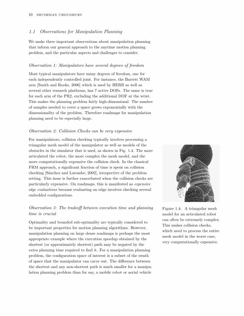


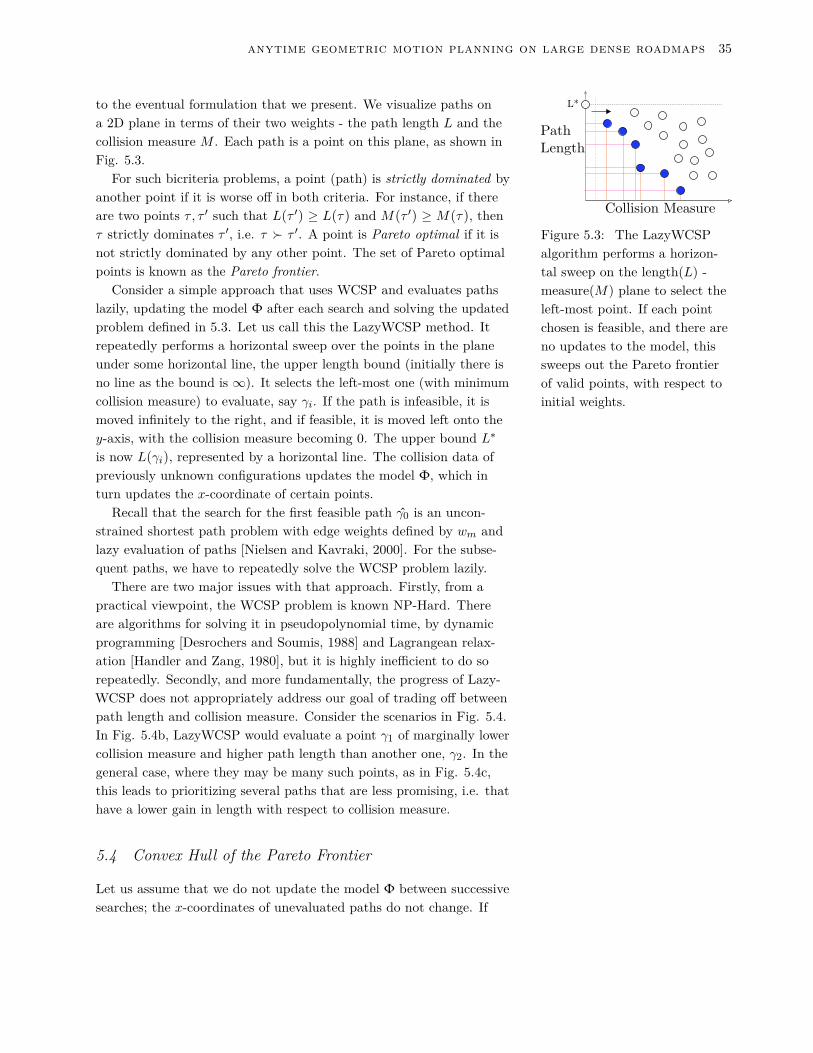


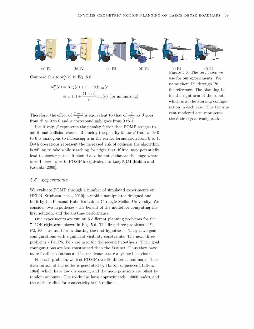


![RBaker Thesis1] Copy](https://static.documents.pub/doc/80x56/577d21c91a28ab4e1e95e3e9/rbaker-thesis1-copy.jpg)


![Exploiting Robotic Swarm Characteristics for Adversarial ...ri.cmu.edu/wp-content/uploads/2017/08/Masters_Thesis-Sanghvi.pdf · One approach based on localized Voronoi diagrams [22]](https://static.documents.pub/doc/80x56/5f073a3f7e708231d41bf19e/exploiting-robotic-swarm-characteristics-for-adversarial-ricmueduwp-contentuploads201708mastersthesis-.jpg)