Microprocessors and Microsystems 41 (2016) 12–28

Contents lists available at ScienceDirect

Microprocessors and Microsystems

journal homepage: www.elsevier.com/locate/micpro

Anytime system level verification via parallel random exhaustive

hardware in the loop simulation�

Toni Mancini∗, Federico Mari, Annalisa Massini, Igor Melatti, Enrico Tronci

Computer Science Department, Sapienza University of Rome, Italy

a r t i c l e i n f o

Keywords:

Model Checking of Hybrid Systems

Model checking driven simulation

Hardware in the loop simulation

a b s t r a c t

System level verification of cyber-physical systems has the goal of verifying that the whole (i.e., software +

hardware) system meets the given specifications. Model checkers for hybrid systems cannot handle sys-

tem level verification of actual systems. Thus, Hardware In the Loop Simulation (HILS) is currently the

main workhorse for system level verification. By using model checking driven exhaustive HILS, System

Level Formal Verification (SLFV) can be effectively carried out for actual systems.

We present a parallel random exhaustive HILS based model checker for hybrid systems that, by simulating

all operational scenarios exactly once in a uniform random order, is able to provide, at any time during

the verification process, an upper bound to the probability that the System Under Verification exhibits an

error in a yet-to-be-simulated scenario (Omission Probability).

We show effectiveness of the proposed approach by presenting experimental results on SLFV of the In-

verted Pendulum on a Cart and the Fuel Control System examples in the Simulink distribution. To the

best of our knowledge, no previously published model checker can exhaustively verify hybrid systems of

such a size and provide at any time an upper bound to the Omission Probability.

© 2015 Elsevier B.V. All rights reserved.

c

f

u

f

a

b

t

m

p

n

s

s

u

n

c

t

n

1. Introduction

The cost for fixing a design error in a system becomes larger

and larger as the design proceeds from the requirement analysis

to the implementation (see, e.g., [2, Chapter 1]) since the later in

the design phase an error is detected the more reworking it may

trigger. The above observation has motivated the development of

methods and tools to verify correctness of a system already in the

early phases of its design, namely during the requirement analysis

or during the functional specification phases. The goal of all such

approaches is to catch design errors well before the system imple-

mentation begins.

Of course, all such approaches are model based, that is they

work on a model describing the system behaviour since no sys-

tem implementation exists in the early design phases. Accordingly,

System Verification is carried out by simulating a system model and

analysing its behaviour under a suitable set of simulation scenarios.

For example, in a digital hardware setting, model based ap-

proaches have been used since a long time. In fact, even before

� This paper is an extended and revised version of [1].∗ Corresponding author.

E-mail addresses: tmancini@di.uniroma1.it (T. Mancini), mari@di.uniroma1.it

(F. Mari), massini@di.uniroma1.it (A. Massini), melatti@di.uniroma1.it (I. Melatti),

tronci@di.uniroma1.it (E. Tronci).

u

t

e

http://dx.doi.org/10.1016/j.micpro.2015.10.010

0141-9331/© 2015 Elsevier B.V. All rights reserved.

onsidering going to silicon, a heavy simulation activity is per-

ormed, aimed at verifying that the system model (defined, e.g.,

sing Verilog, VHDL or SystemC1) meets the system requirements

or most (possibly all) uncontrollable inputs (that is, primary inputs

nd faults the system is expected to withstand).

Along the same line of reasoning, in a purely software setting,

efore generating low level code, model based approaches are used

o verify that the software model (defined, e.g., using AADL [3,4])

eets the given requirements.

If all possible simulation scenarios are considered, then we can

rove correctness of the system (i.e., absence of simulation sce-

arios violating the system requirements), otherwise we can only

how that the system design is faulty (by exhibiting a simulation

cenario violating the system requirements). In other words, a sim-

lation campaign that does not consider all possible simulation sce-

arios can only show that the system design has a bug. To show

orrectness of the system design we need an exhaustive simula-

ion campaign, that is one considering all possible simulation sce-

arios. A verification approach able to show system correctness is

sually referred to as formal verification. One of the most successful

echniques to carry out formal verification is Model Checking (see,

.g., [5]).

1 http://www.mentor.com/products/fv/hdl_designer/

T. Mancini et al. / Microprocessors and Microsystems 41 (2016) 12–28 13

a

c

i

t

o

s

b

s

s

m

a

w

s

s

s

C

i

b

a

a

w

c

h

s

i

c

T

c

t

m

a

t

d

a

m

a

e

f

H

w

t

e

b

a

t

1

n

l

a

s

a

t

d

i

v

a

u

s

a

m

(

f

t

b

t

o

e

p

t

fi

v

f

l

a

s

a

d

o

w

b

s

p

d

m

d

i

y

P

f

r

h

n

t

e

a

c

1

s

The need for model checking stems from the high cost that

bug may have for certain systems. This is the case for mission

ritical systems, that is, systems for which a system malfunction-

ng may entail loss of money, as well as for safety critical systems,

hat is, systems for which a system malfunctioning may entail loss

f human lives. Examples of mission critical systems are: decision

upport systems, satellites, processors (e.g., the infamous P5 FDIV

ug costed about $475 million to INTEL). Examples of safety critical

ystems are: railway interlocking, avionics control software.

Many Cyber-Physical Systems (CPSs) are indeed mission or

afety critical systems. Accordingly, in this paper we focus on for-

al verification techniques for CPSs.

A CPS consists of hardware (e.g., motors, electrical circuits, etc.)

nd software components. Thus, in order to verify a CPS design,

e need methods and tools that can model and effectively support

imulation of hardware as well as software components.

From a formal point of view, CPSs can be modelled as hybrid

ystems (see, e.g., [6] and citations thereof). Many Model Based De-

ign software tools offer support for modelling and simulation of

PSs. Well known examples are Simulink2, VisSim3 and Model-

ca4. All such tools take as input a (mathematical) model of the

ehaviour of the CPS along with a simulation scenario and provide

s output the time evolution (trace or simulation run) of the system

t hand.

System Level Verification of CPSs aims at verifying that the

hole (i.e., software + hardware) system meets the given specifi-

ations. System Level Formal Verification (SLFV) has the goal of ex-

austively verifying that the above holds for all possible operational

cenarios.

For digital circuits, formal verification is usually carried out us-

ng model checking techniques (e.g., see [7]). Unfortunately, model

heckers for hybrid systems cannot handle SLFV of real world CPSs.

hus, HILS is currently the main workhorse for system level verifi-

ation of CPSs, and is supported by model based design tools (e.g.,

he previously mentioned Simulink, VisSim and Modelica).

In HILS, the actual software reads/sends values from/to mathe-

atical models (simulation) of the physical systems (e.g., engines,

nalog circuits, etc.) it will be interacting with. Notwithstanding

he word hardware, in HILS the only hardware present is the one

evoted to support the system simulation, that is: computational

nd communication devices. This is because HILS is used in a

odel based design setting to validate the system design before

ny hardware is built (the whole goal of model based design). For

xample, Simulink, VisSim, Modelica, ESA Satellite Simulation In-

rastructure SIMULUS5 all provide simulation software supporting

ILS, where the only hardware involved is just the computer on

hich the simulator is actually running.

Simulation can be very time consuming. Accordingly, in order

o reduce system design time, Opal-RT6 and dSpace7 among oth-

rs provide modelling and simulation software along with FPGA-

ased hardware to support real-time simulation. We note that in

ll cases the only hardware present in HILS is the one supporting

he simulation itself.

.1. Motivations

SLFV is an exhaustive HILS where all relevant simulation sce-

arios are considered. Using a parallel model checking driven

2 http://www.mathworks.com.3 http://www.vissim.com.4 http://www.modelica.org.5 http://www.esa.int/Our_Activities/Operations/gse/ESA_operations_software_

icensable_products_-_overview .6 http://www.opal-rt.com/about-hardware-loop-simulation .7 https://www.dspace.com/en/inc/home.cfm .

o

s

c

a

t

j

i

s

pproach, exhaustive HILS enables formal verification of actual

ystems. Examples of such systems are the Inverted Pendulum on

Cart (IPC) and the Fuel Control System (FCS) in the Simulink dis-

ribution (see Section 6.1.1).

Considering that parallel exhaustive HILS based SLFV may take

ays of computation (e.g., see [8]), from a practical point of view

t would be very useful to have available at any time during the

erification process, quantitative information about the degree of

ssurance attained. Such an information would enable us to eval-

ate if it is worth to continue the verification activity, or instead

top it since the degree of assurance attained can be considered

dequate for the application at hand (graceful degradation).

The above considerations suggest looking for a HILS based

odel checking approach satisfying the following requirements:

i) it is parallel, in order to make exhaustive HILS computationally

easible; (ii) it is exhaustive, since our focus is SLFV; (iii) it is any

ime, to support graceful degradation.

The work in [9] presents a Propositional Satisfiability (SAT)

ased model checker for finite state systems which returns, at any

ime during the verification process, the coverage (i.e., the fraction

f operational scenarios verified so far). Unfortunately, while cov-

rage measures the amount of verification work done, it does not

rovide any information about the degree of assurance attained by

he verification process. This is because formal verification aims at

nding hard to find errors, i.e., errors that were not detected while

erifying operational scenarios designed by experts. As a result,

ormal verification addresses the search of errors that we are un-

ikely to consider. For this reason, we can model the problem as an

dversary system, that is a system where, knowing our verification

trategy, the adversary places the error in operational scenarios we

re less likely to visit. In such a framework, any deterministic or-

ering of the operational scenarios would not increase the degree

f assurance until the end of the verification. In fact, the adversary

ould choose to place the single error in the last scenario picked

y the verification procedure.

To provide a formally sound information about the degree of as-

urance attained by the verification process, approaches have been

roposed which verify the operational scenarios in a random or-

er. In particular, the work in [10] presents a Monte-Carlo based

odel checker for finite state systems that provides, at any time

uring the verification process, an upper bound to the probabil-

ty that the System Under Verification (SUV) exhibits an error in a

et-to-be-simulated scenario (Omission Probability). The Omission

robability (OP) provides indeed the information we are looking

or. Unfortunately, while Monte-Carlo based approaches guarantee

andomness (thereby enabling OP computation) they are not ex-

austive (within a finite time).

To the best of our knowledge, no model checker is available,

either for finite state systems nor for hybrid systems, which, at

he same time, is both random and exhaustive, thereby enabling

ffective anytime SLFV. In this paper we advance the state of the

rt by presenting a parallel random exhaustive HILS based model

hecker along with experimental results showing its effectiveness.

.2. Main contribution

Our System Under Verification (SUV) is a Hybrid System (e.g.,

ee [6] and citations thereof) whose inputs belong to a finite set

f uncontrollable events (disturbances) modelling failures in sen-

ors or actuators, variations in the system parameters, etc. We fo-

us on deterministic systems (the typical case for control systems)

nd model nondeterministic behaviours (such as faults) with dis-

urbances. Accordingly, in our framework, a simulation scenario is

ust a finite sequence of disturbances and a simulation campaign

s a finite sequence of simulation instructions (namely: save a

imulation state, restore a saved simulation state, remove a saved

14 T. Mancini et al. / Microprocessors and Microsystems 41 (2016) 12–28

i

r

W

1

t

s

s

o

a

e

a

F

i

(

t

i

t

u

t

e

s

1

c

i

p

s

t

t

u

b

o

s

2

w

p

o

v

n

2

(

d

A

a

(

i

e

n

d

t

o

D

c

simulation state, inject a disturbance, advance the simulation of a

given time length).

A system is expected to withstand all disturbance sequences

that may arise in its operational environment. Correctness of a sys-

tem is thus defined with respect to such admissible disturbance

sequences. In our setting, the set of admissible disturbance se-

quences (disturbance model) can be defined as the language ac-

cepted by a suitable Finite State Automaton, which in turn can

be defined using the modelling language of any finite state model

checker.

In such a framework we address Bounded SLFV of safety prop-

erties. That is, given a time step τ (time quantum between dis-

turbances) and a time horizon T = τh we return PASS if there

is no admissible disturbance sequence of length h and time step

τ that violates the given safety property. We return FAIL, along

with a counterexample, otherwise. Therefore, SLFV is an exhaustive

(with respect to admissible disturbance sequences) HILS. In other

words, we are aiming at (black box) bounded model checking where

the SUV behaviour is defined by a simulator (Simulink in our

examples).

In such a setting, our main contribution can be summarised

as follows. We present an anytime parallel random exhaustive HILS

based model checker that effectively conjugates exhaustiveness

with randomness, thereby enabling the computation of the Omis-

sion Probability.

While a simulation run for digital hardware takes order of mil-

liseconds on a normal desktop computer, in our setting a simu-

lation run takes order of seconds since it entails heavy numer-

ical computations aimed at solving a system of many Ordinary

Differential Equations (modelling the hardware components of the

CPS). Indeed (see Section 6) simulation of operational scenarios

takes almost 100% of the overall verification time. Resting on such

observation we build on the SLFV approach discussed in [8]. In

particular:

1. From the disturbance model we generate all admissible sim-

ulation scenarios and evenly split them into disjoint sets

(slices).

2. For each slice, we compute a highly optimised simula-

tion campaign that exploits simulator save/restore/remove

commands in order to save on the simulation time while

scheduling execution of all simulation scenarios exactly once

and in a uniform random order. This guarantees exhaustive-

ness and allows us to compute, at any time during the veri-

fication process, an upper bound to the OP.

3. We run simulation campaigns in parallel. This guarantees a

very efficient parallelism, since no communication among

processes is needed. This step is supported by simulation

tools (Simulink in our case study).

We also show that, thanks to the fact that we have first gen-

erated all admissible simulation scenarios, attaining point 2 above

(i.e., anytime OP computation) can be done in a not-too-complicated

(from both technical and computational points of view) and non-

invasive way, by simply introducing a new module into the work-

flow of [8] that seamlessly interoperates with the others.

1.3. Summary of experimental results

We implemented our approach and present (Section 6) exper-

imental results on two case studies, namely the Inverted Pendu-

lum on a Cart (IPC) and the Fuel Control System (FCS) examples in

the Simulink distribution. Overall, we compute optimised simula-

tion campaigns under four operational environments (disturbance

models), which entail from 3 208 276 to 35 641 501 simulation

scenarios.

Each processor (actually, a core of a 8-core machine) runs an

nstance of our (random) simulation campaign computation algo-

ithm and takes as input a slice of our set of simulation scenarios.

e present experimental results with 16, 32, 64 machines totalling

28, 256, 512 parallel processes. Our approach takes negligible

ime to generate an optimised simulation campaign for a given

lice, with respect to the time needed to actually execute the

imulation campaign (e.g., minutes vs. hours, see Section 6).

Our experimental results show that, by exploiting parallelism,

ur random exhaustive simulation campaigns effectively counter-

ct the simulation time overhead due to randomisation. The above

nsures feasibility of our parallel random exhaustive approach for

ctual systems, such as the Inverted Pendulum on a Cart (IPC) and

uel Control System (FCS) examples in the Simulink distribution.

As for the Omission Probability (OP), the worst case scenario

s when just one error trace is present. Our experimental results

Section 6.6) show that, even in such a case, our upper bound to

he OP decreases about linearly with respect to the coverage, that

s the fraction of scenarios simulated. This is the best one can hope

o obtain in our setting.

Finally, simulation of scenarios in random order allows us to

se the coverage as a reliable estimator for the completion time of

he whole verification task. Our experimental results show that the

rror in the completion time estimation decreases quickly with re-

pect to coverage.

.4. Paper outline

Section 2 gives background notions to make our paper self-

ontained. Section 3 presents our formal framework, by formalis-

ng the notion of OP and by providing an upper bound for it, com-

utable from the number of the yet-to-be-simulated traces in each

lice. Section 4 outlines our algorithm which enables the compu-

ation, from a sequence (slice) of disturbance traces, a highly op-

imised simulation campaign which simulates the input traces in

niform random order and exploits the save/restore/remove capa-

ilities of the simulator. Section 5 is devoted to the formal proofs

f our results. Finally, Section 6 presents experimental results as-

essing effectiveness of our approach.

. Background and preliminaries

In this section we give some background notions. Unless other-

ise stated, all definitions are based on [8,11,12]. Throughout the

aper, we use R≥0 for the set of non-negative reals, R

+ for the set

f strictly positive reals, and Bool = {0, 1} for the set of Boolean

alues (0 for false and 1 for true). N+ denotes the set of positive

atural numbers.

.1. Modelling the operational environment

Our System Under Verification (SUV) is a Discrete Event System

DES), namely a continuous time Input-State-Output deterministic

ynamical system [11] whose inputs are discrete event sequences.

discrete event sequence (Definition 1) is a function u(t) associ-

ting to each (continuous) time instant t ∈ R≥0 a disturbance event

or, simply, disturbance). Disturbances, encoded by natural numbers

n the interval [0, d] (for a given d ∈ N+), represent uncontrollable

vents (e.g., faults). We use event 0 to represent the event carrying

o disturbance. As no system can withstand an infinite number of

isturbances within a finite time, we require that, in any time in-

erval of finite length, a discrete event sequence u(t) differs from 0

nly in a finite number of time points (Fig. 1a).

efinition 1 (Discrete event sequence). Let d ∈ N+. A dis-

rete event sequence over the natural interval [0, d] is a

T. Mancini et al. / Microprocessors and Microsystems 41 (2016) 12–28 15

a b c

Fig. 1. (a) A discrete event sequence (d = 3); (b) Our SUV embedding a monitor; (c) The SUV monitor output.

a b c d

Fig. 2. (a) Disturbance model; (b) CMurphi-based disturbance generator; (c) Gener-

ated sequence of disturbance traces (d = 3, h = 6); (d) The discrete event sequence

associated to the trace in the black rectangle in part (c), given time quantum τ .

f{w

c

t

c

D

i

<

s

r

D

ω

t

ω

a

a

(

c

a

e

t

D

b

τa

a

=

(

q

o

�

R

N

i

a

c

v

fi

i

n

p

E

t

(

t

c

a

z

f

d

unction u : R≥0 → [0, d] such that, for all t ∈ R

≥0, the set

t ∈ R≥0 | 0 ≤ t ≤ t and u(t) �= 0

}has finite cardinality. We denote

ith Ud the set of discrete event sequences over [0, d] (following

ontrol engineering notation for input functions to dynamical sys-

ems, see e.g. [11]).

In Definitions 2 and 3 we specify the concepts of restriction and

oncatenation, respectively, for functions belonging to Ud .

efinition 2. Let Ud be the set of discrete event sequences over the

nterval [0, d]. Given a function u ∈ Ud and two real numbers 0 ≤ t1

t2, we denote with u|[t1,t2) the function u|[t1,t2) : [t1, t2) → [0, d],

uch that u|[t1,t2)(t) = u(t) for all t ∈ [t1, t2). We denote U [t1,t2)

dthe

estriction of Ud to the domain [t1, t2).

efinition 3. Assume that t1, t2, t3 ∈ R≥0 such that t1 < t2 < t3. If

∈ U [t1,t2)

dand ω′ ∈ U [t2,t3)

d, their concatenation, denoted as ωω′, is

he function ω ∈ U [t1,t3)

ddefined as:

˜ (t) ={ω(t) if t ∈ [t1, t2)ω′(t) if t ∈ [t2, t3)

System level verification follows an Assume-Guarantee approach

imed at showing that the SUV meets its specification (Guarantee)

s long as the SUV operational environment behaves as expected

Assume). In this work we focus on bounded system level verifi-

ation. As a consequence, we model (Definition 4) the SUV oper-

Fig. 3. Exam

tional environment as the sequence of disturbances our SUV is

xpected to withstand within a finite time horizon, and we bound

he time quantum between two consecutive disturbances.

efinition 4 (Disturbance trace). Let h, d ∈ N+. An (h, d) distur-

ance trace δ is a finite sequence δ : [0, h − 1] → [0, d]. Given

∈ R+ (time quantum), an (h, d) disturbance trace δ is univocally

ssociated to a discrete event sequence uτδ, defined as follows: for

ll t ∈ R≥0, if there exists j ∈ [0, h − 1] such that t = τ j, then uτ

δ(t)

δ(j), else uτδ(t) = 0 (no disturbance).

Thus, a disturbance trace δ defines an operational scenario

namely, uτδ

) for our SUV. Fig. 2d shows the discrete event se-

uence associated to a disturbance trace. We represent our SUV

perational environment as a finite set of (h, d) disturbance traces

= {δ0, . . . , δn−1}, since Uτ�

= {uτδ0

, . . . , uτδn−1

} (for a given τ ∈+) defines the operational scenarios our SUV should withstand.

ote that, by taking h large enough (as in Bounded Model Check-

ng BMC) and τ small enough (to faithfully model our SUV oper-

tional scenarios), we can achieve any desired precision. On such

onsiderations rests the effectiveness of the approach.

As it is typically infeasible to define a SUV operational en-

ironment by explicitly listing all its disturbance traces, we de-

ne an operational environment with a disturbance model which

s in turn defined as the language accepted by a suitable fi-

ite state automaton. The following example illustrates this

oint.

xample 1. Consider a disturbance model consisting of one dis-

urbance (namely, a fault) which is always recovered within 4 s

i.e., 4 seconds). Let us assume that between two consecutive dis-

urbances (faults) there must be at least 5 s and that disturbances

an arise only at time steps multiple of τ = 1 s (time quantum). We

lso assume that the verification time horizon is set to 6 s.

In Fig. 3a we show disturbance traces represented as strings of

eros (no disturbance) and ones (disturbance), with time flowing

rom left to right. The 8 strings terminated by denote all the

isturbance traces accepted by the disturbance model (admissible

ple 1.

16 T. Mancini et al. / Microprocessors and Microsystems 41 (2016) 12–28

a b c d e

Fig. 4. Parallel HILS based dSLFV [8]: k parallel processes are run on m multi-core machines (we show a possible deployment with machines having c cores each, i.e.,

k = mc).

o

h

D

M

B

2

fi

D

t

(

c

o

a

d

h

b

d

2

d

i

S

i

e

r

a

t

(

t

disturbance traces). The 14 strings terminated by are the shortest

non-admissible sequences of disturbances, that is disturbance se-

quences that cannot be extended to admissible disturbance traces.

Fig. 3b shows the pseudo-code for a finite state automaton

recognising such a language.

We define a finite state automaton for a disturbance model us-

ing the modelling language of a finite state model checker (namely,

CMurphi [13]), along the lines of [8].

2.2. Modelling the property to be verified

Along the lines of [14], we model the property to be verified

with a continuous-time monitor which observes the state of the

system to be verified and checks whether the property under ver-

ification is satisfied (Fig. 1b). The output of the monitor is 0 as

long as the property under verification is satisfied and becomes

and stays 1 (sustain) as soon as the property fails, thus ensuring

that we never miss a property failure report, even when sampling

the monitor output only at discrete time points (Fig. 1c). The use

of monitors gives us a flexible approach to model the property

to be verified. In particular, it is easy to model bounded safety

and bounded liveness properties as monitors. Figs. 8 and 9 show

the Simulink/Stateflow representations of our two case studies (In-

verted Pendulum on a Cart and Fuel Control System, respectively),

along with their property monitors (see Section 6).

2.3. Modelling the SUV

Since the monitor output is all we need to carry out our ver-

ification task, we can model our SUV along with the property to

be verified as a DES with an embedded monitor (Fig. 1b). We call

Monitored Discrete Event System (MDES) such a DES.

According to our black-box approach to SUV modelling, given

a time quantum τ ∈ R+, Definition 5 formalises an (h, d) MDES

as a function H associating, to each (h, d) disturbance trace δ, a

Boolean value H(δ) representing the output of the SUV monitor

at time T = τh (the time horizon), when the system (starting from

its initial state) is given as input the discrete event sequence uτδ(t)

associated to δ. For any disturbance trace δ, H(δ) is 1 (error) if and

nly if uτδ(t) violates the property under verification within time

orizon T = τh (with the SUV starting from its initial state).

efinition 5. ((h, d) Monitored DES) Let h, d ∈ N+. A (h, d)

onitored Discrete Event System (MDES) is a function H :

([0, h − 1] → [0, d]) → Bool mapping all (h, d) disturbance traces to

oolean values.

.4. System Level Formal Verification (SLFV)

Definition 6 formalises our bounded System Level Formal Veri-

cation problem.

efinition 6. A System Level Formal Verification (SLFV) problem is a

uple P = (h, d, �, H) where: h, d ∈ N+, � = {δ0, . . . , δn−1} is an

h, d) set of disturbance traces, and H is a (h, d) MDES.

The answer to SLFV problem P is FAIL if there exists a distur-

bance trace δ in � such that H(δ) = 1 (in such a case also the

ounterexample δ is returned), PASS otherwise.

Note that, notwithstanding the fact that the number of states

f our SUV is infinite and we are in a continuous time setting, to

nswer a SLFV problem we only need to check a finite number of

isturbance traces. This is because we are bounding: (a) our time

orizon to T = τh, and (b) the set of time points at which distur-

ances can take place, by taking τ as the time quantum among

isturbance events.

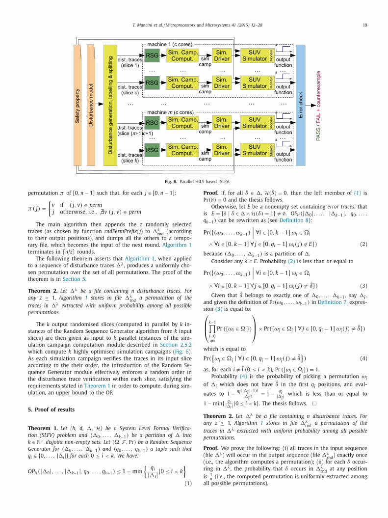
.5. Parallel HILS based deterministic SLFV

In the black-box parallel approach shown in [8], the MDES Hefining our SUV (plus the property to be verified) is defined us-

ng the modelling language of a suitable simulator (e.g., MatLab and

tateflow for Simulink). The answer to a SLFV problem (h, d, �, H)

s computed by simulating each operational scenario δ in the op-

rational environment �, thus by performing an exhaustive (with

espect to �) Hardware In the Loop Simulation (HILS). The over-

ll workflow is shown in Fig. 4 and described in the remainder of

his section. We will refer to this approach as Deterministic SLFV

dSLFV), where the word “deterministic” stems from the fact that

he disturbance traces are verified in a deterministic order.

T. Mancini et al. / Microprocessors and Microsystems 41 (2016) 12–28 17

Fig. 5. Labelled disturbance traces and optimised simulation campaign.

2

w

t

g

δa

l

o

c

s

m

l

t

t

t

d

c

i

s

i

t

w

v

d

�

e

n

2

s

a

S

a

d

H

t

c

a

r

s

i

r

r

a

s

s

i

w

u

t

b

m

b

i

3

f

s

c

3

i

i

p

s

N

b

m

P

I

r

o

i

D

e

b

n

f

.5.1. Disturbance trace generation and splitting

Our CMurphi-based trace generator (see Section 2.1 and Fig. 4a)

orks in Depth-First Search (DFS) mode, and, given the set of dis-

urbances, produces a sequence � of n disturbance traces. Each

enerated trace δ in � is annotated with labels and is of the form

= (l0, d0, l1, d1, . . . , lh−1, dh−1, lh), where δ = (d0, . . . , dh−1) is

sequence of disturbances satisfying the disturbance model and

0, . . . , lh belong to a countable set of labels L.

Labels are defined by an injective map λ from finite sequences

f disturbances (including the empty sequence) to L. Label l0 is

ommon to all traces and it is associated to the simulator initial

tate. Prefixes of disturbance sequences (d0, . . . , dp−1) common to

ultiple disturbance traces in � are followed by the same label

p = λ(d0, . . . , dp−1). Fig. 5a shows a short sequence of labelled dis-

urbance traces.

Labels identifying common disturbance prefixes are essential in

he efficient computation of optimised simulation campaigns. Note

hat, given that our CMurphi-based generator runs in DFS mode,

isturbance traces can be labelled at no additional computational

ost during generation. Trace labelling during generation greatly

ncreases the efficiency of the simulation campaign optimiser, as

hown in [8].

In the following, we will use δλ instead of δ (respectively, �λ

nstead of �) when we want to emphasise that a trace δ is anno-

ated (respectively, all traces in set � are annotated) with labels, or

hen we need such labels. In order to enable parallel verification

ia k ∈ N+ processes, we evenly partition the sequence of labelled

isturbance traces �λ into k ∈ N+ sequences of disturbance traces

λ0 , . . . , �λ

k−1(called slices).

The splitting process produces slices containing n/k traces

ach, except the last slice, which may contain fewer traces if n is

ot a multiple of k.

.5.2. Computation of optimised simulation campaigns

In the next phase of the workflow in Fig. 4, we use the k

lices �λ0 , . . . ,�λ

k−1generated so far to compute, independently

nd in parallel, k highly optimised simulation campaigns (Fig. 4b).

uch simulation campaigns can be simulated, again independently

nd in parallel, using k simulators, each one running (e.g., on a

ifferent core of a bunch of multi-core machines) a model for

(Fig. 4c–d).

The answer to the SLFV problem is FAIL if one of the simula-

ion campaigns raises the simulator output function to 1 (in this

ase the disturbance trace δ which raised the error is returned as

counterexample, see Fig. 4e). The answer is PASS otherwise.

Each simulator accepts four basic commands: store, load, free,

un. Command store(l) stores in memory the current state of the

imulator and labels with l such a state. Command load(l) loads

nto the simulator the stored state labelled with l. Command free(l)

emoves from the memory the state labelled with l. Command

un(e, t) (with e ∈ [0, d] and t ∈ R+) injects disturbance e and then

dvances the simulation of time t. A simulation campaign is thus a

equence of simulator commands.

The simulation campaign χ i (0 ≤ i < k) computed from input

lice �λi

steers the simulator as to execute all disturbance traces

n �λi

according to their order in the slice (this is the reason why

e refer to this approach as Deterministic SLFV).

Each disturbance trace is executed as if starting from the sim-

lator initial state. However, by using commands store and load,

he optimiser avoids revisiting simulation states as much as possi-

le (as in explicit model checking). Using command free the opti-

iser removes from the simulator memory states that will never

e needed in the remaining part of the simulation campaign. This

s needed since each state may require many KB of memory (150–

00 KB in the case studies presented in this paper).

Fig. 5b shows the optimised simulation campaign computed

rom the sequence of labelled disturbance traces in Fig. 5a, in the

imple case where we ignore any limit on number of states that

an be kept simultaneously stored in the simulator memory.

. Omission Probability

This section formally defines the notion of Omission Probabil-

ty (OP) (Definitions 7 and 8) and provides an upper bound for

t, which can be computed anytime during the parallel verification

rocess from the number of the yet-to-be-simulated traces in each

lice (Theorem 1).

otation 1 (Set of permutations of a set). Let � = {δ0, . . . , δn−1}e a finite non-empty set. We denote with Perm(�) the set of per-

utations of elements of �:

erm(�) = {(θ0, . . . , θn−1) | (∀i ∈ [0, n − 1] θi ∈ �)

∧(∀i, j ∈ [0, n − 1] i �= j → θi �= θ j)}

f � = (δ0, . . . , δn−1) ∈ Perm(�) we write also �(i) for δi.

A Random Sequence Generator (RSG) models the extraction of a

andom permutation from a given finite non-empty set (which, in

ur case, will be the set of admissible disturbance traces �). This

s formalised in Definition 7.

efinition 7 (Random Sequence Generator). Let � be a finite non-

mpty set. A Random Sequence Generator (RSG) for � is a proba-

ility space (,F , Pr), where:

• (the space of outcomes) is the set of permutations of �, that

is = Perm(�).

• F (the space of events) is the set of subsets of , that is: F =2 = {E | E⊆}.

• Pr : F → [0, 1] is a probability measure such that, for all ω ∈ ,

Pr(ω) = 1|�|! . That is, permutations of � are extracted with

uniform probability. Since is countable (actually finite),

the probability of any event E ∈ F is defined as Pr(E) =∑ω∈E Pr(ω).

Let (�0, . . . , �k−1) be a partition of � into k ∈ N+ disjoint

on-empty sets. For any 0 ≤ i < k, let (i,Fi, Pri) be a RSG

or �i. A Random Sequence Generator for (�0, . . . , �k−1) is a

18 T. Mancini et al. / Microprocessors and Microsystems 41 (2016) 12–28

g

o

O

t

s

4

e

s

c

S

s

c

fi

o

S

S

p

a

b

r

t

w

t

(

S

p

u

u

d

m

t

i

(

i

w

m

d

t

m

t

p

b

m

t

m

m

p

S

(

s

1

a

d

s

r

probability space (,F , Pr), where: = ×k−1i=0

i, F = ×k−1i=0

Fi and,

for each event E0 × · · · × Ek−1 ∈ F (Ei ∈ Fi for each 0 ≤ i < k),

P(E0 × · · · × Ek−1) = ∏k−1i=0 Pri(Ei).

Note that, by Definition 7, a RSG for a partition (�0, . . . , �k−1)

of � models the extraction of k permutations of, respectively,

�0, . . . , �k−1. For all 0 ≤ i < k, the extracted permutation of �i is

chosen uniformly among all possible permutations of �i. Also, the

k permutations are extracted independently from each other.

Definition 8 defines the probability of omitting the simulation

of a trace δ ∈ � containing an error (i.e., H(δ) = 1) when the veri-

fication process has already examined qi disturbance traces, where

qi ∈ {0, . . . , |�i|}, from a random permutation of slice �i, for all

0 ≤ i < k. Thus qi represents the state of advancement of the com-

putation on the ith slice �i. Hence (q0, . . . , qk−1) defines the state

of advancement (stage) of the computation on all slices. We denote

this probability as Omission Probability (OP).

Definition 8 (Omission Probability). Let (h, d, �, H) be a System

Level Formal Verification (SLFV) problem and (�0, . . . , �k−1) be a

partition of � into k ∈ N+ disjoint non-empty sets. Let (,F , Pr)

be a RSG for (�0, . . . , �k−1), and (q0, . . . , qk−1) a tuple such that

qi ∈ {0, . . . , |�i|} for each 0 ≤ i < k.

The Omission Probability (OP) for (�0, . . . , �k−1) at stage

(q0, . . . , qk−1), is defined as:

OPH(|�0|, . . . , |�k−1|, q0, . . . , qk−1)

= Pr

({(ω0, . . . , ωk−1)| ∀i ∈ [0, k − 1] ωi ∈ i ∧

AB((ω0, . . . , ωk−1), (q0, . . . , qk−1))

})where:

• AB is defined as A((ω0, . . . , ωk−1), (q0, . . . , qk−1)) ∧B((ω0, . . . , ωk−1), (q0, . . . , qk−1))

• A (After) is: A((ω0, . . . , ωk−1), (q0, . . . , qk−1)) = ∃i ∈ [0, k −1] ∃ j ∈ [qi, |�i|] H(ωi( j)) = 1;

• B (Before) is: B((ω0, . . . , ωk−1), (q0, . . . , qk−1)) = ∀i ∈[0, k − 1] ∀ j ∈ [0, qi − 1] H(ωi( j)) = 0.

In Definition 8, formula A (After) states that there exists a yet-

to-be-simulated trace δ (some trace j ≥ qi of some slice i) contain-

ing an error, i.e., such that H(δ) evaluates to 1. Formula B (Before)

states that none of the already simulated traces contains an error,

i.e., function H evaluates to 0 for all of them.

The following Theorem 1 gives an upper bound to the OP, after

having simulated qi randomly extracted traces from slice �i (for

each 0 ≤ i < k). In particular, Theorem 1 provides a bound to the

probability of omitting the simulation of a trace δ ∈ � containing

an error when the verification process has already examined qi dis-

turbance traces from the (the permutation of) slice �i (for all 0 ≤i < k). Importantly, the bound provided does not depend on H, i.e.,

it is independent of the system model. The proof of the theorem is

in Section 5.

Theorem 1. Let (h, d, �, H) be a SLFV problem and (�0, . . . , �k−1)

be a partition of � into k ∈ N+ disjoint non-empty sets. Let (,F , Pr)

be a Random Sequence Generator for (�0, . . . , �k−1) and (q0, . . . ,

qk−1) a tuple such that qi ∈ {0, . . . , |�i|} for each 0 ≤ i < k. We

have:

OPH(|�0|, . . . , |�k−1|, q0, . . . , qk−1) ≤ 1 − min

{qi

|�i| |0 ≤ i < k

}(1)

Note that the construction of the slices �0, . . . ,�k−1 from � is

non-deterministic (i.e., any partitioning of � would work), whereas,

for each slice, the selection of a permutation is a probabilistic pro-

cess, modelled as a RSG. Accordingly, Theorem 1 bounds the OP

using the worst case distribution, i.e., the distribution yielding the

reatest OP. From this stems the min function in the right member

f the inequality in Theorem 1.

Finally, we observe that, from Theorem 1, it follows that

PH(|�0|, . . . , |�k−1|, |�0|, . . . , |�k−1|) = 0, that is, our verification

ask terminates after max {|�i| | 0 ≤ i < k} parallel steps, having

imulated all traces in �.

. Enabling Omission Probability computation: random

xhaustive SLFV

Our disturbance trace generator (see Section 2.1) produces a

equence of disturbance traces �λ, whose order is deterministi-

ally chosen by the employed algorithm (in our case, Depth-First

earch (DFS)). As a consequence, no information about the Omis-

ion Probability (OP) can be inferred during the verification pro-

ess if the simulation campaign computed from each slice veri-

es the sequence of disturbance traces therein according to their

rder (as done by the Deterministic SLFV (dSLFV) approach of

ection 2.5), or according to any deterministic order, as argued in

ection 1.1.

From Section 3 it follows that it is possible to enable OP com-

utation (and hence, graceful degradation during the computation-

lly very expensive simulation phase) by simulating the distur-

ance traces within each slice in an order uniformly chosen at

andom.

Here we show how we can add support to OP computation in

he workflow of Fig. 4 in a not-too-complicated and non-invasive

ay, by introducing an additional step, in the parallel portion of

he workflow, which implements a Random Sequence Generator

RSG).

The new workflow, which we refer to as random exhaustive

LFV (rSLFV), is shown in Fig. 6. All slices are given as input, in

arallel, to instances the new Random Sequence Generator mod-

le, shown as Algorithm 1. The Random Sequence Generator mod-

le reads a sequence of disturbance traces and computes a ran-

om permutation of it, uniformly chosen among all possible per-

utations, thus implementing a RSG (Definition 7). We argue that

he introduction of the new Random Sequence Generator module

s non-too-complicated for what concerns both its implementation

Algorithm 1) and its computational viability (see Section 6.3). It

s also non-invasive, as it seamlessly interoperates with the dSLFV

orkflow of Section 2.5.

As the input sequence can be too large to be kept in main

emory, the Random Sequence Generator module implements a

isk-based multi-round algorithm (shown as Algorithm 1) which

akes efficiency into account by using, in each round, as much

ain memory as possible and by reading/writing the input/output

race files sequentially.

Let n = |�λ| be the number of disturbance traces in the in-

ut sequence. Given parameter z ∈ N+ for the maximum num-

er of disturbance traces which can be simultaneously stored in

ain memory, the algorithm, at each round r ≥ 1, selects the z

races which will have output positions in the interval [(r − 1)z,

in(n, rz − 1)].

The above selection is performed by computing the first z ele-

ents of a random permutation of the traces not yet in the out-

ut file �λrnd

, chosen uniformly among all possible permutations.

uch a permutation prefix is computed by function rndPermPrefix()

Algorithm 1, from line 20). Function rndPermPrefix() performs a

wap-based computation of a permutation of integers [0, |�λin| −

] (uniformly chosen at random) and interrupts the computation

s soon as the first z elements (see variable result) have been

etermined. During its operation, function rndPermPrefix() repre-

ents the partially computed permutation as an associative ar-

ay perm, which, at any step of the function execution, represents

T. Mancini et al. / Microprocessors and Microsystems 41 (2016) 12–28 19

Fig. 6. Parallel HILS based rSLFV.

p

π

t

t

r

t

t

s

t

T

a

t

p

s

s

u

w

A

a

q

t

r

u

5

T

t

k

G

q

O

P

P

i

q

P

b

P

a

s⎛⎜⎝w

P

a

o

u

1

T

a

t

p

P

(

(

r

i

a

ermutation π of [0, n − 1] such that, for each j ∈ [0, n − 1]:

( j) ={

v if ( j, v) ∈ permj otherwise, i.e., � ∃v ( j, v) ∈ perm

The main algorithm then appends the z randomly selected

races (as chosen by function rndPermPrefix()) to �λrnd

(according

o their output positions), and dumps all the others to a tempo-

ary file, which becomes the input of the next round. Algorithm 1

erminates in n/z rounds.

The following theorem asserts that Algorithm 1, when applied

o a sequence of disturbance traces �λ, produces a uniformly cho-

en permutation over the set of all permutations. The proof of the

heorem is in Section 5.

heorem 2. Let �λ be a file containing n disturbance traces. For

ny z ≥ 1, Algorithm 1 stores in file �λrnd

a permutation of the

races in �λ extracted with uniform probability among all possible

ermutations.

The k output randomised slices (computed in parallel by k in-

tances of the Random Sequence Generator algorithm from k input

lices) are then given as input to k parallel instances of the sim-

lation campaign computation module described in Section 2.5.2

hich compute k highly optimised simulation campaigns (Fig. 6).

s each simulation campaign verifies the traces in its input slice

ccording to the their order, the introduction of the Random Se-

uence Generator module effectively enforces a random order in

he disturbance trace verification within each slice, satisfying the

equirements stated in Theorem 1 in order to compute, during sim-

lation, an upper bound to the OP.

. Proof of results

heorem 1. Let (h, d, �, H) be a System Level Formal Verifica-

ion (SLFV) problem and (�0, . . . , �k−1) be a partition of � into

∈ N+ disjoint non-empty sets. Let (,F , Pr) be a Random Sequence

enerator for (�0, . . . , �k−1) and (q0, . . . , qk−1) a tuple such that

i ∈ {0, . . . , |�i|} for each 0 ≤ i < k. We have:

PH(|�0|, . . . , |�k−1|, q0, . . . , qk−1) ≤ 1 − min

{qi

|�i| |0 ≤ i < k

}(1)

roof. If, for all δ ∈ �, H(δ) = 0, then the left member of (1) is

r(∅) = 0 and the thesis follows.

Otherwise, let E be a nonempty set containing error traces, that

s E = {δ | δ ∈ � ∧ H(δ) = 1} �= ∅. OPH(|�0|, . . . , |�k−1|, q0, . . . ,

k−1) can be rewritten as (see Definition 8):

r({(ω0, . . . , ωk−1)

∣∣∣ ∀i ∈ [0, k − 1] ωi ∈ i

∧ ∀i ∈ [0, k − 1] ∀ j ∈ [0, qi − 1] ωi( j) �∈ E}) (2)

ecause (�0, . . . , �k−1) is a partition of �.

Consider any δ ∈ E. Probability (2) is less than or equal to

r({(ω0, . . . , ωk−1)

∣∣∣ ∀i ∈ [0, k − 1] ωi ∈ i

∧ ∀i ∈ [0, k − 1] ∀ j ∈ [0, qi − 1] ωi( j) �= δ}) (3)

Given that δ belongs to exactly one of �0, . . . , �k−1, say �i,

nd given the definition of Pr(ω0, . . . , ωk−1) in Definition 7, expres-

ion (3) is equal to:

k−1∏i=0i �=i

Pr ({ωi ∈ i})

⎞⎟⎠ × Pr({ωi ∈ i | ∀ j ∈ [0, qi − 1] ωi( j) �= δ})

hich is equal to

r({ωi ∈ i | ∀ j ∈ [0, qi − 1] ωi( j) �= δ

}) (4)

s, for each i �= i (0 ≤ i < k), Pr ({ωi ∈ i}) = 1.

Probability (4) is the probability of picking a permutation ωi

f �i

which does not have δ in the first qi

positions, and eval-

ates to 1 − qi(|�

i|−1)!

|�i|! = 1 − q

i|�i| which is less than or equal to

− min{ qi|�i| |0 ≤ i < k}. The thesis follows. �

heorem 2. Let �λ be a file containing n disturbance traces. For

ny z ≥ 1, Algorithm 1 stores in file �λrnd

a permutation of the

races in �λ extracted with uniform probability among all possible

ermutations.

roof. We prove the following: (i) all traces in the input sequence

file �λ) will occur in the output sequence (file �λrnd

) exactly once

i.e., the algorithm computes a permutation); (ii) for each δ occur-

ing in �λ, the probability that δ occurs in �λrnd

at any position

s 1n (i.e., the computed permutation is uniformly extracted among

ll possible permutations).

20 T. Mancini et al. / Microprocessors and Microsystems 41 (2016) 12–28

Algorithm 1 Random Sequence Generator.

t

m

t

p

P

w

r

r

Point (i) is immediate: at each round, z traces are appended to

�λrnd

, all the others are appended to �λtmp, which becomes the in-

put of the next round. Also, the algorithm terminates only if the

�λtmp produced at the previous round is empty.

To prove point (ii), for any p, q in [0, n − 1], we compute the

probability that trace δ having position p in the input sequence

(file �λ) will have position q in the output sequence (file �λrnd

).

We omit to prove that function rndPermPrefix(n,z) actu-

ally computes the first z elements of a permutation of the

integer interval [0, n − 1] uniformly selected at random, as

the function interrupts a well-known swap-based permuta-

tion algorithm as soon as the first z elements have been

determined.

Given that, at each round r ≥ 1, the main algorithm selects

he z input traces which will have output positions (r − 1)z to

in(n, rz − 1), δ is selected only at round rδ = (q + 1)/z. Thus,

he probability that δ, having input position p, will have output

osition q is:

r

((rδ−1⋂r=1

¬Er

)∩ Oq′

rδ

)(5)

here, for all r, ¬Er denotes the event “δ is not selected at round

” and Oq′rδ

denotes the event “δ is the q′th trace selected in round

δ ,” where q′ = (q − z(rδ − 1)).

By the chain rule, (5) becomes:

T. Mancini et al. / Microprocessors and Microsystems 41 (2016) 12–28 21

P

×

w

c

n

n

P

a

P

q

l

×

w

w

(

t

l

d

6

h

o

t

i

p

a

u

6

t

6

c

o

6

s

s

w

p

Fig. 7. Inverted Pendulum on a Cart (IPC) case study (from mathworks.com).

a

(

c

h

w

F

U

a

u

p

[

l

c

c

t

t

s

Dd

m

d

w

d

o

c

p

t

d

t

r

6

t

i

t

f

t

p

j

r

e

r

i

w

u

r (¬E1) × · · · × Pr(¬Erδ−1|¬Erδ−2, . . . ¬E1

)Pr

(Oq′

rδ|¬Erδ−1, . . . ¬E1

). (6)

For all 1 ≤ r ≤ rδ − 1:

Pr (¬Er|¬Er−1, . . . ¬E1) = n − z(r − 1) − 1

n − z(r − 1)× · · ·

× n − z(r − 1) − z

n − z(r − 1) − (z − 1)

here, for all 0 ≤ i < z, the ith factor is the number of ways we

an choose a trace different from δ out of n − z(r − 1) − i (where

− z(r − 1) is the number of traces still not selected at the begin-

ing of round r). The expression simplifies to:

r (¬Er|¬Er−1, . . . ¬E1) = n − zr

n − z(r − 1)

nd the product Pr (¬E1) × · · · × Pr(¬Erδ−1|¬Erδ−2, . . . ¬E1

)is:

r (¬E1) × · · · × Pr(¬Erδ−1|¬Erδ−2, . . . ¬E1

)=

rδ−1∏r=1

n − zr

n − z(r − 1)

= n − z(rδ − 1)

n. (7)

As for Pr

(O

q′rδ|¬Erδ−1, . . . ¬E1

), i.e., the probability that δ is the

′th selected trace in round rδ provided that it has not been se-

ected in previous rounds, it can be computed as:

n − z(rδ − 1) − 1

n − z(rδ − 1)× · · · × n − z(rδ − 1) − (q′ − 1)

n − z(rδ − 1) − (q′ − 2)

1

n − z(rδ − 1) − (q′ − 1)= 1

n − z(rδ − 1)(8)

here, for all 0 ≤ i < q′ − 1, the ith factor is the number of ways

e can choose a trace different from δ out of n − z(rδ − 1) − i

where n − z(rδ − 1) is the number of traces still not selected at

he beginning of round rδ). The last factor is the probability of se-

ecting δ (still unselected) out of n − z(rδ − 1) − (q′ − 1) traces.

By (7) and (8), probability (6) evaluates to 1n , which is indepen-

ent of p and q. �

. Experimental results

In this section we evaluate the effectiveness of our random ex-

austive SLFV (rSLFV) approach as follows. First, we evaluate the

verhead due to the randomisation of disturbance traces needed

o enable computation of Omission Probability (OP), by compar-

ng our rSLFV approach with the Deterministic SLFV (dSLFV) ap-

roach of [8]. Second, we evaluate the behaviour of the coverage

nd the OP bound with respect to simulation time. Third, we eval-

ate speed-up and efficiency of our parallel approach.

.1. Experimental setting

In this section we describe the case studies and the computa-

ional infrastructure we used in our experiments.

.1.1. Case studies

We experiment with two case studies, using two models in-

luded in the Simulink distribution, namely the Inverted Pendulum

n a Cart (IPC) and the Fuel Control System (FCS).

.1.1.1. Inverted Pendulum on a Cart (IPC). The IPC is a control loop

ystem where the controlled system is an inverted pendulum in-

talled on a cart (see Fig. 7). The controller (actually a control soft-

are) senses the angular position θ of the pendulum, and com-

utes the force F to be applied to the cart to move it left or right

long the x axis. The goal is to keep the pendulum in its upright

vertical) unstable position. The physical constraint between the

art and the pendulum gives that both the cart and the pendulum

ave one degree of freedom each (x and θ , respectively).

The controlled system consists of the cart and the pendulum,

hereas the controller consists of the control software computing

from the plant outputs (x and θ ). Accordingly, our overall System

nder Verification (SUV) model consists of the controlled system

nd the controller, whose Simulink block diagram is shown in the

pper box of Fig. 8.

The system level property that we verify is that after 2 s the

endulum is in upright position, i.e., angle θ is always between

−0.1, 0.1]. The monitor checking for this property is shown in the

ower box of Fig. 8.

We introduce disturbances by injecting irregularities in the

art rail. We model such irregularities with a modification on the

art weight m with respect to its nominal value of 0.455 kg. For

his, we define three disturbances representing normal rail opera-

ion (m = 0.455 kg), abnormal rail operation (m = 1.455 kg), and

tressed rail operation (m = 2.455 kg).

We consider two disturbance models for the IPC, D1IPC

and2IPC

. Model D1IPC

has a horizon of h = 90 and defines 3 208 276

isturbance traces. Model D2IPC

is defined extending D1IPC

with

ore complex operational scenarios and defines 35 641 501

isturbance traces over a horizon of h = 200. For both models

e set τ (quantum between disturbances) to 0.1 s. A detailed

escription of D1IPC and D2

IPC is not relevant for the evaluation of

ur experiments below. We only observe that, in our setting, the

omplexity of answering a System Level Formal Verification (SLFV)

roblem primarily depends on the number of disturbance traces

o be simulated. Thus, the worst case for our approach is when all

isturbance traces have to be simulated, i.e., when the answer to

he SLFV problem is PASS. Indeed, both D1IPC and D2

IPC satisfy this

equirement.

.1.1.2. Fuel Control System (FCS). The FCS is a controller for a fault

olerant gasoline engine, which has also been used as a case study

n [8,12,15–18]).

The FCS has four sensors: throttle angle, speed, EGO (measuring

he residual oxygen present in the exhaust gas) and MAP (mani-

old absolute pressure). The goal of the control system is to main-

ain the air-fuel ratio (the ratio between the air mass flow rate

umped from the intake manifold and the fuel mass flow rate in-

ected at the valves) close to the stoichiometric ratio of 14.6, which

epresents a good compromise between power, fuel economy, and

missions.

From the sensor measurements, the FCS estimates the mixture

atio and provides feedback to the closed-loop control, yielding an

ncrease or a decrease of the fuel rate.

The FCS sensors are subject to faults (disturbances), and the

hole control system can tolerate single sensor faults. In partic-

lar, if a sensor fault is detected, the FCS changes its control law

22 T. Mancini et al. / Microprocessors and Microsystems 41 (2016) 12–28

Fig. 8. Simulink block diagram for Inverted Pendulum on a Cart (from mathworks.com) with an embedded property monitor.

Table 1

Disturbance trace generation.

SUV Dist. model #Traces Gen. time File size

IPC D1IPC 3208276 0:9:58 4.6 GB

IPC D2IPC 35641501 7:28:24 107 GB

FCS D1FCS 4023955 0:28:39 3.5 GB

FCS D2FCS 12948712 4:45:47 39 GB

p

h

i

m

[

fi

o

m

6

l

m

s

t

g

p

i

t

t

by operating the engine with a higher fuel rate to compensate. In

case two or more sensors fail, the FCS shuts down the engine, as

the air-fuel ratio cannot be controlled.

The control logic of the FCS is implemented by six automata,

each one with a number of states ranging from two to five. The

signal flow is further subdivided into three subsystems, which ex-

hibit several different Simulink block types, involving arithmetic,

lookup tables, integrators, filters and interpolation [19] (see [20]

for more details).

We verify one of the system level specifications for such a

model, namely: the fuel_air model variable is never 0 for more

than one second. Accordingly, our SUV consists of the Simulink

FCS model along with a monitor for the property under verifica-

tion (such a model is shown as Fig. 9).

We consider two disturbance models for the FCS, D1FCS and D2

FCS.

Model D1FCS

has a horizon of h = 100 and defines 4 023 955 dis-

turbance traces. Model D2FCS

is defined extending D1FCS

with more

complex operational scenarios and defines 12 948 712 disturbance

traces over a horizon of h = 200. For both models we set τ (quan-

tum between disturbances) to 1 s. A detailed description of D1FCS

and D2FCS is not relevant for the evaluation of our experiments be-

low, and can be found in [8,21]. We only observe that, as it hap-

pens with our disturbance models for the IPC, for all disturbance

traces entailed by D1FCS

and D2FCS

, the property to be verified is sat-

isfied. This yields the worst scenario to answer our SLFV problem,

as all traces need to be simulated.

6.1.2. Computational infrastructure

We ran experiments on multiple Linux PCs, each one equipped

with 2 Intel Xeon 3.0 GHz CPUs with 4 cores each and 8 GB RAM.

We executed 8 processes (optimisation and simulation) in parallel

(one per available core) on each machine.

As, in a multi-core setting, the local disk may quickly become a

erformance bottleneck if heavily used by multiple processes, we

ave replaced it with 8 RAM disks of 500 MB each per machine,

n order to store simulation states. Accordingly, we have used the

ulti-core version of the dSLFV optimiser of [8] as presented in

12]. Given that, in our case studies, the size of the simulation state

les is of about 150–300 KB, this experimental setting allowed our

ptimiser to count on the possibility, for each simulator, to keep at

ost 1800 states simultaneously stored.

.2. Disturbance trace generation and splitting

Along the lines of [8], we use CMurphi to generate the set of

abelled admissible disturbance traces entailed by the disturbance

odel given as input.

Table 1 shows, for each of the four disturbance models we con-

ider (two for IPC and two for FCS) the number of entailed dis-

urbance traces (column #Traces), the time needed by CMurphi to

enerate them (column Gen. time) and the size of the file com-

uted by our generator to store them (column File size).

We then split the generated sequences of disturbance traces

nto k slices, with k = 128, 256, 512 to enable parallel computa-

ion on, respectively, 16, 32, 64 (8-core) machines. Splitting always

akes negligible time.

T. Mancini et al. / Microprocessors and Microsystems 41 (2016) 12–28 23

Fig. 9. Simulink/Stateflow representation of the Fuel Control System (from mathworks.com) with an embedded property monitor.

6

s

u

c

l

r

a

t

(

p

t

t

m

i

t

a

i

d

p

t

d

o

e

t

m

t

i

w

t

m

6

g

b

1

t

t

2

a

H

n

k

t

s

m

s

k

h

h

a

t

s

.3. Computation of optimised simulation campaigns

Table 2 shows, for each of the disturbance models we con-

ider, the time needed by our Random Sequence Generator mod-

le to enable anytime OP computation during the verification pro-

ess (rSLFV) and the time needed to compute optimised simu-

ation campaigns with (rSLFV) and without (dSLFV) trace order

andomisation.

Column #Mach gives the number of machines we used in par-

llel. Column #Slices gives the overall number of slices in which

he sequence of admissible disturbance traces has been partitioned

one per available core, i.e., 8 slices per machine). Column #Traces

er slice shows the number of traces in any single slice (except

he last slice, which has fewer traces when the overall number of

races is not a multiple of #Slices). Column group rSLFV shows the

aximum overall time to compute the simulation campaign start-

ng from a slice. This time is split into two parts: the time needed

o execute the Random Sequence Generator module (column RSG)

nd the time needed to compute the simulation campaign start-

ng from the randomised slice (column sim. camp. comp.). Column

SLFV shows the maximum time to compute the simulation cam-

aign starting from a slice when no RSG is performed, thus no any-

ime OP computation is enabled. Column rSLFV overhead shows the

ifference between the rSLFV and dSLFV times.

It can be observed that our parallel approach to computation of

ptimised randomised simulation campaigns is able to effectively

xploit parallelism in order to handle disturbance models entailing

ens of millions of operational scenarios.

Also, Table 2 shows that the random sequence generation phase

akes the rSLFV simulation campaign computation process longer

han that for dSLFV (i.e., overhead is positive). The difference

m

s, however, negligible with respect tothe whole verification time,

hich takes many hours, even for the massively parallel simula-

ion of operational scenarios entailed by our smallest disturbance

odels, i.e., D1IPC for the IPC and D1

FCS for the FCS (see Section 6.4).

.4. Execution of the simulation campaigns

Table 3 shows the execution time of the simulation campaigns

enerated by dSLFV and rSLFV.

As the exhaustive simulation of the traces generated by distur-

ance models D2IPC, D2

FCS (entailing, respectively, 35 641 501 and

2 948 712 disturbance traces) would require a prohibitively long

ime, from now on we restrict ourselves to the simulation of the

races generated by D1IPC and D1

FCS (which entail, respectively, 3 208

76 and 4 023 955 disturbance traces).

By enabling the computation of the OP during the simulation

ctivity we have a quite significant increase of simulation time.

owever, such an overhead can be drastically reduced, or even

eutralised, by using more parallel processes (higher values for

= #Slices). This behaviour is due to the fact that the rSLFV op-

imiser needs to compute a simulation campaign under the re-

triction that the number of states that the simulator can keep si-

ultaneously stored is limited (to fit within the 500 MB of disk

pace available to each simulator instance). For high values of

=#Slices (e.g., k = 512), this is not a big obstacle. On the other

and, for low values of k, the number of traces in each slice is

igher and they share shorter common prefixes on average. Hence,

fully-optimised random order execution of them would need a

oo high number of simulation states to be simultaneously kept

tored. As a consequence, the optimiser is forced to post free com-

ands for many simulation states which would be needed again in

24 T. Mancini et al. / Microprocessors and Microsystems 41 (2016) 12–28

Table 2

Overhead of enabling OP (rSLFV) with respect to dSLFV in the computation of simulation campaigns (time in

h:m:s).

#Mach. #Slices #Traces rSLFV dSLFV rSLFV

per slice RSG sim.camp.comp. Total sim.camp.comp. overhead

1 8 401 035 0:0:21 1:8:52 1:9:13 0:8:53 1:0:20

2 16 200 518 0:0:11 0:11:57 0:12:9 0:4:36 0:7:32

4 32 100 259 0:0:5 0:6:33 0:6:38 0:2:23 0:4:14

8 64 50 130 0:0:3 0:2:50 0:2:53 0:1:14 0:1:39

16 128 25 065 0:0:2 0:1:23 0:1:26 0:0:38 0:0:47

32 256 12 533 0:0:1 0:1:19 0:1:21 0:0:20 0:1:1

64 512 6267 0:0:1 0:0:21 0:0:23 0:0:11 0:0:12

(a) Inverted Pendulum on a Cart (IPC), disturbance model D1IPC: 3 208 276 traces with horizon h = 90

#Mach. #Slices #Traces rSLFV dSLFV rSLFV

per slice RSG sim.camp.comp. total sim.camp.comp. overhead

16 128 278 450 0:1:40 2:41:28 2:43:8 0:35:0 2:8:8

32 256 139 225 0:1:6 1:9:12 1:10:18 0:17:40 0:52:38

64 512 69 613 0:0:34 0:21:26 0:22:0 0:8:57 0:13:3

(b) Inverted Pendulum on a Cart (IPC), disturbance model D2IPC: 35 641 501 traces with horizon h = 200

#Mach. #Slices #Traces rSLFV dSLFV rSLFV

per slice RSG sim.camp.comp. total sim.camp.comp. overhead

1 8 502 995 0:1:12 0:4:52 0:6:4 0:5:27 0:0:37

2 16 251 498 0:0:24 0:2:34 0:2:58 0:2:8 0:0:50

4 32 125 749 0:0:15 0:2:24 0:2:39 0:0:57 0:1:42

8 64 62 875 0:0:8 0:1:20 0:1:28 0:0:29 0:0:59

16 128 31 438 0:0:7 0:1:19 0:1:26 0:0:17 0:1:9

32 256 15 719 0:0:7 0:0:32 0:0:39 0:0:8 0:0:31

64 512 7860 0:0:6 0:0:5 0:0:11 0:0:4 0:0:7

(c) Fuel Control System (FCS), disturbance model D1FCS: 4 023 955 traces with horizon h = 100

#Mach. #Slices #Traces rSLFV dSLFV rSLFV

per slice RSG sim.camp.comp. total sim.camp.comp. overhead

16 128 101 162 0:0:45 0:20:36 0:21:21 0:8:18 0:13:3

32 256 50 581 0:0:24 0:15:35 0:15:59 0:4:31 0:11:28

64 512 25 291 0:0:14 0:6:43 0:6:57 0:2:4 0:4:53

(d) Fuel Control System (FCS), disturbance model D2FCS: 12 948 712 traces with horizon h = 200

Table 3

Parallel execution of simulation campaigns by dSLFV and rSLFV (time in

h:m:s).

#Mach. #Slices Min Max Avg Approach

16 128 2:14:2 4:10:52 3:44:52 dSLFV

25:14:28 85:10:36 58:9:43 rSLFV

23:0:26 80:59:44 54:24:51 overhead

32 256 1:6:49 2:5:40 1:50:28 dSLFV

4:26:16 23:59:0 13:0:24 rSLFV

3:19:27 21:53:20 11:9:56 overhead

64 512 0:30:30 1:3:10 0:53:45 dSLFV

0:59:26 1:51:10 1:43:12 rSLFV

0:28:56 0:48:0 0:49:27 overhead

(a) Inverted Pendulum on a Cart (IPC), disturbance model D1IPC

#Mach. #Slices Min Max Avg Approach

16 128 70:6:4 100:17:53 87:49:56 dSLFV

216:42:13 348:51:47 308:46:18 rSLFV

146:36:9 248:33:54 220:56:22 overhead

32 256 44:0:27 57:57:27 48:34:6 dSLFV

63:53:54 136:18:14 108:14:19 rSLFV

19:53:27 78:20:47 59:40:13 overhead

64 512 18:32:36 26:49:4 23:2:19 dSLFV

22:9:19 29:23:33 26:43:31 rSLFV

3:36:43 2:34:29 3:41:12 overhead

(b) Fuel Control System (FCS), disturbance model D1FCS

y

t

6

t

t

t

m

u

o

d

p

l

i

M

o

t

o

t

6

S

et-to-be-simulated traces. Such traces will then be simulated from

he simulator initial state, thus yielding performance degradation.

.5. Overall verification time and scalability

In this section we evaluate the overall impact of enabling any-

ime OP computation and the scalability of our parallel approach

o SLFV.

Table 4 shows the overall time needed to carry out our SLFV

asks (IPC with disturbance model D1IPC

and FCS with disturbance

odel D1FCS

) with k parallel processes, for the values of k already

sed in the previous tables.

In particular, column Gen. & comp. sim. camp. reports the sum

f the disturbance trace generation and splitting time, parallel ran-

omisation (only for rSLFV) and parallel simulation campaign com-

utation time (from Table 2). Column Simulation reports the paral-

el simulation time when using k parallel processes (i.e., the max-

mum simulation time over all the k = #Slices slices as in column

ax of Table 3). Column Overall reports the overall time to carry

ut each dSLFV and each rSLFV task, as the sum of the previous

wo columns.

We observe that our approach takes negligible time to generate

ptimised simulation campaigns with respect to the time needed

o actually simulate them (e.g., minutes vs. hours).

.5.1. Estimation of sequential verification time

In order to evaluate the scalability of our parallel approach to

LFV, Table 4 also reports (in the first two rows of each sub-table),

T. Mancini et al. / Microprocessors and Microsystems 41 (2016) 12–28 25

Table 4

Overall performance overhead (including disturbance trace generation and splitting, trace randomisation, computation of sim-

ulation campaigns and Simulink simulations) of rSLFV with respect to dSLFV (time in h:m:s).

#Mach. #Slices Gen. & comp. sim. camp. Simulation Overall Speedup Efficiency Approach

1 1 0:56:11 458:40:0a 459:36:11a 1.00 × 100.00% dSLFV

26:59:57 880:38:24a 907:38:21a 1.00 × 100.00% rSLFV

+97.48%a +0.00% +0.00% overhead

16 128 0:10:36 4:10:52 4:21:28 105.46 × 82.39% dSLFV

0:11:24 85:10:36 85:22:0 10.63 × 8.30% rSLFV

+1858.83% +89.92% +74.09% overhead

32 256 0:10:18 2:5:40 2:15:58 202.80 × 79.22% dSLFV

0:11:19 23:59:0 24:10:19 37.55 × 14.67% rSLFV

+966.57% +81.48% +64.55% overhead

64 512 0:10:9 1:3:10 1:13:19 376.04 × 73.45% dSLFV

0:10:21 1:51:10 2:1:31 448.13 × 87.53% rSLFV

+65.71% −19.17% −14.08% overhead

(a) Inverted Pendulum on a Cart (IPC), disturbance model D1IPC

#Mach. #Slices Gen. & comp. sim. camp. Simulation Overall Speedup Efficiency Approach

1 1 0:35:55 11242:31:28a 11243:7:23a 1.00 × 100.00% dSLFV

3:4:56 13683:20:32a 13686:25:28a 1.00 × 100.00% rSLFV

+21.73%a +0.00% +0.00% overhead

16 128 0:28:56 100:17:53 100:46:49 111.56 × 87.16% dSLFV

0:30:5 348:51:47 349:21:52 39.18 × 30.61% rSLFV

+246.66% +64.88% +56.55% overhead

32 256 0:28:47 57:57:27 58:26:14 192.40 × 75.16% dSLFV

0:29:18 136:18:14 136:47:32 100.05 × 39.08% rSLFV

+134.08% +48.00% +36.08% overhead

64 512 0:28:43 26:49:4 27:17:47 411.89 × 80.45% dSLFV

0:28:50 29:23:33 29:52:23 458.15 × 89.48% rSLFV

+9.44% −11.23% −9.03% overhead

(b) Fuel Control System (FCS), disturbance model D1FCS

a Estimated value.

t

p

s

m

r

#

f

u

a

s

(

a

i

t

s

a

s

t

u

l

6

T

a

g

t

c

p

s

d

o

a

a

i

p

6

c

b

u

d

t

s

c

p

6

p

b

n

c

t

t

e

he overall dSLFV and rSLFV times when using only one parallel

rocess (sequential time). Unfortunately, as for our case studies a

equential simulation would be prohibitively long, we have esti-

ated the sequential simulation time to carry out both dSLFV and

SLFV as follows.

Let tavg

kbe the average time to simulate a slice where k =

Slices parallel processes are used (row #slices = k, column avg,

or either dSLFV or rSLFV). For any value of k, the sequential sim-

lation time could be estimated as k × tavg

k. As this value changes

little bit for different values of k, Table 4 estimates sequential

imulation time as min{128tavg128

, 256tavg256

, 512tavg512

}. Such huge values

weeks of computation) make clear that estimation is the only vi-

ble way to compute the simulation sequential times. Note that

n our computation we are slightly overestimating the sequential

ime, since we are assuming that some traces of each slice must be

imulated from the initial state. In an actual 1-process execution of

simulation campaign, the optimiser may exploit stored simulator

tates to avoid simulation of such traces from the initial state. As

he time to simulate a single trace is of a few seconds and the sim-

lator can keep only a limited number of stored states, this is neg-

igible with respect to the value of the sequential simulation time.

.5.2. Speedup and efficiency

Sequential simulation time for both dSLFV and rSLFV is used in

able 4 to compute the speedup and the efficiency of our parallel

pproach to SLFV, as typically done in the evaluation of parallel al-

orithms. In particular, for each k = #Slices, column Speedup shows

he ratio t1/tk, where t1 is the estimated overall sequential verifi-

ation time and tk is the overall verification time when k parallel

rocesses are used. Column Efficiency is computed by dividing the

peedup by the number of parallel processes k = #Slices.

Table 4 also shows the overhead (see bold values) due to ran-

omisation of the verification task (which is the price to pay in

rder to enable anytime computation of OP), both in terms of over-

ll verification time increase and in terms of reduction of speedup

nd efficiency. We observe that such an overhead is significant, but

t can be drastically reduced by increasing the number k of parallel

rocesses.

.6. Omission probability

Figs. 10a and c show how our upper bound to the OP de-

reases as a function of the coverage (i.e., the ratio of admissi-

le traces simulated) during the parallel execution of the k sim-

lation campaigns (IPC with disturbance model D1IPC and FCS with

isturbance model D1FCS

), for k = 128, 256, 512. It can be observed

hat our OP bound is always very close to the ratio of yet-to-be-

imulated traces (curves named “100%-coverage”, i.e., 100% minus

overage), which is the best one can do (using only one parallel

rocess) without any assumption on the number of error traces.

.7. Completion time estimation

Figs. 10b and d show that OP bound, computed during the

arallel execution of the simulation campaigns (IPC with distur-

ance model D1IPC

and FCS with disturbance model D1FCS

), decreases

early linearly in time. The same happens with the coverage, which

an thus be used as a reliable estimator for the completion time of

he whole verification process.

Fig. 11 shows the error percentage (on the true completion

ime) made by a completion time estimation based on the cov-

rage. For each value x of the coverage, the error is computed as

26 T. Mancini et al. / Microprocessors and Microsystems 41 (2016) 12–28

Fig. 10. Omission Probability (OP) computation during the parallel execution of the simulation campaigns.

Fig. 11. Completion time estimation error against coverage.

r

[

t

t

u

c

a

p

p

r

t

U

i

b

((tx/x) − tc)/tc where tx is the time elapsed to reach coverage x

and tc is the true completion time. It can be observed that such a

completion time estimation becomes accurate quickly (e.g., when

the coverage is ≥ 30%, the error is within 30%).

7. Related work

A parallel exhaustive Hardware In the Loop Simulation based

hybrid system model checking similar to the one described in this

work is presented in [8]. The main differences of the present work

with respect to [8] are the following. (i) Our simulation campaign

optimiser and the one in [8] both take as input the admissible

disturbance traces (simulation scenarios). However, the simulation

campaigns computed in [8] schedule scenarios according to their

order, whereas in this work we introduce an intermediate step

which enables simulation of all scenarios, exactly once, in a uniform

andom order. (ii) During the verification process, the approach in

8] only outputs the attained coverage, whereas, in this work also

he attained Omission Probability (OP) is computed, by exploiting

he randomisation of the order with which scenarios are sched-

led.

The work in [9] considers a finite state (digital hardware verifi-

ation) setting and presents an algorithm to estimate the coverage

chieved during SAT based bounded model checking. Since com-

utation paths are not selected uniformly at random, [9] does not

rovide any information about the OP.

Random model checking is a formal verification approach closely

elated to our setting. A random model checker provides, at any

ime during the verification process, an upper bound to the OP.

pon detection of an error, a random model checker stops return-

ng a counterexample. Random model checking algorithms have

een investigated, e.g., in [10,22,23]. The main differences with

T. Mancini et al. / Microprocessors and Microsystems 41 (2016) 12–28 27

r

c

b

t

m

t

O

h

C

f

t

u

b

�

u

C

g

T

b

t

e

u

p

b

a

t

m

T

f

(

a

m

t

z

c

t

t

c

i

c

t

p

t

d

c

a

c

i

c

a

H

8

c

s

d

t

(

S

F

p

f

o

o

u

a

i

i

m

A

f

2

w

h

R

[

espect to our approach are the following. (i) All random model

heckers generate simulation scenarios using a sort of Monte-Carlo

ased random walk. As a result, unlike our algorithm, none of

hem is exhaustive (within a finite time horizon). (ii) Random

odel checkers (e.g., see [10]) assume availability of a lower bound

o the probability of selecting (with a random-walk) an error trace.

f course, being exhaustive, we do not have any such assumption.

The coverage yielded by random sampling a set of test cases

as been studied by mapping it to the Coupon Collector’s Problem

CP (see, e.g., [24]). In CCP elements are randomly extracted (uni-

ormly and with replacement) from a finite set of n test cases (dis-

urbance traces in out context). Known results (see, e.g., [25]) tell

s that the probability distribution of the number of test cases to

e extracted in order to collect all n elements has expected value

(nlog n), and a small variance with known bounds. This allows

s to bound the OP during the verification. Differently from such

CP-based approaches, here we not only bound the OP, but also

rant the completion of our verification task within just n trials.

his is made possible by the fact that we first generate all distur-

ance traces.

Monte-Carlo based robustness analysis of CPSs has been inves-

igated in [26]. We note that, within a finite time bound, we are

xhaustive whereas the approach in [26] is not. On the other hand,

nlike our approach, [26] also evaluates how robustly the given

roperty holds.

Probabilistic (e.g., see [27,28]) and, more specifically, simulation-

ased statistical model checking approaches (e.g., see [15,16,29–34])

re closely related to our work. In particular, [16] addresses sta-

istical model checking of Simulink models and presents experi-

ental results on one of the Simulink case studies we use here.

he main differences between such approaches and ours are the

ollowing. (i) Probabilistic model checking is a white-box approach

a model is available), whereas we are in a black-box setting (only

simulator is available). Thus, only simulation-based statistical

odel checking approaches can be used in our context. (ii) Sta-

istical model checking is not exhaustive (within a finite time hori-

on), whereas we are. (iii) Both probabilistic and statistical model

hecking use a stochastic model for the SUV, whereas in our set-

ing the SUV is deterministic and disturbances are nondeterminis-

ic. The probability measure in our context, as in random model

hecking, stems from the randomisation of the verification process

tself. (iv) None of the available simulation-based statistical model

hecking approaches addresses the problem of the optimisation of

he simulation campaign, which is an essential step to make our

arallel random exhaustive (HILS) based model checking viable.

Formal verification of Simulink models has been widely inves-

igated, examples are in [35–37]. Such methods however focus on

iscrete time models (e.g., Stateflow or Simulink restricted to dis-

rete time operators) with small domain variables. Therefore they

re well suited to analyse critical subsystems, but cannot handle

omplex system level verification tasks (e.g., our case studies). This

s indeed the motivation for the development of statistical model

hecking methods as those in [15,16], for the exhaustive HILS based

pproach in [8], and for our present parallel random exhaustive

ILS based approach.

. Conclusions

We presented a parallel random exhaustive (HILS) based model

hecker for hybrid systems that, while being exhaustive with re-

pect to the disturbance model given as input, provides at any time

uring the verification process an upper bound to the probability

hat the SUV exhibits an error in a yet-to-be-simulated scenario

Omission Probability, OP).

Our experimental results on real world case studies from the

imulink distribution (namely: Inverted Pendulum on a Cart and

uel Control System) show that, by exploiting parallelism, our ap-

roach to the computation of optimised simulation campaigns is

easible even for disturbance models entailing tens of millions of

perational scenarios.

Also, simulation results show that, by exploiting parallelism,

ur simulation campaign optimiser effectively counteracts the sim-

lation time overhead stemming from randomisation.

Finally, we have shown that our bound to the OP decreases

bout linearly with the coverage, which is as good as it can be even

n the worst case scenario (just one error trace). Furthermore, rest-

ng on randomisation, we can use the coverage as a reliable esti-

ator for the time needed to complete the verification process.

cknowledgements

The research leading to these results has received funding

rom the European Union’s 7th Framework Programme (FP7 2007–

013) under grant agreements no. 317761 and 600773. The authors

ould like to thank the anonymous reviewers, whose comments

elped in improving this paper.

eferences

[1] T. Mancini, F. Mari, A. Massini, I. Melatti, E. Tronci, Anytime system level verifi-cation via random exhaustive hardware in the loop simulation, in: Proceeding

of DSD 2014, IEEE, 2014, pp. 236–245.[2] C. Baier, J. Katoen, Principles of Model Checking, MIT Press, 2008.

[3] Z. Yang, K. Hu, D. Ma, J.-P. Bodeveix, L. Pi, J.-P. Talpin, From {AADL} to timed ab-stract state machines: A verified model transformation, J. Syst. Softw. 93 (2014)

42–68. http://dx.doi.org/10.1016/j.jss.2014.02.058.

[4] H. Mkaouar, B. Zalila, J. Hugues, M. Jmaiel, From aadl model to lnt specifica-tion, in: J.A. de la Puente, T. Vardanega (Eds.), Reliable Software Technologies

Ada-Europe 2015, Lecture Notes in Computer Science, vol. 9111, Springer Inter-national Publishing, 2015, pp. 146–161, doi:10.1007/978-3-319-19584-1_10.

[5] E. Clarke, T. Henzinger, H. Veith, Handbook of Model Checking, Springer, 2016.[6] R. Alur, Formal verification of hybrid systems, in: Proceedings of EMSOFT 2011,

ACM, 2011, pp. 273–278.

[7] E.M. Clarke Jr., O. Grumberg, D.A. Peled, Model Checking, MIT Press, Cambridge,MA, USA, 1999.

[8] T. Mancini, F. Mari, A. Massini, I. Melatti, F. Merli, E. Tronci, System level formalverification via model checking driven simulation, in: Proceedings of CAV 2013,

in: Lecture Notes in Computer Science, vol. 8044, Springer, 2013, pp. 296–312.[9] F.A. Aloul, B.D. Sierawski, K.A. Sakallah, Satometer: how much have we

searched? in: Proceedings of the 39th Annual Design Automation Conference,

in: DAC ’02, ACM, New York, NY, USA, 2002, pp. 737–742, doi:10.1145/513918.514103.

[10] R. Grosu, S. Smolka, Monte carlo model checking, in: N. Halbwachs, L.D. Zuck(Eds.), Proceedings of TACAS 2005, LNCS, vol. 3440, Springer, 2005, pp. 271–

286.[11] E. Sontag, Mathematical Control Theory: Deterministic Finite Dimensional Sys-

tems, Texts in Applied Mathematics, Springer, 1998.

[12] T. Mancini, F. Mari, A. Massini, I. Melatti, E. Tronci, System level formal verifi-cation via distributed multi-core hardware in the loop simulation, in: Proceed-

ings of PDP 2014, IEEE, 2014, pp. 734–742.[13] G. Della Penna, B. Intrigila, I. Melatti, E. Tronci, M. Venturini Zilli, Exploiting

transition locality in automatic verification of finite state concurrent systems,STTT 6 (4) (2004) 320–341, doi:10.1007/s10009-004-0149-6.

[14] O. Maler, D. Nickovic, Monitoring temporal properties of continuous signals,

in: Proceedings of FORMATS 2004 and FTRTFT 2004, in: LNCS, vol. 3253, 2004,pp. 152–166.

[15] E.M. Clarke, A. Donz, A. Legay, On simulation-based probabilistic model check-ing of mixed-analog circuits., Form. Methods Syst. Des. 36 (2) (2010) 97–113.

[16] P. Zuliani, A. Platzer, E. Clarke, Bayesian statistical model checking with appli-cation to simulink/stateflow verification, in: Proceedings of HSCC 2010, 2010,

pp. 243–252.

[17] Y.J. Kim, M. Kim, Hybrid statistical model checking technique for reliable safetycritical systems, in: Proceedings of ISSRE 2012, 2012, pp. 51–60.

[18] Y.J. Kim, O. Choi, M. Kim, J. Baik, T. Kim, Validating software reliability earlythrough statistical model checking, IEEE Softw. 30 (3) (2013) 35–41, doi:10.

1109/MS.2013.24.[19] P. Schrammel, D. Kroening, M. Brain, R. Martins, T. Teige, T. Bienmüller, Incre-

mental bounded model checking for embedded software (extended version),CoRR abs/1409.5872 (2014).

20] MathWorks, Modeling a fault tolerant fuel control system, http://

www.mathworks.com/help/stateflow/examples/modeling-a-fault-tolerant-fuel-control-system.html (accessed 11.10.15).

[21] T. Mancini, F. Mari, A. Massini, I. Melatti, E. Tronci, SyLVaaS: System Level For-mal Verification as a Service, in: Proceedings of PDP 2015, IEEE, 2015, pp. 476–

483.

28 T. Mancini et al. / Microprocessors and Microsystems 41 (2016) 12–28

[22] E. Tronci, G. Della Penna, B. Intrigila, M. Venturini Zilli, A probabilistic ap-proach to automatic verification of concurrent systems, in: Proceedings of

APSEC 2001, IEEE, 2001, pp. 317–324.[23] H. Sivaraj, G. Gopalakrishnan, Random walk based heuristic algorithms for dis-

tributed memory model checking., Electr. Notes Theor. Comput. Sci. 89 (1)(2003) 51–67.

[24] A. Arcuri, M. Iqbal, L. Briand, Random testing: theoretical results and practicalimplications, IEEE Trans. Softw. Eng. 38 (2) (2012) 258–277, doi:10.1109/TSE.

2011.121.

[25] R. Motwani, P. Raghavan, Randomized Algorithms, Cambridge University Press,New York, NY, USA, 1995.

[26] H. Abbas, G. Fainekos, S. Sankaranarayanan, F. Ivancic, A. Gupta, Probabilistictemporal logic falsification of cyber-physical systems, ACM Trans. Embed. Com-

put. Syst. 12 (2s) (2013) 95:1–95:30, doi:10.1145/2465787.2465797.[27] G.D. Penna, B. Intrigila, I. Melatti, E. Tronci, M.V. Zilli, Finite horizon analysis of

Markov chains with the Murphi verifier., STTT 8 (4-5) (2006) 397–409.

[28] D. Jansen, J. Katoen, M. Oldenkamp, M. Stoelinga, I. Zapreev, How fast and fatis your probabilistic model checker? an experimental performance compari-

son, in: K. Yohav (Ed.), Hardware and Software: Verification and Testing, Pro-ceedings of the Third International Haifa Verification Conference, HVC 2007,

Lecture Notes in Computer Science, vol. 4899, Springer Verlag, London, 2008,pp. 69–85.

[29] H.L.S. Younes, R.G. Simmons, Probabilistic verification of discrete event systems

using acceptance sampling, in: E. Brinksma, K.G. Larsen (Eds.), CAV, LectureNotes in Computer Science, vol. 2404, Springer, 2002, pp. 223–235.

[30] H.L.S. Younes, Ymer: A statistical model checker, in: K. Etessami, S.K. Rajamani(Eds.), CAV, Lecture Notes in Computer Science, vol. 3576, Springer, 2005a,

pp. 429–433.[31] H.L.S. Younes, Probabilistic verification for “black-box” systems, in: K. Etes-

sami, S.K. Rajamani (Eds.), CAV, Lecture Notes in Computer Science, vol. 3576,

Springer, 2005b, pp. 253–265.[32] K. Sen, M. Viswanathan, G. Agha, On statistical model checking of stochastic

systems, in: K. Etessami, S.K. Rajamani (Eds.), CAV, Lecture Notes in ComputerScience, vol. 3576, Springer, 2005, pp. 266–280.

[33] H.L.S. Younes, M.Z. Kwiatkowska, G. Norman, D. Parker, Numerical vs. statisti-cal probabilistic model checking, STTT 8 (3) (2006) 216–228.

[34] A. David, K.G. Larsen, A. Legay, M. Mikucionis, Z. Wang, Time for statistical

model checking of real-time systems, in: G. Gopalakrishnan, S. Qadeer (Eds.),Proceedings of the 23rd international conference on Computer Aided Verifica-

tion (CAV), LNCS, vol. 6806, Springer-Verlag, Berlin, Heidelberg, 2011, pp. 349–355.

[35] S. Tripakis, C. Sofronis, P. Caspi, A. Curic, Translating discrete-time simulink tolustre, ACM Trans. Emb. Comp. Syst. 4 (4) (2005) 779–818.

[36] B. Meenakshi, A. Bhatnagar, S. Roy, Tool for translating simulink models into

input language of a model checker, in: Proceedings of ICFEM 2006, 2006,pp. 606–620.

[37] M. Whalen, D. Cofer, S. Miller, B. Krogh, W. Storm, Integration of formal anal-ysis into a model-based software development process, in: Proceedings of

FMICS 2007, 2007, pp. 68–84.

Toni Mancini has a Ph.D. in Computer Science Engineer-

ing and is assistant professor at the Computer ScienceDepartment of Sapienza University of Rome (Italy). His

research interests comprise: artificial intelligence, formal

verification, cyber-physical systems, control software syn-thesis, systems biology, smart grids.

Federico Mari is an assistant professor at the Depart-

ment of Computer Science of Sapienza University of Rome(Italy). He received his Ph.D. degree in Computer Science

in 2010 from Sapienza for his dissertation on “Automatic

Verification and Control Software Synthesis for DiscreteTime Linear Hybrid Systems.” Federico is interested in for-

mal methods applied to embedded systems, namely for-mal verification and control software synthesis. Other re-

search interests comprise model checking, smart grids,and systems biology.

Annalisa Massini graduated in Mathematics and got her

Ph.D. in Computer Science in 1993, at Sapienza Univer-sity of Rome (Italy). Since 2001 she is associate profes-

sor at the Department of Computer Science of Sapienza

University of Rome. Her research interests include modelchecking, hybrid systems, sensor networks, networks

topologies.

Igor Melatti is an assistant professor at the Computer Sci-

ence Department of Sapienza University of Rome (Italy).His current research interests comprise: formal methods,

automatic verification algorithms, model checking, soft-ware verification, hybrid systems, automatic synthesis of

reactive programs from formal specifications.

Enrico Tronci is an associate professor at the Com-puter Science Department of Sapienza University of

Rome (Italy). He received a master’s degree in ElectricalEngineering from Sapienza University of Rome and a

Ph.D. degree in Applied Mathematics from CarnegieMellon University. His research interests comprise:

formal verification, model checking, system level formal

verification, hybrid systems, embedded systems, cyber-physical systems, control software synthesis, smart grids,

autonomous demand and response systems for smartgrids, systems biology.