AOV Assumption Checking and

Transformations (§8.4)

• How do we check the Normality assumption in AOV?• How do we check the Homogeneity of variances

assumption in AOV? (§7.4)• What to do if these assumptions are not met?

Model Assumptions

• Homoscedasticity (common group variances).• Normality of responses (or of residuals). • Independence of responses (or of residuals).

(Hopefully achieved through randomization…)• Effect additivity. (Only an issue in multi-way

AOV; later).

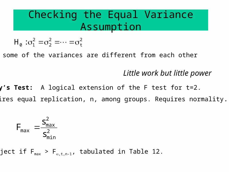
Checking the Equal Variance Assumption

2t

22

210 :H

Hartley’s Test: A logical extension of the F test for t=2.

2min

2max

max s

sF

Reject if Fmax > F,t,n-1, tabulated in Table 12.

HA: some of the variances are different from each other

Little work but little power

Requires equal replication, n, among groups. Requires normality.

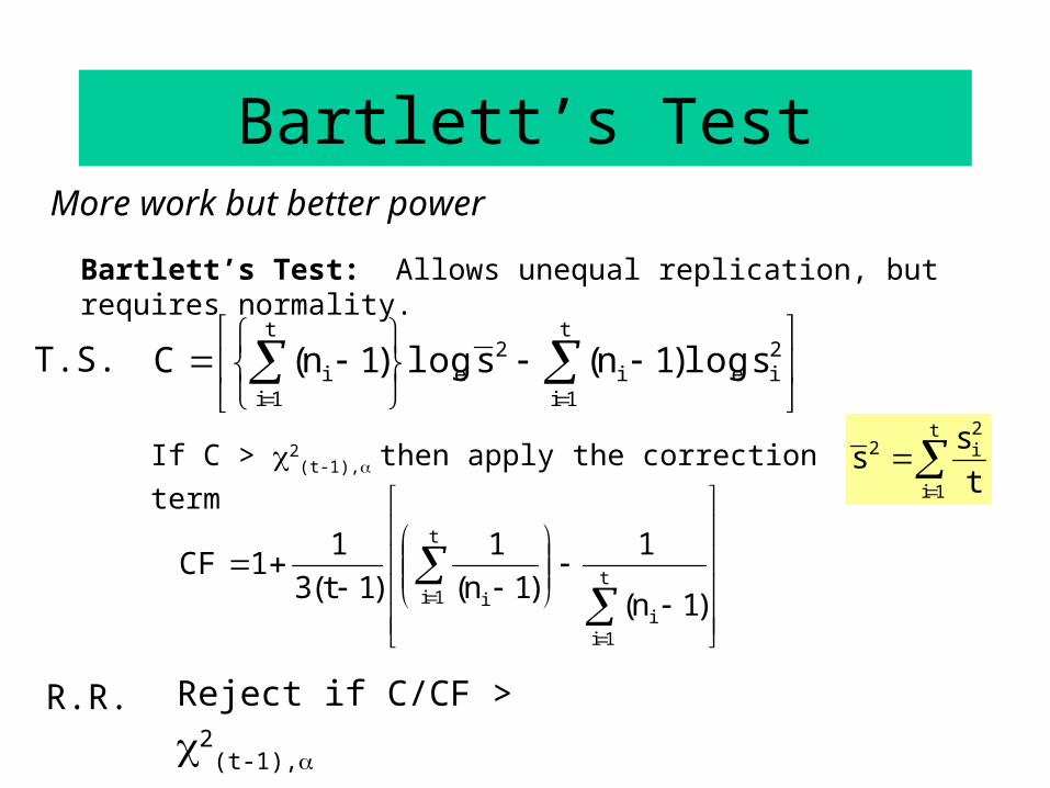
Bartlett’s Test

Bartlett’s Test: Allows unequal replication, but requires normality.

t

1i

2iei

2e

t

1ii slog)1n(slog)1n(C

t

1i

2i2

t

ssIf C > 2

(t-1),then apply the correction term

t

1ii

t

1i i )1n(

1

)1n(

1

)1t(3

11CF

Reject if C/CF > 2(t-1),

More work but better power

T.S.

R.R.

Levene’s Test

t

iTiij

n

ji

i

t

ii

tnzzn

tzznL

i

1

2

1

2

1

)/()(

)1/()(

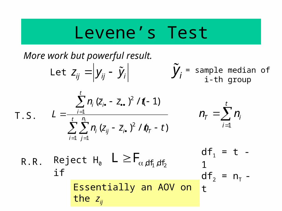
More work but powerful result.

T.S.

Let ij ij iz y y iy = sample median of i-th group

R.R. Reject H0 if 1 2,df ,dfL F df1 = t -1df2 = nT - t

Essentially an AOV on the zij

t

iiT nn

1

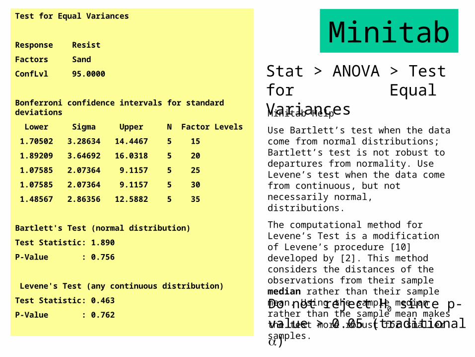
MinitabTest for Equal Variances

Response Resist

Factors Sand

ConfLvl 95.0000

Bonferroni confidence intervals for standard deviations

Lower Sigma Upper N Factor Levels

1.70502 3.28634 14.4467 5 15

1.89209 3.64692 16.0318 5 20

1.07585 2.07364 9.1157 5 25

1.07585 2.07364 9.1157 5 30

1.48567 2.86356 12.5882 5 35

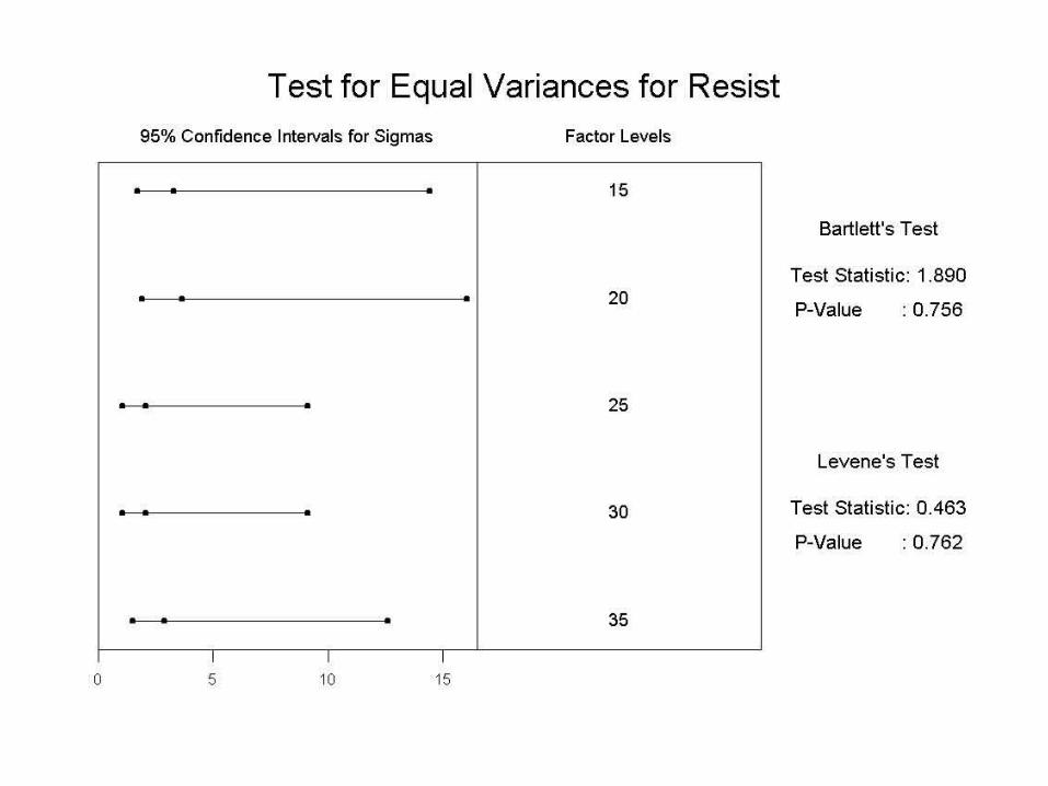
Bartlett's Test (normal distribution)

Test Statistic: 1.890

P-Value : 0.756

Levene's Test (any continuous distribution)

Test Statistic: 0.463

P-Value : 0.762Do not reject H0 since p-value >

0.05 (traditional )

Minitab Help

Use Bartlett’s test when the data come from normal distributions; Bartlett’s test is not robust to departures from normality. Use Levene’s test when the data come from continuous, but not necessarily normal, distributions.

The computational method for Levene’s Test is a modification of Levene’s procedure [10] developed by [2]. This method considers the distances of the observations from their sample median rather than their sample mean. Using the sample median rather than the sample mean makes the test more robust for smaller samples.

Stat > ANOVA > Test for Equal Variances

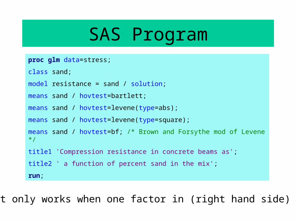
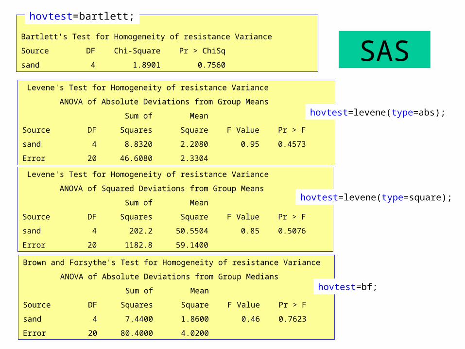
SAS Programproc glm data=stress;

class sand;

model resistance = sand / solution;

means sand / hovtest=bartlett;

means sand / hovtest=levene(type=abs);

means sand / hovtest=levene(type=square);

means sand / hovtest=bf; /* Brown and Forsythe mod of Levene */

title1 'Compression resistance in concrete beams as';

title2 ' a function of percent sand in the mix';

run;

Hovtest only works when one factor in (right hand side) model.

SASBartlett's Test for Homogeneity of resistance Variance

Source DF Chi-Square Pr > ChiSq

sand 4 1.8901 0.7560

Levene's Test for Homogeneity of resistance Variance

ANOVA of Absolute Deviations from Group Means

Sum of Mean

Source DF Squares Square F Value Pr > F

sand 4 8.8320 2.2080 0.95 0.4573

Error 20 46.6080 2.3304

Levene's Test for Homogeneity of resistance Variance

ANOVA of Squared Deviations from Group Means

Sum of Mean

Source DF Squares Square F Value Pr > F

sand 4 202.2 50.5504 0.85 0.5076

Error 20 1182.8 59.1400

Brown and Forsythe's Test for Homogeneity of resistance Variance

ANOVA of Absolute Deviations from Group Medians

Sum of Mean

Source DF Squares Square F Value Pr > F

sand 4 7.4400 1.8600 0.46 0.7623

Error 20 80.4000 4.0200

hovtest=bf;

hovtest=bartlett;

hovtest=levene(type=abs);

hovtest=levene(type=square);

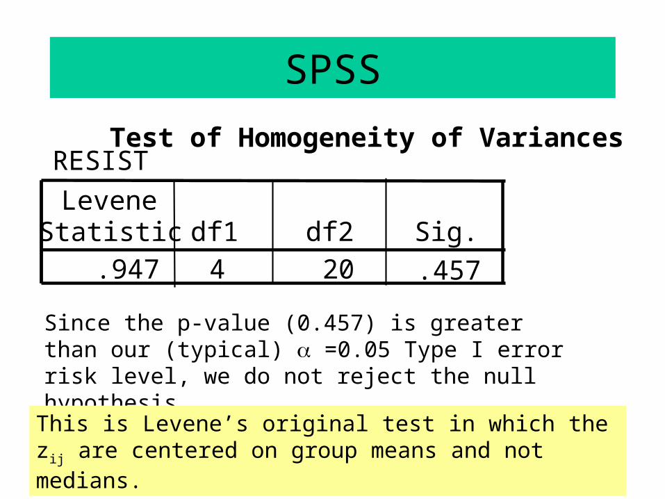
SPSS

Test of Homogeneity of VariancesRESIST

.947 4 20 .457

LeveneStatistic df1 df2 Sig.

Since the p-value (0.457) is greater than our (typical) =0.05 Type I error risk level, we do not reject the null hypothesis.

This is Levene’s original test in which the zij are centered on group means and not medians.

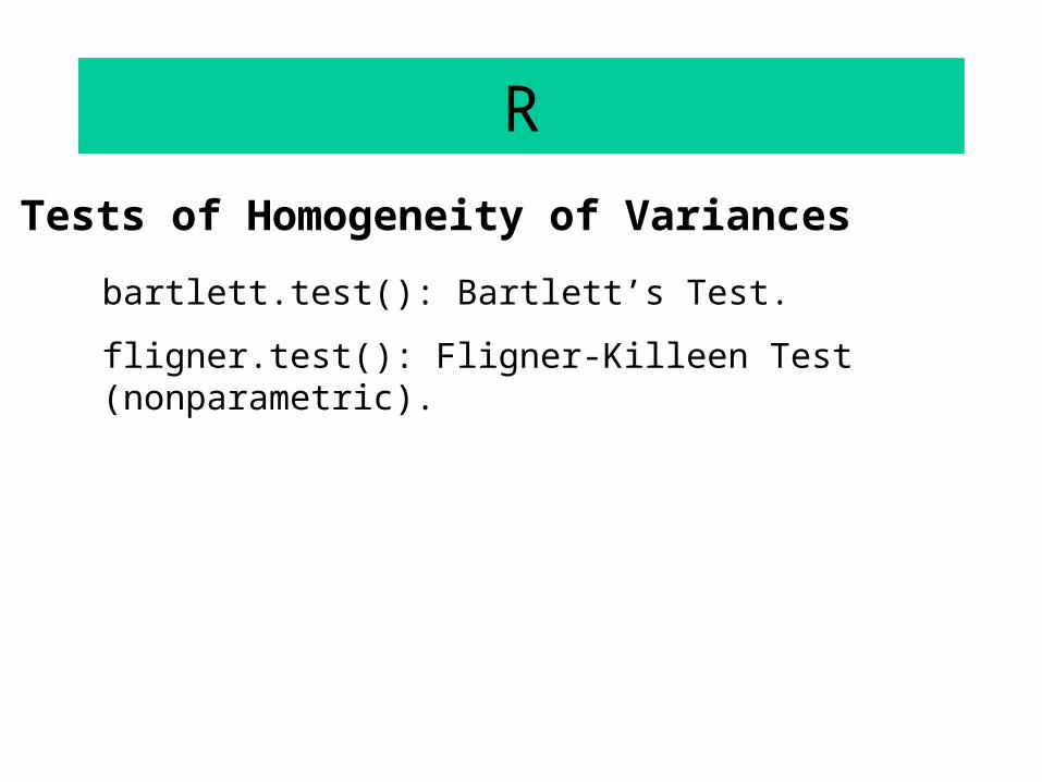
R

Tests of Homogeneity of Variances

bartlett.test(): Bartlett’s Test.

fligner.test(): Fligner-Killeen Test (nonparametric).

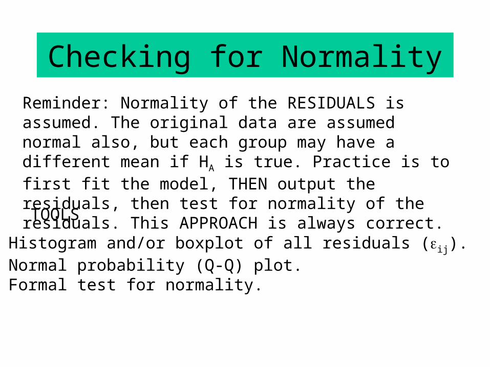
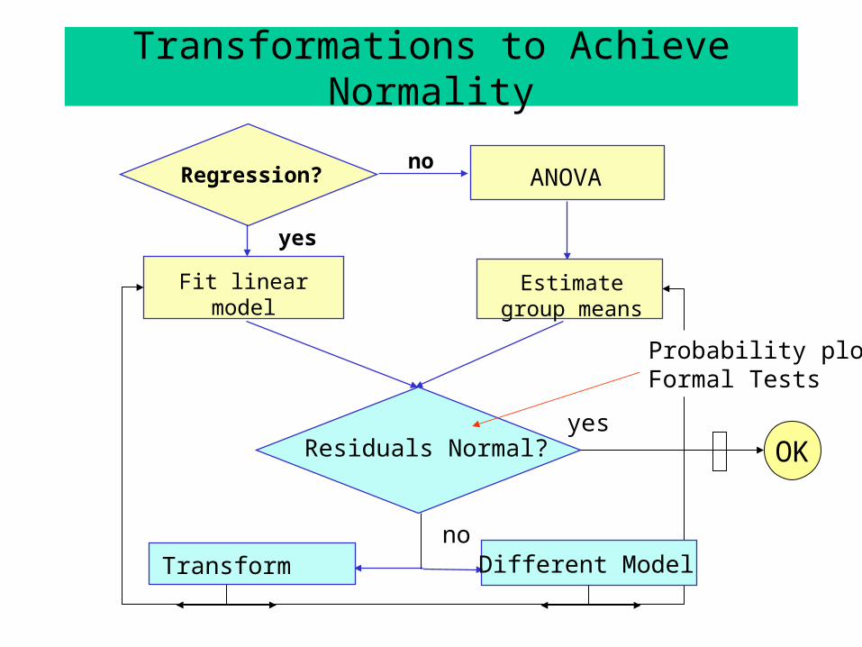
Checking for Normality

TOOLS

1. Histogram and/or boxplot of all residuals (ij).2. Normal probability (Q-Q) plot.3. Formal test for normality.

Reminder: Normality of the RESIDUALS is assumed. The original data are assumed normal also, but each group may have a different mean if HA is true. Practice is to first fit the model, THEN output the residuals, then test for normality of the residuals. This APPROACH is always correct.

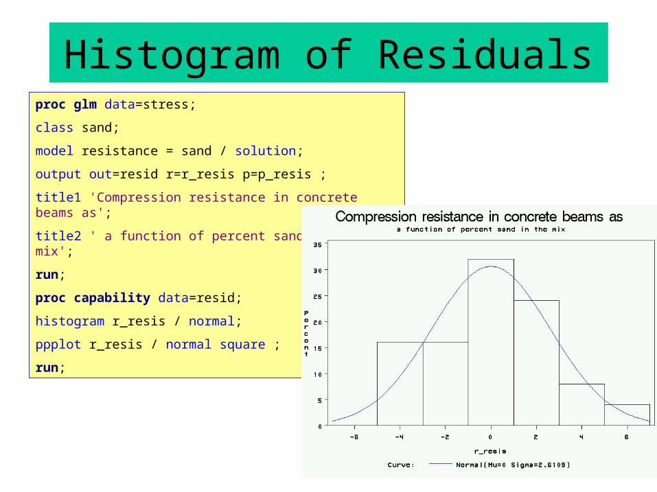
Histogram of Residualsproc glm data=stress;

class sand;

model resistance = sand / solution;

output out=resid r=r_resis p=p_resis ;

title1 'Compression resistance in concrete beams as';

title2 ' a function of percent sand in the mix';

run;

proc capability data=resid;

histogram r_resis / normal;

ppplot r_resis / normal square ;

run;

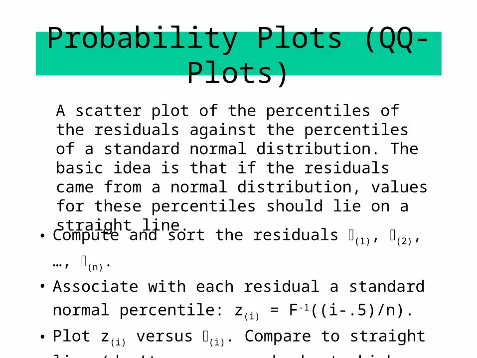
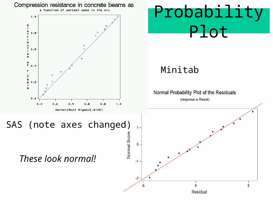
Probability Plots (QQ-Plots)

A scatter plot of the percentiles of the residuals against the percentiles of a standard normal distribution. The basic idea is that if the residuals came from a normal distribution, values for these percentiles should lie on a straight line.

• Compute and sort the residuals (1), (2),…, (n).

• Associate with each residual a standard normal

percentile: z(i) = F-1((i-.5)/n).

• Plot z(i) versus (i). Compare to straight line (don’t care

so much about which line).

SoftwarePercentile Residual Normal Percentile

0.02 -4.4 -2.05370.06 -3.8 -1.55480.10 -3.6 -1.28160.14 -3.4 -1.08030.18 -2.6 -0.91540.22 -2.6 -0.77220.26 -2.6 -0.64330.30 -1.6 -0.52440.34 -0.8 -0.41250.38 -0.6 -0.30550.42 0.2 -0.20190.46 0.2 -0.10040.50 0.4 0.00000.54 0.4 0.10040.58 0.4 0.20190.62 0.4 0.30550.66 1.4 0.41250.70 1.4 0.52440.74 1.4 0.64330.78 1.6 0.77220.82 2.4 0.91540.86 2.6 1.08030.90 3.6 1.28160.94 4.2 1.55480.98 5.4 2.0537

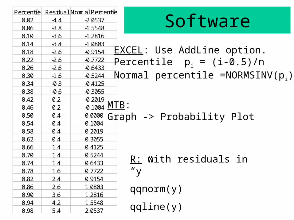
EXCEL: Use AddLine option.Percentile pi = (i-0.5)/nNormal percentile =NORMSINV(pi)

R: with residuals in “y”

qqnorm(y)

qqline(y)

MTB: Graph -> Probability Plot

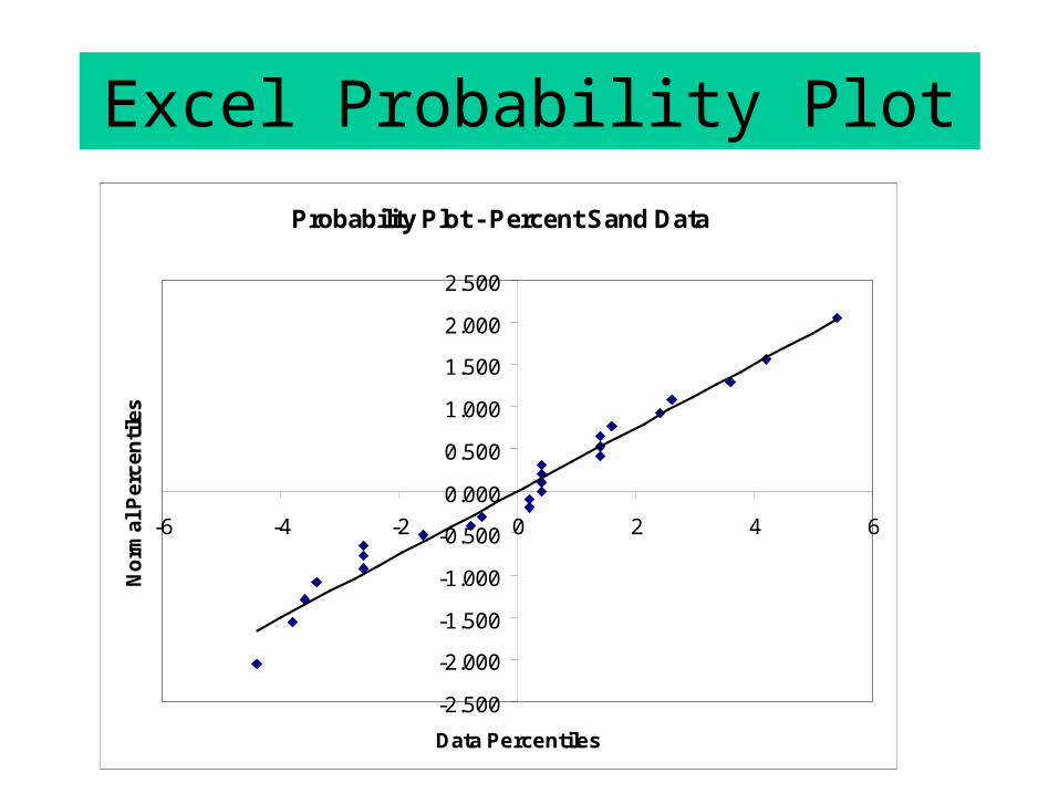
Excel Probability Plot

Probability Plot - Percent Sand Data

-2.500

-2.000

-1.500

-1.000

-0.500

0.000

0.500

1.000

1.500

2.000

2.500

-6 -4 -2 0 2 4 6

Data Percentiles

No

rmal

Per

cen

tile

s

Probability Plot

SAS (note axes changed)

Minitab

These look normal!

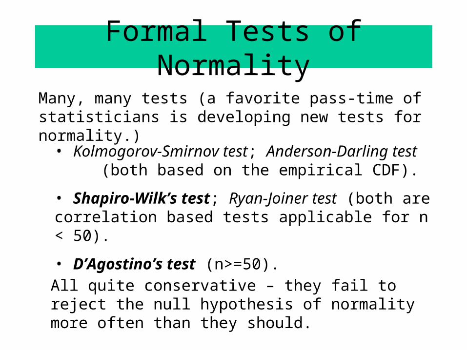
Formal Tests of Normality

• Kolmogorov-Smirnov test; Anderson-Darling test (both based on the empirical CDF).

• Shapiro-Wilk’s test; Ryan-Joiner test (both are correlation based tests applicable for n < 50).

• D’Agostino’s test (n>=50).

Many, many tests (a favorite pass-time of statisticians is developing new tests for normality.)

All quite conservative – they fail to reject the null hypothesis of normality more often than they should.

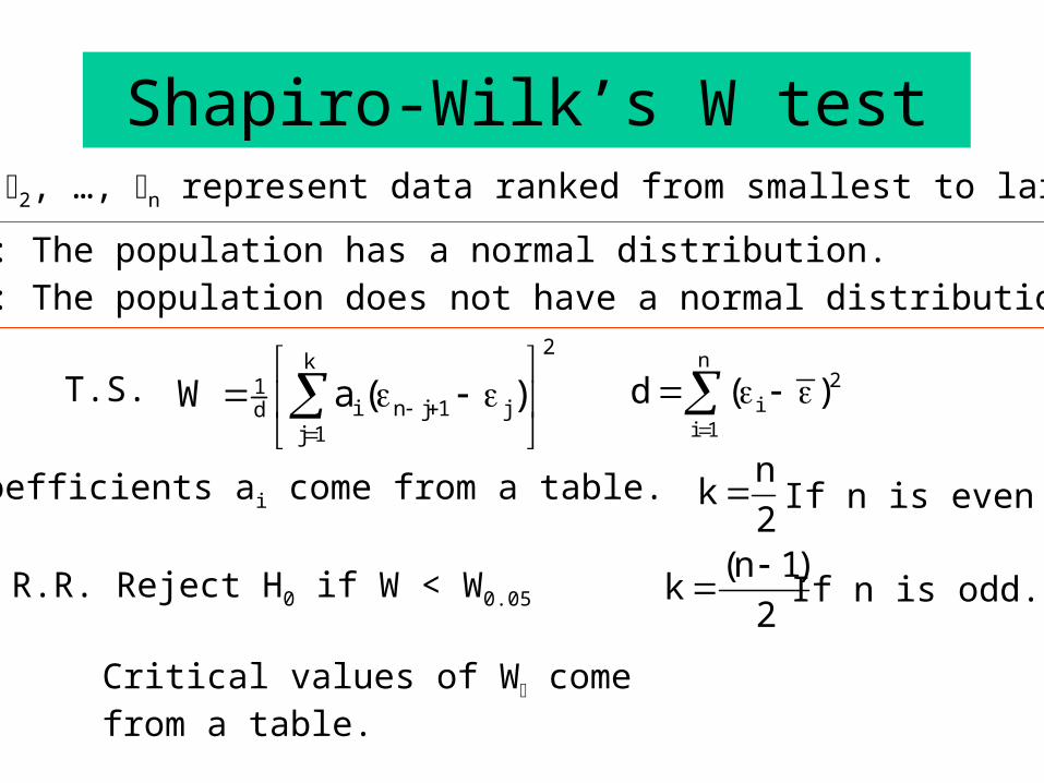
Shapiro-Wilk’s W test

2k

1i n j 1 jd

j 1

W a ( )

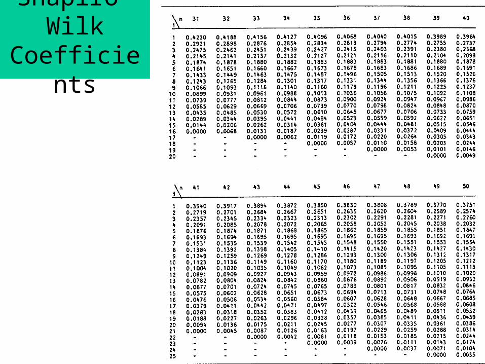
1, 2, …, n represent data ranked from smallest to largest.

H0: The population has a normal distribution.HA: The population does not have a normal distribution.

T.S.n

2i

i 1

d ( )

nk

2(n 1)

k2

If n is even

If n is odd.R.R. Reject H0 if W < W0.05

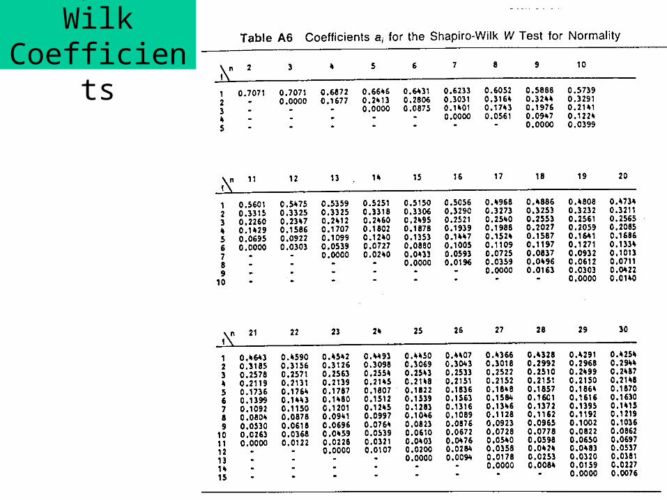
Coefficients ai come from a table.

Critical values of W come from a table.

Shapiro-Wilk Coefficients

Shapiro-Wilk Coefficients

Shapiro-Wilk W Table

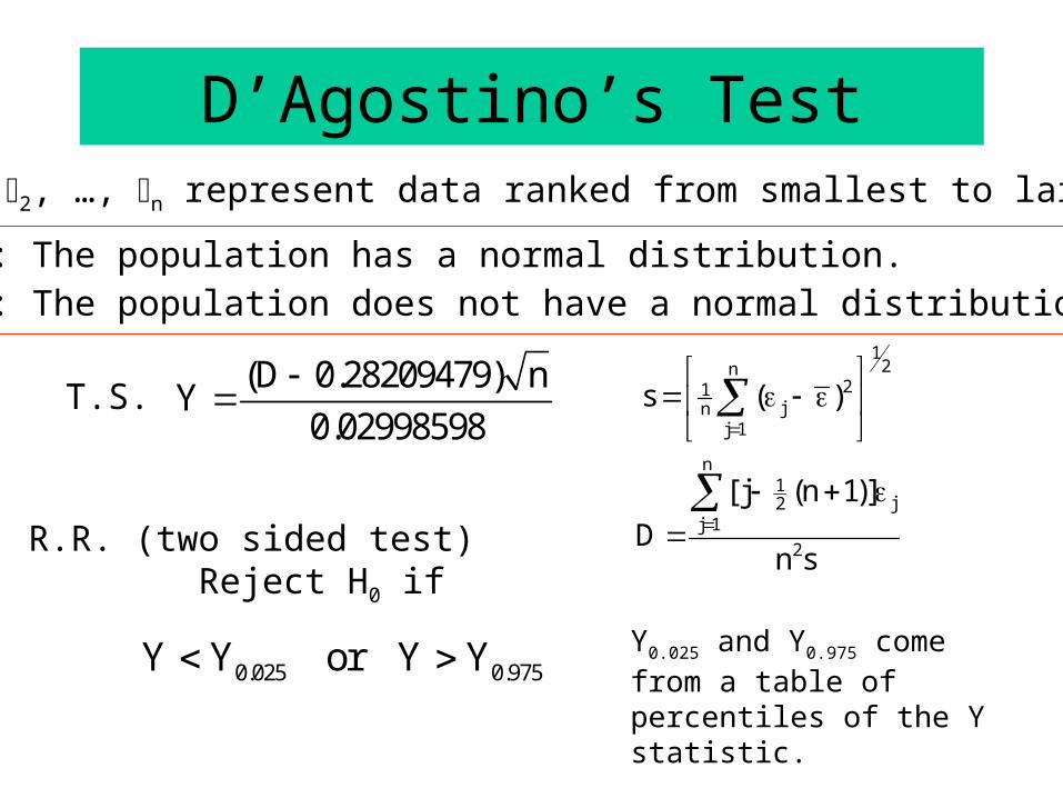
D’Agostino’s Test

(D 0.28209479) nY

0.02998598

12n

21jn

j 1

n1

j2j 1

2

s ( )

[ j (n 1)]

Dn s

1, 2, …, n represent data ranked from smallest to largest.

H0: The population has a normal distribution.HA: The population does not have a normal distribution.

T.S.

R.R. (two sided test) Reject H0 if

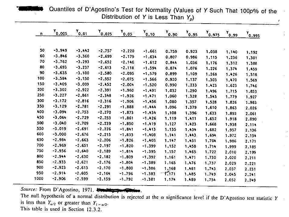
0.025 0.975Y Y or Y Y Y0.025 and Y0.975 come from a table of percentiles of the Y statistic.

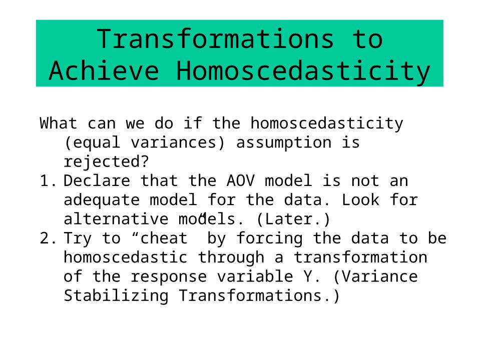
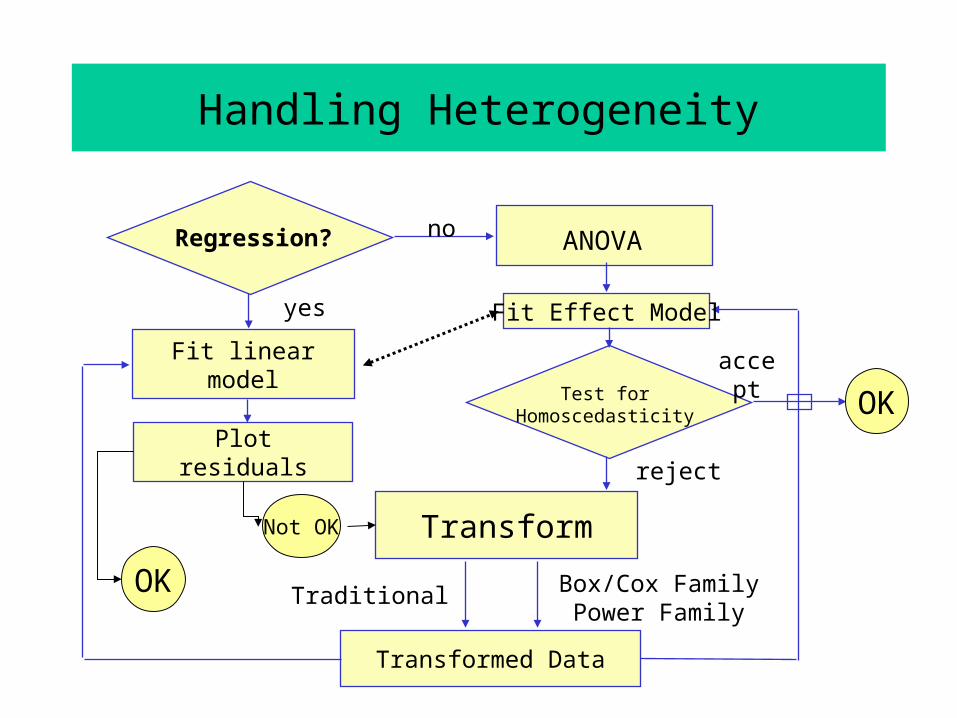
Transformations to Achieve Homoscedasticity

What can we do if the homoscedasticity (equal variances) assumption is rejected?

1. Declare that the AOV model is not an adequate model for the data. Look for alternative models. (Later.)

2. Try to “cheat” by forcing the data to be homoscedastic through a transformation of the response variable Y. (Variance Stabilizing Transformations.)

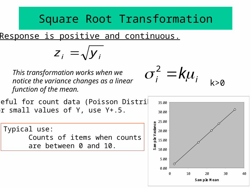
ii yz

i ik2 This transformation works when we notice the variance changes as a linear function of the mean.

• Useful for count data (Poisson Distributed).• For small values of Y, use Y+.5.

Typical use: Counts of items when countsare between 0 and 10.

Square Root Transformation

k>0

Response is positive and continuous.

0.00

5.00

10.00

15.00

20.00

25.00

30.00

35.00

0 10 20 30 40

Sample Mean

Sam

ple

Var

ian

ce

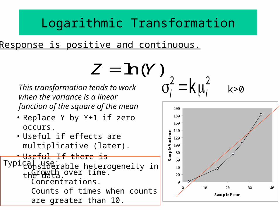
This transformation tends to work when the variance is a linear function of the square of the mean

• Replace Y by Y+1 if zero occurs.• Useful if effects are multiplicative (later).• Useful If there is considerable

heterogeneity in the data.

Z Yln( )2 2ki i

Typical use: Growth over time.Concentrations.Counts of times when countsare greater than 10.

Logarithmic Transformation

k>0

Response is positive and continuous.

0

20

40

60

80

100

120

140

160

180

200

0 10 20 30 40

Sample Mean

Sam

ple

Var

ian

ce

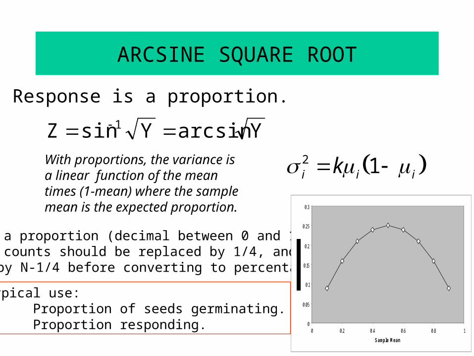
With proportions, the variance is a linear function of the mean times (1-mean) where the sample mean is the expected proportion.

• Y is a proportion (decimal between 0 and 1).• Zero counts should be replaced by 1/4, and N by N-1/4 before converting to percentages

YarcsinYsinZ 1

i i ik2 1

Response is a proportion.

Typical use: Proportion of seeds germinating.Proportion responding.

ARCSINE SQUARE ROOT

0

0.05

0.1

0.15

0.2

0.25

0.3

0 0.2 0.4 0.6 0.8 1

Sample Mean

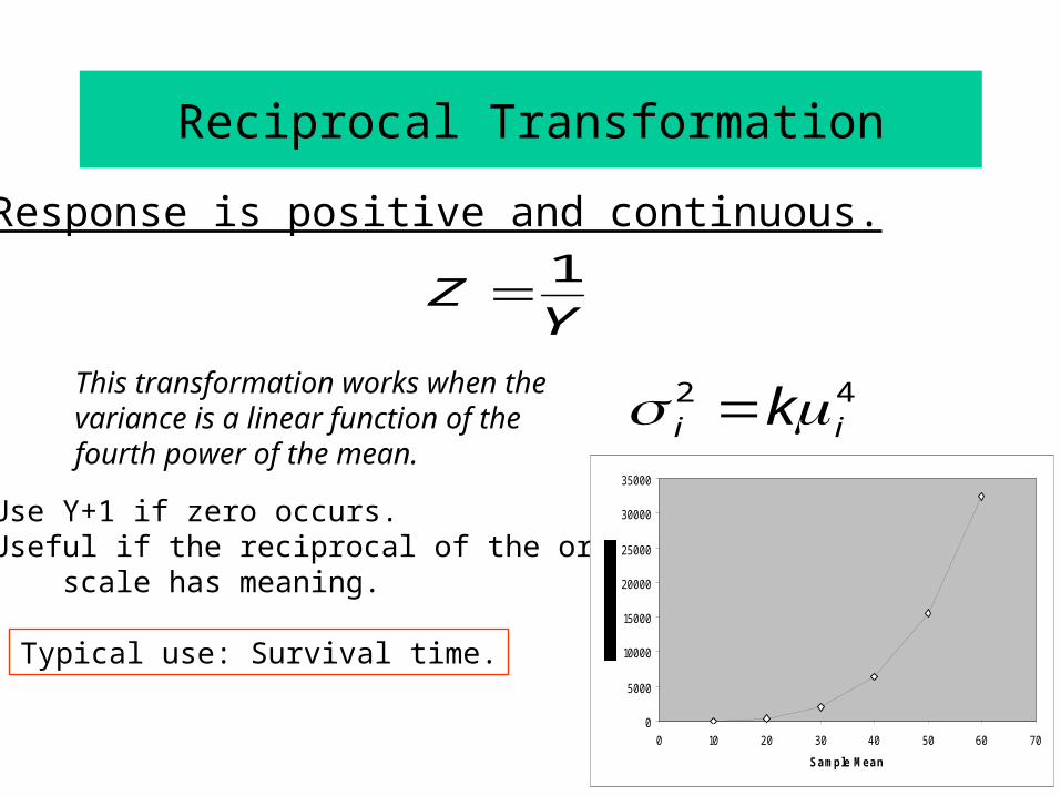
Response is positive and continuous.

This transformation works when the variance is a linear function of the fourth power of the mean.

• Use Y+1 if zero occurs.• Useful if the reciprocal of the original

scale has meaning.

ZY

1

i ik2 4

Typical use: Survival time.

Reciprocal Transformation

0

5000

10000

15000

20000

25000

30000

35000

0 10 20 30 40 50 60 70

Sample Mean

ii k2

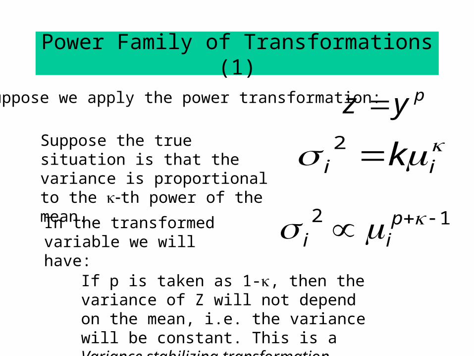
Suppose we apply the power transformation: pyz Suppose the true situation is that the variance is proportional to the th power of the mean.

If p is taken as 1-, then the variance of Z will not depend on the mean, i.e. the variance will be constant. This is a Variance stabilizing transformation.

Power Family of Transformations (1)

In the transformed variable we will have:

12 pii

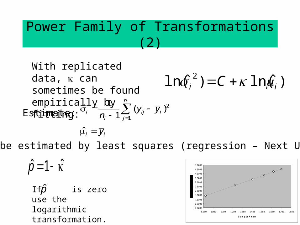
With replicated data, can sometimes be found empirically by fitting:

Estimate:2

1

1ˆ ( )

1

ˆ

in

i ij iji

i i

y yn

y

can be estimated by least squares (regression – Next Unit).

ˆˆ 1p If is zero use the logarithmic transformation.

p̂

Power Family of Transformations (2)

0.0000

0.5000

1.0000

1.5000

2.0000

2.5000

3.0000

3.5000

4.0000

4.5000

5.0000

0.980 1.080 1.180 1.280 1.380 1.480 1.580 1.680 1.780 1.880

Sample Mean

)ˆln()ˆln( 2ii C

n

ii

i

i

i

yn

y

yz

1

1

ln1

exp

0ln

01

suggestedtransformation

geometric mean of the original data.

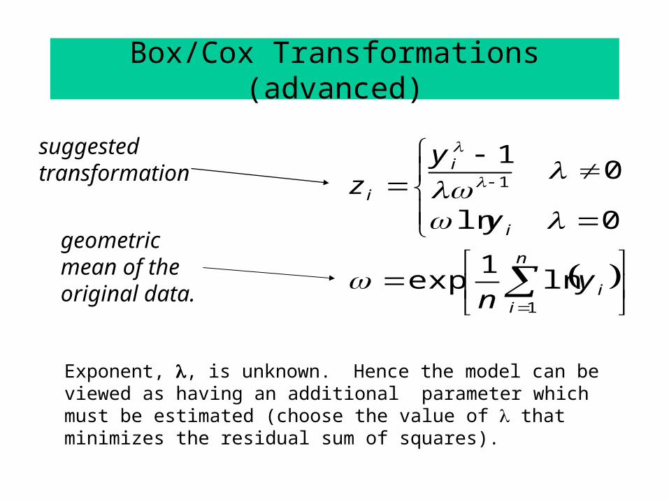
Exponent, , is unknown. Hence the model can be viewed as having an additional parameter which must be estimated (choose the value of that minimizes the residual sum of squares).

Box/Cox Transformations (advanced)

Regression? ANOVAno

yes

Test forHomoscedasticity

reject

accept

Transform

Transformed Data

Box/Cox FamilyPower Family

Traditional

Fit linearmodel

Plotresiduals

Fit Effect Model

Handling Heterogeneity

Not OK

OK

OK

Regression? ANOVAno

yes

Fit linearmodel

Estimategroup means

Residuals Normal?

no

yes

Transform Different Model

Probability plotFormal Tests

Transformations to Achieve Normality

OK