AP237/Bio251 Problem Set 3 Solutions Written/compiled by: Benjamin Good and Anita Kulkarni March 7, 2021 Problem 1: Heuristics for recessive mutations Part A The short-time approximation of our SDE is f (Δt)= f (0) + sf 2 (0)Δt + r f (0)Δt 2N Z This approximation is valid up to logarithmic (order-of-magnitude) precision on a timescale ∼ Δt reset ; to find the frequency boundary between drift-dominated and selection-dominated regimes, check whether deterministic or stochastic forces are dominant on this timescale (look for self-consistency), similar to what was done in class for the haploid case. • If deterministic forces are dominant, f (0) ∼|f (Δt reset ) - f (0)|∼|s|f 2 (0)Δt reset = ⇒ Δt reset ∼ 1 f |s| On this timescale, the contribution from drift is s f 2N 1 f |s| = s 1 2N |s| Dropping constant factors, we get that |Δf drift ||Δf sel |∼ f when f 1 p N |s| • Similarly, perform a self-consistency check under the assumption that stochastic forces are dominant. Under this assumption, f ∼|Δf drift |∼ r f Δt reset 2N = ⇒ Δt reset ∼ 2Nf On this timescale, the contribution from selection is 2Nsf 3 , and for this to be f , we need f 1 √ 2N|s| . Thus, |Δf sel ||Δf drift |∼ f when f 1 p N |s| and we have self-consistency. Drift dominates below f ∼ 1/ p N |s|, and selection dominates above f ∼ 1/ p N |s|. In order for selection to be effective in at least some part of frequency space, we need the frequency boundary to be 1; rearranging, we find that N |s| 1. 1
Transcript
AP237/Bio251 Problem Set 3 Solutions
Written/compiled by: Benjamin Good and Anita Kulkarni
March 7, 2021
Problem 1: Heuristics for recessive mutations
Part A
The short-time approximation of our SDE is
f(∆t) = f(0) + sf2(0)∆t+
√f(0)∆t
2NZ
This approximation is valid up to logarithmic (order-of-magnitude) precision on a timescale ∼ ∆treset;to find the frequency boundary between drift-dominated and selection-dominated regimes, check whetherdeterministic or stochastic forces are dominant on this timescale (look for self-consistency), similar to whatwas done in class for the haploid case.
On this timescale, the contribution from drift is√f
2N
1
f |s|=
√1
2N |s|
Dropping constant factors, we get that |∆fdrift| � |∆fsel| ∼ f when
f � 1√N |s|
• Similarly, perform a self-consistency check under the assumption that stochastic forces are dominant.Under this assumption,
f ∼ |∆fdrift| ∼√f∆treset
2N=⇒ ∆treset ∼ 2Nf
On this timescale, the contribution from selection is 2Nsf3, and for this to be � f , we need f �1√
2N |s|. Thus, |∆fsel| � |∆fdrift| ∼ f when
f � 1√N |s|
and we have self-consistency.
Drift dominates below f ∼ 1/√N |s|, and selection dominates above f ∼ 1/
√N |s|. In order for selection to
be effective in at least some part of frequency space, we need the frequency boundary to be� 1; rearranging,we find that N |s| � 1.
1
Part B
The following heuristic result derived in class is not haploid-specific (i.e. the derivation did not utilize anyparticular properties of the haploid SDE): a mutant with initial size f0 drifts to final (boundary) size f withprobability f0/f on a timescale of ∼ Nf generations. Plugging in our results from part a, assuming s� 1,we get that a mutant with initial size ∼ 1
N drifts to boundary size ∼ 1√Ns
with probability ∼√
sN on a
timescale of ∼√
Ns generations.
Since the mutation is strongly beneficial, once its frequency reaches f∗ ∼ 1/√Ns, it is guaranteed to fix
deterministically. How long will this part take? To get a rough estimate, solve the deterministic equation(in the low-frequency limit since this is more tractable) with f(0) = f∗:
∂f
∂t= sf2 =⇒ f(t) =
f∗
1− f∗st
From this, we see that f(t) = 12 when
t1/2 =1
s(
1
f∗− 2) =
1
s(√Ns− 2) ∼
√N
s
Both the time to the drift boundary and subsequent deterministic time to frequency 0.5 are of order√N/s,
so in general the time to fixation is of order√N/s (with probability ∼
√s/N , as we saw before). When
Ns� 1, the fixation probability is smaller than that of the haploid case, and the fixation time is larger.
Part C
The results from part b for below the drift barrier still apply for strongly deleterious mutations (a stronglydeleterious mutant will not grow much past the drift barrier): a strongly deleterious mutant with initial size
∼ 1N drifts to final size ∼ 1√
N |s|with probability ∼
√|s|N on a timescale of ∼
√N|s| generations. Plugging in
numbers, we get that a recessive mutation with fitness effect s ≈ −1 in a population of N = 106 individualswill typically grow to maximum frequency ∼ 10−3 and exist for ∼ 103 generations.
Problem 2: The molecular diversity of adaptive convergence
Part A
We calculate dN/dS by computing (# of observed nonsynonymous mutations/# of possible nonsynonymousmutations, from problem set 1)/(# of observed synonymous mutations/# of possible synonymous muta-tions, from problem set 1). The numbers of possible mutations from the posted problem set 1 solutionsas of February 24, 2021 (3,059,233 possible synonymous mutations, 404,289 possible nonsense mutations,and 8,587,451 possible missense mutations) yield a dN/dS for missense mutations of 4.81 and dN/dS fornonsense mutations of 4.04. Other reasonable choices of numbers may yield ratios near roughly 4-5 and 3-4,respectively. Either way, these are quite far from 1 and we can confidently say that mutations in both classesare positively selected.
2
Part B
Figure 1: Number of sites mutated m or more times across all n = 114 replicates, plotted as a function ofm.
If all 789 mutations were distributed evenly across the sites in the E. coli genome, then we would expectthe number of mutations on each site to be roughly Poisson distributed. Given that the E. coli genome isL = 4, 629, 812 bp long, this distribution would have a mean of λ = 789/4, 629, 812 ≈ 1.7 × 10⁻⁴. Thus,under our assumptions, the number of sites expected to have ≥ m mutations would be
L×
(1−
m−1∑k=0
λke−λ
k!
)
Plugging in numbers, ≈ 788.9 sites would be expected to have ≥ 1 mutation, and ≈ 0.067 sites wouldbe expected to have ≥ 2 mutations. Since 53 � 0.067 sites had ≥ 2 mutations, we can safely say thatsites with two or more mutations are likely to have experienced beneficial selection. Using this criterion,192/789 ≈ 24.3% of observed mutation events are likely to have come from a beneficially selected site.
Part C
Figure 2: Number of genes mutated m or more times across all n = 114 replicates, plotted as a function ofm.
Repeat a similar analysis as in part b. When counting synonymous, missense, nonsense, and within-geneindel mutations, 833 different genes were found to have mutated. Given that there are L = 4, 217 genes in
3
the E. coli genome (and making the simplifying assumption that each gene is equally likely to mutate, i.e.is equally long), our Poisson distribution has λ = 833/4217 ≈ 0.198. This yields ≈ 755.9 genes expected tohave ≥ 1 mutation, ≈ 72.2 genes expected to have ≥ 2 mutations, and ≈ 4.67 genes expected to have ≥ 3mutations. The observed values are 291, 69, and 46, respectively, and since 46� 4.67, we can safely say thatgenes with three or more mutations are likely to have experienced beneficial selection. Under this criterion,565/833 ≈ 67.8% of observed mutation events are likely to have come from a beneficially selected gene.
Part D
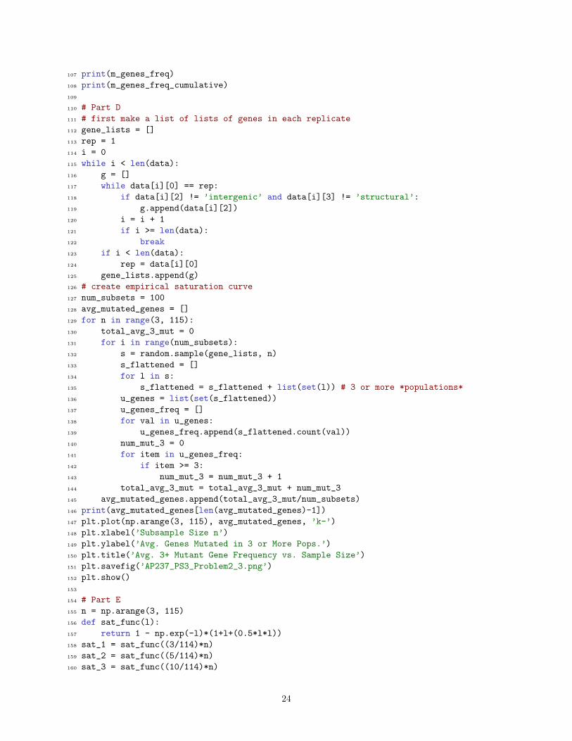
Figure 3: Empirical saturation curve, or average (over 100 trials) number of genes mutated (point or indelmutations within genes) in 3 or more randomly sampled populations of sample size n = 3, . . . , 114.
The curve slows down but does not appear to fully saturate by n = 114.
Part E
The probability (exact, based on the binomial distribution) of observing m mutations in gene i (with prob-ability pi of being mutated in a given population) across ≥ 3 populations in an experiment with n totalpopulations is:
1− (1− pi)n − npi(1− pi)n−1 −n(n− 1)
2p2i (1− pi)n−2
Another decent approximation based on the Poisson distribution is
1− e−npi(
1 + npi +n2p2i
2
)Three theoretical saturation curves (the above probability plotted for different values of n) for pi = 3
114 ,5
114 ,10114
are given below.
4
Figure 4: Theoretical saturation curves as described in the text. The blue curve corresponds to pi = 3114 ,
the orange curve corresponds to pi = 5114 , and the green curve corresponds to pi = 10
114 .
For pi = 3114 , approximately 57.7% of beneficial genes will be detected in an experiment with n = 114
replicates, for pi = 5114 , approximately 87.5% will be detected, and for pi = 10
114 , approximately 99.7% will bedetected (these were calculated using the Poisson approximation). Our empirical saturation curve roughlyresembles the curve for pi = 5
114 (except at small sample sizes, of course different genes could have differentpi’s). 45 beneficial genes were detected for n = 114, and if these correspond to 87.5% of total beneficialgenes, then ≈ 50 genes are likely to be beneficial in this environment.
Part F
We find that 43 total replicates have a (non-structural) mutation in rho, 29 total replicates have a mutationin iclR, and 20 replicates have mutations in both rho and iclR. By chance alone, we would expect
114× 43
114× 29
114≈ 11
replicates to have mutations in both genes, which is only half as big as the observed value. Statisticalsignificance can be assessed using Fisher’s exact test — i.e., the probability that we observe 20 or more lineswith both mutations by chance is given by
P =
29∑k=20
(43k
)(114−4329−k
)(11429
) 10−4 (1)
This suggests that iclR mutations do tend to be more beneficial on a background of rho than without.However, 9 replicates still have a mutation in iclR alone, which is still significantly beneficial under ouroriginal 3-replicate threshold, suggesting that iclR are not exclusively beneficial in the presence of ρ.
Problem 3: Measuring the DFE for de novo beneficial mutations,Part I
We’ll make use of the fact that this serial dilution experiment is equivalent to a diffusion model with aneffective population size Ne ∼ N0∆. We’ll then consider each of the four criteria in reverse order:
1. Each barcoded lineage will start at a characteristic frequency f0∼1/B. Genetic drift will require atime of order ∼Nef0 = Ne/B generations to substantially perturb the frequency of these lineages, sowe need to make sure that the total experimental duration is less than this time:
T .NeB
(2)
5
2. Conversely, beneficial mutations will require ∼1/sb generations to substantially change the lineagefrequency, so we want to make sure that the total duration is longer than this time. Combining withthe condition above, this yields
1
sb. T .
NeB
(3)
3. Each barcoded lineage will produce ∼(Ne/B)UbsbT successful beneficial mutations over the courseof the experiment. We’ll want this number to be � 1 so there is a small probablity of producingtwo beneficial mutations in the same lineage. Let’s pick 0.01 for concretness (i.e., 99% of putativelyadaptive barcodes will contain a single beneficial mutation). This leads to a condition,
NeBUbsbT . 0.01 (4)
4. Finally, we want to make sure we have & 1000 lineages with at least one mutation. If each of the Blineages produces a beneficial mutation with probability ∼(Ne/B)UbsbT , this requires that
NeUbsbT & 1000 (5)
Now to plug in some numbers. If sb ∼ 10−2, then the second condition requires that
T & 100 (6)
It’s always easier if we run a shorter experiment, so let’s see how far we can get with T∼100. If Ub∼10−5,then the last condition requires that
Ne & 108 (7)
Meanwhile, the 3rd and 4th conditions together require that
B & 105 (8)
By choosing Ne = 108 and B = 105, we see that the first condition is satisfied. All four conditions are thensatsified. To implement this in a serial dilution experiment, we’d want to make sure that s∆t� 1. This canbe achived by taking ∆t = 10 and a bottleneck size of N0 = 107, and running the experiment for T/∆t = 10days.
Finally, the sequencing depth must be chosen to be sufficiently high that we can resolve the relevant selectionpressures. For a barcode at frequency ∼1/B, the relative error in our frequency estimate will be of order∼√B/D. If we want this to be no more than 10% at each timepoint, we will require
D & 100B (9)
or about ∼107 reads per timepoint. All 10 timepoints for a single replicate could therefore fit on a singlelane of Illumina sequencing (∼ 108 total reads).
6
7
8
9
10
11
12
13
14
15
16
17
18
19
20
21
Sample code for Problem Set 3
1 # Code for Problem 2 of Problem Set 3
2
3 # -*- coding: utf-8 -*-
4 """
5 Created on Mon Feb 17 00:47:03 2020
6
7 @author: Anita Kulkarni
8 """
9
10 import numpy as np
11 import random
12 import matplotlib.pyplot as plt
13
14 f = open("./data_files/problem_set_data/tenaillon_etal_2012_mutations.txt","r")
15 raw_data = f.readlines()
16 del(raw_data[0])
17
18 data = []
19 for i in range(len(raw_data)):
20 l = raw_data[i].split(", ")
21 # get rid of last two columns (allele, functional module)
22 del(l[len(l)-1])
23 del(l[len(l)-1])
24 l[0] = int(l[0][4:len(l[0])]) # lineage number
25 l[1] = int(l[1]) # mutation location
26 l = tuple(l)
27 data.append(l)
28
29 # Part A
30 n_synonymous = 0
31 n_missense = 0
32 n_nonsense = 0
33 for i in range(len(data)):
34 if data[i][3] == ’synonymous’:
35 n_synonymous = n_synonymous + 1
36 elif data[i][3] == ’missense’:
37 n_missense = n_missense + 1
38 elif data[i][3] == ’nonsense’:
39 n_nonsense = n_nonsense + 1
40 possible_synonymous = 3059233
41 possible_missense = 8587451
42 possible_nonsense = 404289
43 S = n_synonymous/possible_synonymous
44 N1 = n_missense/possible_missense
45 N2 = n_nonsense/possible_nonsense
46 print(N1/S)
47 print(N2/S)
48
49 # Part B
50 point_mutation_sites = []
51 for i in range(len(data)):
52 if data[i][3] == ’synonymous’ or data[i][3] == ’missense’ or data[i][3] == ’nonsense’ or data[i][3] == ’noncoding’: