APM 504: Continuous-time Markov Chainsjtaylor/teaching/Spring2015/APM504/... · APM 504:...

;

APM 504: Continuous-time Markov Chains

Jay TaylorSpring 2015

Jay Taylor (ASU) APM 504 Spring 2015 1 / 55

Outline

1 Definitions

2 Example: Jukes-Cantor Model

3 The Gillespie Algorithm

4 Kolmogorov Equations

5 Stationary Distributions

6 Poisson Processes


Definitions

We begin with a general definition that imposes no restrictions on E . As in thediscrete-time setting, the gist of the definition is that the past and the future areconditionally independent given the present.

Continuous-time Markov ProcessesA stochastic process X = (Xt ; t ≥ 0) with values in a set E is said to be acontinuous-time Markov process if for every sequence of times0 ≤ t1 < · · · < tn < tn+1 and every set of values x1, · · · , xn+1 ∈ E , we have

P (Xtn+1 ∈ A|Xtn = xn, · · · ,Xt1 = x1) = P (Xtn+1 ∈ A|Xtn = xn) ,

whenever A is a subset of E such that Xtn+1 ∈ A is an event. In this case, thefunction defined by

p(s, t; x ,A) = P(Xt ∈ A|Xs = x), t ≥ s ≥ 0

is called the transition function of X . If this function depends on s and t only throughthe difference t − s, then we say that X is time-homogeneous.


Definitions

Examples of continuous-time Markov processes encountered in biology include:

continuous-time Markov chains, e.g., nucleotide substitution models (JC69, HKY,GTR); the Moran model; Kingman’s coalescent; the Moran model

continuous-time branching processes

continuous-time random walks

Poisson processes

diffusion processes and the solutions to stochastic differential equations, e.g.,Brownian motion and the Ornstein-Uhlenbeck process

Levy processes, e.g., Levy flight


Definitions

Sample Paths

A continuous-time stochastic process X = (Xt : t ≥ 0) can be thought of in twodifferent ways.

On the one hand, X is simply a collection of random variables defined on the sameprobability space, Ω.

On the other hand, we can also think of X as a path- or function-valued randomvariable. In other words, given an outcome ω ∈ Ω, we will view X (ω) as a functionfrom [0,∞) into E defined by

X (ω)(t) ≡ Xt(ω) ∈ E .

The path traced out by X (ω) as t varies from 0 to ∞ is said to be a sample path of X .


Definitions

In these notes, we will mainly be concerned with time-homogeneous Markov processesthat take values in countable state spaces: E = 1, 2, · · · , n or E = 1, 2, · · · . As wewill see, these processes are jump processes.

Continuous-time Markov ChainsA stochastic process X = (Xt ; t ≥ 0) with values in a countable set E is said to be acontinuous-time Markov chain (CTMC) if there are functions

pij : [0,∞)→ [0, 1], i , j ∈ E

such that for every sequence of times 0 ≤ t1 < · · · < tn < tn+1 and every set of valuesx1, · · · , xn+1 ∈ E we have

P (Xtn+1 = xn+1|Xtn = xn, · · · ,Xt1 = x1) = P (Xtn+1 = xn+1|Xtn = xn)

= pxn,xn+1 (tn+1 − tn).

The functions pij(t) are said to be the transition functions of X .


Definitions

Transition Semigroups

If X = (Xt : t ≥ 0) is a continuous-time Markov chain, we can define an entire family oftransition matrices indexed by time. Specifically, for each t ≥ 0 and each pair ofelements i , j ∈ E , let

pij(t) = P(Xt = j |X0 = i)

be the transition function corresponding to transitions from state i to state j , and letP(t) be the matrix with entries pij(t). In particular, if E = 1, 2, · · · , n is finite, thenP(t) is the n × n matrix

P(t) =

p11(t) p12(t) · · · p1n(t)p21(t) p22(t) · · · p2n(t)

......

...pn1(t) pn2(t) · · · pnn(t)

.


Definitions

It can be shown that the family of transition matrices (P(t) : t ≥ 0) satisfies thefollowing properties:

For each t ≥ 0, P(t) is a stochastic matrix:∑j∈E

pij(t) = 1.

P(0) is the identity matrix: pii (0) = 1 and pij(0) = 0 if j 6= i .

For every s, t ≥ 0, the matrices P(s) and P(t) commute and

P(t + s) = P(t)P(s).

The third property is called the semigroup property and the family of matrices is saidto be a transition semigroup. When written in terms of coordinates, this property is

pij(s + t) =∑k∈E

pik(s)pkj(t)

which is just the continuous-time version of the Chapman-Kolmogorov equations.


Definitions

One consequence of the semigroup property is that for any t ≥ 0 and any n ≥ 1, we have

P(t) = P(t/n)n.

In fact, provided that the matrices P(t) depend continuously on t, it can be shown thatthere exists a unique matrix Q such that for every t ≥ 0

P(t) = eQt ≡∞∑n=0

1

n!tnQn.

This matrix is called the rate matrix (or the generator matrix, infinitesimal matrix, orQ-matrix) of the continuous-time Markov chain X . Rate matrices play a central role inthe description and analysis of continuous-time Markov chain and have a specialstructure which is described in the next theorem.


Definitions

Structure of the Q-matrixLet Q = (qij) be the rate matrix of a continuous-time Markov chain X with transitionsemigroup (P(t) : t ≥ 0). Then all of the row-sums of Q are equal to 0 and all of theoff-diagonal elements are non-negative:

qij ≥ 0 if j 6= i

qii = −∑j 6=i

qij ,

Furthermore, each transition probability pij(t) is a differentiable function of t and

qij = p′ij(0) = limt→0

pij(t)− pij(0)

t.

Remark: In matrix notation, these identities can be written as

Q = P ′(0) = limt→0

1

t

(P(t)− I

).


Definitions

This theorem explains why Q is called the rate matrix of the process X . Provided thatt > 0 is sufficiently small,

pij(t) = P (Xt = j |X0 = i) =

qij t + o(t) if j 6= i1 + qii t + o(t) if j = i ,

which shows that the probability that the process moves from its current state i toanother state j during a short period of time t is approximately proportional to theamount of time elapsed. In other words, qij is the rate at which transitions occur fromstate i to state j , while |qii | is the total rate at which the process jumps out of state i .


Definitions

Construction and Simulation of CTMC’s

Suppose that X = (Xt : t ≥ 0) is a CTMC with rate matrix Q and that the entries of Qare bounded, i.e., for some M <∞, |qij | < M for all i , j ∈ E . Our goal in this section isto show how we can simulate X . The construction will use the following objects:

A probability distribution ν on E which will be the initial distribution of the chain.

A collection of independent exponentially-distributed random variablesη

(n)ij ; n ≥ 0; i , j ∈ E , j 6= i

,

where η(n)ij has rate parameter qij . If qij = 0, we set η

(n)ij =∞.

For each n ≥ 1 and each i , j ∈ E , we will think of η(n)ij as the time when a random alarm

clock sounds its alarm.


Definitions

The process X is constructed recursively according to the following procedure:

Sample a state i0 ∈ E with probability νi0 and set X0 = i0; this is the initial stateof the chain.

Conditional on X0 = i0, let

τ1 ≡ minη

(0)i0,j

: j 6= i0

i1 ≡ arg minj

η

(0)i0,j

: j 6= i0,

i.e., the state i1 ∈ E is determined by the clock η(0)i0,i1

that is the first to ring.

Let J1 = τ1 and define X on the interval [0, J1] by setting

Xt =

i0 if t ∈ [0, J1)i1 if t = J1.

Interpretation: The process occupies state i0 up until the time of the first jump, J1, atwhich point it moves to state i1.


Definitions

In general,

Conditional on XJn = in, let

τn+1 ≡ minη

(n)in,j

: j 6= in

in+1 ≡ arg minj

η

(n)in,j

: j 6= in.

Let Jn+1 = Jn + τn+1, and define X on the interval [Jn, Jn+1] by setting

Xt =

in if t ∈ [Jn, Jn+1)in+1 if t = Jn+1.

Interpretation: The process occupies state in between times Jn and Jn+1 = Jn + τn andthen jumps to state in+1.


Definitions

Remarks:

The sample paths of X are piecewise constant, i.e., Xt is constant on each of theintervals [Jn, Jn+1).

J1, J2, · · · are said to be the jump times of X .

τ1, τ2, · · · are said to be the holding times of the process.

Both the holding times and the states visited by the chain depend on the ratematrix Q. In general, the larger the value of qij , the more likely it is that theprocess will jump from state i to state j .


Example: Jukes-Cantor Model

Example: The Jukes-Cantor Model

The Jukes-Cantor model (JC69) is a simple model of the neutral substitution process ata single site in a DNA molecule. It was introduced by Thomas Jukes and Charles Cantorin 1969. To describe this process, we will identify the state space T ,C ,A,G with theset E = 1, 2, 3, 4. JC69 assumes that all single nucleotide mutations occur at thesame rate µ, so that the rate matrix is just

Q =

−3µ µ µ µµ −3µ µ µµ µ −3µ µµ µ µ −3µ

,

while the transition matrices are given by

P(t) = eQt =1

4

1 + 3e−4µt 1− e−4µt 1− e−4µt 1− e−4µt

1− e−4µt 1 + 3e−4µt 1− e−4µt 1− e−4µt

1− e−4µt 1− e−4µt 1 + 3e−4µt 1− e−4µt

1− e−4µt 1− e−4µt 1− e−4µt 1 + 3e−4µt

.



The JC69 model is sometimes used to estimate the divergence time between two DNAsequences.

Suppose that we compare the genomes of two individuals that last shared a commonancestor t units of time ago. Since the total time elapsed along the genealogy is 2t andmutations could occur along either of the branches leading to these individuals, underthe JC69 model the probabilities that both individuals have the same nucleotide in ahomologous site or different nucleotides in that site are:

P(same nucleotide) =1

4(1 + 3e−8µt)

P(different nucleotides) =3

4(1− e−8µt).



Now suppose that we compare L homologous sites between these two individuals and wefind that they differ at d sites and are identical at L− d sites. If we assume that eachsite evolves at the same rate according to the Jukes-Cantor model and that thesubstitution processes at the different sites are independent, then the likelihood functionfor the divergence time tdiv = t is

L(t; d) =

(3(1− e−8µt

)4

)d (1 + 3e−8µt

4

)L−d

,

while the log-likelihood function is

l(t; d) = C + d log(

1− e−8µt)

+ (L− d) log(

1 + 3e−8µt),

where C is a constant that does not depend on t.



The maximum likelihood estimate of tdiv can be found by differentiating thelog-likelihood function with respect to t and setting this equal to 0. This gives theequation

0 = d8e−8µt

1− e−8µt+ (L− d)

−24e−8µt

1 + 3e−8µt,

which can be solved explicitly. (To do so, first let x = e−8µt and solve for x , and thensolve for t.) After some algebra, we find that the maximum likelihood estimate of thedivergence time is equal to

tdiv =−1

8µlog

(1− 4

3

d

L

),

provided that d/L < 3/4.



Notice that when d/L 1, the estimated divergence time is approximately linear in theproportion of sites that differ between the individuals:

tdiv ≈1

2

1

3µ

d

L,

However, this approximation breaks down as d/L increases and in fact

limd/L→3/4

tdiv =∞.

This behavior is due to a phenomenon called saturation, which occurs when thedivergence time is large enough that many sites undergo multiple substitutions, some ofwhich will go unobserved because of reverse mutations that restore the ancestralnucleotide. For example, a T may mutate to an A which can then mutate back to Tand neither substitution will be discernible in the data. The level d/L = 3/4 is specialbecause in this model two unrelated genomes (tdiv =∞) will share the same nucleotideat approximately a quarter of their sites just by chance.



We can use this result to obtain at least a crude estimate of the divergence timebetween humans and chimpanzees. On average, orthologous sequences found in bothgenomes differ at approximately 1.1% of their sites, giving

d

L≈ 0.011.

Estimating the genome-wide average nucleotide mutation rate is trickier, but genomesequencing studies of several human parent-offspring trios suggest that this rate isapproximately 1.1× 10−8 mutations per site per generation. If we assume an ancestralgeneration time of 25 years, then taking into account that 3µ is the total mutation rateper site in the JC69 model, we obtain

µ ≈ 1

3

1.1× 10−8

25= 1.5× 10−10 mutations/site × yr.

Substituting these results into the formula for the maximum likelihood estimate gives

tdiv (human, chimp) ≈ 11 million years.


The Gillespie Algorithm


We begin with the following observation concerning the distribution of the minimum ofa collection of independent exponential random variables.

LemmaLet ηj , j ∈ E be a countable collection of independent exponential random variables withrates λj and assume that the sum of the rates is finite: λ =

∑λj<∞. If τ and Y are

defined by the identities

τ = infj∈E

ηj

Y = arg minj∈E

ηj ,

then τ is an exponential random variable with parameter λ and Y is independent of τwith distribution

P(Y = j) =λj

λ.



Proof: We can calculate the joint distribution of the variables τ and Y as follows:

P (τ > t,Y = j) = P(t < ηj < ηk ∀k 6= j

)=

∫ ∞t

λje−λj s P

(ηk > s ∀k 6= j

)ds

= λj

∫ ∞t

e−λj s∏k 6=j

e−λk sds

= λj

∫ ∞t

e−λsds

=

(λj

λ

)e−λt

= P (Y = j) · P (τ > t) .

This shows that τ and Y are independent (since the joint distribution factors into aproduct of marginal distribution function) and that τ and Y have the distributionsclaimed above.



This observation is the basis for the Gillespie algorithm, which is an alternative methodfor simulating continuous-time Markov chains. Recall that the variables J1 < J2 < · · ·denote the jump times of the Markov chain.

Sample a state i0 ∈ E with probability νi0 and set X0 = i0 and J0 = 0; this is theinitial state of the chain.

Conditional on XJn = i and qii 6= 0, generate a pair of independent randomvariables τn+1 and Yn+1, where τn+1 is exponentially distributed with rate |qii | and

P(Yn+1 = j) =qij|qii |

.

If qii = 0, then X is absorbed by state i and we set XJn+s = i for all s > 0.

Let Jn+1 = Jn + τn+1 be the time of the n + 1’st jump and define X on the interval[Jn, Jn+1] by setting

Xt =

i if t ∈ [Jn, Jn+1)Yn+1 if t = Jn+1.



Remarks about the Gillespie algorithm:

This algorithm was popularized by Dan Gillespie in the 1970’s as a method forsimulating stochastic chemical reactions.

The advantage of this approach is that rather than generating multipleexponential random variables, one for each possible transition out of the currentstate, we only need to generate two random variables, one for the holding timeand one to determine the next state.

The exponentially distributed holding time can be generated by first sampling astandard uniform random variable U and then transforming it into

τ = − ln(U)

|qii |.

The next state Yn+1 can be sampled by dividing the unit interval [0, 1] into disjointsubintervals of lengths qi1/|qii |, qi2/|qii |, · · · and then choosing one of these bygenerating a second standard uniform random variable V that is independent of U.



The Jump Chain

The Gillespie algorithm also reveals that the sequence of states visited by a continuoustime Markov chain X is itself a discrete time Markov chain Y = (Yn : n ≥ 0) called thejump chain of X .

Yn = XJn is the n’th state visited by X .

The transition matrix P = (pij) of Y has entries

pij =

0 if j = iqij|qii |

if j 6= i .

Unlike a generic DTMC, the jump chain Y always moves to a new state at everytime step.

Although the jump chain lacks information about the holding times of the continuoustime process X , it can be used to answer certain questions about the behavior of X .



If qii = 0 for some i ∈ E , then the continuous-time chain X has absorbing states andthe sequence of states visited by X may be finite. Let A be the set of all such absorbingstates. In this case, the jump chain Y is said to be a stopped Markov chain and isdefined only up to a random time

T = infn ≥ 0 : XJn ∈ A,

when X is absorbed by some state in A. If X is not absorbed, then we set T =∞. Ineither case, we can write Y = (Yn : 0 ≤ n ≤ T ) where YT ∈ A if T <∞. The transitionmatrix P of the stopped chain is slightly different from that on the preceding slide:

pij =

1 if j = i ∈ A0 if j 6= i ∈ A0 if j = i /∈ Aqij/qi if j 6= i /∈ A

Notice that with this convention, the jump chain Y has the same set of absorbing statesas X .



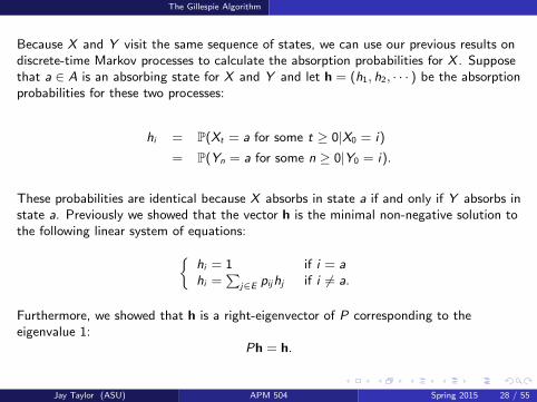
Because X and Y visit the same sequence of states, we can use our previous results ondiscrete-time Markov processes to calculate the absorption probabilities for X . Supposethat a ∈ A is an absorbing state for X and Y and let h = (h1, h2, · · · ) be the absorptionprobabilities for these two processes:

hi = P(Xt = a for some t ≥ 0|X0 = i)

= P(Yn = a for some n ≥ 0|Y0 = i).

These probabilities are identical because X absorbs in state a if and only if Y absorbs instate a. Previously we showed that the vector h is the minimal non-negative solution tothe following linear system of equations:

hi = 1 if i = ahi =

∑j∈E pijhj if i 6= a.

Furthermore, we showed that h is a right-eigenvector of P corresponding to theeigenvalue 1:

Ph = h.



We can also express the absorption probabilities in terms of the rate matrix Q. Indeed,if we multiply the identity hi =

∑j pijhj by qi and then subtract qihi from both sides,

we arrive at the following system of linear equations:

ha = 1∑j∈E

qijhj = 0.

Since the second equation holds even when i = a (since qaj = 0 for all j ∈ E if a is anabsorbing state), it follows that h is a right-eigenvector of the rate matrix witheigenvalue 0:

Qh = 0

where 0 is a column vector indexed by E with all entries equal to 0.


Kolmogorov Equations

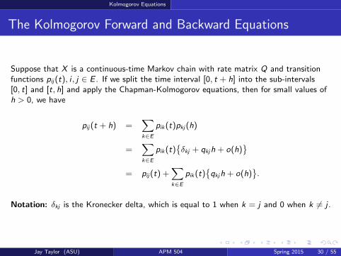
The Kolmogorov Forward and Backward Equations

Suppose that X is a continuous-time Markov chain with rate matrix Q and transitionfunctions pij(t), i , j ∈ E . If we split the time interval [0, t + h] into the sub-intervals[0, t] and [t, h] and apply the Chapman-Kolmogorov equations, then for small values ofh > 0, we have

pij(t + h) =∑k∈E

pik(t)pkj(h)

=∑k∈E

pik(t)δkj + qkjh + o(h)

= pij(t) +

∑k∈E

pik(t)qkjh + o(h)

.

Notation: δkj is the Kronecker delta, which is equal to 1 when k = j and 0 when k 6= j .



By rearranging terms and taking the limit as h ↓ 0, we find that the transitionprobabilities pij(t), i , j ∈ E satisfy the following system of linear ODE’s,

p′ij(t) = limh→0+

pij(t + h)− pij(t)

h=∑k∈E

pik(t) · qkj

which are known variously as the Kolmogorov forward equations, the masterequations, or the Fokker-Planck equations.

Remark: These are called the forward equations because they ‘peek’ forward in timefrom the intermediate states k to the present state j .



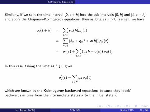
Similarly, if we split the time interval [0, t + h] into the sub-intervals [0, h] and [h, t + h]and apply the Chapman-Kolmogorov equations, then as long as h > 0 is small, we have

pij(t + h) =∑k∈E

pik(h)pkj(t)

=∑k∈E

(δik + qikh + o(h)) pkj(t)

= pij(t) +∑k∈E

(qikh + o(h)) pkj(t).

In this case, taking the limit as h ↓ 0 gives

p′ij(t) =∑k∈E

qikpkj(t)

which are known as the Kolmogorov backward equations because they ‘peek’backwards in time from the intermediate states k to the initial state i .



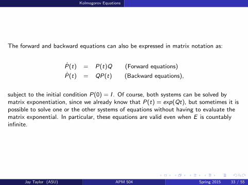
The forward and backward equations can also be expressed in matrix notation as:

P(t) = P(t)Q (Forward equations)

P(t) = QP(t) (Backward equations),

subject to the initial condition P(0) = I . Of course, both systems can be solved bymatrix exponentiation, since we already know that P(t) = exp(Qt), but sometimes it ispossible to solve one or the other systems of equations without having to evaluate thematrix exponential. In particular, these equations are valid even when E is countablyinfinite.



The next theorem tells us how to solve for the marginal distributions of acontinuous-time Markov chain.

Marginal distribution of a CTMCSuppose that X is a continuous-time Markov chain with rate matrix Q and initialdistribution ν = (ν1, ν2, · · · ) on the state space E . Then the marginal distributionspj(t) = Pν(X = j) solve the following initial value problem:

pj(t) =∑i∈E

qijpi (t),

with pj(0) = νj .

Proof: We first observe that the marginal distributions can be written as mixtures of thetransition probabilities with weights provided by the initial distribution:

pj(t) = P(Xt = j |X0 ∼ ν) =∑k∈E

νkP(Xt = j |X0 = k) =∑k∈E

νkpkj(t).



Then, upon differentiating with respect to t and using the forward equation, we have:

pj(t) =∑k∈E

νk pkj(t)

=∑k∈E

νk∑i∈E

pki (t)qij

=∑i∈E

qij∑k∈E

νkpki (t)

=∑i∈E

qijpi (t).



These equations can also be interpreted as a conservation law for probability mass.Indeed, if the j ’th equation is rewritten in the form

pj(t) =∑i 6=j

qijpi (t)− |qjj |pj(t),

then we see that the rate of change in the probability mass occupying state j is equal tothe difference between the rate at which probability mass enters this state minus therate at which probability mass exits this state. This holds because the total probabilitymass must be 1 at all times, giving

0 =

∑j∈E

pj(t)

′ =∑j∈E

pj(t),

so that probability mass can only be moved around the state space, not created ordestroyed.



Example: Suppose that X is a Markov chain with values in a set containing just twostates 1, 2 and that the rate matrix of X is

Q =

(−a ab −b.

).

In other words, X simply alternates between these two states, possibly at different rates.If p(t) = (p1(t), p2(t)) is the marginal distribution of X (t), then

p1(t) = bp2(t)− ap1(t)

p2(t) = ap1(t)− bp2(t)

subject to the initial conditions p1(0) = ν1 and p2(0) = ν2. However, as we also knowthat p1(t) + p2(t) = 1, we can reduce this system to a single equation

p1(t) = b − (a + b)p1(t)

which has solution

p1(t) =b

a + b+ν1a− ν2b

a + be−(a+b)t .


Stationary Distributions


DefinitionLet X be a continuous-time Markov chain with rate matrix Q and state space E . Adistribution π = (π1, π2, · · · ) on E is said to be a stationary distribution for X if

πQ = 0

i.e., π is a left eigenvector for Q corresponding to 0.

Observe that if X0 ∼ π, where π is a stationary distribution, then the marginaldistribution pt of the chain at time t is

pt = πeQt = π∞∑n=0

1

n!Qntn = π

(I + Qt +

1

2Q2t2 + · · ·

)= π,

for every t ≥ 0.



The condition πQ = 0 can also be understood in terms of conservation of mass. If wewrite this condition in terms of the individual components of π and Q, we obtain

0 =∑j∈E

πjqji

=∑j 6=i

πjqji + πiqii

=∑j 6=i

πjqji − πi |qii |

which asserts that, at equilibrium, the total rate at which probability mass flows intostate i must be balanced by the rate at which probability mass flows out of that state:∑

j 6=i

πjqji = πi |qii |.

In particular, a stationary distribution π is also a stationary solution of the Kolmogorovforward equation.



Suppose that X is a continuous-time Markov chain with rate matrix Q = (qij) and let Ybe its jump chain with transition matrix P = (pij). Here we will assume that X has noabsorbing states so that pij = qij/|qii | if j 6= i and pii = 0.

As a general rule, X and Y will not have the same stationary distributions, althoughtheir stationary distributions will be related to one another. For example, if π is astationary distribution for X , then we can define another probability distributionµ = (µ1, µ2, · · · ) on E by setting

µi =qiπi

q

provided that the average jump rate

q =∑j∈E

πj |qjj |

is finite. Division by q guarantees that µ is a probability distribution on E .



I claim that µ is a stationary distribution for the jump chain Y . To verify this, we needto show that µP = µ, which we can do componentwise:

(µP)i =∑j∈E

µjpji

=∑j 6=i

(qjπj

q

)(qjiqj

)=

1

q

∑j 6=i

πjqji

=1

qπiqi = µi .

Notice that the two distributions will be equal only if qi = q for all i ∈ E , i.e., only if Xjumps out of each state at the same rate. Otherwise, the probabilities πi will beinversely proportional to the jump rates qi , with X spending proportionately less time instates with high jump rates than the jump process Y .



Example: We previously showed that if X is the two-state continuous-time Markovchain with rate matrix

Q =

(−a ab −b.

),

and initial distribution ν = (ν1, ν2), then the marginal distribution p(t) of X at timet ≥ 0 is equal to

p1(t) =b

a + b+ν1a− ν2b

a + be−(a+b)t

p2(t) =a

a + b− ν1a− ν2b

a + be−(a+b)t .

Letting t →∞, we see that if a, b > 0, then p(t) converges to the distribution

π =

(b

a + b,

a

a + b

),

which is the unique stationary distribution for this Markov chain.



Example: Recall that the rate matrix and the corresponding transition matrices for theJukes-Cantor model are

Q =

−3µ µ µ µµ −3µ µ µµ µ −3µ µµ µ µ −3µ

,

and

P(t) = eQt =1

4

1 + 3e−4µt 1− e−4µt 1− e−4µt 1− e−4µt

1− e−4µt 1 + 3e−4µt 1− e−4µt 1− e−4µt

1− e−4µt 1− e−4µt 1 + 3e−4µt 1− e−4µt

1− e−4µt 1− e−4µt 1− e−4µt 1 + 3e−4µt

.

Letting t →∞, we see that pxy (t)→ 1/4 for every x , y ∈ T ,C ,A,G and thatπ = (1/4, 1/4, 1/4, 1/4) is a stationary distribution for Q.



In the two examples just presented, we saw that the transition probabilities tended tothe unique stationary distribution of the Markov chain at large times and irrespective ofthe initial state: pij(t)→ πj as t →∞. Although not all continuous-time Markov chainshave this property, the next theorem asserts that a fairly large class of chains do behavein this manner.

TheoremLet X be a continuous-time Markov chain with bounded rate matrix Q and supposethat the jump chain Y is irreducible and that X has a stationary distribution π. Thenfor all states i , j ∈ E ,

limt→∞

pij(t) = πj .

In particular, it follows that π is the unique stationary distribution of X and that themarginal distributions of the variables Xt tend to π as t →∞ for all initial distributionsof X0.



Example: Continuous-Time Birth-Death Processes

A continuous-time Markov chain X is said to be a continuous-time birth-death processif the state space is E = 0, 1, · · · ,N, where N may be finite or infinite, and the ratematrix Q is tridiagonal, i.e.,

qij =

λi if j = i + 1µi if j = i − 1

−(µi + λi ) if j = i0 if |j − i | > 1,

with µ0 = λN = 0. Often we think of λi and µi as the total birth rate and total deathrate, respectively, in a population containing i individuals. As with their discrete-timecousins, the simple structure of the rate matrix of a continuous-time birth-deathprocesses can often be exploited when performing calculations.



By way of example, suppose that X is a continuous-time birth-death process and that

µi > 0 and λi−1 > 0 for i = 1, · · · ,N,and

N∑i=1

λ0λ1 · · ·λi−1

µ1µ2 · · ·µi<∞.

If these conditions are satisfied, then it can be shown that X has a unique stationarydistribution π = (π0, π1, π2, · · · ) on E . Since πQ = 0, it follows that these probabilitiesmust satisfy the following system of equations:

0 = −λ0π0 + µ1π1

0 = λi−1πi−1 − (λi + µi )πi + µi+1πi+1, 1 ≤ i < N

0 = λN−1πN−1 − µNπN (if N <∞).



These equations can be solved recursively as follows. Starting with i = 0, we have

π1 =λ0

µ1π0

Then with i = 1,

π2 =1

µ2

(λ1 + µ1)π1 − λ0π0

=

1

µ2λ1π1

=λ0λ1

µ1µ2π0.

Continuing in this way, one finds that for general i = 1, · · · ,N,

πi =λ0λ1 · · ·λi−1

µ1µ2 · · ·µiπ0.



For π to be a probability distribution on E , these quantities must sum to 1:

1 =N∑i=0

πi = π0

(1 +

N∑i=1

λ0λ1 · · ·λi−1

µ1µ2 · · ·µi

)

which gives

π0 =

(1 +

N∑i=1

λ0λ1 · · ·λi−1

µ1µ2 · · ·µi

)−1

> 0

since our second condition on the birth and death rates guarantees that the sum insidethe parentheses is finite even if N is infinite. This will be true, for example, if there is anε > 0 and a positive integer K such that λi < (1− ε)µi for all i ≥ K , i.e., at sufficientlyhigh densities, the birth rates need to be geometrically less than the death rates.Otherwise, the population might grow without bound, in which case there need not be astationary distribution.


Poisson Processes

Poisson Processes

Let η1, η2, · · · be a sequence of independent exponentially-distributed random variableswith rate λ and define a new sequence of random variables N = (Nt ; t ≥ 0), withcontinuous time parameter t, by

Nt = supn ≥ 0 : η1 + · · ·+ ηn < t.

The process N defined in this manner is said to be a Poisson process with rate λ andis a continuous-time Markov chain with values in E = 0, 1, · · · . It is often interpretedin the following manner. Think of ηi as the random waiting time between successiveevents and let

Tn = η1 + · · ·+ ηn

be the time of the n’th event. Then Nt is the number of events that have occurred upto time t.


Poisson Processes

To calculate the distribution of Nt , we need to recall that the distribution of a sum of ni.i.d. exponential random variables with parameter λ is the Gamma distribution withparameters n and λ. Then, since

Nt = n = Tn ≤ t < Tn + ηn+1

it follows that

P(Nt = n) = P(Tn ≤ t < Tn + ηn+1)

=

∫ t

0

P(Tn = s)P(ηn+1 > t − s)ds

=

∫ t

0

λn

Γ(n)sn−1e−λse−λ(t−s)ds

= e−λtλn

(n − 1)!

∫ t

0

sn−1ds

= e−λt(λt)n

n!.

Since this holds for every n ≥ 0, it follows that Nt is Poisson-distributed with parameterλt. Of course, this is also the source of the name of this process.


Poisson Processes

With some additional work, it can be shown that the process N also has the followingproperties:

1 N has independent increments: for all 0 ≤ t0 < t1 < · · · < tk , the randomvariables Nt0 , Nt1 − Nt0 , Nt2 − Nt1 , · · · ,Ntk − Ntk−1 are independent.

2 For each t > 0,

P(Nt+δt = n + 1|Nt = n) = λδt + o(δt)

P(Nt+δt = n|Nt = n) = 1− λδt + o(δt)

P(Nt+δt = i |Nt = n) = o(δt), for every i 6= n, n + 1.

Both of these properties follow from the fact that N is a Markov process. The firstproperty asserts that the numbers of events occurring in disjoint time intervals areindependent; in fact, this is stronger than the Markov property. The second propertyasserts that the probability of having more than one jump in any short time interval isnegligibly small. It also asserts that the rate of jumps from n to n + 1 is equal to λ.


Poisson Processes

The marginal distributions of a Poisson process N = (Nt : t ≥ 0) can also be found bysolving the forward equation. Recall that the transition rates for this process are

qij =

λ if j = i + 1−λ if j = i

0 otherwise.

By convention, we set N0 = 0 (i.e., no events have occurred at time 0), so that themarginal distribution of Nt is given by the transition probabilities p0n(t). The forwardequation for this process take the following form:

p00(t) = −λp00(t)

p0n(t) = λp0,n−1(t)− λp0n(t), n > 0,

with initial conditionp0n(0) = δ0n.


Poisson Processes

The first equation only involves p00(t) and can be solved immediately to give

p00(t) = e−λt .

In contrast, the subsequent equations involve both p0n(t) and p0,n−1(t) and will lead toa recursion. Since the equation satisfied by p0n(t) is a first-order linear differentialequation, it can be solved by first multiplying both sides by the integrating factor eλt

and then rearranging so that we obtain

eλt p0n(t) + λeλtp0n(t) = λeλtp0,n−1(t).

Notice that the left-hand side is now an exact differential, i.e.,(eλtp0n(t)

)′= λeλtp0,n−1(t),

which can be integrated (using the fact that p0n(0) = 0 when n > 0) to give

p0n(t) = e−λtλ

∫ t

0

eλsp0,n−1(s)ds.


Poisson Processes

This last equation allows us to calculate p0n(t) once we know p0,n−1(t). However, sincewe already know that p00(t) = e−λt , we can solve recursively for all of the probabilitiesp0n(t) by calculating these integrals. For example,

p01(t) = e−λtλ

∫ t

0

eλse−λsds = e−λtλt.

Similarly,

p02(t) = e−λtλ

∫ t

0

eλse−λsλsds = e−λt(λt)2

2,

and

p03(t) = e−λtλ

∫ t

0

eλse−λsλ2s2

2ds = e−λt

(λt)3

3!.


Poisson Processes

This leads us to conjecture that

p0n(t) = e−λt(λt)n

n!,

which can be confirmed by induction since

p0,n+1(t) = e−λtλ

∫ t

0

eλse−λs(λs)n

n!ds = e−λt

(λt)n+1

(n + 1)!.

Thus, as shown previously using a very different approach, we see that the marginaldistribution of Nt is Poisson with parameter λt.


Date post:	01-Sep-2018
Category:	Documents
Upload:	truongque
View:	217 times
Download:	0 times

APM 504: Continuous-time Markov Chainsjtaylor/teaching/Spring2015/APM504/... · APM 504:...

Documents