The Astrophysical Journal, 770:36 (11pp), 2013 June 10 doi:10.1088/0004-637X/770/1/36C© 2013. The American Astronomical Society. All rights reserved. Printed in the U.S.A.

APOSTLE: LONGTERM TRANSIT MONITORING AND STABILITY ANALYSIS OF XO-2b

P. Kundurthy1, R. Barnes1,2, A. C. Becker1, E. Agol1, B. F. Williams1, N. Gorelick3, and A. Rose11 Astronomy Department, University of Washington, Seattle, WA 98195, USA

2 Virtual Planetary Laboratory, Seattle, WA 98195, USA3 Google Inc., Mountain View, CA 94043, USA

Received 2012 November 29; accepted 2013 April 25; published 2013 May 22

ABSTRACT

The Apache Point Survey of Transit Lightcurves of Exoplanets (APOSTLE) observed 10 transits of XO-2b over aperiod of 3 yr. We present measurements that confirm previous estimates of system parameters like the normalizedsemi-major axis (a/R�), stellar density (ρ�), impact parameter (b), and orbital inclination (iorb). Our errors on systemparameters like a/R� and ρ� have improved by ∼40% compared to previous best ground-based measurements.Our study of the transit times show no evidence for transit timing variations (TTVs) and we are able to rule outco-planar companions with masses �0.20 M⊕ in low order mean motion resonance with XO-2b. We also exploredthe stability of the XO-2 system given various orbital configurations of a hypothetical planet near the 2:1 meanmotion resonance. We find that a wide range of orbits (including Earth-mass perturbers) are both dynamically stableand produce observable TTVs. We find that up to 51% of our stable simulations show TTVs that are smaller thanthe typical transit timing errors (∼20 s) measured for XO-2b, and hence remain undetectable.

Key words: eclipses – methods: numerical – planetary systems – planets and satellites: fundamental parameters –planets and satellites: individual (XO-2b)

Online-only material: color figures, machine-readable tables

1. INTRODUCTION

Observational efforts on two fronts (ground-based and space-based) have revealed a great diversity in the properties ofplanets (and planet candidates), and posed several new questionsabout the planet formation process. The search for planetsand the careful measurement of planetary properties are theobservational foundations upon which the physics of planetformation may be understood. The exoplanet community hasco-opted the term “architecture” to embody several propertiesof planetary systems such as multiplicity and orbital parameterslike eccentricities (e), inclinations (iorb), semi-major axes (a),and orbital periods. The distributions of individual planetaryproperties like masses and radii (Mp and Rp, respectively) mayalso be included in this term. The primary goal of the ApachePoint Observatory Survey of Transit Lightcurves of Exoplanets(APOSTLE) is to catalog transit light curves at high precisionin order to (1) measure system parameters and (2) look fortransit timing variations (TTVs) that may indicate the presenceof additional planets.

The transit technique applies to those systems where theorbital inclination of an exoplanet is close to 90◦ (i.e., edge-on) with respect to the observer’s sky-plane (see the discoverypaper Charbonneau et al. 2000). In this case, the observer sees au-shaped dip in the starlight caused when the planet eclipses thestar (Winn 2011). The objective of several ground-based andspace-based efforts focused on transit observations is to catalogand improve measurements of system parameters, which in turngives us an improved picture of the architecture of the planetarysystem. This process is key toward developing theories of planetformation that can adequately explain the origin and evolutionof all planetary systems (including our own).

The APOSTLE target XO-2b is a Hot-Jupiter on a 2.6 dayorbit around an early type K dwarf (V = 11.2; Burke et al.2007). The planet is known to have a mass of 0.555 MJup anda radius of 0.992 RJup (Southworth 2010). The system is not

known to have any other planet-mass objects. However, Naritaet al. (2011) claim to detect long-term radial velocity varia-tion that deserves further follow-up. Transit timing measure-ments from the ground are consistent with a linear ephemeris(Fernandez et al. 2009; Sing et al. 2011; Crouzet et al. 2012),although the cited studies note that there are statistically sig-nificant deviations in the measurement of the orbital periods.A search for additional eclipses using the EPOXI mission byBallard et al. (2011) had inconclusive results since the eclipsewas not fully sampled. Spitzer observations of the secondaryeclipse of XO-2b show IRAC 3.6, 4.5, and 5.8 μm fluxeswhich are consistent with the presence of a temperature in-version (Machalek et al. 2009). There have also been detectionsof optical absorbers in the planetary atmosphere such as potas-sium from narrow band optical transmission spectrophotometry(Sing et al. 2011). Early theoretical studies indicated that stel-lar insolation levels directly influenced the presence or absenceof a thermal inversion layer (depending on the survival of at-mospheric absorbers; Hubeny et al. 2003; Burrows et al. 2007;Fortney et al. 2008). The planetary atmosphere classificationsystem developed by Fortney et al. (2008) places XO-2b in antransition zone between planets with (pM) and without (pL) ther-mal inversions. XO-2b is one of a handful of Hot-Jupiters in thisregion. However, observational evidence suggests (Machaleket al. 2008) that more complicated models need to be con-sidered. Irradiation from stellar activity may need to be in-cluded (Knutson et al. 2010) and atmospheric chemistry mayalso need to be considered to provide a more complete picture(Madhusudhan 2012). The host star of the XO-2 system isknown to be a high metallicity ([Fe/H] = 0.45 ± 0.02), highproper motion star (μTot = 157 mas yr−1) in a visual binary(Burke et al. 2007). Spectral activity indices show that XO-2 isfairly inactive compared to other stars of similar spectral type(Knutson et al. 2010).

A primary goal of APOSTLE and other campaigns thatmonitor transiting exoplanets is to search for TTVs that reveal

1

The Astrophysical Journal, 770:36 (11pp), 2013 June 10 Kundurthy et al.

Table 1APOSTLE Observing Summary for XO2

T# UTD Obs. Cond. Filter Exp. Bin Phot. Ap. RMS (ppm) %Rej. Flux Norm. Error Scaling(1) (2) (3) (4) (5) (6) (7) (8) (9) (10) (11)

1 2008-01-09 Clear I 0.5 45 13 557 3% 0.9561 1.17402 2008-02-12 Clear I 0.5 45 24 510 <1% 0.9561 1.31293 2008-03-04 Clear I 0.5 45 15 411 <1% 0.9632 1.25104 2008-11-23 Poor Weather I 10, 25, 45 45 27 939 1% 0.9756 2.74825 2009-02-07 Poor Weather I 45 . . . 31 1085 11% 0.9721 2.98686 2009-03-13 Poor Weather I 45 . . . 46 405 11% 0.9766 1.23567 2010-10-25 Clear r ′ 45 . . . 35 553 2% 0.9676 2.27608 2010-12-27 Poor Weather r ′ 45 . . . 43 775 5% 0.9643 3.00929 2011-01-30 Clear r ′ 45 . . . 48 354 1% 0.9646 1.457110 2011-03-05 Clear r ′ 45 . . . 43 693 <1% 0.9660 2.7990

Notes. Column 1: transit number; Column 2: universal time date; Column 3: observing conditions; Column 4: observing filter; Column 5: exposure time (seconds);Column 6: bin size in seconds; Column 7: optimal aperture radius (pixels); Column 8: scatter in the residuals; Column 9: % frames rejected due to saturation or othereffects; Column 10: flux normalization between the target and comparison star; Column 11: the factor by which the photometric errors were scaled.

the presence of unseen companions (Agol et al. 2005; Holman& Murray 2005). In principle, Earth-mass planets in or nearmean motion resonances could perturb the orbit of the transitingplanet enough to produce a sinusoidal oscillation in the mid-points of transits. However, the full range of stable orbits thatcan produce a detectable TTV signal has never been explored.The detection of TTVs by Kepler (e.g., Holman et al. 2010)has demonstrated that stable systems are capable of producingTTVs, and other studies have explored a limited range ofarchitectures (Haghighipour & Kirste 2011), but the systematicexploration of parameter space of an Earth-mass planet in orbitnear a hot Jupiter has not been undertaken. Here we examine3.6 million possible masses and orbits of an approximatelyEarth-mass planet orbiting in or near the 2:1 outer mean motionresonance through N-body simulations. We find that stable orbitsthat also produce detectable TTVs do exist in the XO-2 system,and hence can exist in similar Hot-Jupiter systems.

In this paper we report observations of 10 transits of XO-2b,taken as part of APOSTLE. In Section 2 we outline our obser-vations. In Section 3 we briefly outline (1) the data reduction,photometry (Section 3.1), (2) the transit model (Section 3.2)and light curve fitting (Section 3.3); both processes have alsobeen described in previous work (Kundurthy et al. 2013). InSection 4 we present our estimates of the system parameters forXO-2b and in Sections 4.1 and 4.2 we present results fromour study of transit depth variations (TDVs) and TTVs. InSection 5 we present results form N-body simulations usedto study the stability of hypothetical planetary configurationsat the 2:1 mean-motions resonance. Finally, in Section 6 wesummarize our findings.

2. OBSERVATIONS

XO-2b was observed by members of the APOSTLE teamon 10 occasions over a timespan of 3 yr from early 2008 untilthe spring of 2011. All observations of XO-2 were carried outusing AGILE, a high-speed frame-transfer CCD (Mukadam et al.2011), on the ARC4 3.5 m telescope at Apache Point, NewMexico. The summary of observations is given in Table 1. XO-2was an early APOSTLE target and was observed using a varietyof instrumental settings, as the team had not converged on anoptimal observing strategy prior to 2010. Early observationswere made in the I-band (λ0 = 805 nm; Cousins 1976; Bessell

4 Astrophysical Research Consortium.

1990) with several data sets taken with short read-out (exposuretimes, Column 5 in Table 1). The short read-out mode allowedfor fine sampling of the light curve, but, due to the lower signal-to-noise and the unsuitability for characterizing systematics,this observing mode was abandoned. In addition, the I-bandimages also contained a strong contribution from a fringe patterndue interference from the backscattering of atmospheric lineswithin the CCD’s pixels. The removal of this fringe pattern isdiscussed in Section 3.1. Early in 2010, the observing strategychanged to longer readouts (typically 45–75 s) to reduce thelevel of correlated noise (red-noise), and were made using ther ′-band which is similar to the SDSS5 r filter (λ0 = 626 nm;Fukugita et al. 1996), to reduce the influence of fringes. In thelong read-out mode the telescope was defocused to spread thestellar point-spread function (PSF) across multiple pixels, whichminimized the systematics caused by pixel-to-pixel wanderingof the PSF over the imperfect flatfield. The longer exposures alsoallowed for a greater count rate which maximized the signal-to-noise per image. The count rate was kept below AGILE’s non-linearity limit of ∼52k ADU and well below its saturation levelof 61k ADU by small adjustments to the telescope’s secondaryfocus during observations.

XO-2 (TYC 3413-5-1) and its visual binary companionTYC 3413-210-1 (separated by ∼30′′) were the only brightstars that fit in AGILE’s field of view. Both stars are ofidentical spectral type (K0V) and nearly identical brightnessesin the filters used by APOSTLE, with their Johnson R and Imagnitudes at 10.8 and 10.5, respectively (Monet et al. 2003).Our uncalibrated differential photometry also showed goodagreement in their brightnesses, with the out-of-eclipse, un-normalized flux ratios being different by only 4% and 3% inthe I-band and r ′-band, respectively (Column “Flux Norm.”in Table 1). The observations were made over a variety ofobserving conditions (Column “Obs. Conditions” in Table 1).The observing conditions are classified as “Clear” or “PoorWeather” with the former implying good data with few orno interruptions in data collection, and the latter indicatingthat the we experienced cloud cover or poor seeing conditionsresulting in lower quality data. The tabulated transits are thosefor which we were able to capture the whole transit or at least apartial transit. Partial transits are those where portions of the in-eclipse light curve were lost due to bad weather or instrumentalfailure. Several data points were lost for the nights of UTD

5 Sloan Digital Sky-Survey.

2

The Astrophysical Journal, 770:36 (11pp), 2013 June 10 Kundurthy et al.

2008 September 22 (transit 4), 2009 February 6 (transit 5),2009 March 12 (transit 6), and 2010 December 27 (transit 8).However, we do include these nights since we did manage toobtain reasonable portions of the in-eclipse and out-of-eclipsedata, which make it possible to determine transit properties(albeit at a loss of accuracy and precision).

3. DATA ANALYSIS

This section outlines various stages in the analysis of lightcurves, starting with (1) the image reduction and photometry,and (2) the transit model and Markov Chain Monte Carlo(MCMC) analyzer (see also Kundurthy et al. 2013).

3.1. Reduction and Photometry

APOSTLE data were reduced using a pipeline developedspecifically for AGILE images. The pipeline (written in IDL6)performs pixel-by-pixel error propagation, and image process-ing specific to the AGILE CCD. In addition to the standard pho-tometric reduction steps like dark subtraction and flat-fielding,the pipeline performs non-linearity and fringe corrections spe-cific to AGILE. The details on AGILE’s non-linearity correctionare described in Section 3 of Kundurthy et al. (2013). Some ofthe initial observations by APOSTLE were carried out usingshort exposures (see Column 5 “Exp.”) in Table 1. We binnedthese data by averaging the flux ratios in 45 s bins.

For several of the initial XO-2 data taken using AGILE’sI-band, a fringe pattern had to be subtracted to create scienceimages. Photons from strong atmospheric lines (in the I-bandbandpass) backscatter within the CCD pixels, and owing tothe variable thickness of the pixel array, interference betweenthese photons creates the fringe pattern. Since the fringe patternis convolved with the illumination pattern of the CCD, thefringe correction has to be applied after dark-subtraction andflat-fielding. During the initial characterization of the AGILECCD, an empirical fringe frame was produced by mediancombining dithered frames on the dark sky, where the fluxcontributions from stars were removed by outlier rejection. Theresulting combined frame served as a “Model” fringe pattern(F), normalized to have a median of zero, and an amplitude ofone, such that it could be scaled to match the fringe patterns onscience frames. The science frame affected by the fringe pattern(T

′) is assumed to be a linear combination of the fringe-less

science image (T) and a fringe pattern:

T′ = T + a0F, (1)

where F is the model fringe frame and a0 is a scaling factordescribing the amplitude of the fringing on a given frame. Thefringe amplitude is estimated by minimizing χ2 and fitting fora0 in the above model. The corrected images (T = T

′ − a0F ),were found to be sufficiently corrected of fringes after visualexamination. We found the fringe amplitudes (a0) on XO-2science frames to always be smaller than the standard deviation(i.e., scatter) of the global sky background on each frame; a0ranged between 6%–13% of the scatter in the sky for XO-2 data.

We extracted photometry from an optimal circular aperturecentered around the target and comparison stars. In addition weextracted the counts on image products like the master-dark andmaster-flat, to serve as nuisance parameters for detrending, usingthe same aperture and centroids from photometry. The centroids

6 Interactive Data Language.

Table 2Nuisance Parameters Used for XO-2 Nights

T# Nuisance Parameters Used (FLDC, OLDC, and MDFLDC)

T1 airmass, msky1, msky2, gsky, x1, y1, x2, y2, sD1, sD2, sF1, sF2, a0

T2 airmass, msky1, msky2, gsky, x1, y1, x2, y2, sD1, sD2, sF1, sF2, a0

T3 airmass, msky1, msky2, gsky, x1, y1, x2, y2, sD1, sD2, sF1, sF2, a0

T4 airmass, msky1, msky2, gsky, x1, y1, x2, y2, sD1, sD2, sF1, sF2, a0

T5 airmass, x1, y1, sD1, sF1, a0

T6 airmass, x1, y1, sD1, sF1, a0

T7 airmass, gsky, x1, y1, sD1, sF1

T8 airmass, gsky, x1, y1, sD1, sF1

T9 airmass, gsky, x1, y1, sD1, sF1

T10 airmass, gsky, x1, y1, sD1, sF1

Notes. airmass: atmospheric column; (x1, y1), (x2, y2): centriods of Target (1) andComparison (2); msky1, msky2: median sky around Target (1) and Comparison(2); gsky: global median sky; sD1, sD2: sum of counts in aperture on master-dark; sF1, sF2: sum of counts in aperture on master-flat; a0: fringe scaling (seeEquation (1)).

were derived using SExtractor (Bertin & Arnouts 1996), whichallowed for the use of customized donut-shaped convolutionkernels for defocused PSFs. Science frames where pixels insidea photometric aperture exceeded AGILE’s saturation limit of61k were rejected. Images at the other extreme, where thestars were obscured by clouds, and resulted in low signal-to-noise measurements were also rejected (i.e., where individualphotometric errors were >5000 ppm). The fraction of rejectedframes per night is listed in Column 9 “%Rej.” in Table 1.The optimal aperture was selected after extracting photometryon a list of circular apertures with radii between 5–50 pixelsat an interval of 1 pixel. The optimal aperture was selectedwhere the scatter in the residuals of the detrended light curveminus a trial transit model (based on values from the literature)was minimized. The correction function Fcor (or detrendingfunction) is modeled as a linear sum of nuisance parametersas described by the following equation:

Fcor,i =Nnus∑

k=1

ckXk,i , (2)

where Xk,i are the nuisance parameters, ck are the correspondingcoefficients. The index k counts over the number of nuisanceparameters Nnus. The detrending coefficients are chosen byminimizing the χ2 between the observed data (O), a modelfunction (M), and the correction function,

χ2 =Nall∑

j

(Oj − Mj − Fcor,j )2

σ 2j

, (3)

here j is the index which counts over the total number of datapoints (Nall). The observed, model and correction function termsare all in normalized flux ratio units. The list of parameters usedfor detrending each light curve in the XO-2 dataset are presentedin Table 2, with variable definitions given in the footnotes. Asuitable set of detrending parameters were selected for a givennight by running several manual trials of linear least squaresminimization on single transit light curves and its correspondingmodel light curve and correction function (Equation (2)). Themodel parameters were fixed at reasonable values and onlythe coefficients (ck) were fit. Those nuisance parameters whichreturned large uncertainties on the coefficients were excludedsince this indicated a poor match to the noise trend in a

3

The Astrophysical Journal, 770:36 (11pp), 2013 June 10 Kundurthy et al.

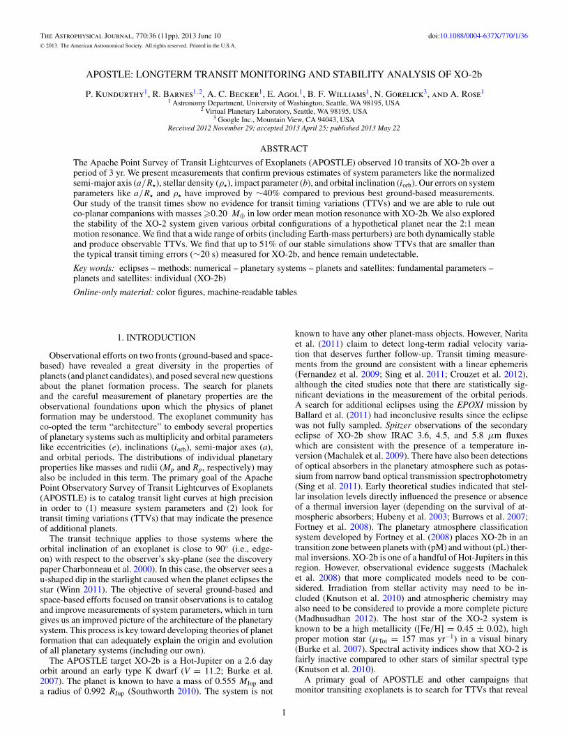
Figure 1. Six I-band and four r ′-band light curves of XO-2b. The vertical axisis in normalized flux ratio units. The horizontal axis shows time from the mid-transit time in days, computed by subtracting the appropriate mid-transit timefor each transit from the best-fit values in the fixed LDC chain.

light curve. This method of selecting nuisance parameters isadmittedly ad-hoc; automated parameter selection techniquescould be applied in the future. The detrending is performedusing the final set of nuisance parameters in conjunction withfitting the transit parameters in order to ensure that the correctionprocess is not biased by the trial model used in the selection ofnuisance parameters.

The 10 transits of XO-2b are shown in Figure 1 in normalizedflux ratios (with offsets for clarity). Shown are the detrendedlightcurves, the corresponding errors, and the best fit transitmodel; the data shown in Figure 1 are listed in Table 3. Theplotted data result from the data reduction and model fittingprocesses described in Sections 3.1–3.3.

3.2. MultiTransitQuick

We developed a transit model called MultiTransitQuick(MTQ) in PYTHON, which is based on the analytic light curvemodels presented in Mandel & Agol (2002), and the PYTHONimplementation of some of its functions (from EXOFAST byEastman et al. 2013). The description of MTQ used for this studyis described in some detail in Kundurthy et al. (2013). MTQcan be used to (1) fit for transit depths for data taken withmultiple filters (Multi-Filter model), or (2) fit each transit depthindividually (Multi-Depth).

Table 3APOSTLE Light Curve Data for XO-2

T# T − T0 Norm. Fl. Ratio Err. Norm. Fl. Ratio Model Data(1) (2) (3) (4) (5)

1 −0.1341616 1.000004100 0.001207284 1.0000000001 −0.1315574 0.999797978 0.001102731 1.0000000001 −0.1305157 0.997707769 0.001047412 1.0000000001 −0.1299949 0.999906661 0.001190794 1.0000000001 −0.1289532 0.998693635 0.001118320 1.0000000001 −0.1279116 0.998939727 0.001098241 1.0000000001 −0.1273907 0.999021973 0.000987372 1.0000000001 −0.1268699 1.001381660 0.001209313 1.0000000001 −0.1263491 0.998899046 0.001076096 1.0000000001 −0.1258282 1.001212353 0.001160014 1.000000000. . . . .. . . . .

Notes. Column 1: transit number; Column 2: time stamps − mid transit times(BJD); Column 3: normalized flux ratio; Column 4: error on normalized fluxratio; Column 5: model data.

(This table is available in its entirety in a machine-readable form in the onlinejournal. A portion is shown here for guidance regarding its form and content.)

The set of parameters used for Multi-Filter version of MTQ isθMulti-Filter = {tT , tG, Dj...NF

, v1,j...NF, v2,j...NF

, Ti...NT}, where tT

is transit duration, tG is the limb-crossing duration and Ti are themid-transit times. The filter-dependent parameters include thetransit depth Dj and the limb-darkening parameters v1,j and v2,j

described in Kundurthy et al. (2013). The subscripts i...NT andj...NF are used to denote multiple transits (NT ) and multiplefilters (NF) respectively. The XO-2 data were gathered using theI-band and r ′-band, where NF was 2 and the number of transitsNT was 10.

The parameter set is only slightly different for the Multi-Depth version, with θMulti-Depth = {tT , tG, Di...NT

, v1,j...NF,

v2,j...NF, Ti...NT

}; the difference being the transit depth is nowfit for each transit separately instead of each filter. The filtersare still tracked to ensure the use of the correct limb-darkeningparameters for each light curve. A single light curve is set as the“reference” light curve and used to internally compute severalorbital parameters. For the XO-2 data set we used transit 3since it had few gaps, and had the best photometric precisionamong the I-band light curves. We did not use an r ′-band lightcurve as a reference since this filter is more affected by limb-darkening when compared to the I-band and hence estimates ofthe planet-to-star size ratio (Rp/R�) (used in the computation oforbital parameters) may be susceptible to degeneracies. Usingthe Multi-Depth model aids in understanding transit depthvariations over multiple epochs.

3.3. Transit MCMC

We developed a MCMC analyzer called Transit MCMC(TMCMC), based on the Metropolis–Hastings algorithm (Gelmanet al. 2003; Tegmark et al. 2004; Ford 2005), with an adaptivestep-size modifier (Collier Cameron et al. 2007). MCMC rou-tines quantify the uncertainty distributions of model parameters(given the data) using Bayes’ theorem, by sampling parameterspace such that samples from high probability regions (low χ2)are selected at a greater rate than those from low probability re-gions. The final ensemble of sampled points the MCMC routinetypically represent the uncertainty distributions of the modelparameters. One must note that adaptive MCMCs are generallynot considered to be truly Markovian in nature and their results

4

The Astrophysical Journal, 770:36 (11pp), 2013 June 10 Kundurthy et al.

Table 4TMCMC Chains for XO-2

Chain Model Vector Nfree Chain Length Corr. Length Eff Length χ2 DOF

FLDC θMulti-Filter 14 1,900,001 100 19,000 3272.94 3312OLDC θMulti-Filter 18 1,900,001 4,949 383 3268.48 3308MDFLDC θMulti-Depth 22 1,900,001 588 3,231 3197.53 3304

are valid only if adaptation diminishes with time (Roberts &Rosenthal 2009); a property that our chains do display.

For APOSTLE data sets, we explored system parametersusing three different kinds of chains. Two of these werebased on the Multi-Filter parameter set θMulti-Filter describedin Section 3.2 and the third used the Multi-Depth parame-ter set (θMulti-Depth). The two Multi-Filter chains used fixedlimb-darkening coefficients (LDC) and open limb-darkeningcoefficients (OLDC). For the fixed LDC chains (FLDC), thecoefficients were simply fixed to values tabulated for the ap-propriate observing filter (Claret & Bloemen 2011). For theOLDC chains, the limb-darkening parameters v1 and v2, forboth I-band and r ′-band data, are allowed to float. The abil-ity to constrain stellar limb-darkening requires high precisiondata, such as those collected using the Hubble Space Telescope(Brown et al. 2001; Knutson et al. 2007). Previous attempts to fitfor limb-darkening on APOSTLE data have resulted in Markovchains that failed to converge (Kundurthy et al. 2011, 2013).The third type of Markov chain was run on the Multi-Depthparameter set θMulti-Depth described in Section 3.2. APOSTLElight curves were gathered over a long time-baseline, and sta-tistically significant depth variations seen in the data may helpshed light on the various phenomena responsible for depth vari-ations (see Section 3.2), or point to limitations in the data andmodel.

Several of the preliminary steps for executing a chain usingTMCMC are described in (Kundurthy et al. 2013). These steps in-clude (1) setting bounds and (2) running short single-parameterexploratory chains to determine a set of suitable starting jump-sizes for the long Markov Chains. We ran long chains of 2×106

steps from two different starting locations for each model sce-nario: FLDC, OLDC, and Multi-Depth/FLDC. After comple-tion we (1) cropped the initial stages of these chains to removethe burn-in phase, where the chain is far from the best-fit re-gion, and (2) we exclude the stage where the chain is far fromthe optimal acceptance rate of 23% ± 5% (as noted for multi-parameter chains; Gelman et al. 2003). We run three types ofpost-processing on the chains after cropping: (1) We computethe ranked and unranked correlations in the chains of everyfit parameter with respect to the others. These statistics pro-vide an estimate of the level of degeneracy between parame-ters in a given model. The next post-processing steps are twocommonly used diagnostics to check for chain convergence,namely (2) computing the auto-correlation lengths and (3) theGelman–Rubin R-static values (Gelman & Rubin 1992). Theauto-correlation lengths determine the scale over which a chainhas local trends. From the auto-correlation length one can com-pute the effective length as the total chain length divided by theauto-correlation length, which represents the statistical signifi-cance with which the uncertainty distribution was sampled. Alarge effective length (>1000) represents a well-sampled distri-bution. The R-statistic represents the level of coverage the chainhas over the parameter space. When parameter space has beenproperly sampled the R-statistic computed using chains fromdifferent starting locations will be close to 1. We deem those

chains as converged that have an effective length >1000 and anR-statistic within 10% of 1.

3.3.1. TAP

The Transit Analysis Package (TAP; Gazak et al. 2012)implements the red-noise model of Carter & Winn (2009),who find that models that do not fit for red-noise are subjectto inaccuracies in transit parameters on the order of 2σ–3σand tend to have underestimated errors by up to 30%. Fortransit timing studies, poor estimates such as these are causefor concern, since smaller errors and large deviations fromthe expected time can easily lead to false claims of TTVs.Since TMCMC does not include red-noise analysis we run fitson APOSTLE light curves using TAP as a check to the resultsderived from TMCMC.

The typical TAP parameter set is: θTAP = {a/R�, iorb,(Rp/R�)i...NF

, Ti...NT, σ(white,i...NT ), σ(red,i...NT )}, where a/R�,

iorb and (Rp/R�) are the commonly fit transit parametersdenoting the semi-major axis (in stellar radius units), the orbitalinclination and the planet-to-star radius ratio, respectively. Thenoise analysis parameters σ(white,i...NT ) and σ(red,i...NT ) are thewhite-noise and red-noise levels for NT transits respectively.The TAP package does not fit for the period using the transittimes, and often yields poor estimates of the period, so we fixedthe period to the value derived from TMCMC. The limb-darkeningwas fixed to values from the literature. The orbital eccentricity(e) and argument of periastron were kept fixed at 0 for XO-2b.

4. SYSTEM PARAMETERS

This section describes results from our execution of thetwo chains for the parameter set θMulti-Filter, and one for theθMulti-Depth described in Section 3.3. Post processing statisticsand other data for these chains are listed in Table 4. The columns“Nfree,” “Chain Length,” “Corr. Length” and “Eff. Length” listthe number of free parameters, the length of the cropped chain,the correlation and effective lengths, respectively. All chainswere run for approximately 2 million steps, but about 100,000of the initial steps were removed to account for “burn-in” andselection rate stabilization. The XO-2b chain with OLDC hasa low effective length indicating poor Markov chain statistics.The FLDC chains (both θMulti-Filter and θMulti-Depth) model satisfythe condition of a well sampled posterior distribution (effectivelength is >1000). The final two columns list the goodness offit (i.e., lowest χ2 in the MCMC ensemble) and degrees-of-freedom (DOF) from the respective chain. Parameters from allchains had Gelman–Rubin R-statistics close to 1 indicating thatthe parameter space was covered evenly (though the OLDCchain was not sampled finely enough, based on the auto-correlation data).

The resulting best-fit parameter estimates are listed in Table 5for the Multi-Filter models, and in Table 6 for the Multi-Depthmodels. These tables also list the derived system parameters.The transformation between the MTQ parameters to the derivedsystem parameters are described in Carter et al. (2008) and

5

The Astrophysical Journal, 770:36 (11pp), 2013 June 10 Kundurthy et al.

Table 5XO-2 Parameters for θMulti-Filter

Parameter FLDC OLDC Unit

MTQ Parameters

tG 0.0107 ± 0.0002 0.0108 ± 0.0002 daystT 0.1008 ± 0.0001 0.1004 ± 0.0002 daysD(I ) 0.0126 ± 0.0001 0.0126 ± 0.0001 . . .

D(r ′) 0.0130 ± 0.0001 0.0131 ± 0.0001 . . .

v1(I ) (0.5944) 0.5440 ± 0.0313 . . .

v1(r ′) (0.6980) 0.6411+0.0332−0.0249 . . .

v2(I ) (0.1452) 0.2806 ± 0.0904 . . .

v2(r ′) (0.3524) 0.4786+0.0734−0.0992 . . .

Derived Parameters

(Rp/R�)(I ) 0.1030 ± 0.0003 0.1033 ± 0.0004 . . .

(Rp/R�)(r ′) 0.1024 ± 0.0003 0.1029 ± 0.0004 . . .

b 0.17+0.04−0.02 0.21 ± 0.03 . . .

a/R� 8.14 ± 0.06 8.11 ± 0.07 . . .

iorb 88.79 ± 0.15 88.53+0.02−0.10 (deg)

ν/R� 19.55 ± 0.15 19.48 ± 0.17 days−1

ρ� 1.49 ± 0.03 1.48 ± 0.04 g cm−3

P (2.6159 days +) −3467 ± 22 −3466 ± 22 ms

Table 6XO-2 Parameters for θMulti-Depth

Transit Depths Value Units Rp/R� Value Units

I-band

(D)1 0.01338 ± 0.00013 . . . (Rp/R�)1 0.1061 ± 0.0005 . . .

(D)2 0.01300 ± 0.00017 . . . (Rp/R�)2 0.1047 ± 0.0007 . . .

(D)3 0.01226 ± 0.00013 . . . (Rp/R�)3 0.1019 ± 0.0005 . . .

(D)4 0.01199 ± 0.00013 . . . (Rp/R�)4 0.1009 ± 0.0005 . . .

(D)5 0.01209 ± 0.00039 . . . (Rp/R�)5 0.1013 ± 0.0015 . . .

(D)6 0.01267 ± 0.00015 . . . (Rp/R�)6 0.1035 ± 0.0006 . . .

r ′-band

(D)7 0.01326 ± 0.00009 . . . (Rp/R�)7 0.1032 ± 0.0004 . . .

(D)8 0.01320 ± 0.00015 . . . (Rp/R�)8 0.1030 ± 0.0006 . . .

(D)9 0.01307 ± 0.00009 . . . (Rp/R�)9 0.1026 ± 0.0003 . . .

(D)10 0.01300 ± 0.00013 . . . (Rp/R�)10 0.1024 ± 0.0005 . . .

Other MTQ Parameters

Parameter Value Units Parameter Value Units

tG 0.0108 ± 0.0001 days tT 0.1008 ± 0.0001 daysv1(I ) (0.5944) . . . v1(r ′) (0.6980) . . .

v2(I ) (0.1452) . . . v2(r ′) (0.3524) . . .

Derived Parameters

b 0.24 ± 0.02 . . . a/R� 8.02+0.03−0.04 . . .

iorb 88.29 ± 0.15 o(deg) ν/R� 19.27+0.08−0.10 days−1

ρ� 1.43 ± 0.02 g cm−3 . . . . . . . . .

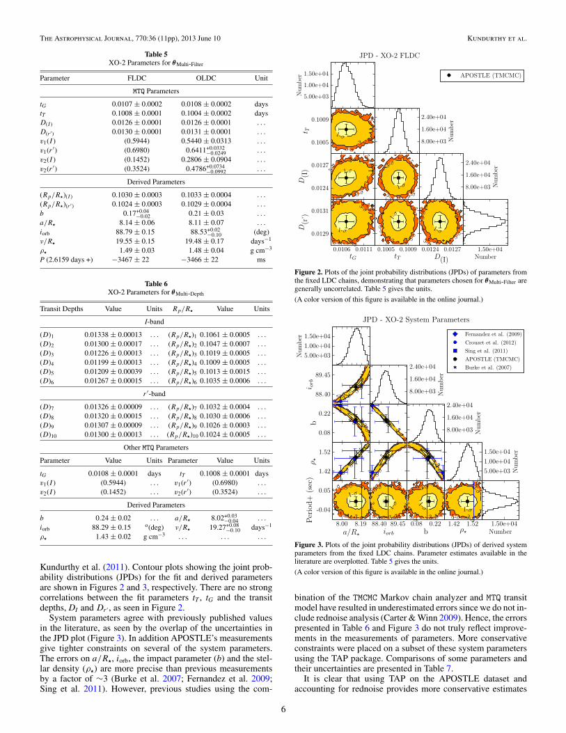
Kundurthy et al. (2011). Contour plots showing the joint prob-ability distributions (JPDs) for the fit and derived parametersare shown in Figures 2 and 3, respectively. There are no strongcorrelations between the fit parameters tT , tG and the transitdepths, DI and Dr ′ , as seen in Figure 2.

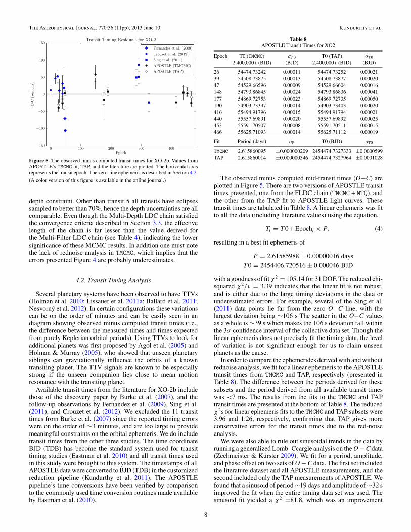
System parameters agree with previously published valuesin the literature, as seen by the overlap of the uncertainties inthe JPD plot (Figure 3). In addition APOSTLE’s measurementsgive tighter constraints on several of the system parameters.The errors on a/R�, iorb, the impact parameter (b) and the stel-lar density (ρ�) are more precise than previous measurementsby a factor of ∼3 (Burke et al. 2007; Fernandez et al. 2009;Sing et al. 2011). However, previous studies using the com-

Figure 2. Plots of the joint probability distributions (JPDs) of parameters fromthe fixed LDC chains, demonstrating that parameters chosen for θMulti-Filter aregenerally uncorrelated. Table 5 gives the units.

(A color version of this figure is available in the online journal.)

Figure 3. Plots of the joint probability distributions (JPDs) of derived systemparameters from the fixed LDC chains. Parameter estimates available in theliterature are overplotted. Table 5 gives the units.

(A color version of this figure is available in the online journal.)

bination of the TMCMC Markov chain analyzer and MTQ transitmodel have resulted in underestimated errors since we do not in-clude rednoise analysis (Carter & Winn 2009). Hence, the errorspresented in Table 6 and Figure 3 do not truly reflect improve-ments in the measurements of parameters. More conservativeconstraints were placed on a subset of these system parametersusing the TAP package. Comparisons of some parameters andtheir uncertainties are presented in Table 7.

It is clear that using TAP on the APOSTLE dataset andaccounting for rednoise provides more conservative estimates

6

The Astrophysical Journal, 770:36 (11pp), 2013 June 10 Kundurthy et al.

Figure 4. The transit depth D as a function of transit epoch for both I-band and r ′-band observations of XO-2b. The solid horizontal and dashed lines represent thebest-fit value and errors, respectively, for D from the fixed LDC TMCMC fit. The dotted line is the weighted mean of transit depth values from the Multi-Depth fixedLDC chains.

Table 7Comparison of Estimates of System Parameters for XO-2b

Parameter TMCMC TAP B07 F09 S11 C12 Units

a/R� 8.14 ± 0.06 8.13 ± 0.10 8.20 ± 0.20 8.13 ± 0.20 7.83 ± 0.17 7.99 ± 0.07 . . .

iorb 88.79 ± 0.15 88.80 ± 0.61 88.90 ± 0.75 . . . 87.62 ± 0.51 88.01 ± 0.33 (deg)b 0.172+0.040

−0.021 0.171 ± 0.085 0.158 ± 0.110 0.160 ± 0.110 0.324 ± 0.070 0.280 ± 0.044 . . .

ρ� 1.49 ± 0.03 1.49 ± 0.05 1.52 ± 0.11 1.48 ± 0.10 1.33 ± 0.09 1.41 ± 0.04 g cm−3

Notes. TMCMC and TAP values are from independent analysis of APOSTLE light curves; B07: Burke et al. 2007; F09: Fernandez et al.2009; S11: Sing et al. 2011; C12: Crouzet et al. 2012.

of the system parameters when compared to TMCMC values. TAPerrors for a/R� and ρ� are better than those reported by Sing et al.(2011) by up to ∼40%, whose observations were made usingthe 10.4 m Gran Telescopio Canarias (GTC). One must notethe Sing et al. (2011) data result from narrow-band photometryand hence would have much lower photometric precision whencompared to broadband observations from the same telescope.The resulting TAP errors for the impact parameter (b) and theorbital inclination are larger than those from the GTC studyby ∼20%. Thus we report only some improvements in themeasurements of system parameters. Our system parametersagree with the current best estimates reported in Crouzet et al.(2012), but our error bars are larger by factors �2.

4.1. Transit Depth Analysis

Figure 4 shows transit depth versus transit epoch for theI-band (top panel) and r ′-band (bottom panel). The overallvariations in the I-band depth are ∼0.05% compared to the0.01% uncertainty in D(I ) from the joint fit to depths in the FLDCchain. Depth variations can be caused by spots. Even though thevariations we present are significant we refrain from claimingthe detection of spot-modulation. These deviations are likely due

to the incomplete sampling of several transits. Spots influencestellar brightness to a greater extent at shorter wavelengths,so the r ′-band would be more conducive to showing depthvariations. However, the overall depth variation in the r ′-bandlight curves is of the order of 0.01% and is consistent with theerrors on D(r ′) from the fit reported by the FLDC chain (Table 5).The variations seen in the I-band depths are difficult to explain.They can either be due to (1) real brightness variations causedby spot-modulations, or (2) variations arising from the transitmodel’s inability to accurately constrain transit depths and errorsgiven the incomplete sampling of light curves (like transits 4–6).We note that errors on the transit depth from our Multi-DepthLDC chains are more sensitive to the incompleteness of in-eclipse data rather than the photometric precision of a given lightcurve. For example, transit numbers 4 and 6 have 86% and 72%of the in-eclipse transit data sampled, respectively; they alsohave light curve residuals of 939 ppm and 405 ppm, respectively.Thus even though transit 6 has significantly better photometricprecision, the depth for transit 4 is constrained slightly betterdue to the fact that more in-eclipse points are available. Amore dramatic difference can be seen with transit 5, which hasonly 47% of the in-eclipse light curve sampled and the worst

7

The Astrophysical Journal, 770:36 (11pp), 2013 June 10 Kundurthy et al.

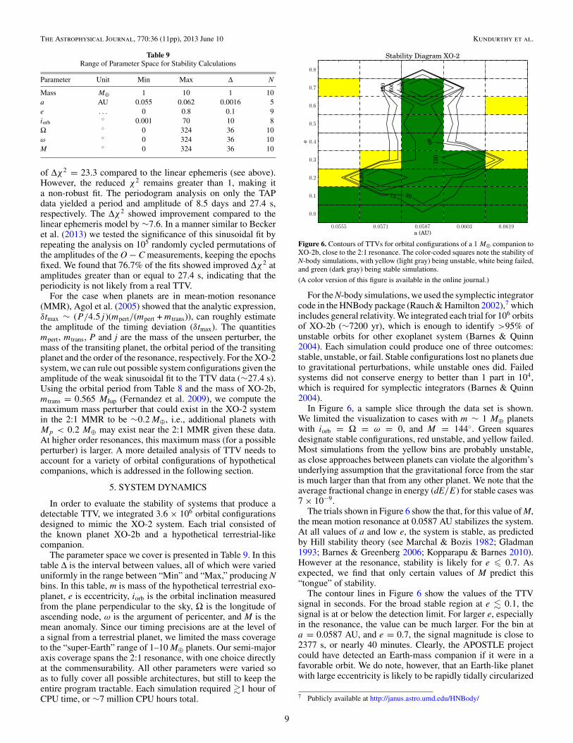
Figure 5. The observed minus computed transit times for XO-2b. Values fromAPOSTLE’s TMCMC fit, TAP, and the literature are plotted. The horizontal axisrepresents the transit epoch. The zero-line ephemeris is described in Section 4.2.

(A color version of this figure is available in the online journal.)

depth constraint. Other than transit 5 all transits have eclipsessampled to better than 70%, hence the depth uncertainties are allcomparable. Even though the Multi-Depth LDC chain satisfiedthe convergence criteria described in Section 3.3, the effectivelength of the chain is far lesser than the value derived forthe Multi-Filter LDC chain (see Table 4), indicating the lowersignificance of these MCMC results. In addition one must notethe lack of rednoise analysis in TMCMC, which implies that theerrors presented Figure 4 are probably underestimates.

4.2. Transit Timing Analysis

Several planetary systems have been observed to have TTVs(Holman et al. 2010; Lissauer et al. 2011a; Ballard et al. 2011;Nesvorny et al. 2012). In certain configurations these variationscan be on the order of minutes and can be easily seen in andiagram showing observed minus computed transit times (i.e.,the difference between the measured times and times expectedfrom purely Keplerian orbital periods). Using TTVs to look foradditional planets was first proposed by Agol et al. (2005) andHolman & Murray (2005), who showed that unseen planetarysiblings can gravitationally influence the orbits of a knowntransiting planet. The TTV signals are known to be especiallystrong if the unseen companion lies close to mean motionresonance with the transiting planet.

Available transit times from the literature for XO-2b includethose of the discovery paper by Burke et al. (2007), and thefollow-up observations by Fernandez et al. (2009), Sing et al.(2011), and Crouzet et al. (2012). We excluded the 11 transittimes from Burke et al. (2007) since the reported timing errorswere on the order of ∼3 minutes, and are too large to providemeaningful constraints on the orbital ephemeris. We do includetransit times from the other three studies. The time coordinateBJD (TDB) has become the standard system used for transittiming studies (Eastman et al. 2010) and all transit times usedin this study were brought to this system. The timestamps of allAPOSTLE data were converted to BJD (TDB) in the customizedreduction pipeline (Kundurthy et al. 2011). The APOSTLEpipeline’s time conversions have been verified by comparisonto the commonly used time conversion routines made availableby Eastman et al. (2010).

Table 8APOSTLE Transit Times for XO2

Epoch T0 (TMCMC) σT 0 T0 (TAP) σT 0

2,400,000+ (BJD) (BJD) 2,400,000+ (BJD) (BJD)

26 54474.73242 0.00011 54474.73252 0.0002139 54508.73875 0.00013 54508.73877 0.0002047 54529.66596 0.00009 54529.66604 0.00016148 54793.86845 0.00024 54793.86836 0.00041177 54869.72753 0.00023 54869.72735 0.00050190 54903.73397 0.00014 54903.73403 0.00020416 55494.91796 0.00015 55494.91794 0.00021440 55557.69891 0.00020 55557.69892 0.00025453 55591.70507 0.00008 55591.70511 0.00015466 55625.71093 0.00014 55625.71112 0.00019

Fit Period (days) σP T0 (BJD) σT0

TMCMC 2.615860095 ±0.000000209 2454474.7327333 ±0.0000599TAP 2.615860014 ±0.000000346 2454474.7327964 ±0.0001028

The observed minus computed mid-transit times (O−C) areplotted in Figure 5. There are two versions of APOSTLE transittimes presented, one from the FLDC chain (TMCMC + MTQ), andthe other from the TAP fit to APOSTLE light curves. Thesetransit times are tabulated in Table 8. A linear ephemeris was fitto all the data (including literature values) using the equation,

Ti = T 0 + Epochi × P, (4)

resulting in a best fit ephemeris of

P = 2.61585988 ± 0.00000016 days

T 0 = 2454406.720516 ± 0.000046 BJD

with a goodness of fit χ2 = 105.14 for 31 DOF. The reduced chi-squared χ2/ν = 3.39 indicates that the linear fit is not robust,and is either due to the large timing deviations in the data orunderestimated errors. For example, several of the Sing et al.(2011) data points lie far from the zero O−C line, with thelargest deviation being ∼106 s The scatter in the O−C valuesas a whole is ∼39 s which makes the 106 s deviation fall withinthe 3σ confidence interval of the collective data set. Though thelinear ephemeris does not precisely fit the timing data, the levelof variation is not significant enough for us to claim unseenplanets as the cause.

In order to compare the ephemerides derived with and withoutrednoise analysis, we fit for a linear ephemeris to the APOSTLEtransit times from TMCMC and TAP, respectively (presented inTable 8). The difference between the periods derived for thesesubsets and the period derived from all available transit timeswas <7 ms. The results from the fits to the TMCMC and TAPtransit times are presented at the bottom of Table 8. The reducedχ2s for linear ephemeris fits to the TMCMC and TAP subsets were3.96 and 1.26, respectively, confirming that TAP gives moreconservative errors for the transit times due to the red-noiseanalysis.

We were also able to rule out sinusoidal trends in the data byrunning a generalized Lomb–Ccargle analysis on the O − C data(Zechmeister & Kurster 2009). We fit for a period, amplitude,and phase offset on two sets of O − C data. The first set includedthe literature dataset and all APOSTLE measurements, and thesecond included only the TAP measurements of APOSTLE. Wefound that a sinusoid of period ∼19 days and amplitude of ∼32 simproved the fit when the entire timing data set was used. Thesinusoid fit yielded a χ2 =81.8, which was an improvement

8

The Astrophysical Journal, 770:36 (11pp), 2013 June 10 Kundurthy et al.

Table 9Range of Parameter Space for Stability Calculations

Parameter Unit Min Max Δ N

Mass M⊕ 1 10 1 10a AU 0.055 0.062 0.0016 5e . . . 0 0.8 0.1 9iorb

◦ 0.001 70 10 8Ω ◦ 0 324 36 10ω ◦ 0 324 36 10M ◦ 0 324 36 10

of Δχ2 = 23.3 compared to the linear ephemeris (see above).However, the reduced χ2 remains greater than 1, making ita non-robust fit. The periodogram analysis on only the TAPdata yielded a period and amplitude of 8.5 days and 27.4 s,respectively. The Δχ2 showed improvement compared to thelinear ephemeris model by ∼7.6. In a manner similar to Beckeret al. (2013) we tested the significance of this sinusoidal fit byrepeating the analysis on 105 randomly cycled permutations ofthe amplitudes of the O − C measurements, keeping the epochsfixed. We found that 76.7% of the fits showed improved Δχ2 atamplitudes greater than or equal to 27.4 s, indicating that theperiodicity is not likely from a real TTV.

For the case when planets are in mean-motion resonance(MMR), Agol et al. (2005) showed that the analytic expression,δtmax ∼ (P/4.5j )(mpert/(mpert + mtrans)), can roughly estimatethe amplitude of the timing deviation (δtmax). The quantitiesmpert, mtrans, P and j are the mass of the unseen perturber, themass of the transiting planet, the orbital period of the transitingplanet and the order of the resonance, respectively. For the XO-2system, we can rule out possible system configurations given theamplitude of the weak sinusoidal fit to the TTV data (∼27.4 s).Using the orbital period from Table 8 and the mass of XO-2b,mtrans = 0.565 MJup (Fernandez et al. 2009), we compute themaximum mass perturber that could exist in the XO-2 systemin the 2:1 MMR to be ∼0.2 M⊕, i.e., additional planets withMp < 0.2 M⊕ may exist near the 2:1 MMR given these data.At higher order resonances, this maximum mass (for a possibleperturber) is larger. A more detailed analysis of TTV needs toaccount for a variety of orbital configurations of hypotheticalcompanions, which is addressed in the following section.

5. SYSTEM DYNAMICS

In order to evaluate the stability of systems that produce adetectable TTV, we integrated 3.6 × 106 orbital configurationsdesigned to mimic the XO-2 system. Each trial consisted ofthe known planet XO-2b and a hypothetical terrestrial-likecompanion.

The parameter space we cover is presented in Table 9. In thistable Δ is the interval between values, all of which were varieduniformly in the range between “Min” and “Max,” producing Nbins. In this table, m is mass of the hypothetical terrestrial exo-planet, e is eccentricity, iorb is the orbital inclination measuredfrom the plane perpendicular to the sky, Ω is the longitude ofascending node, ω is the argument of pericenter, and M is themean anomaly. Since our timing precisions are at the level ofa signal from a terrestrial planet, we limited the mass coverageto the “super-Earth” range of 1–10 M⊕ planets. Our semi-majoraxis coverage spans the 2:1 resonance, with one choice directlyat the commensurability. All other parameters were varied soas to fully cover all possible architectures, but still to keep theentire program tractable. Each simulation required �1 hour ofCPU time, or ∼7 million CPU hours total.

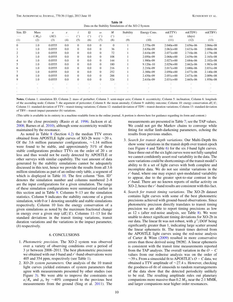
Figure 6. Contours of TTVs for orbital configurations of a 1 M⊕ companion toXO-2b, close to the 2:1 resonance. The color-coded squares note the stability ofN-body simulations, with yellow (light gray) being unstable, white being failed,and green (dark gray) being stable simulations.

(A color version of this figure is available in the online journal.)

For the N-body simulations, we used the symplectic integratorcode in the HNBody package (Rauch & Hamilton 2002),7 whichincludes general relativity. We integrated each trial for 106 orbitsof XO-2b (∼7200 yr), which is enough to identify >95% ofunstable orbits for other exoplanet system (Barnes & Quinn2004). Each simulation could produce one of three outcomes:stable, unstable, or fail. Stable configurations lost no planets dueto gravitational perturbations, while unstable ones did. Failedsystems did not conserve energy to better than 1 part in 104,which is required for symplectic integrators (Barnes & Quinn2004).

In Figure 6, a sample slice through the data set is shown.We limited the visualization to cases with m ∼ 1 M⊕ planetswith iorb = Ω = ω = 0, and M = 144◦. Green squaresdesignate stable configurations, red unstable, and yellow failed.Most simulations from the yellow bins are probably unstable,as close approaches between planets can violate the algorithm’sunderlying assumption that the gravitational force from the staris much larger than that from any other planet. We note that theaverage fractional change in energy (dE/E) for stable cases was7 × 10−9.

The trials shown in Figure 6 show the that, for this value of M,the mean motion resonance at 0.0587 AU stabilizes the system.At all values of a and low e, the system is stable, as predictedby Hill stability theory (see Marchal & Bozis 1982; Gladman1993; Barnes & Greenberg 2006; Kopparapu & Barnes 2010).However at the resonance, stability is likely for e � 0.7. Asexpected, we find that only certain values of M predict this“tongue” of stability.

The contour lines in Figure 6 show the values of the TTVsignal in seconds. For the broad stable region at e � 0.1, thesignal is at or below the detection limit. For larger e, especiallyin the resonance, the value can be much larger. For the bin ata = 0.0587 AU, and e = 0.7, the signal magnitude is close to2377 s, or nearly 40 minutes. Clearly, the APOSTLE projectcould have detected an Earth-mass companion if it were in afavorable orbit. We do note, however, that an Earth-like planetwith large eccentricity is likely to be rapidly tidally circularized

7 Publicly available at http://janus.astro.umd.edu/HNBody/

9

The Astrophysical Journal, 770:36 (11pp), 2013 June 10 Kundurthy et al.

Table 10Data on the Stability Simulations of the XO-2 System

Sim. ID Mass a e i Ω ω M Stability Energy Cons. std(TTV) std(TDV) std(TBV)· · · ( M⊕) (AU) · · · (◦) (◦) (◦) (◦) · · · · · · (s) (days) · · ·(1) (2) (3) (4) (5) (6) (7) (8) (9) (10) (11) (12) (13)

0 1.0 0.0555 0.0 0 0.0 0 0 1 2.370e-09 2.040e+00 2.656e-06 2.066e-081 1.0 0.0555 0.0 0 0.0 0 36 1 2.630e-09 2.062e+00 2.633e-06 2.000e-082 1.0 0.0555 0.0 0 0.0 0 72 1 2.610e-09 2.077e+00 2.710e-06 2.179e-083 1.0 0.0555 0.0 0 0.0 0 108 1 2.050e-09 2.068e+00 2.639e-06 2.165e-084 1.0 0.0555 0.0 0 0.0 0 144 1 1.980e-09 2.027e+00 2.684e-06 2.102e-085 1.0 0.0555 0.0 0 0.0 0 180 1 9.120e-10 2.029e+00 2.662e-06 1.983e-086 1.0 0.0555 0.0 0 0.0 0 216 1 2.210e-09 2.017e+00 2.680e-06 2.031e-087 1.0 0.0555 0.0 0 0.0 0 252 1 2.300e-09 2.050e+00 2.677e-06 2.140e-088 1.0 0.0555 0.0 0 0.0 0 288 1 2.430e-09 2.051e+00 2.673e-06 2.009e-089 1.0 0.0555 0.0 0 0.0 0 324 1 2.610e-09 2.031e+00 2.665e-06 1.958e-08. . . . . . . . . . . . .. . . . . . . . . . . . .. . . . . . . . . . . . .

Notes. Column 1: simulation ID; Column 2: mass of perturber; Column 3: semi-major axis; Column 4: eccentricity; Column 5: inclination; Column 6: longitudeof the ascending node; Column 7: the argument of pericenter; Column 8: the mean anomaly; Column 9: stability outcome; Column 10: energy conservation dE/E;Column 11: standard deviation of TTV—transit timing variations; Column 12: standard deviation of TDV—transit duration variations; Column 13: standard deviationof TBV—transit impact parameter (b) variations.

(This table is available in its entirety in a machine-readable form in the online journal. A portion is shown here for guidance regarding its form and content.)

due to the close proximity (Rasio et al. 1996; Jackson et al.2008; Barnes et al. 2010), although some eccentricity would bemaintained by the resonance.

As noted in Table 8 (Section 4.2) the median TTV errorsobtained from APOSTLE light curves of XO-2b were ∼20 s.Of the 3.6 million parameter configurations, ∼1.14 millionwere found to be stable, and approximately 51% of thesestable configurations produce TTVs on the order of 20 s orless and thus would not be easily detected by APOSTLE orother surveys with similar capability. The vast amount of datagenerated by the stability simulations cannot be adequatelydiscussed in this text, hence we provide the results from all 3.6million simulations as part of an online-only table, a segment ofwhich is displayed in Table 10. The first column “Sim. ID”denotes the simulation number and columns numbered 2–8are the input configurations for a given simulation. The rangeof these simulation configurations were summarized earlier inthis section and in Table 9. Columns 9–13 are the simulationstatistics. Column 9 indicates the stability outcome of a givensimulation, with 0 or 1 denoting unstable and stable simulationsrespectively. Column 10 lists the energy conservation of agiven simulations as noted by the maximum fractional changein energy over a given step (dE/E). Columns 11–13 list thestandard deviations in the transit timing variations, transitduration variations and the variations in the impact parameter,(b) respectively.

6. CONCLUSIONS

1. Photometric precision. The XO-2 system was observedover a variety of observing conditions over a period of3 yr between 2008–2011. The best photometric precisionswe obtained with our I-band and r ′-band observations were405 and 354 ppm, respectively (see Table 1).

2. XO-2b system parameters. Our analysis of the 10 transitlight curves yielded estimates of system parameters thatagree with measurements presented by other studies (seeFigure 3). We were able to improve the constraints ona/R� and ρ� by ∼40% compared to the previous bestmeasurements from the ground (Sing et al. 2011). The

measurements are presented in Table 7; see the TAP values.We could not get the Markov chains to converge whilefitting for stellar limb-darkening parameters, echoing theresults from previous studies.

3. Search for transit depth variations. Our Multi-Depth fitsshow some variations in the transit depth over transit epoch(see Figure 4 and Table 6) for the six I-band light curves.Since three out of the six light curves were not fully sampledwe cannot confidently assert real variability in the data. Theseen variations could be shortcomings of the transit model’sability to fit a set of light curves with both complete andincomplete data. We do not see similar variations in ther ′-band, where one may expect spot-modulated variabilityto appear, due to the greater spot-to-star contrast in ther ′-band. There are no known reports of stellar activity onXO-2, hence the r ′-band results are consistent with this fact.

4. Search for transit timing variations. The XO-2b datasetcontains light curves with some of the best photometricprecisions achieved with ground-based observations. Sincephotometric precision directly translates to transit timingprecision we are able to report timing precisions as lowas 12 s (after red-noise analysis, see Table 8). We wereunable to detect significant timing deviations for XO-2b inour data. The linear fit was not robust, with χ2/DOF beingsignificantly greater than 1, indicating large scatter aroundthe linear ephemeris fit. The transit times derived fromthe APOSTLE light curves using the red-noise analysisof Carter & Winn (2009) resulted in more conservativeerrors than those derived using TMCMC. A linear ephemerisis consistent with the transit time measurements reportedfrom the TAP analysis. The overall variation in the O − Cvalues from our rednoise analysis was on the order of∼39 s. From a sinusoidal fit to APOSTLE’s O − C data, weobtained a TTV amplitude of ∼27.4 s. However, checkingthe goodness-of-fit of sinusoids to random rearrangementsof the data show that the detected periodicity unlikelyto be real. The resulting amplitude rules out planetarycompanions more massive than 0.2 M⊕ near the 2:1 MMR,and larger companions near higher order resonances.

10

The Astrophysical Journal, 770:36 (11pp), 2013 June 10 Kundurthy et al.

We conclude that the set of transit times published in theliterature for XO-2b and other transiting systems in generalare not suited for transit timing analysis. Lacking red-noiseanalysis leads to underestimated timing errors and maylead to premature reporting of timing variations. A properanalysis of transit times would need a simultaneous analysisof transit light curves using a transit model which is (1)suited for Bayesian inference (i.e., with a fairly uncorrelatedparameter set; Carter et al. 2008) and (2) a transit modelwhich can adequately account for red-noise in the data (likeTAP; Gazak et al. 2012). Using large data sets of transit lightcurves may be inefficient due to the slowness of Markovchains with the addition of model parameters. In addition tothe development of more detailed models, the utilization offast Markov chain algorithms (for e.g., Foreman-Mackeyet al. 2013) is also recommended.Our lack of detection of TTVs in the data for the Hot-JupiterXO-2b is also consistent with Kepler’s findings that (1)Hot-Jupiters tend to lack other planetary siblings (Lathamet al. 2011; Steffen et al. 2012) and (2) members of multi-planet systems with short period planets (Period <10 days)are more likely to be Hot-Neptunes (Latham et al. 2011;Lissauer et al. 2011b).

5. Dynamical study. We ran 3.6 million N-body simulations ofpossible multi-planet configurations near the 2:1 resonancein order to test for (1) orbital stability and (2) detectability ofTTV signals. We varied several properties of the hypothet-ical companion to XO-2b (see Table 9), to look for patternsin the resulting stability and transit times of the simulationsover parameter space. Of the several stable configurations,we find that ∼51% of the simulations would display TTVsweaker than the precision limits of our survey and hence re-main undetectable. The entire table of simulation statisticsare presented online (see Table 10).

Funding for this work came from NASA Origins grantNNX09AB32G and NSF Career grant 0645416. R.B. acknowl-edges funding from NASA Astrobiology Institute’s VirtualPlanetary Laboratory lead team, supported by NASA under co-operative agreement No. NNH05ZDA001C. Data presented inthis work are based on observations obtained with the ApachePoint Observatory 3.5 m telescope, which is owned and oper-ated by the Astrophysical Research Consortium. We also thankan anonymous referee for giving several helpful suggestions toimprove our paper. We thank the APO Staff, APO Engineers,Anjum Mukadam, and Russel Owen for helping the APOSTLEprogram with its observations and instrument characterization.We thank S. L. Hawley for scheduling our observations on APO.This work acknowledges the use of parts of J. Eastman’s EX-OFAST transit code as part of APOSTLE’s transit model MTQ.We also acknowledge the use of the PyAstronomy package.8

REFERENCES

Agol, E., Steffen, J., Sari, R., & Clarkson, W. 2005, MNRAS, 359, 567Ballard, S., Fabrycky, D., Fressin, F., et al. 2011, ApJ, 743, 200Barnes, R., & Greenberg, R. 2006, ApJL, 647, L163

8 http://www.hs.uni-hamburg.de/DE/Ins/Per/Czesla/PyA/PyA/index.html

Barnes, R., & Quinn, T. 2004, ApJ, 611, 494Barnes, R., Raymond, S. N., Greenberg, R., Jackson, B., & Kaib, N. A.

2010, ApJL, 709, L95Becker, A. C., Kundurthy, P., Agol, E., et al. 2013, ApJL, 764, L17Bertin, E., & Arnouts, S. 1996, A&AS, 117, 393Bessell, M. S. 1990, PASP, 102, 1181Brown, T. M., Charbonneau, D., Gilliland, R. L., Noyes, R. W., & Burrows, A.

2001, ApJ, 552, 699Burke, C. J., McCullough, P. R., Valenti, J. A., et al. 2007, ApJ, 671, 2115Burrows, A., Hubeny, I., Budaj, J., Knutson, H. A., & Charbonneau, D.

2007, ApJL, 668, L171Carter, J. A., & Winn, J. N. 2009, ApJ, 704, 51Carter, J. A., Yee, J. C., Eastman, J., Gaudi, B. S., & Winn, J. N. 2008, ApJ,

689, 499Charbonneau, D., Brown, T. M., Latham, D. W., & Mayor, M. 2000, ApJL,

529, L45Claret, A., & Bloemen, S. 2011, A&A, 529, A75Collier Cameron, A., Wilson, D. M., West, R. G., et al. 2007, MNRAS,

380, 1230Cousins, A. W. J. 1976, MNSSA, 35, 70Crouzet, N., McCullough, P. R., Burke, C., & Long, D. 2012, ApJ, 761, 7Eastman, J., Gaudi, B. S., & Agol, E. 2013, PASP, 125, 83Eastman, J., Siverd, R., & Gaudi, B. S. 2010, PASP, 122, 935Fernandez, J. M., Holman, M. J., Winn, J. N., et al. 2009, AJ, 137, 4911Ford, E. B. 2005, AJ, 129, 1706Foreman-Mackey, D., Hogg, D. W., Lang, D., & Goodman, J. 2013, PASP,

125, 306Fortney, J. J., Lodders, K., Marley, M. S., & Freedman, R. S. 2008, ApJ,

678, 1419Fukugita, M., Ichikawa, T., Gunn, J. E., et al. 1996, AJ, 111, 1748Gazak, J. Z., Johnson, J. A., Tonry, J., et al. 2012, AdAst, 2012, 697967Gelman, A., & Rubin, D. B. 1992, StaSc, 7, 457Gelman, A., Carlin, J. B., Stern, H. S., & Rubin, D. B. 2003, Bayesian Data

Analysis (2nd ed.; Boca Raton, FL: CRC Press)Gladman, B. 1993, Icar, 106, 247Haghighipour, N., & Kirste, S. 2011, CeMDA, 111, 267Holman, M. J., Fabrycky, D. C., Ragozzine, D., et al. 2010, Sci, 330, 51Holman, M. J., & Murray, N. W. 2005, Sci, 307, 1288Hubeny, I., Burrows, A., & Sudarsky, D. 2003, ApJ, 594, 1011Jackson, B., Greenberg, R., & Barnes, R. 2008, ApJ, 678, 1396Knutson, H. A., Charbonneau, D., Noyes, R. W., Brown, T. M., & Gilliland,

R. L. 2007, ApJ, 655, 564Knutson, H. A., Howard, A. W., & Isaacson, H. 2010, ApJ, 720, 1569Kopparapu, R. K., & Barnes, R. 2010, ApJ, 716, 1336Kundurthy, P., Agol, E., Becker, A. C., et al. 2011, ApJ, 731, 123Kundurthy, P., Becker, A. C., Agol, E., Barnes, R., & Williams, B. 2013, ApJ,

764, 8Latham, D. W., Rowe, J. F., Quinn, S. N., et al. 2011, ApJL, 732, L24Lissauer, J. J., Fabrycky, D. C., Ford, E. B., et al. 2011a, Natur, 470, 53Lissauer, J. J., Ragozzine, D., Fabrycky, D. C., et al. 2011b, ApJS, 197, 8Machalek, P., McCullough, P. R., Burke, C. J., et al. 2008, ApJ, 684, 1427Machalek, P., McCullough, P. R., Burrows, A., et al. 2009, ApJ, 701, 514Madhusudhan, N. 2012, ApJ, 758, 36Mandel, K., & Agol, E. 2002, ApJL, 580, L171Marchal, C., & Bozis, G. 1982, CeMec, 26, 311Monet, D. G., Levine, S. E., Canzian, B., et al. 2003, AJ, 125, 984Mukadam, A. S., Owen, R., Mannery, E., et al. 2011, PASP, 123, 1423Narita, N., Hirano, T., Sato, B., et al. 2011, PASJ, 63, L67Nesvorny, D., Kipping, D. M., Buchhave, L. A., et al. 2012, Sci, 336, 1133Rasio, F. A., Tout, C. A., Lubow, S. H., & Livio, M. 1996, ApJ, 470, 1187Rauch, K. P., & Hamilton, D. P. 2002, BAAS, 34, 938Roberts, G. O., & Rosenthal, J. S. 2009, J. Comput. Graph. Stat., 18, 349Sing, D. K., Desert, J.-M., Fortney, J. J., et al. 2011, A&A, 527, A73Southworth, J. 2010, MNRAS, 408, 1689Steffen, J. H., Ragozzine, D., Fabrycky, D. C., et al. 2012, PNAS, 109, 7982Tegmark, M., Strauss, M. A., Blanton, M. R., et al. 2004, PhRvD, 69, 103501Winn, J. N. 2011, in Exoplanets, ed. S. Seager (Tucson, AZ: Univ. Arizona

Press), 526Zechmeister, M., & Kurster, M. 2009, A&A, 496, 577

11