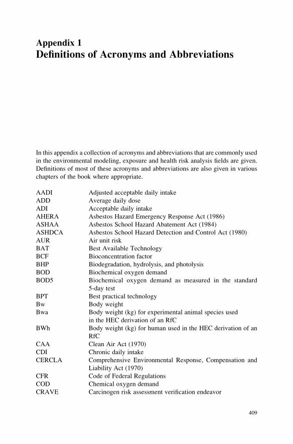
Appendix 1

Definitions of Acronyms and Abbreviations

In this appendix a collection of acronyms and abbreviations that are commonly used

in the environmental modeling, exposure and health risk analysis fields are given.

Definitions of most of these acronyms and abbreviations are also given in various

chapters of the book where appropriate.

AADI Adjusted acceptable daily intake

ADD Average daily dose

ADI Acceptable daily intake

AHERA Asbestos Hazard Emergency Response Act (1986)

ASHAA Asbestos School Hazard Abatement Act (1984)

ASHDCA Asbestos School Hazard Detection and Control Act (1980)

AUR Air unit risk

BAT Best Available Technology

BCF Bioconcentration factor

BHP Biodegradation, hydrolysis, and photolysis

BOD Biochemical oxygen demand

BOD5 Biochemical oxygen demand as measured in the standard

5-day test

BPT Best practical technology

Bw Body weight

Bwa Body weight (kg) for experimental animal species used

in the HEC derivation of an RfC

BWh Body weight (kg) for human used in the HEC derivation of an

RfC

CAA Clean Air Act (1970)

CDI Chronic daily intake

CERCLA Comprehensive Environmental Response, Compensation and

Liability Act (1970)

CFR Code of Federal Regulations

COD Chemical oxygen demand

CRAVE Carcinogen risk assessment verification endeavor

409

CSISSFRA Chemical Safety Information, Site Security and Fuels

Regulatory Relief Act (1999)

CWA Clean Water Act (1977)

CZMA Coastal Zone Management Act (1972)

DRA Dose–response assessment

DRR Dose response relationship

DW Drinking water

DWEL Drinking water equivalent level

EA Exposure assessment

EC Exposure concentration

EC50 Effective concentration, 50% affected

ED Effective dose

EED Estimated exposure dose

EMS Environmental management system

EMTD Estimated maximum tolerated dose

EP Extraction procedure

EPE Environmental performance evaluation

EPCRA Emergency Planning and Community Right-to-KnowAct (1986)

ESA Endangered Species Act (1973)

FEL Frank-effect level

FFDCA Federal Food, Drug, and Cosmetic Act (1938)

FIFRA Federal Insecticide, Fungicide and Rodenticide Act (1947)

FMEA Failure mode and effects analysis

FOIA The Freedom of Information Act (1966)

FQPA Food Quality Protection Act (1996)

FR Federal Register

HA Health Advisory

HAPPS Hazardous air pollution prioritization system

HAPs Hazardous air pollutants

HAS Health assessment summary

HAZOP Hazards and Operability Study

HDT Highest dose tested

HEAST Health effects assessment summary tables

HEC Human equivalent concentration

HEEP Health and environmental effects profile

HI Hazard index. Defined in terms of the ratio [intake/RfD], is

used to compare relative harmful noncarcinogenic effects

HMTA Hazardous Materials Transportation Act (1975)

HON Hazardous organic NESHAPs

HSDB Hazardous Substance Data Base

ICRP International Commission on Radiological Protection

IRAA Indoor Radon Abatement Act (1988)

IRIS Integrated risk information system

ISO International Organization for Standardization

410 Appendix 1 Definitions of Acronyms and Abbreviations

LADD Lifetime average daily dose

LBPPPA Lead-Based Paint Poisoning Prevention Act (1971)

LCA Life cycle assessment

LCCA Lead Contamination Control Act (1988)

LC50 Lethal concentration, 50% affected

LCLO Lethal concentration Low; the lowest concentration at which

death occurs

LC50 Lethal concentration 50; concentration lethal to 50% of the

animals

LD50 Lethal dose 50, dose lethal to 50% of the animals

LDL Lethal dose low – the lowest dose at which death occurs

LDT Lowest dose tested

LEL Lower explosive limit

LEL Lowest-effect level

LEPC Local Emergency Planning Committee

LOAEL Lowest observed adverse-effect level. A result of toxicological

studies which identify chemical concentration levels with criti-

cal toxic effect

LOAEL(ADJ) LOAEL adjusted to continuous exposure duration from an

intermittent regimen by hour/day and days/7 days

LOAEL(HEC) LOAEL adjusted for dosimetric differences across species to a

human equivalent concentration

LOC Limiting oxygen concentration

LOEL Lowest observed effect level

MACT Maximum Achievable Control Technology

MATC Maximum allowable toxicant concentration

MCL Maximum contaminant level

MCLG Maximum contaminant level goals

MEI Maximum exposed individual

MF Modifying factor

MOC Management of change

MOE Margin of exposure

MOS Margin of safety

MPRSA Marine Protection, Research, and Sanctuaries Act (1972)

MSDS Material Safety Data Sheet

MTBF Mean time between failure

MTD Maximum tolerated dose

MTL Median threshold limit

MTTF Mean time to failure

MWTA Medical Waste Tracking Act (1988)

NAAQS National Ambient Air Quality Standards

NEEA National Environmental Education Act (1990)

NEPA National Environmental Policy Act of 1969

NESHAP National Emission Standards for Hazardous Pollutants

Appendix 1 Definitions of Acronyms and Abbreviations 411

NOAEL No observed adverse-effect level. A result of toxicological stud-

ies which identify chemical concentration levels with no

observed toxic effect

NOAEL(ADJ) NOAEL adjusted to continuous exposure duration from an

intermittent regimen by hour/day and days/7 days

NOAEL(HEC) NOAEL adjusted for dosimetric differences across species to a

human equivalent concentration

NOEC No observed effects concentration

NOEL No observed effect level

NPDES National Pollutant Discharge Elimination System

NSPS New-Source Performance Standards

NTP National Toxicology Program

NWPA Nuclear Waste Policy Act (1982)

ODA Ocean Dumping Act (1972)

ODBA Ocean Dumping Ban Act (1988)

OHM/TADS Oil and Hazardous Materials Technical Assistance Data Systems

OPA The Oil Pollution Act of (1990)

OSHA The Occupational Safety and Health Act (1970)

P Probit dose extrapolation model

PBPK Physiologically based pharmacokinetic

PCi Picocurie

PD Position Document

PEL Permissible exposure limit

PELs Permissible exposure limits

PFD Process Flow Diagram

PHA Process hazards analysis

PMR Proportionate mortality ratio

PPA The Pollution Prevention Act (1990)

PPPA Pollution Prevention Packaging Act (1970)

PPE Personal protective equipment

PSA Process safety analysis

PSI Process safety information

PSM Process Safety Management

RA Risk assessment

RAFS Risk Assessment and Feasibility Study

RCRA Resource Conservation and Recovery Act

RDD Regional deposited dose

RDDR Regional deposited dose ratio used in derivation of an HEC for

particles

RDDR(ER) Regional deposited dose ratio used in the HEC derivation of an

RfC for an observed extrarespiratory effect of particles

RDDR(ET) Regional deposited dose ratio used in the HEC derivation of an

RfC for an observed effect of particles in the extrathoracic

region of the respiratory tract

412 Appendix 1 Definitions of Acronyms and Abbreviations

RDDR(PU) Regional deposited dose ratio used in the HEC derivation of an

RfC for an observed effect of particles in the pulmonary region

of the respiratory tract

RDDR(TB) Regional deposited dose ratio used in the HEC derivation of an

RfC for an observed effect of particles in the tracheobronchial

region of the respiratory tract

RDDR(TH) Regional deposited dose ratio used in the HEC derivation of an

RfC for an observed effect of particles in the thoracic region of

the respiratory tract

RDDR(TOTAL) Regional deposited dose ratio used in the HEC derivation of an

RfC for an observed effect of particles in the total respiratory

tract

RECRA Resource Conservation and Recovery Act

RGD Regional gas dose

RGDR Regional gas dose ratio used in the derivation of an HEC for

gases

RGDR(ET) Regional gas dose ratio used in the HEC derivation of an RfC

for an observed effect of a gas in the extrathoracic region of the

respiratory tract

RGDR(PU) Regional gas dose ratio used in the HEC derivation of an RfC

for an observed effect of a gas in the pulmonary region of the

respiratory tract

RGDR(TB) Regional gas dose ratio used in the HEC derivation of an RfC

for an observed effect of a gas in the tracheobronchial region of

the respiratory tract

RGDR(TH) Regional gas dose ratio used in the HEC derivation of an RfC

for an observed effect of a gas in the thoracic region of the

respiratory tract

RGDR(TOTAL) Regional gas dose ratio used in the HEC derivation of an RfC

for an observed effect of a gas in the total respiratory tract

RfD Reference dose

RfC Reference concentration

RgD Regulatory dose

RM Risk management

RME Reasonably maximally exposed individual

RMP Risk management plan

RQ Recordable quantity, reportable quantity

RRA Resource Recovery Act (1970)

RTECS Registry of Toxic Effects of Chemical Substances

RV Residual volume

Sa Surface area (in cm2) of respiratory tract region for experimen-

tal animal species used in the HEC derivation of an RfC

Sa(ET) Surface area (in cm2) of extrathoracic region for experimental

animal species used in the HEC derivation of an RfC

Appendix 1 Definitions of Acronyms and Abbreviations 413

Sa(TB) Surface area (in cm2) of tracheobronchial region for experimen-

tal animal species used in the HEC derivation of an RfC

Sa(TH) Surface area (in cm2) of thoracic region for experimental

animal species used in the HEC derivation of an RfC

Sa(PU) Surface area (in cm2) of pulmonary region for experimental

animal species used in the HEC derivation of an RfC

Sa(TOTAL) Surface area (in cm2) of total respiratory system for experimental

animal species used in the HEC derivation of an RfC

SAB Science Advisory Board

SANSS Structure and Nomenclature Search System

SAR Structure activity relationship

SARA Superfund Amendments and Reauthorization Act of 1986

SC Subcutaneous

SCE Sister-chromatid exchange

SDWA Safe Drinking Water Act (1974)

SECDA Shoreline Erosion Control Demonstration Act (1974)

SEPA Shoreline Erosion Protection Act (1965)

SF Slope factor, safety factor

Sh Surface area (in cm2) of respiratory tract for humans, used in

the HEC derivation of an RfC

Sh(ET) Surface area (in cm2) of extrathoracic region for humans, used

in the HEC derivation of an RfC

Sh(TB) Surface area (in cm2) of tracheobronchial region for humans,

used in the HEC derivation of an RfC

Sh(TH) Surface area (in cm2) of thoracic region for humans, used in the

HEC derivation of an RfC

Sh(PU) Surface area (in cm2) of pulmonary region for humans, used in

the HEC derivation of an RfC

Sh(TOTAL) Surface area (in cm2) of total respiratory system for humans,

used in the HEC derivation of an RfC

SIP State Implementation Plan

SMCL Secondary maximum contaminant level

SMCRA Surface Mining Control and Reclamation Act (1977)

SMR Standard mortality ratio

SPA Shore Protection Act (1988)

SPCC Spill Prevention Control and Countermeasures

STEL Short-term exposure limit

SWDA Solid Waste Disposal Act (1965)

TAG Technical Advisory Group

TD Toxic dose

TDB Toxicology data base

TEA Total exposure analysis

TEC Total environmental characterization

TLV Threshold limit value

414 Appendix 1 Definitions of Acronyms and Abbreviations

TQ Threshold quantity

TOC Total organic carbon

TOTAL Total respiratory tract

TRE Total resource effectiveness

TSCA Toxic Substances Control Act (1976)

TSS Total suspended solids

TWA Time weighed average

UCL Upper confidence limit

UEL Upper explosive limit

UF Uncertainty factor

UMTRCA Uranium Mill-Tailings Radiation Control Act (1978)

Vaa Alveolar ventilation rate (m3/day) for experimental animal

species used in HEC derivation of an RfC

Vah Alveolar ventilation rate (m3/day) for human used in HEC

derivation of an RfC

VOC Volatile organic compound

v/v Volume for volume

WBC White blood cell(s)

WQC Water quality criteria

Appendix 1 Definitions of Acronyms and Abbreviations 415

Appendix 2

Environmental Modeling and Exposure

Analysis Terms

In this appendix a list of terms which are commonly used in the environmental

modeling, exposure and health risk analysis fields are given, along with their

definitions.

Environmental Pathways and Processes

Advection Transport by an imposed or ambient velocity field in any

of the three coordinate directions (longitudinal, lateral

and transverse), as in river, canal or coastal water veloc-

ity fields, or as in a Darcy velocity field in an aquifer or a

wind velocity in the atmosphere.

Absorption Diffusion of a chemical into solid particles by a sorption

process through the boundary of the solid particles. Due

to this process, the transport of chemicals may be slowed

(retarded) or the solid particles may behave as long term

(secondary) sources for these chemicals due to potential

dissolution of the chemical from the solid particles back

into the medium.

Adsorption Attachment of chemicals to a particle surface during

a sorption process. Due to this process, the transport of

chemicals may be slowed (retarded) or the solid particles

may behave as long term (secondary) sources for these

chemicals due to potential desorption of the chemical

from the solid particles back into the medium.

Aquifer A geologic formation which contains water and transmits

water under normal drainage conditions.

417

Aquiclude A geologic formation which contains water but does not

transmit water.

Aquifuge A geologic formation that neither contains water nor

transmits water.

Aquitard A geologic formation which contains water and transmits

water at low rates relative to the transmission rate of

aquifers.

Conduction Transfer of energy by the jostling motion of atoms

through direct contact between atoms.

Convection Transport induced by hydrostatic instability, such as

density or temperature differences in a lake, reservoir

or atmosphere.

Chemical reaction By definition, chemical reactions involve the formation or

breakage of chemical bonds between atoms of a chemical.

Chemical reactions may be described in terms of chemical

kinetics, which describe the rate at which a reaction takes

place or of chemical equilibrium, which describe the final

expected chemical composition in a control volume.

Confined aquifier An aquifer which is bounded by impervious geologic

formations both from above and below.

Decay Radioactive chemicals or chemicals in general may

undergo decay, which will reduce the concentration

levels of both dissolved and sorbed phases. The rate of

disappearance (decay) of a chemical is usually expressed

in terms of the half life of the chemical.

Decomposition The decomposition process is a chemical recycling pro-

cess, in which organic compounds are broken down into

their inorganic components (mineralization or reminer-

alization). The agents which affect this process are bac-

teria or fungi, often in association with worms, insects

and other organisms that aid the process by breaking up

the organic matter both chemically and mechanically.

Deposition The removal of airborne substances to available surfaces

that occurs as a result of gravitational settling and diffu-

sion, as well as electrophoresis and thermophoresis.

Detection limit The lowest concentration of a chemical that can reliably

be distinguished from a zero concentration.

Diffusion Random walk of an ensemble of particles from regions of

high concentration to regions of low concentration.

Dispersion Refers to the mixing process by which the pollutants

or natural substances are mixed within a water or air

column. Four processes may contribute to dispersion

(mixing) at different levels of contribution to the overall

mixing: molecular diffusion, turbulent diffusion, shear

418 Appendix 2 Environmental Modeling and Exposure Analysis Terms

mixing and mechanical mixing. The importance or the

level of contribution of these mixing processes to the

overall dispersion is media dependent. For example, tur-

bulent diffusion may not be important in subsurface

transport, or mechanical mixing may not be considered

in surface or air transport.

Flocculation In surface waters, although individual small particles

may remain suspended and be transported, they may

also aggregate into clumps. This aggregation process is

called flocculation.

Half life Half life of a chemical is defined in terms of the time it takes

to reduce its chemical activity (concentration) by half.

Hydrodynamic

mixing

A process that describes the combined effects of mole-

cular diffusion and mechanical mixing in groundwater

transport.

Infiltration The process of water moving into the soil either from the

ground surface or from a surface water body.

Molecular diffusion Mixing associated with random molecular motions based

on gradients of concentration. This process may be

described by Fick’s law. This classical diffusion equation

relates the diffusion flux to concentration gradients in

terms of a “molecular diffusion” coefficient which is

chemical specific.

Mechanical mixing Mixing associated with random scattering of particles

associated with heterogeneity and tortuosity of particle

pathways in subsurface environments. The mathematical

definition is analogous to molecular diffusion, as it con-

tains a dynamic dispersivity coefficient, which is usually

expressed in terms of dispersion coefficient times the

average linear velocity, replacing the molecular diffusion

coefficients. Although it is media dependent, mechanical

mixing effects are usually much larger than molecular

diffusion effects in defining dispersion.

Percolation Water movement through the soil.

Retardation As a consequence of adsorptive and absorptive processes,

the transport of chemicals is slowed or retarded. In sub-

surface fate and transport modeling, the effect of this

process is introduced to the mathematical models in

terms of a retardation coefficient which is a function of

the ratio of the sorbed chemical concentration to the

mobile chemical concentration.

Runoff Water which is not absorbed by the soil or infiltrated to

the soil and flows to a lower ground, eventually draining

into a stream, river or other surface water bodies.

Appendix 2 Environmental Modeling and Exposure Analysis Terms 419

Sedimentation

(particle settling)

The sinking or rising of particles having densities differ-

ent from the ambient fluid, such as sand grains or organic

matter.

Semi-confined aquifier An aquifer bounded by a leaky aquifer from above or

below or both.

Solvent A liquid capable of dissolving or dispersing another

substance (for example, acetone or mineral spirits).

Sorption Chemicals in the environment may “sorb” onto the grains,

or onto iron oxyhydroxide, or organic coatings of grains of

aquifers or sediments in surface waters. The term “sorb”

includes both adsorptive and absorptive processes.

Suspension (particle

entrainment)

The picking up of particles, such as sand or organic

matter, from the bed of a water body by turbulent flow

past the bed.

Tributary A stream or river whose water flows into a larger stream

or river.

Turbulent diffusion The random scattering of particles by turbulent motion,

considered mainly in air and surface water pathways. Its

mathematical definition is analogous to molecular dif-

fusion, with “eddy” diffusion coefficient replacing the

molecular diffusion coefficients, which are much larger

than molecular diffusion coefficients.

Volatilization Transport mechanism associated with the transfer of

molecules from the liquid phase to the gas phase.

Volatile organic

compounds, VOCs

Organic compounds that evaporate readily into the air.

VOCs include substances such as benzene, toluene,

methylene chloride, and methyl chloroform.

Watershed The sum total all of the land and smaller surface water

bodies which drain into a stream or river at a point.

Water table aquifer An aquifer which is not bounded by another geologic

formation from above and the upper boundary is defined

in terms of a water level where the pressure condition is

atmospheric.

Environmental Modeling

Analytic solution A formula for the solution of a state variable in a mathe-

matical model that uses continuous and closed form

mathematical functions.

Analytic uncertainty Uncertainty associated with the individual parameters

used in defining a physical process in a model.

420 Appendix 2 Environmental Modeling and Exposure Analysis Terms

Analytic uncertainty

propagation

A procedure that examines how uncertainty in individual

parameters affects the overall uncertainty in model

predictions.

Boundary conditions Conditions on the primary unknowns (state variables) of

the problem posed, which must be satisfied at the bound-

aries of the solution domain.

Calibration A process that yields a model simulation output as close

as possible to the simulated event. The measure of cali-

bration is statistical comparisons between model results

and observations on the event. In a calibration process,

adjustment of model parameters within the range of

experimentally determined values reported in the litera-

ture or obtained through a site specific study is the key

operation. Calibration should not be confused with the

methods of parameter estimation.

Cauchy boundary

condition

A boundary condition in which the gradients of the

primary unknown variables (state variables) are defined

at the boundary of the solution domain, as a function of

the unknown variable. This boundary condition is also

referred to as the “third type” boundary condition.

Conservation

of energy

The energy associated with matter entering any system

plus the net energy added to the system is equal to the

energy leaving the system.

Conservation of mass Mass can neither be created nor destroyed, but can be

transferred or transformed. This law forms the basis of

most mechanistic models.

Conservation

of momentum

Momentum can neither be created nor destroyed, but can

be transferred or transformed. This law forms the basis of

Newton’s first law of motion.

Control volume Any closed reference volume across whose boundaries

one accounts for all transport fluxes, and within whose

boundaries one accounts for all processes that produce or

consume matter.

Descriptive statistics A branch of statistics that deals with the organization,

summarization, and presentation of data.

Difference equation A representation of a differential equation in terms of

discrete difference ratios that represents the derivatives

of the function and the value of the function at discrete

points.

Differential equation An equation involving a function and its derivatives.

Dirichlet

boundary condition

A boundary condition in which the value of the primary

unknown variables are defined at the boundary of the

solution domain. This boundary condition is also referred

to as the “first type” boundary condition.

Appendix 2 Environmental Modeling and Exposure Analysis Terms 421

Distribution A set of values derived from a specific population or set

of measurements that represents the range and array of

data for the factor being studied.

Initial condition A condition which defines the value and distribution of

the state variables at time zero or at the staring time of

the analysis.

Mass balance

(mass conservation)

An accounting process of mass inputs, outputs, reactions

and accumulation within a control volume.

Model A mathematical function with parameters which can be

adjusted so that the function closely describes a set of

empirical data. A “mathematical” or “mechanistic”

model is usually based on biological or physical mechan-

isms, and has model parameters that have real world

interpretation. In contrast, “statistical” or “empirical”

models curve-fit to data in which the mathematical func-

tion used is selected for its numerical properties. Extrap-

olation from mechanistic models (e.g., pharmacokinetic

equations) usually carries higher confidence than extrap-

olation using empirical models.

Mathematical model Representation of a chemical, physical or biological pro-

cess using mathematical principles.

Model inputs Forcing functions such as boundary or initial conditions,

or other parameters that characterize the process mod-

eled and are required to run a model.

Model parameters Coefficients used in a model to describe the process that

is modeled (e.g., rate coefficients, equilibrium coeffi-

cients).

Monte Carlo method A repeated random sampling from the distribution of

values for each of the parameters in a generic equation

(a model) representing a process, whose purpose is to

derive and estimate from the distribution of predictions

which is based on the generic equation.

Neuman

boundary condition

A boundary condition in which the gradients of

the primary unknown variables are defined at the

boundary of the solution domain. This boundary condi-

tion is also referred to as the “second type” boundary

condition.

Non-point source Distributed sources of contamination that may origi-

nate from runoff or percolation from land as a result of

different land use activities. In this case, while the flux

or load from a small area of the watershed may

be low, the overall loading to the watershed may be

large if the total area contributing to contamination is

large.

422 Appendix 2 Environmental Modeling and Exposure Analysis Terms

Numerical solution Use of a discrete (approximate) representation for the

solution of a state variable in a mathematical model.

Parameter estimation Usually identified as inverse solution in which the inde-

pendent variables of the models are treated as unknowns

and the dependent variables are treated as known

variables. This method yields the best estimates for the

parameters of the model based on data from dependent

variables.

Physiologically based

pharmacokinetic

model

Physiologically based compartmental model that is

used to describe (quantitatively) the pharmacokinetic

behavior of toxicants.

Point source Contaminants discharged to air, groundwater or surface

water from a defined source.

Population In statistical terms, it is used to define the collection of

measurements on all elements of a universe about which

one wishes to draw conclusions or make decisions.

Post audit Comparison of model results with field data that is

collected after the model is developed.

Probability analysis A field devoted to the study of random variation in

systems.

Probabilistic

uncertainty analysis

A technique that assigns a probability density func-

tion to each input parameter associated with a generic

equation (a model) representing a process, then ran-

domly selects values from each of the distributions

and inserts them into the generic equation. Repeated

calculations produce a distribution of predicted values

by the generic equation, which reflect the combined

impact of the variability in each input to the prediction.

Monte Carlo analysis is a common type of probabilistic

uncertainty analysis.

Random samples Samples selected from a statistical population such that

each sample has an equal probability of being selected.

Robust A statistical term which indicates that an association

between two variables remains significant when other

variables are taken into account.

Robustness Confidence in model results and applicability of the model

to represent the process that is modeled. Robustness is

established after repeated applications of the model simu-

late an event under different circumstances.

Sample A small part of something designed to show the nature or

quality of the whole.

Sensitivity analysis Process of changing one variable while leaving the other

variables in a model constant to determine the effect of

the changed variable on the output. In this procedure, the

Appendix 2 Environmental Modeling and Exposure Analysis Terms 423

uncertain quantity is selected at its credible lower and

upper bounds, while holding all others at their nominal

values, and the results are calculated at each combination

of values. The results may identify the variables that have

the greatest effect on predictions based on the generic

equation (model) and may help focus further attention on

specific aspects of data collection efforts.

Simulation The use of a model to produce information on state vari-

able(s) with any input data.

State variable The dependent variable of the model.

Statistical model A model based on random variables.

Steady state models Models in which the simulated value of the state variable

does not change with time.

Stochastic models Models that seek to identify and predict the probability

of occurrence of a given outcome in a process being

modeled.

Time dependent

models

Models in which the simulated value of the state variable

changes with time.

Uncertainty Uncertainty represents a lack of knowledge about factors

that affect the development of a representation of a pro-

cess or that could yield biased or inaccurate estimates

of the predicted value based on this representation. Thus

types of uncertainty may include uncertainty in a scenario,

in the parameters used in a model or in the model itself.

Uncertainty analysis Determination of the statistical uncertainty associated

with a state variable, due to uncertainty in model param-

eters, inputs, or the initial state through statistical or

stochastic methods.

Upper bound An estimate of the plausible upper limit to the true value

of the quantity. This is usually not a statistical confidence

limit.

Validation Scientific acceptance that: (i) the model includes all

major and salient processes of the system modeled

(ii) the processes are formulated correctly; and (iii) the

model properly describes the observed phenomena

within the physical, temporal and conceptual bound-

aries of its definition.

Variability Statistically represented range in the values of the para-

meters of a model or the values of the state variable.

Verification A statistically acceptable comparison between model

simulation results and a second set of independent data

on the process that is modeled. In the verification stage,

all calibrated model parameters are kept fixed at their

calibration values.

424 Appendix 2 Environmental Modeling and Exposure Analysis Terms

Environmental Toxicology

Acute exposure Exposure over a short period of time, usually in the range

of 24 h. may be used to define a single exposure or

multiple exposures during that period of time.

Acute toxicity Adverse effect that an organism experiences due to an

acute exposure. The older term used to describe immedi-

ate toxicty. Its former use was associated with toxic

effects that were severe (e.g., mortality) in contrast to

the term “subacute toxicity” that was associated with

toxic effects that were less severe. The term “acute toxi-

city” is often confused with that of acute exposure. The

examples of acute toxicity may range from a reaction to

an insect bite for very short term exposure to chemical

asphyxiation from exposure to high concentrations of

carbon monoxide (CO) for somewhat longer terms of

exposure.

Allergen A substance such as pollen or another protein to which a

subject becomes sensitized.

Allergic reaction A reaction to a toxicant caused by an altered state of the

normal immune response. The reaction can be defined in

terms of an immediate reaction such as the case of

anaphylaxis or delayed reaction such as the case in cell-

mediated reactions.

Anthropogenic An event which is a results of human activity, as opposed

to biogenic, which is a result of biologic activity.

Chronic exposure Exposure that is repeated over a longer period of time

(months).

Chronic toxicity Permanent adverse effect that an organism experiences

after exposure to a toxicant.

Dose The total amount of toxicant administered to an organism

within a specific time period. Units used to define this

term may depend on the application method, such as

quantity per unit body weight or quantity per unit body

surface area. Usually dose is a part of the total exposure

amount. Absorbed dose is the amount of a toxicant that

passes into a tissue or an organ.

Delayed or latent

toxicity

The adverse effect an organism experiences long after

the initiation of exposure to a toxicant.

Exposure The process by which an organism comes in contact with

a substance.

Exposure path The route of exposure for an organism to a substance,

such as air, water, soil, food, medication. The exposure

path usually resides in the ambient environment.

Appendix 2 Environmental Modeling and Exposure Analysis Terms 425

Idiosyncratic reaction A response to a toxicant which may occur at exposure

levels much lower than those that are required to cause

the same effect in the majority of individuals within the

same population.

Internal/absorbed dose The amount of toxicant that is absorbed into the organism

and distributed through systemic pathways.

In-vitro In an artificial environment outside a living organism or

body. For example, some toxicity testing is done on cell

cultures or slices of tissue grown in the laboratory, rather

than on a living animal

In-vivo Within a living organism or body. For example, some

toxicity testing is done on whole animals, such as rats

or mice

Local toxicity An adverse effect that is experienced at the toxicant’s site

of contact with an organism.

Mechanism of toxicity The biologic or biochemical processes through which a

toxicant’s effect on an organism is manifested.

Maximum

tolerated dose

The highest dose just below the level at which toxic

effects other than cancer can occur. Acute toxicity stud-

ies yield this dose level.

Reversible toxicity A reversible adverse effect that is experienced by an

organism to a toxic substance when the exposure is

terminated.

Safety A probabilistic measure of a specific exposure or dose

not producing a toxic effect.

Subacute exposure Similar to acute exposure, except that the exposure

period is longer. Usually exposure periods that ranges

from days to a month fall in this category.

Subchronic exposure Similar to chronic exposure in which the exposure period

is within several months.

Systemic toxicity An adverse effect that manifests itself at another point

of vulnerability distant from the point of entry of the

toxicant. The transfer processes from point of entry to

vulnerability point may include absorption, diffusion and

mechanical transfer. Examples would include the

adverse effects on the central nervous system resulting

from chronic ingestion of mercury.

Target organ dose The integral concentration of a toxicant in a target organ

that may cause health effects, over a time interval.

Teratogen A substance that causes defects in development between

conception and birth. A teratogen is a substance that

causes a structural or functional birth defect.

Toxic agent A substance that can have the characteristic of producing

an undesirable or an adverse health effect.

426 Appendix 2 Environmental Modeling and Exposure Analysis Terms

Toxin Any natural toxicant produced by an organism

Toxicant Any substance that causes adverse effects when in contact

with a living organism at a sufficiently high concentration.

Toxicity The adverse effect that a chemical or physical substance

might produce within a living organism.

Toxicology The science that is involved with the qualitative and

quantitative study of adverse health effects of chemicals

or physical substances which can be produced in living

organisms under specific conditions of exposure.

Exposure Analysis

Absorption fraction The relative amount of a substance that penetrates

through a surface into a body (unitless ratio).

Acceptable

daily intake

An estimate of the daily exposure dose that is likely to be

without deleterious effect even if continued exposure

occurs over a lifetime.

Acute exposure One dose or multiple doses occurring within a short time

(24 h or less).

Anecdotal data Data based on descriptions of individual cases rather than

on controlled studies.

Ambient The conditions surrounding a person, or the sampling

location.

Average daily dose Dose rate averaged over a pathway-specific period of

exposure expressed as a daily dose on a per-unit-body-

weight basis. The ADD, expressed in mass/mass-time

units, is used for exposure to chemicals with non-

carcinogenic non-chronic effects.

Best tracer method Method for estimating soil ingestion that allows for the

selection of the most recoverable tracer for a particular

subject or group of subjects. Selection of the best tracer is

made on the basis of the food/soil ratio.

Bioassay The determination of the potency (bioactivity) or con-

centration of a test substance by noting its effects in live

animals or in isolated organ preparations, as compared

with the effect of a standard preparation.

Bioavailability The degree to which a drug or other substance be-

comes available to the target tissue after administration

or exposure.

Carcinogen An agent capable of inducing a cancer response.

Carcinogenesis The origin or production of cancer, very likely a series of

steps. The carcinogenic event so modifies the genome and/

or other molecular control mechanisms in the target cells

that they can give rise to a population of altered cells.

Appendix 2 Environmental Modeling and Exposure Analysis Terms 427

Chronic effect An effect that is manifest after some time has elapsed

from initial exposure. See also Health hazard.

Chronic exposure Multiple exposures occurring over an extended period

of time, or a significant fraction of the animal’s or the

individual’s life-time.

Chronic intake The long term period over which a substance crosses

the outer boundary of an organism without passing an

absorption barrier.

Chronic study A toxicity study designed to measure the (toxic) effects

of chronic exposure to a chemical.

Chronic toxicity The older term used to describe delayed toxicity. How-

ever, the term “chronic toxicity” also refers to effects that

persist over a long period of time whether or not they

occur immediately or are delayed. The term “chronic

toxicity” is often confused with that of chronic exposure.

Confounder A condition or variable that may be a factor in producing

the same response as the agent under study. The effects

of such factors may be discerned through careful design

and analysis.

Core grade(s) Quality ratings, based on standard evaluation criteria

established by the Office of Pesticide Programs, given

to toxicological studies after submission by registrants.

Critical effect The first adverse effect, or its known precursor, that

occurs as the dose rate increases.

Developmental

toxicity

The study of adverse effects on the developing organism

(including death, structural abnormality, altered growth,

or functional deficiency) resulting from exposure prior to

conception (in either parent), during prenatal develop-

ment, or postnatally up to the time of sexual maturation.

Exposure Contact of a chemical, physical or biological agent

with the outer boundary of an organism. Exposure is

quantified as the concentration of the agent in the med-

ium in contact integrated over the time duration of the

contact.

Exposure assessment A process in which potential recipients (individual or

ecosystem) of a hazardous source are identified. This

includes, the magnitude of concentration levels, the dura-

tion, the frequency and the route of exposure.

Exposure

concentration

The concentration of a hazardous substance in its trans-

port or carrier medium at the point of contact.

Exposure duration The total time an individual or an ecosystem is exposed

to an hazardous substance.

Exposure pathway The physical path a chemical takes from the source of the

hazard to the exposure point.

428 Appendix 2 Environmental Modeling and Exposure Analysis Terms

Exposure registry A system of ongoing follow-up of people who have had

documented environmental exposures.

Exposure route Theway a chemical pollutant enters an organism after con-

tact, e.g., by ingestion, inhalation, or dermal absorption.

Exposure scenario A set of facts, assumptions, and inferences about how

exposure takes place that aids the exposure assessor in

evaluating, estimating, or quantifying exposures.

Endpoint A response measure in a toxicity study.

Estimated

exposure dose

(EED)

The measured or calculated dose to which humans are

likely to be exposed considering exposure by all sources

and routes.

Frank-effect

level (FEL)

Exposure level which produces unmistakable adverse

effects, such as irreversible functional impairment or

mortality, at a statistically or biologically significant

increase in frequency or severity between an exposed

population and its appropriate control.

Health advisory An estimate of acceptable drinking water levels for a

chemical substance based on health effects information;

a Health Advisory is not a legally enforceable Federal

standard, but serves as technical guidance to assist Fed-

eral, state, and local officials.

Immediate

versus delayed

toxicity

Immediate effects occur or develop rapidly after a single

administration of a substance, while delayed effects are

those that occur after the lapse of some time. These

effects have also been referred to as acute and chronic,

respectively.

Intake The process by which a substance crosses the outer

boundary of an organism without passing an absorption

barrier (e.g., through ingestion or inhalation).

Intake rate Rate of inhalation, ingestion, and dermal contact depend-

ing on the route of exposure.

Initiation The ability of an agent to induce a change in a tissue

which leads to the induction of tumors after a second

agent, called a promoter, is administered to the tissue

repeatedly.

Latency period The time between the initial induction of a health effect

and the manifestation (or detection) of the health effect;

crudely estimated as the time (or some fraction of the

time) from first exposure to detection of the effect.

Local versus systemic

toxicity

Local effects refer to those that occur at the site of first

contact between the biological system and the toxicant;

systemic effects are those that are elicited after absorp-

tion and distribution of the toxicant from its entry point to

a distant site.

Appendix 2 Environmental Modeling and Exposure Analysis Terms 429

Lowest-observed-

adverse-effect

level (LOAEL)

The lowest exposure level at which there are statistically

or biologically significant increases in frequency or sev-

erity of adverse effects between the exposed population

and its appropriate control group.

Malignant Tending to become progressively worse and to result in

death if not treated; having the properties of anaplasia,

invasiveness, and metastasis.

Margin of exposure

(MOE)

The ratio of the no observed adverse effect level

(NOAEL) to the estimated exposure dose (EED).

Margin of safety

(MOS)

The older term used to describe the margin of exposure.

Metastasis The transfer of disease from one organ or part to another

not directly connected with it adj., metastatic.

Microenvironment The combination of activities and locations that yield

potential exposure.

Modifying factor (MF) An uncertainty factor which is greater than zero and less

than or equal to 10; the magnitude of the MF depends

upon the professional assessment of scientific uncertain-

ties of the study and database not explicitly treated with

the standard uncertainty factors (e.g., the completeness

of the overall database and the number of species tested);

the default value for the MF is 1.

Morbidity The state of being ill or diseased. Morbidity is the occur-

rence of a disease or a condition that alters health and

quality of life.

Mortality Death. Usually the cause (a specific disease, a condition,

or an injury) is stated.

No evidence of

carcinogenicity

According to the U.S. EPA Guidelines for Carcinogen

Risk Assessment, a situation in which there is no

increased incidence of neoplasms in at least two well-

designed and well-conducted animal studies of adequate

power and dose in different species.

No-observed-adverse-

effect level

(NOAEL)

An exposure level at which there are no statistically or

biologically significant increases in the frequency or

severity of adverse effects between the exposed pop-

ulation and its appropriate control; effects may be pro-

duced at this level, but they are not considered as

adverse, nor precursors to adverse effects. In an experi-

ment with several NOAELs, the regulatory focus is

primarily on the highest one, leading to the common

usage of the term NOAEL as the highest exposure with-

out adverse effect.

No-observed-effect

level (NOEL)

An exposure level at which there are no statistically or

biologically significant increases in the frequency or

430 Appendix 2 Environmental Modeling and Exposure Analysis Terms

severity of any effect between the exposed population

and its appropriate control.

Occupational mobility An indicator of the frequency at which workers change

from one occupation to another.

Occupational tenure The cumulative number of years a person has worked in

his or her current occupation, regardless of the number of

employers, interruption in employment, or time spent in

other occupations.

Organoleptic Affecting or involving a sense organ as of taste, smell, or

sight.

Pathway The physical course that a chemical or pollutant takes

from the source to the organism exposed.

Per capita intake rate The average quantity of food consumed per person in a

population composed of both individuals who ate the

food during a specified period and those that did not.

Population mobility An indicator of the frequency at which individuals move

from one residential location to another.

Promoter In studies of skin cancer in mice, an agent which results in

an increase in cancer induction when administered after

the animal has been exposed to an initiator, which is

generally given at a dose which would not result in tumor

induction if given alone. A cocarcinogen differs from a

promoter in that it is administered at the same time as the

initiator. Cocarcinogens and promoters do not usually

induce tumors when administered separately. Complete

carcinogens act as both initiator and promoter. Some

known promoters also have weak tumorigenic activity,

and some also are initiators. Carcinogens may act as pro-

moters in some tissue sites and as initiators in others.

Proportionate

mortality ratio

(PMR)

The number of deaths from a specific cause and in a

specific period of time per 100 deaths in the same time

period.

Residential volume The volume of the structure in which an individual

resides and may be exposed to contaminants.

Residential occupancy

period

The time between when a person moves into a residence

and when the person moves out or dies.

Reportable quantity The quantity of a hazardous substance that is considered

reportable under CERCLA. Reportable quantities are: (1)

1 lb, or (2) for selected substances, an amount established

by regulation either under CERCLA or under Section 311

of the Clean Water Act. Quantities are measured over a

24-h period.

Reversible versus

irreversible toxicity

Reversible toxic effects are those that can be repaired,

usually by a specific tissue’s ability to regenerate or

Appendix 2 Environmental Modeling and Exposure Analysis Terms 431

mend itself after chemical exposure, while irreversible

toxic effects are those that cannot be repaired.

Route The way a chemical or pollutant enters an organism

after contact, e.g., by ingestion, inhalation, or dermal

absorption.

Safety factor See Uncertainty factor. Short-term exposure – multiple

or continuous exposures occurring over a week or so.

Screening level

assessment

Examination of exposures that would fall on or beyond

the high end of the expected exposure distribution.

Standardized mortality

ratio (SMR)

The ratio of observed deaths to expected deaths.

Subchronic exposure Multiple or continuous exposures occurring usually

over 3 months.

Subchronic study A toxicity study designed to measure effects from sub-

chronic exposure to a chemical.

Sufficient evidence According to the U.S. EPA’s Guidelines for Carcinogen

Risk Assessment, sufficient evidence is a collection of

facts and scientific references which is definitive enough

to establish that the adverse effect is caused by the agent

in question.

Superfund Federal authority that was established by the Compre-

hensive Environmental Response, Compensation, and

Liability Act (CERCLA) in 1980 to respond directly to

releases or threatened releases of hazardous substances

that may endanger health or welfare.

Supporting studies Those studies that contain information that is useful for

providing insight and support for conclusions.

Systemic effects Effects that require absorption and distribution of the

toxicant to a site distant from its entry point, at which

point effects are produced. Most chemicals that produce

systemic toxicity do not cause a similar degree of toxicity

in all organs, but usually demonstrate major toxicity to

one or two organs. These are referred to as the target

organs of toxicity for that chemical.

Systemic toxicity See Systemic effects.

Target organ of

toxicity

See Systemic effects.

Threshold The dose or exposure below which a significant adverse

effect is not expected. Carcinogens are thought to be non-

threshold chemicals, to which no exposure can be pre-

sumed to be without some risk of adverse effect.

Threshold limit values

(TLVs)

Recommended guidelines for occupational exposure to

airborne contaminants.

432 Appendix 2 Environmental Modeling and Exposure Analysis Terms

Total tap water Water consumed directly from the tap as a beverage

or used in the preparation of foods and beverages (i.e.,

coffee, tea, soups, etc.).

Total fluid intake Consumption of all types of fluids including tap water,

milk, soft drinks, alcoholic beverages and water intrinsic

to purchased foods.

Uncertainty factor One of several, generally tenfold factors, used to derive

operationally the reference dose (RfD) from experimental

data. UFs are intended to account for (1) the variation in

sensitivity among the members of the human population

(2) the uncertainty in extrapolating animal data to the case

of humans (3) the uncertainty in extrapolating from data

obtained in a study that is of less-than-lifetime exposure

and (4) the uncertainty in using LOAEL data rather than

NOAEL data.

Uptake The process by which a substance crosses an absorption

barrier and is absorbed into the body.

Weight-of-evidence

for carcinogenicity

The extent to which the available biomedical data sup-

port the hypothesis that a substance causes cancer in

humans.

Environmental Risk Analysis

Added risk The difference between the cancer incidence under the

exposure condition and the background incidence in the

absence of exposure.

Attributable risk The difference between the risk of exhibiting a certain

adverse effect in the presence of a toxic substance and

that risk in the absence of the substance.

Contaminant

concentration

The concentration of the contaminant in the medium

(air, water, soil, etc.). It has the units of mass/volume or

mass/mass.

Dose The amount of a substance available for interaction with

metabolic processes or biologically significant receptors

after crossing the outer boundary of an organism.

Dose–response

assessment

A process in which the quantity of a hazard that may

reach organs or tissues and the percentage of the exposed

populations are identified.

Dose–response

relationship

A relationship between the amount of an agent (either

administered, absorbed, or believed to be effective) and

changes in certain aspects of the biological system (usu-

ally toxic effects), apparently in response to that agent.

Appendix 2 Environmental Modeling and Exposure Analysis Terms 433

Excess lifetime risk The additional or extra risk incurred over the lifetime of

an individual by exposure to a toxic substance.

Extra risk The added risk to that portion of the population that is not

included in measurement of the background disease rate.

Hazard Hazard refers to the source of risk but is not synonymous

with risk. A chemical which is hazardous to human

health may not be considered to be a risk unless there

is an exposure pathway which links that chemical to

humans or to the environment.

Hazard control The process, through which one recognizes, evaluates

and eliminates the potential hazards of a hazardous

source.

Hazard identification Hazard identification is the first step in risk analysis,

which is the process of identifying all the hazards with

the potential to harm an individual or the environment.

Human equivalent

concentration

Exposure concentration for humans that has been

adjusted for dosimetric differences between experimen-

tal animal species and humans to be equivalent to the

exposure concentration associated with observed effects

in the experimental animal species. If occupational

human exposures are used for extrapolation, the human

equivalent concentration represents the equivalent

human exposure concentration adjusted to a continuous

basis.

Human equivalent

dose

The human dose of an agent that is believed to induce the

same magnitude of toxic effect as that which the known

animal dose has induced.

Incidence The number of new cases of a disease within a specified

period of time.

Incidence rate The ratio of the number of new cases over a period of

time to the population at risk.

Individual risk The probability that an individual person will experience

an adverse effect. This is identical to population risk

unless specific population subgroups can be identified

that have different (higher or lower) risks.

Inhaled dose The amount of an inhaled substance that is available for

interaction with metabolic processes or biologically sig-

nificant receptors after crossing the outer boundary of an

organism.

Internal dose

(absorbed dose)

The amount of substance penetrating across absorption

barriers of an organism, via either physical or biological

processes.

Interspecies dose

conversion

The process of extrapolating from animal doses to equiv-

alent human doses.

434 Appendix 2 Environmental Modeling and Exposure Analysis Terms

Lifetime average

daily dose

Dose averaged over a lifetime. LADD is used for

compounds with carcinogenic or chronic effects and

is expressed in terms of mg/kg-day or other mass/

mass-time units.

Limited evidence According to the U.S. EPA’s Guidelines for Carcinogen

Risk Assessment, limited evidence is a collection of facts

and accepted scientific inferences which suggest that the

agent may be causing an effect, but this suggestion is not

strong enough to be considered an established fact.

No data According to the U.S. EPA Guidelines for Carcinogen

Risk Assessment, “no data” describes a category of

human and animal evidence in which no studies are

available to permit one to draw conclusions as to the

induction of a carcinogenic effect.

Potential dose The amount of a chemical contained in material ingested,

air breathed, or bulk material applied to the skin.

Principal study The study that contributes most significantly to the quali-

tative and quantitative risk assessment.

Process hazard

analysis

An analysis conducted to identify, evaluate, eliminate or

control potential hazards within a plant of facility.

Prospective study A study in which subjects are followed forward in time

from initiation of the study. This is often called a longi-

tudinal or cohort study.

Reasonable risk Risk levels which may be considered tolerable. This level

may be determined through consensus building, by com-

paring costs, benefits and alternative risks that have pre-

viously been accepted as tolerable.

Reference

concentration (RfC)

An estimate (with uncertainty spanning perhaps an order

of magnitude) of a continuous inhalation exposure to the

human population (including sensitive subgroups) that is

likely to be without an appreciable risk of deleterious

noncancer effects during a lifetime.

Reference dose (RfD) An estimate (with uncertainty spanning perhaps an order

of magnitude) of a daily exposure to the human popula-

tion (including sensitive subgroups) that is likely to be

without an appreciable risk of deleterious effects during a

lifetime.

Regional deposited

dose (RDD)

The deposited dose of particles calculated for the region

of interest as related to the observed effect. For respira-

tory effects of particles, the deposited dose is adjusted for

ventilatory volumes and the surface area of the respira-

tory region effected (mg/min-cm2). For extrarespiratory

effects of particles, the deposited dose in the total respi-

ratory system is adjusted for ventilatory volumes and

body weight (mg/min-kg).

Appendix 2 Environmental Modeling and Exposure Analysis Terms 435

Regional deposited

dose ratio (RDDR)

The ratio of the regional deposited dose calculated for a

given exposure in the animal species of interest to the

regional deposited dose of the same exposure in a human.

This ratio is used to adjust the exposure effect level for

interspecies dosimetric differences to derive a human

equivalent concentration for particles.

Regional gas dose

(RGD)

The gas dose calculated for the region of interest as

related to the observed effect for respiratory effects.

The deposited dose is adjusted for ventilatory volumes

and the surface area of the respiratory region effected

(mg/min-cm2).

Regional gas dose

ratio (RGDR)

The ratio of the regional gas dose calculated for a given

exposure in the animal species of interest to the regional

gas dose of the same exposure in humans. This ratio is

used to adjust the exposure effect level for interspecies

dosimetric differences to derive a human equivalent con-

centration for gases with respiratory effects.

Regulatory dose (RgD) The daily exposure to the human population reflected in

the final risk management decision; it is entirely possible

and appropriate that a chemical with a specific RfD may

be regulated under different statutes and situations

through the use of different RgDs.

Relative risk

(sometimes referred

to as risk ratio)

The ratio of incidence or risk among exposed individuals

to incidence or risk among unexposed individuals.

Risk Risk is the probability of injury, disease, death or expo-

sure of individuals, populations or ecosystems which

creates a hazardous or adverse condition. In quantitative

terms, risk is expressed in values ranging from 0 (repre-

senting the certainty that harm will not occur) to 1

(representing the certainty that harm will occur). The

following are examples showing the manner in which

risk is expressed in IRIS: E-4¼ a risk of 1/10,000; E-5¼a risk of 1/100,000; E-6 ¼ a risk of 1/1,000,000. Simi-

larly, 1.3E-3 ¼ a risk of 1.3/1000 ¼ 1/770; 8E-3 ¼ a risk

of 1/125; and 1.2E-5 ¼ a risk of 1/83,000.

Risk assessment Risk assessment is a process in which the severity of

adverse effects imposed by a hazardous condition on a

population or an ecosystem is estimated.

Risk characterization A process in which a numerical value is associated with

the risk.

Risk communication The results of risk assessment and risk management must

be communicated to the technical and public communities

as the best alternative, based on the assumption and

436 Appendix 2 Environmental Modeling and Exposure Analysis Terms

limitations of the analysis performed. Communicating

these results is one of the most important aspects of the

overall risk analysis process, since the proposed action

plan has to have the support of the stake holders for it to

be successful.

Risk management Is the decision making process in which the results of the

risk assessment analysis are used to manage the risk in an

effort to reduce its overall effects on humans and ecosys-

tems.

Risk reduction Actions that can decrease the likelihood that individuals,

groups, or communities will experience disease or other

health conditions.

Slope factor The slope of the dose-response curve in the low-dose

region. When low-dose linearity cannot be assumed, the

slope factor is the slope of the straight line from 0 dose

(and 0 excess risk) to the dose at 1% excess risk. An

upper bound on this slope is usually used instead of the

slope itself. The units of the slope factor are usually

expressed as 1/(mg/kg-day).

Source assessment A process in which one identifies the source location, the

release history and the level of contaminant concentra-

tion released in that period.

Unit risk The upper-bound excess lifetime cancer risk estimated to

result from continuous exposure to an agent at a concen-

tration of 1 mg/L in water, or 1 mg/m3 in air.

Environmental Epidemiology

Biologic monitoring Measuring hazardous substances in biologic materials (such

as blood, hair, urine, or breath) to determine whether expo-

sure has occurred. A blood test for lead is an example of

biologic monitoring.

Body burden The total amount of a substance in the body. Some sub-

stances build up in the body because they are stored in fat or

bone or because they leave the body very slowly.

Case-control study An epidemiologic study that looks back in time at the

exposure history of individuals who have the health effect

(cases) and at a group who do not (controls), to ascertain

whether they differ in proportion exposed to the chemical

under investigation.

Cohort study An epidemiologic study that observes subjects in differently

exposed groups and compares the incidence of symptoms.

Appendix 2 Environmental Modeling and Exposure Analysis Terms 437

Although ordinarily prospective in nature, such a study is

sometimes carried out retrospectively, using historical data.

Confounding bias Bias that may not be avoided in both cohort and case-

control studies. For example, an evaluation of two variables

(exposure and disease) that is influenced by a third variable

that is also the cause of the disease and also associated with

exposure.

Control group A group of subjects observed in the absence of agent expo-

sure or, in the instance of a case/control study, in the

absence of an adverse response.

Observation bias Bias that occurs in an epidemiologic study due to deficien-

cies in the study design. In a cohort study, observation bias

may occur when information on disease outcome is

obtained in a non-comparable manner from exposed and

non-exposed groups. In case-control studies, observation

bias may occur when information on exposure is obtained

in a non-comparable manner from case controls.

Selection bias Bias that occurs in an epidemiologic study due to deficien-

cies in the study design. For example, if two groups of

persons, one exposed and the other not exposed to a toxi-

cant, are identified today and followed through time until

disease occurs, than no selection bias is possible. However,

if a group of people with disease is identified and a group of

controls is selected (case control study), selection bias is

possible since the disease had occurred prior to the initiation

of the study.

438 Appendix 2 Environmental Modeling and Exposure Analysis Terms

Appendix 3

Definitions and Operations of the ACTS/RISK

Software

The Analytical Contaminant Transport Analysis System (ACTS) software is a

computational platform designed to provide environmental engineers and health

scientists with a user friendly interface to access commonly used environmental

multimedia transformation and transport models for the four environmental path-

ways, i.e. air, soil, surface water, and groundwater pathways. The complementary

health risk analysis software (RISK) provides a computational platform to analyze

the health risk of exposure to contaminants that may be linked to the environmental

pathway analysis provided in ACTS, although it can also be used as an independent

application. ACTS and RISK contain more than 300 models that are available in the

public domain literature. The analytical solutions to these models are provided

under a unified computational platform and are accessed through an easy to learn

and easy to use graphical user interface. A powerful feature of both of these

computational platforms is their ability to conduct probabilistic analyses using

one- and two-stage Monte Carlo simulations that are dynamically linked to all

environmental pathway and risk analysis modules. Thus, third-party software is not

required to conduct Monte Carlo simulations in the ACTS and RISK applications.

Publication-quality graphical output of simulation results can be developed using

the graphic utilities included in the software.

Contributors to the ACTS/RISK Software

An application software that covers a wide range of environmental pathways and

exposure models that is developed in a user friendly interface necessarily requires

the contribution of numerous participants to the effort. In this case the participants

to the project are the former students of the author of this book. The author is

indebted to these contributors and would like to acknowledge their contributions by

including their names here in an alphabetical order: Dr. Jiabao Guan, Dr. Elcin

Kentel, Dr. Orhan Gunduz, Dr. Wasim Khan, Dr. Boshu Liao, Mr. Morris Maslia,

Ms. Jenny Morgan, Mr. William Morgan, Mr. Babar Sani.

439

The design of the ACTS/RISK software architecture is provided by Dr. Jiabao

Guan and Dr. Wasim Khan.

ACTS and RISK Software Download

The ACTS and RISK software has been updated several times over the years since

1993. These updates have been made to provide error free software as much as

possible. As this book goes into publication, we are now at Version 9 for ACTS and

Version 1 for RISK. The latest versions of these two software tools can be down-

loaded from the web addresses given below, free of charge.

http://mesl.ce.gatech.edu/SHARE/Share.html or http://extras.springer.com

Information on this can also be found on the home page of this volume on http://

www.springer.com

Disclaimer

Analytical models used in the ACTS and RISK software are available in the public

domain literature and have been used by the U. S. Geological Survey (USGS), U. S.

Environmental Protection Agency (EPA), U. S. Department of Health and Human

Services (DHHS) and other federal agencies, as well as private consulting compa-

nies and educational institutions. No warranty is expressed or implied by the author,

as to the accuracy and functioning of the programs and related material included in

the software tools that accompany this book. Nor shall the fact of distribution of the

ACTS and RISK software through the web page given above constitute any such

warranty, and no responsibility is assumed by the author for the use of this software

and the book in connection herewith. Any use of trade products, or company names

in this book is for descriptive purposes only and does not imply endorsement by the

author.

Background Information

In the development of the two computational platforms, a decision was made to

focus on four objectives:

l Developing a computational platform that would be easy to learn and easy to use

with a user-friendly graphical interfacel Inclusion of analytical models that focus on key parameters and their relation-

ship to exposure thresholds, which would allow users to make timely public

health decisions

440 Appendix 3 Definitions and Operations of the ACTS/RISK Software

l Developing an analysis system with the capability to conduct probabilistic

analyses to address issues of uncertainty and variability for all applications

included in the two software toolsl Ability to produce publication quality graphical output internally and also

provide text or spread sheet type output for use with external and third-party

applications if needed

To meet these objectives, the analytical contaminant transport analysis system

ACTS and health risk analysis system RISK was developed with partial funding

provided by the Agency for Toxic Substances and Disease Registry (ATSDR). The

resulting computational platform is in public domain and can be downloaded from

the Multimedia Environmental Simulations Laboratory (MESL) web page at the

Georgia Institute of Technology: http://mesl.ce.gatech.edu/SHARE/Share.html or

Springer web page: http://extras.springer.com

Overview of the Computational Platform

The ACTS and RISK software have been developed to provide professionals in

the fields of hydrogeology, environmental engineering, and environmental health

with compact analytical tools to evaluate the transformation and transport of

contaminants in multimedia environments such as air, soil, surface water, and

groundwater. ACTS and RISK were been initially released in 1993 and the most

current version is available over the Internet as described above. The transforma-

tion and transport models included in the software are dynamic models that can

be used to assess steady state and time dependent contaminant concentrations

introduced to soil layers or contaminants released into air or water (Fig. A3.1).

Transformation processes that can be simulated in ACTS include sorption, decay,

first-order biodegradation and multispecies by-product generation. Analysis of

the soil/air pathway within ACTS includes a chemical database, several emission

models are included for simulating the emission rates from a contaminated soil

layer to the land surface, and Box and Gaussian dispersion models are included

for evaluating migration of contaminants through air. The air pathway transport

analysis module also includes indoor air and landfill emission models proposed

by the USEPA. The surface water pathway module includes near-field mixing,

far-field mixing, and sediment transport models. The groundwater pathway

module includes unsaturated and saturated zone models with a capability of

multi-species analysis within the saturated flow zone. Again, within the saturated

flow zone, constant hydrodynamic dispersivity and variable hydrodynamic dis-

persivity conditions may also be evaluated. To analyze cases involving uncer-

tainty and variability of the input parameters, the Monte Carlo simulation

computational platform is dynamically linked to all pathway models (Fig. A3.1).

Finally, results of the analyses can be retrieved and viewed in either graphical or

text formats.

Appendix 3 Definitions and Operations of the ACTS/RISK Software 441

The main components of the RISK platform, as shown in Fig. A3.2, include

standard exposure models due to inhalation, ingestion and dermal intake. In RISK,

Monte Carlo analysis is also linked to all models provided through the same

computational platform that is used in the ACTS software.

ANALYTICAL CONTAMINANT TRANSPORT ANALYSIS SYSTEMACTS

SOIL /AIR PATHWAYMODELS

GROUNDWATERPATHWAYMODELS

SURFACE WATERPATHWAY MODELS

CHEMICAL DATABASE

EMISSION MODELS

DISPERSION MODELS

UNSATURATED ZONEMODELS

SATURATED ZONECONSTANT DISPERSION

MODELS

SATURATED ZONEVARIABLE DISPERSION

MODELS

NEAR FIELD MIXING

FAR FIELD MIXING ANDTRANSPORT

SEDIMENT TRANSPORT

MONTE CARLO ANALYSIS MODULE

Fig. A3.1 Components of the ACTS computational platform

RISK

DERMALEXPOSURE

INHALATIONEXPOSURE

INGESTIONEXPOSURE

MONTE CARLOANALYSIS

Fig. A3.2 Components of the RISK computational platform

442 Appendix 3 Definitions and Operations of the ACTS/RISK Software

Preferences Menu

It is important for the user to start each project with appropriate selections made on

the preferences menu. The preferences menu can be accessed from the opening

window of the ACTS or RISK software (Fig. A3.3).

In this window several options are available to the user at the start of a new

project. As expected, the software platform generates numerous text and graphics

output files during an analysis sequence. It is important for the user to collect these

output files in certain folders of the user’s choice in order not to mix and match

the output files of different projects. Thus it is recommended that the user should

first create these folders on his or her computers and then link them using the

“Browse. . .” command to the initiated project task. Other options that are available

to the user also include the selection of the text editor to be used with the software to

view the text output files, and the selection of the chemical database to be used in

the project. The default selection for these options can be seen in Fig. A3.3. It is

recommended that these options be changed for each project to keep the output of

each project stored in separate folders, or to provide access to different interfaces as

described below.

The text editor selection is the first choice that needs to be made. Any text editor

that is available on one’s computer, i.e. NOTEPAD, WORDPAD or MS WORD

can be used for this purpose. The default text editor is set to NOTEPAD as seen

in Fig. A3.3. This default selection can be changed by pointing and selecting the

executable file of the text editor in the WindowsTM systems folder using the

“Browse. . .” button.

Fig. A3.3 Preferences menu window of the ACTS and RISK software

Appendix 3 Definitions and Operations of the ACTS/RISK Software 443

The next selection is the chemical database selection option. When the ACTS

software is installed three chemical database files, CHEMICAL.MDB, CHEM1.

MDB and CHEM2.MDB are automatically installed on the computer. Initially all

three of these files contain the same chemical list and database. The CHEMICAL.

MDB file is a file that cannot be edited and the two other files are the editable

versions of the CHEMICAL.MDB data file. These two files provide the user with

the option of upgrading the database based on the specific needs of the project

under study. These files are stored under the file path C:\GT_ATSDR\ACTS\

CHEMICAL which is created during the installation process. The selection of

any of these databases can be made using the “Browse. . .” button on the pre-

ferences window. As can be seen in Fig. A3.3, the default option is the CHEMI-

CAL.MDB database. The editing procedures of the editable databases CHEM1.

MDB and CHEM2.MDB will be described in the following sections of this

appendix.

The next selection to be made is the choice of the graphics software module

(Fig. A3.3). Here there are two options available to the user: the “New Version” and

the “Original Version” of the graphics module. The “New Version” provides more

options to the user to display and print the output of the ACTS and RISK software,

such as three dimensional plots. The “Original Version” is more stable but does not

provide the three dimensional plotting option. The use of the “Original Version” is

recommended initially since it will simplify the choices of the interface for a novice

user. The choice between the two can be made by clicking on the radio button for

either case. As can be seen in Fig. A3.3 the default option is the original version.

This selection can be changed by the user during an application anytime before

selecting the graphical output menus of the models.

The next set of selections refers to the folders that will be used to store the

temporary and final output files of a project. It is recommended that the user create

separate folders to be used for each project at the start of a new application and

point the software to those folders using the “Browse. . .” button on the prefer-

ences window. The default folder selections are shown in Fig. A3.3. Through the

appropriate selection of these folders, the files that are developed for each project

can be kept separate and can be opened and reworked using the ACTS and RISK

software at any time after a restart. Keeping the output files of different projects in

the same folder is not recommended since there are numerous files that are

generated during an application. This may eventually create problems for the

user or inadvertent overwriting of certain files in between different applications.

Once all the selections are made, the “Save Preferences” button has to be clicked

to save the selections made. Otherwise the default selection will be kept as the

choice of the user. One should also notice that the selections made will remain as

the default selections throughout the remaining session of the project or during the

use of the software at another time. The selections made are the new default

selections until new selections are made by the user for a new project at a different

time and are saved using the “Save Preferences” button.

444 Appendix 3 Definitions and Operations of the ACTS/RISK Software

Menu Definitions and Operations of the ACTS Software

The menu options and operations for all modules of the ACTS software are based on

standard WindowsTM operating system functions and menus. In this appendix a list

of these menu options is provided with a brief description of their function. The user

may need to familiarize himself or herself with these operations, either by preparing

and running test databases or by using the sample data provided for each ACTS and

RISK module. The ACTS software includes numerous checks for potential data

input errors that may trigger an error during the execution of the programs. Although

all modules have been rigorously tested over several years, it is almost impossible to

develop a completely error free and crash resistant software especially for a complex

computational domain such as ACTS or RISK. If the reader notices an error during

the operation of the system, and if he or she thinks it is not a user-generated error,

please send an e-mail message to the author including the data file used. We will try

to correct that error in our next revision of the ACTS and RISK systems and inform

the reader of the outcome. Also, if the reader is an active user of the software and

would like to receive periodic information on upgrades or other ACTS/RISK news

material or short courses that are offered by the author, he or she should register his

or her name using the list server information on the download web page or send the

information to the author at (maral@ce.gatech.edu).

Standard Menu Options and Operations

File Menu

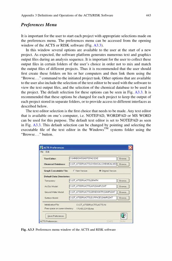
Open: Opens an existing ACTS/RISK data file. ACTS and RISK software use an

extension which is specific to models included in the software. When a user

database is saved, this specific extension is automatically added to the data file

stored. This data file can be found in the default data path chosen by the user under

the preferences menu. If the user has not modified this path, the data files will be

saved under the default ACTS and RISK folder paths. It is recommended that at the

start of a new project, specific folders be prepared and the default path be modified

to point to these folders using the preferences menu option. This process will allow

the user generated files to be sorted and saved in specific files related to the project.

This choice of specific folders to store the data in a specific session can be accessed

under the “Options!Preferences” pull down menu at the start of the ACTS/RISK

software as described above (Fig. A3.3).

Save: Saves the active data file with the name and location previously set in the

“Save As” dialogue box. When the user saves a data set for the first time ACTS

displays the “Save As” dialogue box. If the user prefers to change the name and

location of an existing data set, one should choose the “Save As” command from

the File menu.

Appendix 3 Definitions and Operations of the ACTS/RISK Software 445

Save As: Displays the “Save As” dialogue box. In this dialogue box one may

specify the name and location of the data file to be saved.

Print: Prints the active data file on the selected printer available on the computer.

Before one uses this command, one should install a printer. See the WINDOWSTM

documentation on how to install a printer on a computer. To select a printer and

adjust the parameter setting of a printer, choose “Printer Setup” from the file menu.

Printer Setup: Provides a list of installed printers, allows choosing the default

printer and setting other printing options.

Exit: Exits the model window. ACTS and RISK at this step prompts the user to

save any unsaved changes made to the data file. The data remains saved in the

memory unless one terminates the program by selecting “RETURN TO THE

MAIN SHELL” from the model window. The user may also choose the Edit

model option to return to the data saved from the main menu.

Calculate Menu

Executes the model equations based on the input data prepared. Any computational

error encountered during the execution will be displayed, and recommended

changes that are required to avoid the error will be displayed. Results are stored

in the memory to be displayed later on. At this stage, only a specific output

requested by the user at a certain spatial point and time is displayed in the analytical

calculation results grid in the input data window. The specification of this spatial

point and time is entered into the input data file by the user as will be described

below. If an input variable is using a Monte Carlo analysis generated set of values, a

“Monte Carlo” heading is displayed in the results grid. To view the complete

results, the user should choose the “View” or “Graph” menu option from the

“Results” menu. For the Air dispersion models the computation is only performed

using the “Current Chemical” data when multiple chemicals are selected. The

current chemical can be changed by a mouse click on the name of the chemical

in the analytical calculation results grid if more than one chemical is selected while

using the “Chemical” menu. Pressing function key F7 may also perform this

operation.

Results Menu

If the calculation performed is not a single output as displayed on the results grid, or

if at least one variable of the model is computed as a “Monte Carlo” variable, this

menu option allows viewing of the results in a bar chart or in other two- or three-

dimensional graphical formats.

Graph: Uses the built in graphics software to display the results. This option may

only be used if the “Monte Carlo” heading is displayed in the analytical result grid

for the current chemical, or the results are one-, two- and three-dimensional time

dependent or steady state results. Only these types of output can be displayed in

446 Appendix 3 Definitions and Operations of the ACTS/RISK Software

graphical format. If the model used generates only one output for the problem that is

not spatially variable or time independent, then the graph option cannot be used.

This is the case for some of the surface water pathway models. There are two

graphical packages that are available for the user. These are identified as: (i) New

Version; and, (ii) Original Version. The choice of using either of these graphic

packages needs to be made by the user at the start of the ACTS and RISK software.

This choice can be accessed under the “Options!Preferences” pull down menu at

the start of the ACTS/RISK software. The difference between these two graphical

packages is that the “New version” provides the user with more options to plot the

results of a computation. The use of the “Original Version” is initially recom-

mended since it will simplify the choices and the interface. Once a selection is

made, the “Save Preferences” button must be clicked to save the option that is

selected in the preferences window. Throughout the remaining session, and in

future sessions, the selected set of preferences will remain as the default selection

until a new selection is made during another session.

View: Displays numerical output generated for a simulation in a WINDOWSTM

Editor. The editor to be used for this purpose can be selected under the “Options!-

Preferences” menu at the start of the project as discussed earlier.

Special Menu (Only in AIR Pathway Model)

Use Same Soil and Physical Data: Allows the user to use the same input data for

all of the selected chemicals under the air dispersion models. Whenever the user

selects a different chemical, the data for soil and physical parameters of the

problem are copied from the old chemical input window to the newly selected

chemical input window. In this case the Monte Carlo simulation values are also

copied. The chemicals selected for an application remain unchanged when the

user saves the data file. The status of this option is also saved with the data file.

When the user opens the file during another time the same selection of chemicals

must be used, or one may restart a new project with a new set of chemical

selections if changes are necessary.

Note: Selection of this option will overwrite data from the old chemical to the

new selected chemical. The data for the newly selected chemical would be lost.

Chemical Constants Usage: Displays a dialogue box that indicates which proper-

ties of the selected chemicals are being used in the analytical computation.

Help Menu

Displays help for the current model. Function key F1 can also be used to display

related information. When selected, sections of help menu information will appear

as context sensitive information on the model used.

Appendix 3 Definitions and Operations of the ACTS/RISK Software 447

Chemical Menu Options

OK button: Choosing the OK button will allow the use of the chemicals listed in the

selected chemicals list box. Selecting Exit from the File menu is the same as

choosing OK.

Cancel button: Choosing this option will discard any changes made in the

chemical data editing process and will exit the chemical selection module with

the original selection intact.

Clear button: Unselects all of the selected chemicals. A loss of data in the

emission and concentration models may result if the OK or EXIT option are

selected after unselecting all chemicals. Choose CANCEL to undo the selection

process if the original files are to be kept.

Printing chemical properties: To print properties of the selected chemicals,

choose the Print option from the File menu. The software uses the default printer

defined in the print manager to print the text using the default editor. To select a

different printer choose Printer Setup from the file menu of the opening window of

the air model and make the appropriate selection at the beginning of the project.

Selection of chemicals: A chemical can be selected by moving the mouse

cursor to the left margin of the grid. When the left margin is reached the mouse

cursor becomes an arrow mark. Click the left mouse button on the row of the

chemical while pressing the “CTRL” button on the keyboard. The row color of

the selected chemical changes to red, which indicates the selection of the chemical.

All selected chemicals are also displayed in a list in the lower right corner of the

“Selected Chemicals” window. After the desired selections are made one may

choose the OK button to use the selected chemicals in the contaminant transport

and/or emission models of the air pathway. All chemical properties that are

necessary to execute the model in use will automatically be transferred from the

chemical database to the model data input grid. This process simplifies the chemical

properties data entry for the user. The user needs to be careful with the units of the

other parameters that are entered to execute a specific model. These units are

displayed on the data input window grid.

Unselecting the chemicals: To unselect a chemicalmove themouse cursor to the left

margin of the grid. The mouse cursor changes to an arrow mark. Click the left mouse

buttonwhile the “CTRL” button is depressed. The color of the row changes from red to

white and the chemical is unselected. If the user leaves thiswindowby selecting theOK

button at this stage, the unselected chemical will not be available for the next step of

calculations. To undo this change, one either has to re-select the chemical or choose the

“Cancel” option to disregard the changes made in the chemical selection operation. In

this case, the first selection made will be available for the next step.

Modifying Chemical Database: The ACTS software does not allow modification

of the CHEMICAL.MDB database, which is the master data file. There are two

other databases included in the software, CHEM1.MDB and CHEM2.MDB. These

two databases are duplicates of the CHEMICAL.MDB database and they are

editable. If either of these two databases is selected as the default database from

448 Appendix 3 Definitions and Operations of the ACTS/RISK Software

“Options ! Preferences” menu, then the “Chemicals” pull down menu in the

“Select Chemicals” window becomes active and editing of the database can pro-

ceed. All air model files save chemical properties data in addition to other input and

output data that are entered by the user. When the user opens a file, the chemical

properties are read and compared with the database. If the chemical properties in a

data file do not match the data in a default chemical database, a message box is

displayed indicating this discrepancy. This discrepancy occurs by changing the

chemical database after preparing an air pathway input data file or by changing the

chemical’s data in the input box grid, which is not usually recommended. In any

case, the user is given the choice to use either chemical properties from the default

chemical database selected or from those saved in the file. If the data saved in the

model option are selected the chemical database will be unaffected and the data

entered manually will be used. The user needs to be very careful in selecting this

option regarding the accuracy of the data used for a specific chemical.

Adding a new chemical: New chemicals can be added by selecting ADD NEW

from the CHEMICAL menu on the form. All chemicals must have different names

and symbols cannot be used as names. This operation is not available if the

Chemical database selected is the master dataset, which is not editable. When

adding a new chemical to a database, all of the chemical properties listed in the

table must be entered. Otherwise errors will result during the calculation steps since

multiple parameters are accessed by the models and this process is transparent to

the user. Leaving a parameter blank for a new chemical may initiate an error during

calculation if the model uses that parameter. When a new chemical is entered the

units of the data should match the units of the property as indicated in the title bar of

the chemical database. If this rule is not followed errors will occur.

Editing existing chemical: To change properties of the chemical, first select

ENABLE EDIT from the CHEMICAL menu. Then place the cursor on the box of

the chemical property to be changed and type in the new value. Moving to a

different row would result in updating the chemical property entered. The change

would be permanent and the old value would be lost. After editing is complete,

select the DISABLE EDIT option from the CHEMICAL menu to avoid any

accidental changes on the database during another session.

Deleting a chemical from the database: A chemical can be deleted by selecting

this option.

Note: For any given input file prepared and saved for the air pathway models, the

user can only use the same set of chemicals in all the emission and air dispersion

models. If this is not what is desired, that is if a new chemical needs to be introduced

a new data base must be prepared.

Monte Carlo Module of the ACTS/RISK Software

The transformation and transport of contaminants depends on media-specific para-

meters. Typically many of these parameters exhibit spatial and temporal variability

Appendix 3 Definitions and Operations of the ACTS/RISK Software 449

as well as variability due to measurement errors. ACTS/RISK software provides the

capability to analyze the impact of the uncertainty and variability in the model

inputs on the outputs, using the Monte Carlo simulation technique.

The Monte Carlo module allows the user to generate random variables for most

of the model parameters included in the ACTS/RISK software. Based on these

random variables, a one-stage or two-stage Monte Carlo simulation may be per-

formed in emission models, groundwater contaminant transport models, surface

water mixing models and air pathway models. Figure A3.4 shows a typical data

entry window for this operation. In this window, the upper workspace grid is the

input area and the lower grid is the output area.

In order to produce a Monte Carlo simulation, the user will first click an empty

box under the variant column of the input grid, which will lead to a list of all the

available variants of the model used, and will appear in a pull down window. From

this window, the user should select an appropriate variable for which a probability

density function will be generated. Once a selection is made, the value of the

parameter, as defined in the input database prepared by the user in the previous

data entry window, will automatically appear in the column identified as “Mean.”

Thus in the ACTS/RISK software, the input value for a parameter entered in the

input data window is always considered to be the mean value for that parameter

during the Monte Carlo analysis phase. However, the user has the option of

changing this value at this stage if desired. It is important to note that the intended

change will also alter the original value of the parameter in the parent model input

window. Next, the user should enter the minimum, the maximum, the variance and

the number of random parameters to be generated in the corresponding columns to

the right of the “Mean” column. The distribution type can be selected by placing the

Fig. A3.4 Monte Carlo input window

450 Appendix 3 Definitions and Operations of the ACTS/RISK Software

mouse cursor in the “Distribution Type” column and by double clicking the

selection that will appear in a pull down menu. The selection of one of the

distributions will place the desired distribution name into the “Distribution Type”

column. This completes the input data preparation phase of a Monte Carlo analysis.

After completing the input data entry for all desired variants that will be

generated randomly, the user may press the F7 button on the keyboard or click on

the “Generate” menu on the menu bar to calculate the distributions for all of the

selected variables. Output values will be displayed in the “Simulation Results” grid.

At this point several options are available to the user. To select a computed output

“Arithmetic Mean” or “Geometric Mean” or other representation of the data

generated as an input value to the parent model, the user should click on the

value box. The background color of this value box changes to red indicating the

selected value. This process allows the user, for example, to use the mean of

the randomly generated parameters as an input value in the parent model. When

the user exits the Monte Carlo window after this selection, the selected value will

appear in the input data box of the parameter in the model input data window. The

other option is to select all of the values generated for the specific parameter. To

initiate this option, the user should click on the variant name, first column on the

left, in the “Simulation Results” grid. Clicking there will change the background

color of the variant name selected to red. After completing either of these selec-

tions, the user will exit the Monte Carlo module by selecting the “EXIT” option

from the “FILE” menu. The selected parameter value(s) will automatically be

transferred to the parent model for use as simulation as Monte Carlo values. The

user may also unselect a selected value by clicking in the corresponding cell if

the choice was made in error, before exiting the Monte Carlo module. If no

selection is made and if the Monte Carlo module is exited, then the value returned

to the parent model will be the original value entered in the parent model. If this

value was modified in the “Mean” input box as described above, the returned value

will be the new value entered in the Monte Carlo input box. Whenever the model

file is saved, all of the associated Monte Carlo simulation results are saved in the

same file. In all ACTS/RISK simulations, Monte Carlo analysis may be performed

for multiple variants that appear in the first column of the input area for the model

selected in the previous step.

Display of Results in the GRAPHIX Module

Numerical results of parameter distributions computed in this window can be

displayed in graphical format on the screen, or hard copy printouts of these

distributions can be made if desired. For this choice “Options” menu will be used.

The options available in the graphics option include the choice of a display of the

results in “histogram”, “frequency distribution”, “cumulative frequency distribu-

tion”, “probability distribution”, “cumulative probability distribution” and “com-

plementary cumulative probability function” formats.

Appendix 3 Definitions and Operations of the ACTS/RISK Software 451

Description of Menu Options in the Monte CarloSimulation Window

File Menu: Same as Before

Print: Prints the active graph on the selected printer. Before using this command, a

printer must be installed. See the Windows documentation on how to install a

printer. To select a printer choose PRINTER SETUP from the file menu.

Exit: Ends the Monte Carlo simulation and returns to the parent model data entry

window. Any output values selected for a variant in the “Simulation Results” grid

are displayed in the parent model input box for the parameters. The data remains

saved in the memory unless the user terminates the program by selecting RETURN

TO THE MAIN SHELL from the initially selected pathway model window.

Generate: Generates a Monte Carlo probability density function for the pre-

selected parameters in the model. After selecting values from the output of the

Monte Carlo simulation window, as described above, the user may “Calculate” the

Monte Carlo simulation based analysis from the input window of the project by

closing the Monte Carlo window and returning to the input window. Any computa-

tional error encountered during this analytical calculation will also be displayed.

Output results of the Monte Carlo generation will be displayed in the lower grid.

For the air pathway, the computation is only performed on the “Current Chemi-

cal.” The current chemical can be changed by selecting CHEMICAL/MODEL from

the SELECT menu in the air pathway and unsaturated groundwater pathway

models. Simulation may also be performed by pressing the function key F7.

Graph: Displays the Monte Carlo simulation results in graphical format.

View: Displays the Monte Carlo simulation result on parameters in the text

editor.

Help: Displays help for the active model. Function key F1 can also be used to

display the help menu.

Graphics Module of the ACTS/RISK Software

The graphics module of the ACTS and RISK software uses the two different

graphics module software options identified as: (i) New Version; and, (ii) Original

Version, as outlined earlier. The selection for either of these options can be made in

the “Preferences” window as described above. The interface window for the two

graphics options is the same (Figs. A3.5–A3.7) with the only difference being that

the “New Version” selection provides an option to plot three-dimensional surface

plots of the output data as shown in Fig. A3.8. The use of the “Original Version” is

recommended initially since it will simplify the choices on the interface for a

novice user.

452 Appendix 3 Definitions and Operations of the ACTS/RISK Software

Fig. A3.5 Breakthrough

curve plot input window for

two-dimensional output data

Fig. A3.6 Normal curve plot

input window for two-

dimensional output data

Appendix 3 Definitions and Operations of the ACTS/RISK Software 453

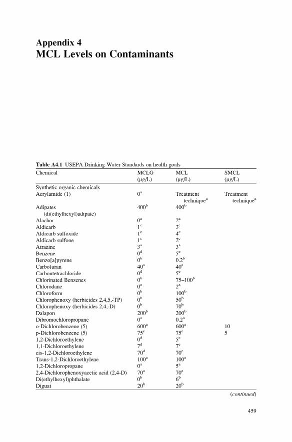
Fig. A3.8 Surface plot input

window for two-dimensional

output data

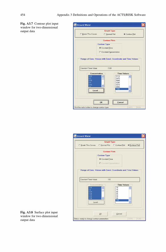
Fig. A3.7 Contour plot input

window for two-dimensional

output data

454 Appendix 3 Definitions and Operations of the ACTS/RISK Software

The first option to display the output is the plot of the breakthrough curves of

the output concentrations at one or more points of the solution domain. In Fig. A3.5

the selection options are shown for a two-dimensional model. In this case, first the

number of breakthrough curves that one would like to display will be entered (here

the default is 10) and then the (x, y) coordinates of the point where the output will

be displayed will be selected by clicking on the coordinate values in the x- and y-

coordinates window. All selections made will appear in the grid below the x- and

y-coordinates columns. If themodel used generates one-dimensional or three-dimen-

sional output the data entry window will automatically change, allowing only

for x-coordinate selection for one dimensional models or x-, y-, z-coordinate

selection for three dimensional models at this step. Once these selections are

made the user may click on the “OK” button to display the output in the desired

format. In the window where the graphical plot of the ACTS output is displayed

there are several other options which allow the user to modify the

output presented, such as the selection of the display colors, the type of lines

or symbols used, changing the title of the plot or the axis titles of the plot, and

finally adding footnotes to provide information about the plot prepared. All of

these options can be added to the plot generated using the pull downmenus at the top

bar of the plot window or by clicking in the various locations of the plot area where a

change or modification is desired. This process is the same in all figures that are

generated in the ACTS and RISK software. One should also notice that the user may

generate standard templates during this process, save templates generated or use an

existing template generated earlier in the current plot. All of these options can be

accessed from the pull down menu on the menu bar. It is recommended that the user

get familiar with this process by using the interface provided in the plot windowwhile

experimenting with test databases.

The second plot option is identified as the “Normal” plot, which implies that

the numerical results obtained from the ACTS software will be plotted as C(x),C(y) or C(z) results at various times. The input data entry window for this case is

shown in Fig. A3.6 where the input window for a two-dimensional model output

is displayed. As can be seen in Fig. A3.6, the option to select C(z) is inactive

since the output data is generated using a two-dimensional model. If the model

used is a one-dimensional model, the C(y) option will also be inactive. After

selecting which option to plot using the radio buttons, the user will again select

the number of plots to be displayed. This selection is followed by the selection of

the y-coordinates and time values of the desired C(x) plot. At this step, if one

selects to plot the C(y) plot, than the x-coordinates and time values of the desired

C(y) plot will be entered. As before, the selected coordinates will appear in the

grid below. Once the user is satisfied with the selections made, the “OK” button

can be clicked to display the graph. Similar to the case above the title, the axis

titles and footnotes can be added to the figure to finalize the plot. The templates

option is available in this case as well. It is recommended that the user get

familiar with this process by using the interface provided in the plot window

while experimenting with sample databases.

Appendix 3 Definitions and Operations of the ACTS/RISK Software 455

The third option that is available to the user is the possibility of displaying the

results of the computation in a contour plot format. This window is shown in

Fig. A3.7 for the case of a two-dimensional analysis. The contour plot option is not

available for one dimensional analysis since contour plots cannot be generated for

one-dimensional analysis. As such, this option is only available for two- or three-

dimensional analysis. As can be seen in Fig. A3.7 the choice for this case is the plot of

various concentration contours at a fixed time or the plot of the spatial variation of

constant concentrations at selected times. These selections can be made using the

radio buttons and the grid data that are available for the output generated during an

application. Once appropriate selections are made one may click on the “OK” button

to display the contour plot desired. As before the title, the axis titles and footnotes can

be added to the figure to finalize the plot in the plot window. The templates option is

also available in this case aswell. It is recommended that the user get familiar with this

process by using the interface provided in the plot window while using sample data

files provided.

The fourth option that is available to the user is the possibility of displaying the

results of the computation in a surface plot format. This option is only available if

the “New Version” of the graphics module is selected as the default graphics

module in the preferences window as discussed above. This window is shown in

Fig. A3.8 for the case of a two-dimensional analysis. The surface contour plot

option is not available for one dimensional analysis since surface contour plots

cannot be generated for one-dimensional analysis. As such, this option is only

available for two- or three-dimensional analysis results. As can be seen in

Fig. A3.8 the choice for this case is the plot of various concentration contours

at a fixed time, or the plot of the constant concentration at selected times as

described above for the contour plot option. These selections can be made using

the radio buttons and the grid data that are available for the output generated

during an application. Once appropriate selections are made, one may click on the

“OK” button to display the surface plot desired. As before the title, the axis titles

and footnotes can be added to the figure to finalize the plot in the plot window.

The templates option is available in this case as well. It is recommended that the

user get familiar with this process by using the interface provided in the plot

window and the sample data files provided.

The operational characteristics of these plotting routines are standardized such

that all modules in the ACTS and RISK software use the same interface. One

should also notice that the graphics package that displays the statistical analysis

is the same as the one discussed in this appendix. However, in the case of a RISK

model, only the bar charts, the statistical output or the probability density

functions of the statistical output can be displayed. The user, through practice,

may immediately recognize that the procedures that are used to change the titles,

colors and displayed lines follow the same procedures described in this appendix.

Familiarity with these procedures may only be achieved through practicing the

different options that are available in each window.

456 Appendix 3 Definitions and Operations of the ACTS/RISK Software

Rules for Data Entry in a Typical Input Window

The data entry procedure for all models follows a very simple rule. The discretiza-

tion of the selected coordinate axis will follow the following format described

below as shown in Fig. A3.9. To discretize the x-coordinate, the beginning value

(minimum), the final value (maximum), the discretization interval (step size) and

the constant value are entered while separating the data entry values with (:) as

shown below and in Fig. A3.9.

0:3200:50:800

The last data entry need not be entered, in which case the maximum value will be

selected as the constant value from which the concentration will be computed and

displayed in the output grid below. As the data are entered, the user will recognize

the reflection of the input in the output grid below. The other coordinate discretiza-

tion data follows the same format.

This is the only data entry procedure that is standardized according to a format.

The other data entry options in the “Boundary Conditions” and “Field and Chemical

Constants” folders will follow a simple numerical data entry action.

Fig. A3.9 Standard data entry window for groundwater module

Appendix 3 Definitions and Operations of the ACTS/RISK Software 457

Appendix 4

MCL Levels on Contaminants

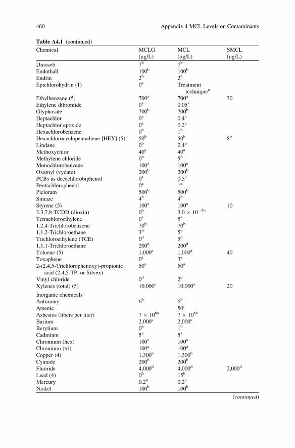
Table A4.1 USEPA Drinking-Water Standards on health goals

Chemical MCLG

(mg/L)MCL

(mg/L)SMCL

(mg/L)Synthetic organic chemicals

Acrylamide (1) 0a Treatment

techniqueaTreatment

techniquea

Adipates

(di(ethylhexyl)adipate)

400b 400b

Alachor 0a 2a

Aldicarb 1c 3c

Aldicarb sulfoxide 1c 4c

Aldicarb sulfone 1c 2c

Atrazine 3a 3a

Benzene 0d 5e

Benzo[a]pyrene 0b 0.2b

Carbofuran 40a 40a

Carbontetrachloride 0d 5e

Chlorinated Benzenes 0b 75–100b

Chlorodane 0a 2a

Chloroform 0b 100b

Chlorophenoxy (herbicides 2,4,5,-TP) 0b 50b

Chlorophenoxy (herbicides 2,4,-D) 0b 70b

Dalapon 200b 200b

Dibromochloropropane 0a 0.2a

o-Dichlorobenzene (5) 600a 600a 10

p-Dichlorobenzene (5) 75e 75e 5

1,2-Dichloroethylene 0d 5e

1,1-Dichloroethylene 7d 7e

cis-1,2-Dichloroethylene 70d 70e

Trans-1,2-Dichloroethylene 100a 100a

1,2-Dichloropropane 0a 5a

2,4-Dichlorophenoxyacetic acid (2,4-D) 70a 70a

Di(ethylhexyl)phthalate 0b 6b

Diguat 20b 20b

(continued)

459

Table A4.1 (continued)

Chemical MCLG

(mg/L)MCL

(mg/L)SMCL

(mg/L)Dinoseb 7b 7b

Endothall 100b 100b

Endrin 2b 2b

Epichlorohydrin (1) 0a Treatment

techniquea

Ethylbenzene (5) 700a 700a 30

Ethylene dibromide 0a 0.05a

Glyphosate 700b 700b

Heptachlor 0a 0.4a

Heptachlor epoxide 0a 0.2a

Hexachlorobenzene 0b 1b

Hexachlorocyclopentadiene [HEX] (5) 50b 50b 8b

Lindane 0b 0.4b

Methoxychlor 40a 40a

Methylene chloride 0b 5b

Monochlorobenzene 100a 100a

Oxamyl (vydate) 200b 200b

PCBs as decachlorobiphenol 0a 0.5a

Pentachlorophenol 0a 1a

Picloram 500b 500b

Simaze 4b 4b

Styrene (5) 100a 100a 10

2,3,7,8-TCDD (dioxin) 0b 3.0 � 10�5b

Tetrachloroethylene 0a 5a

1,2,4-Trichlorobenzene 70b 70b

1,1,2-Trichloroethane 3b 5b

Trichloroethylene (TCE) 0d 5d

1,1,1-Trichloroethane 200d 200d

Toluene (5) 1,000a 1,000a 40

Toxaphene 0a 3a

2-(2,4,5-Trichlorophenoxy)-propionic

acid (2,4,5-TP, or Silvex)

50a 50a

Vinyl chloride 0d 2d

Xylenes (total) (5) 10,000a 10,000a 20

Inorganic chemicals

Antimony 6b 6b

Arsenic 50i

Asbestos (fibers per liter) 7 � 106a 7 � 106a

Barium 2,000c 2,000c

Berylium 0b 1b

Cadmium 5a 5a

Chromium (hex) 100a 100a

Chromium (tri) 100a 100a

Copper (4) 1,300h 1,300h

Cyanide 200b 200b

Fluoride 4,000d 4,000d 2,000d

Lead (4) 0h 15h

Mercury 0.2h 0.2a

Nickel 100b 100b

(continued)

460 Appendix 4 MCL Levels on Contaminants

Table A4.1 (continued)

Chemical MCLG

(mg/L)MCL

(mg/L)SMCL

(mg/L)Nitrate (as N) (2) 10,000a 10,000a

Nitrite (as N) 1,000a 1,000a

Selenium 50a 50a

Silver 100

Sulfate 5 � 105b 5 � 105b

Thallium 0.5b 2b

Microbiological parameters

Bacteria <1/100 ml

Giardic lamblia 0 Organismsf

Legionella 0 Organismsf

Heterotropic bacteria 0 Organismsf

Viruses 0 Organismsf

Radionuclides

Radium 226 (3) 0g 20 pCi/Lg

Radium 228 (3) 0g 20 pCi/Lg

Radon 222 0g 300 pCi/Lg

Uranium 0g 20 mg/L(30 pCi/L)g

Beta and Photon emitters (excluding

radium 228)

0g 4 mrem ede/yearg

Adjusted gross alpha emitters (excluding

radium 226, uranium and radon 222)

0g 15 pCi/Lg

A pCi (picocorrie) is a measure of the rate of radioactive disintegration. Mrem ede/year is a

measure of the dose of radiation received by either the whole body or a single organ

1. This is a chemical used in treatment of drinking water supplies. The U.S. EPA specifies how

much may be used in the treatment process. It would be unlikely to find this chemical in

contaminated water

2. The total nitrate plus nitrite cannot exceed 10 mg/L

3. This MCL would replace the current MCL of 5 pCi/L for combined 226 Rsa and 228 Ra. The

radionuclide rules were under review as of Spring, 1997

4. There is no MCL for copper and lead. The U.S. EPA requires the treatment of water before it

enters a distribution system to reduce the corrosiveness so that these chemicals do not leach from

the distribution system back into the water supply

5. SMCL is a suggested value only. Concentrations above this level may cause adverse taste in

water. See Federal Register, January 30, 1991

6. The MCL for arsenic is under review as of Spring, 1997aFinal value. Published in Federal Register, January 30, 1991bFinal value. Published in Federal Register, July 17, 1992cFinal value. Published in Federal Register, July 1, 1991dFinal value. Published in Federal Register, April 2, 1986eFinal value. Published in Federal Register, July 7, 1987fFinal value. Published in Federal Register, June 29, 1989gProposed value. Published in Federal Register, July 18, 1991hFinal value. Published in Federal Register, July 7, 1991iProposed l value. Published in Federal Register, November 13, 1985jProposed value. Published in Federal Register, February 12, 1978

Appendix 4 MCL Levels on Contaminants 461

Appendix 5

Conversion Tables and Properties of Water

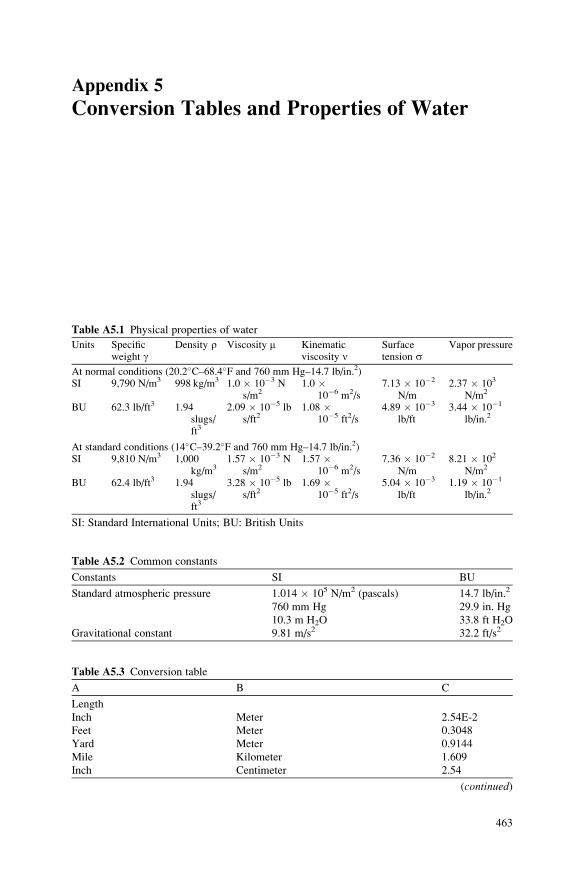
Table A5.1 Physical properties of water

Units Specificweight g

Density r Viscosity m Kinematicviscosity n

Surfacetension s

Vapor pressure

At normal conditions (20.2�C–68.4�F and 760 mm Hg–14.7 lb/in.2)SI 9,790 N/m3 998 kg/m3 1.0 � 10�3 N

s/m21.0 �

10�6 m2/s7.13 � 10�2

N/m2.37 � 103

N/m2

BU 62.3 lb/ft3 1.94slugs/ft3

2.09 � 10�5 lbs/ft2

1.08 �10�5 ft2/s

4.89 � 10�3

lb/ft3.44 � 10�1

lb/in.2

At standard conditions (14�C–39.2�F and 760 mm Hg–14.7 lb/in.2)SI 9,810 N/m3 1,000

kg/m31.57 � 10�3 N

s/m21.57 �

10�6 m2/s7.36 � 10�2

N/m8.21 � 102

N/m2

BU 62.4 lb/ft3 1.94slugs/ft3

3.28 � 10�5 lbs/ft2

1.69 �10�5 ft2/s

5.04 � 10�3

lb/ft1.19 � 10�1

lb/in.2

SI: Standard International Units; BU: British Units

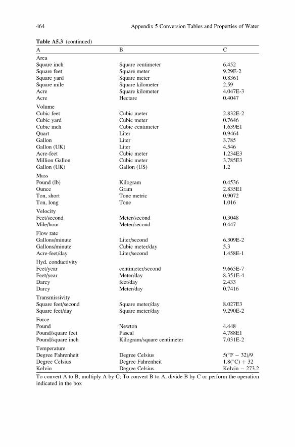
Table A5.3 Conversion table

A B C

Length

Inch Meter 2.54E-2

Feet Meter 0.3048

Yard Meter 0.9144

Mile Kilometer 1.609

Inch Centimeter 2.54

(continued)

Table A5.2 Common constants

Constants SI BU

Standard atmospheric pressure 1.014 � 105 N/m2 (pascals) 14.7 lb/in.2

760 mm Hg 29.9 in. Hg

10.3 m H2O 33.8 ft H2O

Gravitational constant 9.81 m/s2 32.2 ft/s2

463

Table A5.3 (continued)

A B C

Area

Square inch Square centimeter 6.452

Square feet Square meter 9.29E-2

Square yard Square meter 0.8361

Square mile Square kilometer 2.59

Acre Square kilometer 4.047E-3

Acre Hectare 0.4047

Volume

Cubic feet Cubic meter 2.832E-2

Cubic yard Cubic meter 0.7646

Cubic inch Cubic centimeter 1.639E1

Quart Liter 0.9464

Gallon Liter 3.785

Gallon (UK) Liter 4.546

Acre-feet Cubic meter 1.234E3

Million Gallon Cubic meter 3.785E3

Gallon (UK) Gallon (US) 1.2

Mass

Pound (lb) Kilogram 0.4536

Ounce Gram 2.835E1

Ton, short Tone metric 0.9072

Ton, long Tone 1.016

Velocity

Feet/second Meter/second 0.3048

Mile/hour Meter/second 0.447

Flow rate

Gallons/minute Liter/second 6.309E-2

Gallons/minute Cubic meter/day 5.3

Acre-feet/day Liter/second 1.458E-1

Hyd. conductivity

Feet/year centimeter/second 9.665E-7

Feet/year Meter/day 8.351E-4

Darcy feet/day 2.433

Darcy Meter/day 0.7416

Transmissivity

Square feet/second Square meter/day 8.027E3

Square feet/day Square meter/day 9.290E-2

Force

Pound Newton 4.448

Pound/square feet Pascal 4.788E1

Pound/square inch Kilogram/square centimeter 7.031E-2

Temperature

Degree Fahrenheit Degree Celsius 5(�F � 32)/9

Degree Celsius Degree Fahrenheit 1.8(�C) þ 32

Kelvin Degree Celsius Kelvin � 273.2

To convert A to B, multiply A by C; To convert B to A, divide B by C or perform the operation

indicated in the box

464 Appendix 5 Conversion Tables and Properties of Water

Index

A

Adsobtion, 86, 87, 90

Advection, 12, 15, 20, 67, 69, 77, 78, 83, 86,

91–93, 112, 124, 135, 136, 151, 187,

192–195, 197, 206, 207, 210, 225, 231,

232, 236, 242, 243, 253, 255, 257, 283,

308, 311–315, 358, 417

advective flux, 70, 74

Air dispersion model

box dispersion model, 136–138

Gaussian dispersion model, 138–148

indoor air dispersion, 110, 149–152

Air emission

air emission rate, 113, 166, 172

indoor emission, 130, 149–152, 159–161

landfill emission, 127–129

vapor emission, 114

Air pathway

Cowherd particulate emission model, 108,

120–124

Farmer’s model, 113–117, 119, 126, 169

Jury model, 124–126

landfill gas emission model, 108

steady state models, 138, 147

Thibodeaux–Wang model, 108, 117–120

unsteady state models, 110

volatilization, 108, 119, 124, 125, 130–134,

149, 181, 182, 184

volatilization from water, 108, 130–134,

181, 182

Anthropogenic, 127

Aquiclude, 188

Aquifer

confined aquifer, 188, 204

finite aquifer, 206–208, 212, 218, 221–223

infinite aquifer, 203, 210, 214–225,

232, 386

semi confined aquifer, 188

semi infinite aquifer, 203, 205,

208–211, 218

unconfined aquifer, 188, 204, 254, 257,

379, 381

Aquifuge, 188

Aquitard, 188

B

Boundary condition

Cauchy boundary condition, 200, 202, 204,

205, 207–210

Dirichlet boundary condition, 91, 196–198,

202, 204–209

Neuman boundary condition, 92, 205

Buoyancy

buoyancy effect, 142, 292, 294

buoyancy flux, 143–146, 295

buoyancy plume, 143, 293, 302, 305

C

Calibration

calibration parameter, 47

model calibration, 45–50, 392, 405

Cancer slope factor (CSF), 362, 363

Capillary

capillary height, 190

capillary zone, 154–155, 189

Characterization, 5, 9, 16, 23, 25, 26, 40, 98,

162, 192, 277, 292, 296, 360, 414, 436

site characterization, 162

Chezy equation, 281

Chezy coefficient, 282

465

Conduction, 15, 67, 70, 72, 79

Conservation

conservation of energy, 72, 78, 79

conservation of mass, 9, 16, 19, 70, 73, 74,

76, 77, 80–83, 193, 286, 289, 290

conservation of momentum, 73

conservation principles, 63–93

Continuity, 44, 77, 81, 288

continuity principle, 44, 81

Control volume, 12, 13, 15, 66, 73–75, 84, 101,

189, 418, 421, 422

representative elementary control volume,

13, 66, 280

Convection, 15, 67, 160

Cross currents

stagnant cross current, 298–300, 302–303

weak cross current, 298–300, 302–303

D

Darcy law

Darcy velocity, 191

pore velocity, 191

Decay

decay coefficient, 136, 204, 207–210, 232,

309, 315, 318

decay rate, 124, 126, 141, 178, 207, 233,

256, 287, 291, 312, 323

Density, 21, 31, 67, 71–73, 83, 100–103, 115,

118, 130, 143, 145, 152, 153, 155, 163,

168–171, 181, 183, 184, 191, 195, 204,

255, 258, 259, 264, 265, 284, 292–298,

300, 313, 324, 326–329, 336, 339–348,

373–376, 386, 387, 392, 397

Deposition, 14, 15, 146, 148, 277, 319, 322

Diffusion

diffusion coefficient, 14, 29, 70, 71, 92,

114, 115, 124, 126, 132, 135, 136, 151,

154–156, 206, 212, 219, 230, 232, 257,

258, 309, 335, 337

diffusion process, 69, 112, 114, 193, 276

diffusive flux, 68, 69

mechanical mixing, 193

molecular diffusion, 120, 193

turbulent diffusion, 309

Dilution, 210, 213, 276, 283, 291, 292, 294,

298–308, 328–330

Dispersion

constant dispersion model, 200, 202, 225

hydrodynamic dispersion, 193, 194, 204,

206, 207, 231, 233, 236, 237, 255, 267

lateral dispersion, 107

longitudinal dispersion, 194, 208, 259,

264–266, 311, 312, 320

transverse dispersion, 194, 210, 222, 233,

264, 311, 387

variable dispersion model, 232

Distribution

exponential distribution, 346

Gaussian distribution, 141, 195, 196, 216,

242, 392

lognormal distribution, 172, 173, 344,

345, 347

normal distribution, 135, 147, 170–172,

326, 327, 342–344, 373

triangular distribution, 347

uniform distribution, 347, 348

Dose

chronic reference dose, 362

dose response, 25–27

exposure dose, 7, 25, 26, 358, 360, 361, 365

reference dose, 362, 364

sub-chronic reference dose, 362

E

Energy

conservation of energy, 72, 78, 79

energy flux, 72, 73

Environmental health, 1, 5, 9, 10, 18, 19, 21,

22, 25, 26, 28, 29, 33, 34, 59, 381,

386, 441

environmental management, 1–4, 9, 10,

17, 64

Epidemiology, 5, 28, 437–438

environmental epidemiology, 28

Estuary, 32, 293, 295, 313, 317, 320–322

estuary model, 295

Expected value, 49, 339–341, 343, 346,

349, 353

Exposure

exposure analysis, 5, 6, 23–25, 29, 32,

33, 137, 163, 172, 277, 312, 349, 359,

360, 370

exposure dose, 7, 25, 26, 358, 360, 361, 365

exposure risk, 64, 149, 163, 357, 369

F

Far field, 292, 296, 307–316, 442

far field model, 306–316

Field capacity, 191

G

Gaussian source, 196, 201, 210, 214, 216

Gaussian source boundary, 214

Gradually varied flow, 279

Groundwater pathway

by-product model, 225–230

466 Index

by-products, 198, 200, 225

constant dispersion, 199, 200, 202–225,

236, 238, 242, 245

continuous source, 223, 224

instantaneous source, 217, 232, 246–253

Marino model, 254–257

multispecies, 198, 225

one dimensional model, 206, 210

point source, 210, 216–221, 238–240,

246–253, 265, 267

patch source, 212, 221, 222

saturated zone, 188, 191, 204, 206, 212,

219, 230, 232, 254

three dimensional models, 200, 202, 218

two dimensional models, 210–218

unsaturated zone, 254–259

variable dispersion, 231–254, 269

H

Half life, 85, 207, 260, 266, 277, 309, 314,

315, 330, 387

Hazard

hazard control, 434

hazard identification, 24, 25

Henry’s law, 114, 130, 131, 133, 152, 153

Hydraulic conductivity, 191, 192, 194, 393

Hydrodynamic mixing, 313

I

Infiltration, 126, 210, 213, 259

Insolation, 105, 106, 142, 178

Intake

intake model, 364–369

intake rate, 25, 26, 359, 361, 363, 366

Isotherm

Freundlich isotherm, 88, 89

Langmuir isotherm, 87, 89, 90

linear isotherm, 87, 132

L

Lakes

great lakes, 130, 276, 295, 314–316

oceans, 275, 295, 314–316

reservoirs, 275, 276, 308, 314

small lakes, 290–291, 295, 308, 314

Lapse rate

adiabatic lapse rate (ALR), 98, 100,

103, 144

dry adiabatic lapse rate, 98

environmental lapse rate (ELR), 98,

100, 104

saturated adiabatic lapse rate (SALR),

98–100

M

Manning’s equation, 43

Manning’s coefficient, 282, 283

Mass

conservation of mass, 9, 16, 19, 70, 73, 74,

76, 77, 80–83, 193, 286, 289, 290, 421

mass balance, 12, 15, 33, 68, 69, 135, 136,

286–288, 290, 291, 319, 323, 403, 422

mass flux, 15, 16, 70, 71, 74, 75

Mean, 31, 58, 69, 137, 143, 155, 159, 169, 175,

205, 267, 283, 286, 287, 289, 297, 312,

313, 326, 339–345, 347–349, 351, 352,

389–391, 393, 394, 450, 451

mean value, 49, 57, 168, 325, 336, 389, 393,

394, 401, 450

Median, 169, 327, 343, 345, 365

Mixing model

buoyant jet, 295, 298, 300–302

deep receiving water, 298, 301, 302,

305–306, 325

eddy mixing, 284, 285

far field mixing, 291, 292, 294, 295,

307–316

intermediate zone, 189

longitudinal mixing, 285, 287

near field mixing, 292, 294–307

pure jet, 295, 298

pure plume, 295, 298

shallow receiving water, 298–299, 301,

303, 306–307

transverse mixing, 284, 293, 308–310

Mode, 21, 29, 31, 59, 110, 138, 181, 187, 262,

277, 333, 343, 345, 371–373

Modeling

continuous, 44

deterministic, 16, 19, 44, 187, 277,

395–396, 401, 403

discrete, 44

dynamic, 44, 66, 441

environmental modeling, 4, 9, 15, 17–21,

23–25, 37–59, 64, 66, 67, 344, 358, 409,

417–438

linear, 44

model building, 17, 20, 33, 37, 38,

41–46, 55

model calibration, 45–50, 392, 395, 405

modeling principles, 29, 40–41

modeling terminology, 39, 47, 59

model scale, 50–58

model types, 41–45, 111, 199

model uncertainty, 48

model validation, 47–48

model verification, 47

Index 467

Modeling (cont.)nonlinear, 44–45, 52, 53

probabilistic, 396–401

static, 44

stochastic, 21, 44, 47, 59, 66, 187, 231, 277,

335, 348, 424

Moisture, 54, 122, 124, 128, 157, 188–191

moisture content, 121, 190

Momentum

conservation of momentum, 19, 421

momentum balance, 67

momentum flux, 71–72, 145, 146, 295

Monte Carlo

Monte Carlo analysis, 21, 29, 42, 58, 116,

119, 123, 126, 129, 133, 134, 137, 138,

148, 166, 168–171, 175, 178, 181, 182,

205, 264, 266, 295, 325, 327, 328,

335–339, 341, 348–352, 371, 373,

374, 442, 446, 450, 451

Monte Carlo method, 29, 33, 129, 134, 148,

326, 333, 336, 350, 422

N

Near field, 33, 276, 291–294, 308, 315, 325,

329, 380, 441

near field model, 295–307, 310

Nonuniform flow, 278, 279

O

Oatland island

ecological management, 381

Oatland island study, 381, 382, 388–391

type curves, 398–403, 405

wetlands, 381, 394, 404

P

Partition coefficient, 88, 115, 153, 157, 206,

212, 219, 230, 257, 258, 320, 391

Peclet number, 78, 283

Pollutant, 5, 11, 12, 20, 97, 105, 106, 112, 127,

141, 142, 144, 276, 277, 283, 294, 313,

314, 418, 429, 431, 432

criteria pollutant, 96, 98

Porosity, 13, 14, 75, 76, 83, 115, 126, 153, 154,

156, 159, 163, 168–172, 189–191, 204,

206, 210, 236, 243, 255, 258, 259, 265,

267, 388, 391, 393

effective porosity, 189, 191

Probability

complementary cumulative probability,

328, 375, 376

cumulative probability, 328, 338–340, 343,

348, 350, 375, 376, 398, 451

probability density, 21, 31, 168–171, 181,

183, 184, 211, 264–266, 326–328, 336,

338, 340–348, 373–376, 392, 397, 423,

452, 456

probability distribution, 21, 116, 119, 123,

126, 129, 137, 148, 159, 205, 334,

336–341, 349, 350, 451

probability theory, 337–341

random variable, 205, 264, 334, 337–342,

344, 348, 349, 351

Processes

chemical processes, 11, 365

environmental processes, 11–17, 39, 42,

50–52, 333

geologic processes, 4, 188, 192, 417,

418, 420

R

Random

random error, 56

random number, 170, 171, 173, 326, 373

random variable, 205, 264, 334, 337–342,

344, 348, 349, 351, 424, 450

Rapidly varied flow, 279

Reaction

chemical reaction, 42, 52, 83, 84, 96,

192, 418

first order reaction, 42, 84–86, 210,

260, 266

heterogeneous reaction, 86–91, 206, 207,

212, 220, 230, 232

homogeneous reaction, 83–86

irreversible reaction, 91

reversible reaction, 91

Retardation, 225, 227, 255, 419

retardation coefficient, 29, 86, 88, 204,

206–210, 212, 213, 218, 220, 230,

232–234, 262, 267, 389, 391,

393, 419

Risk

cancer risk, 27, 363–364, 437

dermal, 5, 23, 24, 29, 31–33, 359–362,

364–368, 442

environmental risk, 24–28, 379–405,

433–437

health risk, 6, 9, 16–19, 23–27, 29, 32, 33,

40, 65, 172, 175, 334, 353, 357–376,

409, 417, 439, 441

ingestion risk, 5, 23, 25, 29, 31–33,

360–369, 371, 442

inhalation risk, 6, 23–25, 29, 31–33, 149,

163, 175, 358, 360–366, 368, 435, 442

minimal risk, 362–363

468 Index

risk analysis, 1, 9, 16, 17, 23–28, 33, 40,

357–376, 409, 417, 433–437, 439, 441

risk assessment, 5–7, 9, 18, 19, 22–27, 29,

32, 33, 64, 119, 357–364, 412, 430, 432,

435–437

risk characterization, 25, 26, 436

risk communication, 26, 436–437

risk management (RM), 25, 26, 65, 413,

436, 437

risk reduction, 437

S

Saturated zone, 32, 188, 191, 204, 206, 212,

219, 230, 232, 254, 379, 403, 404, 441

Saturation, 99, 100, 157, 160, 189, 190, 255

saturation constant, 86

Scale

functional scale, 53–55

macro scale, 14, 39

mega scale, 14, 68

micro scale, 14, 37, 39, 68

model scale, 50–58

molecular scale, 14, 37

Sediments

coastal water sediments, 295, 317, 322

estuary sediments, 295, 317, 320–321

lake sediments, 322–324

ocean sediments, 317, 322

river bed sediments, 317–320

surface water sediments, 316–324

Sensitivity, 42, 49, 58, 59, 302, 433

sensitivity analysis, 17, 45–50, 56, 59, 66,

205, 211, 335, 371, 380, 423–424

Shear stress

shear velocity, 283, 284, 309

wall shear, 281, 283, 284

Simulation, 16–19, 25, 29, 31, 32, 40–42, 45,

47, 48, 51, 53, 54, 56, 110, 150, 159,

200, 260, 334, 341, 348–352, 379, 381,

386–405, 421, 424, 439, 441, 447,

450–452

Sink, 9, 15, 74, 76, 78–82, 105, 139, 193, 195,

292, 293

Slope factor, 26, 27, 414, 437

Soil moisture, 121, 122, 157, 190

Sorption, 83, 86, 160, 417, 420, 441

Source, 6–10, 15, 19, 23, 24, 31–33, 54, 64, 65,

74, 76, 78–82, 91, 95, 106, 108–110,

112–114, 116, 120, 124, 125, 127, 133,

134, 136, 138, 141–143, 146–148,

150–153, 156, 158–162, 175–181, 193,

195–197, 200, 203–205, 210–225, 231,

232, 238–240, 242, 244–256, 260, 262,

263, 265, 267, 275, 277, 291, 307, 308,

310–313, 315, 317, 335, 349, 350, 358,

365, 366, 379–383, 386–400, 402–405,

422, 423, 428, 431, 434, 437

Specific yield, 191

Stability

absolute instability, 100

absolute stability, 100

atmospheric instability, 99

atmospheric stability, 98–107, 141, 142

conditional instability, 100

natural instability, 100

Pasquill stability, 105, 106, 142

potential instability, 100

Standard deviation, 58, 141, 196, 309, 311,

336, 339, 341, 343, 344, 347, 349,

391, 393

Stochastic, 44, 47, 59, 66, 187, 231, 277, 334,

348, 424

stochastic model, 21, 44, 47, 59, 66, 187,

335, 348, 424

Submerged discharge, 300–303

multiport diffusers, 304–307, 329

Superposition, 44, 125, 126, 198, 213, 218,

220, 222, 225, 232, 235, 262

method of superposition, 196, 197, 213, 218

Surface discharge, 297–300, 303, 310

surface point discharge, 297–301

Surface water pathway, 6, 18, 29, 33, 64, 65,

75, 86, 275–330, 336, 420, 441, 447

Sustainability, 4

T

Tidal effects, 293, 387

Toxicology

applied toxicology, 22

descriptive toxicology, 22

mechanistic toxicology, 22

U

Uncertainty

data uncertainty, 56

model uncertainty, 39, 48

prediction uncertainty, 48, 56, 138, 349,

421, 423, 424

uncertainty analysis, 17, 29, 32, 56, 110,

116, 119, 123, 126, 129, 134, 137, 148,

159–162, 205, 267, 330, 335, 336,

352–354, 367, 423, 424

Uniform flow, 279–284, 315

Unsaturated zone, 32, 52, 54, 55, 108,

124–126, 155–156, 162, 188–200,

254–257, 404

Index 469

V

Validation, 33, 45–50, 424

model validation, 47–48

Variability

parameter variability, 14, 334

variability analysis, 333–354

Variance, 16, 17, 49, 57, 58, 159, 170, 205,

334, 336, 340–346, 348, 351, 352,

373, 394, 450

Ventilation, 151, 156

Verification, 33, 45–50, 59, 424

model verification, 47

Volatilization, 108, 119, 124, 125, 130–134,

149, 181, 182, 184, 257, 420

W

Water saturation, 99, 189, 190, 255

470 Index