Geographical distribution of fresh citrus fruit production
110
APPENDIX 2
FUEL ECONOMICS FOR DIESEL FUEL
AND ORANGE OIL
The use of alternate fuels in internal combustion engines depends
on the technical feasibility and economic viability. Although many alternative
fuels are technically feasible they are not used in internal combustion engines
due to their higher cost. From the consumer’s point of view fuel cost is a
predominant factor. The fuel cost is calculated based on the availability,
production methods, transportation and energy equivalent to petroleum
products. The fuel economics of orange is calculated and compared with
diesel fuel as given below:
Fuel Economics of Diesel Fuel
Cost of the Diesel fuel for 1 liter (i.e. 0.830 kg) = Rs 39 Cost of 1 kg of diesel fuel = Rs 47 Cost of Diesel fuel consumed per hour = 1.28 kg × 47 = Rs 60.16 Brake Specific Fuel Consumption = 1.28/ 4.4 = 0.290 kg/kW h Cost for one unit of power produced per hour = 0.29 × 47= 13.63 Rs / kW h
(OR) Brake Specific Energy Consumption = BSFC × CV = 0.290 × 43000
= 12,470 kJ/kW h
111
Cost required to produce 1 kJ of energy from diesel fuel = 12470 × 0.001093
= 13.629 Rs /kW h
Fuel Economics of Orange Oil
Cost of orange oil for 1 liter (ie 0.816 kg) = Rs 125 Cost for 1 kg of orange oil = Rs 153 Cost of orange oil consumed per hour = 1.48 kg × 153 = Rs 226.44 Brake Specific Fuel Consumption = 1.48/ 4.4 = 0.336 kg/kW h Cost for one unit of power produced per hour = 0.336 × 153 = 51.4 Rs / kW h
(OR) Brake Specific Energy Consumption = BSFC × CV = 0.336 × 34650 = 11642.4 kJ / kW h Cost required to produce 1 kJ of energy from orange oil = 11642.4 × 0.004421
= 51.47 Rs/kW h Cost is higher for orange oil = 51.4 / 13.63 = 3.77
The cost of orange oil is higher by 3.77 times than that of diesel
fuel for producing one unit of power output per one hour. However the cost of
orange oil can be reduced when orange oil is produced on a large scale.
112
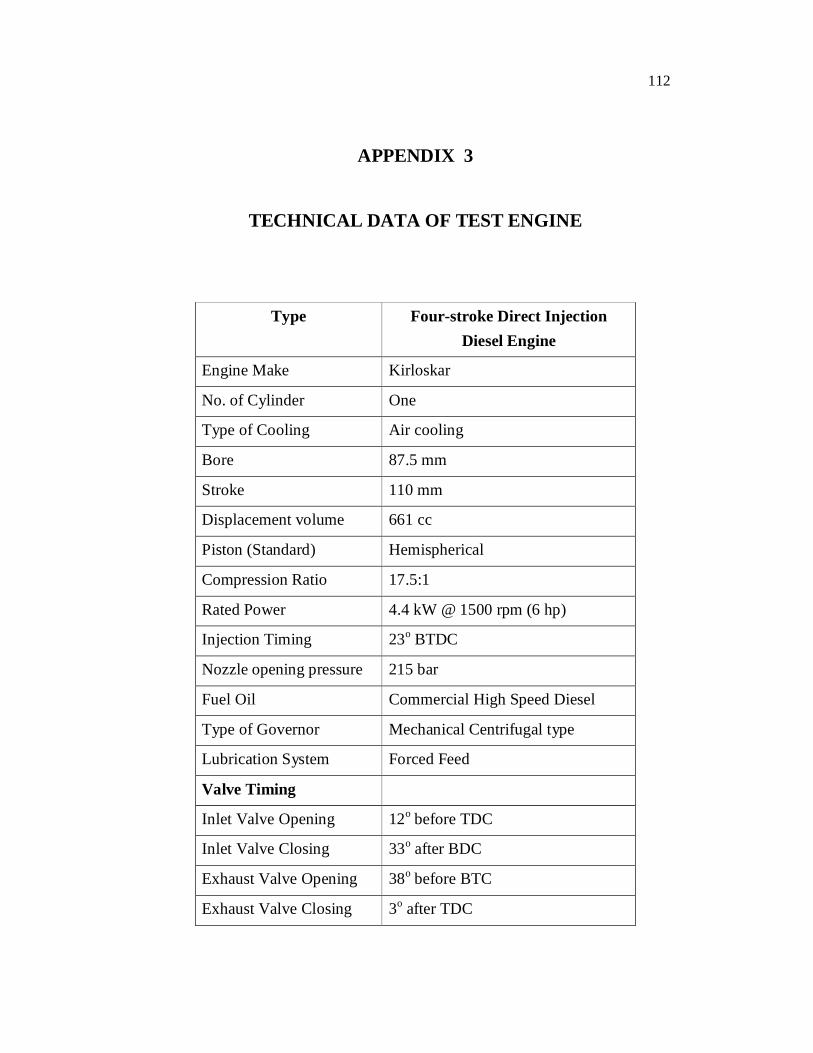
APPENDIX 3
TECHNICAL DATA OF TEST ENGINE
Type Four-stroke Direct Injection Diesel Engine
Engine Make Kirloskar
No. of Cylinder One
Type of Cooling Air cooling
Bore 87.5 mm
Stroke 110 mm
Displacement volume 661 cc
Piston (Standard) Hemispherical
Compression Ratio 17.5:1
Rated Power 4.4 kW @ 1500 rpm (6 hp)
Injection Timing 23o BTDC
Nozzle opening pressure 215 bar
Fuel Oil Commercial High Speed Diesel
Type of Governor Mechanical Centrifugal type
Lubrication System Forced Feed
Valve Timing
Inlet Valve Opening 12o before TDC
Inlet Valve Closing 33o after BDC
Exhaust Valve Opening 38o before BTC
Exhaust Valve Closing 3o after TDC
113
APPENDIX 4
PRESSURE TRANSDUCER AND CHARGE AMPLIFIER PRESSURE TRANSDUCER
Model : KISTLER, Switzerland.
601 A, water cooled.
Range : 0 - 250 bar
Sensitivity : ≈ -14.80 pC/ bar
Linearity : 0.1 < ± % FSO
Acceleration sensitivity : <0.001 bar/g
Operating temperature range : -196 - 200 0 C
Capacitance : 5 pF
Weight : 1.7 g
Connector, Teflon insulator : M4 × 0.35
CHARGE AMPLIFIER
Make : KISTLER Instruments
AG, Switzerland
Measuring ranges : 2 stages graded
pC±10…500’000
1:2:5 and steeples 1 to 10
Transducer sensitivity : 5 decades,(*)
pC/M.U.0.1…11000
Continuously adjustable between
Accuracy
114
Of two most sensitive
range (%) : <± 3
Of other range stages (%) : <±1
Linearity, of Transducer
Sensitivity (%) : <±0.5
Calibration capacitor pF : 1.000±0.5
Calibration input,
sensitivity pC/mV : 1±0.5
Input Voltage, maximum
with pulses V : ±125
115
APPENDIX 5
EXHAUST GAS ANALYSER AND SMOKE METER
EXHAUST GAS ANALYSER
Automotive exhaust gas analyzer
Model QRO 402 Make: QROTECH CO LTD.,
Korea
Measuring item Measuring Method Measuring range Resolution
CO (%) NDIR 0.00-9.99 0.01
HC (ppm) NDIR 0-15000 1
CO2 (%) NDIR 0.0 – 20.0 0.01
NOx (ppm) Electrochemical 0 - 5000 1
SMOKE METER
Type and make : TI diesel tune,
114 smoke density testers
TI Tran service
Piston displacement : 330 cc
Stabilisation time : 2 minutes
Range : 0 - 10 Bosch smoke number
Minimum time period : 30 sec
Calibrated reading : 5.0 + 0.2
116
APPENDIX 6
ERROR ANALYSIS AND UNCERTAINTY
All measurements of physical quantities are subject to uncertainties.
Uncertainty analysis is needed to prove the accuracy of the experiments. In
order to have reasonable limits of uncertainty for a computed value an
expression is derived as follows:
Let `R’ be the computed result function of the independent
measured variables x1, x2, x3, ..................... xn, as per the relation.
R = f (x1, x2, ................... xn) (A6.1)
and let error limits for the measured variables or parameters be
x1, ± n1, x2 ± n2, ......................., xa ± xa
and the error limits for the computed result be R ± R
Hence to get the realistic error limits for the computed result the
principle of root-mean square method is used to get the magnitude of error
given by Holaman (1973) as
2/122
22
2
11
..................
nn
xxRx
xRx
xRR (A6.2)
Using Equation (A1.2) the uncertainty in the computed values such
as brake power, brake thermal efficiency and fuel flow measurements were
estimated. The measured values such as speed, fuel time, voltage and current
117
were estimated from their respective uncertainties based on the Gaussian
distribution. The uncertainties in the measured parameters, voltage (V) and
current (I), estimated by the Gaussian method, are ± 10V and ± 0.16A
respectively. For fuel time (tr) and fuel volume (t), the uncertainties are
taken as ± 0.2 sec and ± 0.1 sec respectively.
A sample calculation is given below:
Example:
Speed N ~ 1500 rpm
Voltage V = 230 volts
Current I = 16 A
Fuel volume fx = 10 cc
Brake power B.P = 4.4 kW
1. kW1000 x η
VIBPg
BP = f(V,I)
0.0188)(0.85x1000
16)(0.85x1000
IVBP
0.2705)(0.85x1000
230)(0.85x1000
VI
BP
2
BP2
BPBP xΔ
IxΔ
VΔ IV (A6.3)
22 16.02705.0100188.0 xx
= 0.0372 kW
Therefore, the uncertainty in the brake power from Equation (A5.3)
is ± 0.0372 kW and the uncertainty limits in the calculation of B.P are
4.4 ± 0.0372 kW.
118
2. Total fuel consumption (TFC)
1000)(t x
0.83 x 10x3600 TFC
hrkg / 1.441000) x (20.73
0.83 x 10x3600 TFC
TFC = f(t)
1000 x t
0.83) x 3600 x (10Ttfc
2
kg/hr 0.06951000 x (20.73)0.83) x 3600 x (10
t TFC
2
2
tΔtxt
TFCΔTFC
(A6.4)
2)2.00695.0( x
= 0.0139 kg/h
The uncertainty in the TFC from equation (A1.4) 0.0139 kg/hr and
the limits of uncertainty are (1.44) ± (0.0139) kg/h.
3. Brake thermal efficiency ()
CV x TFC
100 x 3600 x BPη
= f (BP, TFC)
% 25.58
43000 x 1.44100 x 3600 x 4.4η
43000x TFC
100) x (3600BPη
.814543000) x (1.44
100 x 3600
43000 x (TFC)
100) x 3600 x (BPTFC
η2
119
43000 x (1.44)
100) x x3600(4.42
= - 17.7648
2
CxTFC
pxBP
(A6.5)
22 )0104.0*7648.17()1929.0*814.5(
= 1.136 %
The uncertainty in the brake thermal efficiency from Equation
(A1.5) is ± 1.136 % and the limits of uncertainty are 29.911 ± 1.136 %.
4. Temperature Measurement
Uncertainty in the temperature is: ± 1% (T > 150°C)
± 2% (150°C < T < 250°C)
± 3% (T < 250°C)
120
APPENDIX 7
HEAT RELEASE RATE ANALYSIS
The heat release rate is a quantitative description of the burning
pattern in the engine. An understanding of the effects of heat release rate on
cycle efficiency can help to study the engine combustion behavior. The
pressure-crankangle variation is the net result of many effects like
combustion, change in cylinder volume and heat transfer from the gases in the
engine cylinder. In order to get the effect of only the combustion process, it is
necessary to relate each of the above processes to the cylinder pressure and
thereby separate the effect of the combustion process alone. The method by
which this is done is known as the heat release analysis. The heat release data
provides a good insight into the combustion process that takes place in the
engine. Based on the first Law of thermodynamics the apparent heat release
rate is expressed as follows:
dQhr = dU + dW + dQht (A7.1)
where,
dQhr - Instantaneous heat release modeled as heat
transfer to the working fluid
dU - Change in internal energy of the working fluid
dW - Work done by the working fluid
dQht - Heat transmitted away from the working fluid (to
the combustion chamber walls)
121
Change in internal energy can be written as,
dU = Cv / R (PdV + VdP) (A7.2)
Work done by the working fluid
dW = PdV (A7.3)
Heat transfer rate to the wall can be written as,
dQht / dt = hA (Tg – Tw) (A7.4)
where R - Gas Constant
T, P, V are Temperature, Pressure and Volume respectively
Cv - Specific heat at constant volume
h - Heat transfer coefficient
A - Instantaneous heat transfer surface area
Tw - Temperature of the wall: 400 Kelvin.
From Equation (A2.1), the first law of thermodynamics can be
written as follows with suitable assumptions during the period when the
valves are closed.
hrdQ dV 1 dP dtP V hAs (Tg Tw)dQ 1 d 1 d d
(A7.5)
where θ is crankangle in degrees, γ is the ratio of specific heats of the fuel and
air. As is the area in m3 through which heat transfer from gas to combustion
chamber walls take place. Pressure value is obtained from the cylinder
pressure data at corresponding crankangle.
122
If the engine is air cooled then the equation is:
htdV 1 dPdQ P V
1 d 1 d
(A7.6)
This relation makes it possible to calculate the heat release rate. All
the quantities on the right hand side are known or can be easily derived once