Appendix. 3-3

AMSR-E Level 2 Map format description (NDX-000273D)

NDX-000273D

AMSR-E Level 2 Map Product Format Description Document

Japan Aerospace Exploration Agency (JAXA)

COPYRIGHT JAXA

Contents 1. Introduction·······························································································································1 1.1. Purpose ·································································································································1 1.2. Scope ····································································································································1 2. Related and reference documents ······························································································2 2.1. Related Documents ···············································································································2 2.2. Reference Documents ···········································································································2 3. Structure of product···················································································································3 3.1. Header part ···························································································································4 3.1.1. Coremeta data···················································································································4 3.2. Data part ·······························································································································7 4. Data size in Product···················································································································9 5. Others········································································································································9 5.1. Local Granule ID ··················································································································9 5.2. Map projection····················································································································11 5.2.1. Equirectangular ··············································································································11 5.2.2. Mercator ·························································································································11 5.2.3. Polar stereo graphic ········································································································12 5.3. Interpolation························································································································13 5.3.1. Nearest neighbor·············································································································14 5.3.2. Bi-linear ·························································································································14 5.4. Dummy data ·······················································································································16 6. Explanation about data ············································································································17 6.1. Explanation for each data····································································································17 7. Abbreviation····························································································································19

1. Introduction

1.1. Purpose This document describes the format of AMSR-E level 2Map product which is produced at Earth

Observation Center (EOC) of Japan Aerospace Exploration Agency (JAXA). This format specification

describes the structure and contents of AMSR-E level2Map product.

1.2. Scope AMSR-E on the EOS Aqua which is planned to solve the mechanism of trend warming on the earth

and so on, and it observes various bands of microwave radiation even if it is cloudy or at night. The

AMSR-E data is processed at the EOC, and its products will be distributed to users. There are 6 kinds of

products shown in Table 1.2-1.

Table 1.2-1 Kinds of AMSR-E product Product name Outline

1A Raw data observed by AMSR-E. It is the product that is processed on level 0 data for radiometric and geometric correction.

1B Brightness temperature that is transformed from antenna temperature in level 1A by transformation coefficients.

2 Geophysical quantity for water, water vapor (WV), cloud liquid water (CLW), precipitation (AP), sea surface wind speed (SSW), sea surface temperature (SST), sea ice concentration (IC), snow water equivalent (SWE), and soil moisture (SM), are calculated from the level 1B.

3 Average data that is calculated level 1B or level 2 , and projected it on each map by equirectangular and polar stereo graphic.

1B Map Projected level 1B product on map. 2Map Projected level 2 product on map.

Level 2Map product is the projected data on the map, which is selected from level 2 by specified

parameters. Number of Image in the level 2Map product is 300 pixels × 300 pixels. Its image size is about

10km at the base point of projection. There are the parameters which can be specified, such as how to

resample (Nearest neighbor / Bi-linear), how to project (Equirectangular / Mercator / Polar stereo graphic),

and base latitude ( standard latitude / scene center / specified latitude). Earth model is WGS84. The detail

about the parameters of level 2Map product is shown in the document named "AMSR-E Product

Specifications（NDX-000184）".

Level 2Map product is processed from level 2 product. It is output in HDF (Hierarchical Data Format).

This document describes only an outline of data in level 2Map product and its format.

-1-

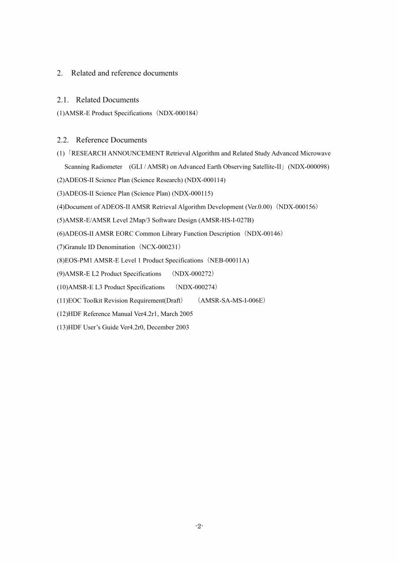
2. Related and reference documents

2.1. Related Documents (1)AMSR-E Product Specifications（NDX-000184）

2.2. Reference Documents (1)「RESEARCH ANNOUNCEMENT Retrieval Algorithm and Related Study Advanced Microwave

Scanning Radiometer (GLI / AMSR) on Advanced Earth Observing Satellite-II」(NDX-000098)

(2)ADEOS-II Science Plan (Science Research) (NDX-000114)

(3)ADEOS-II Science Plan (Science Plan) (NDX-000115)

(4)Document of ADEOS-II AMSR Retrieval Algorithm Development (Ver.0.00)（NDX-000156）

(5)AMSR-E/AMSR Level 2Map/3 Software Design (AMSR-HS-I-027B)

(6)ADEOS-II AMSR EORC Common Library Function Description（NDX-00146）

(7)Granule ID Denomination（NCX-000231）

(8)EOS-PM1 AMSR-E Level 1 Product Specifications（NEB-00011A)

(9)AMSR-E L2 Product Specifications （NDX-000272）

(10)AMSR-E L3 Product Specifications （NDX-000274）

(11)EOC Toolkit Revision Requirement(Draft） （AMSR-SA-MS-I-006E）

(12)HDF Reference Manual Ver4.2r1, March 2005

(13)HDF User’s Guide Ver4.2r0, December 2003

-2-

3. Structure of product Level 2Map product has projection of level 2 data on a map. Its data is selected from level 2 data by

specified parameters. Level2 product contains geophysical quantities, such as water vapor, cloud liquid

water, precipitation, sea surface wind speed, sea surface temperature, sea ice concentration, snow water

equivalent, and soil moisture, which are calculated from the brightness temperature. Observation point

information is also stored in it.

Level 2Map product contains two major parts the header and data. The header part is composed of

Coremeta data. Coremeta data describes the information about a product. Its detail is shown in the section

3.1.1. The calculated geophysical quantity data and position data are stored in the data part.

The structure of level 2Map product is shown in Figure 3-1.

Level 2Map Product

Geophysical Quantity Data

(SDS)Pixel

Line

Core Metadata(Header part）

（Data part）

Long. of observationpoint except 89B

(SDS)

Lat. of observationpoint except 89B

(SDS)in the scan

scan

in the scan

scan

Figure 3-1 Structure of level 2Map product.

-3-

3.1. Header part

3.1.1. Coremeta data Coremeta data contains the necessary information about the product. These items are selected from the

necessary attributes listed in the NASA ECS format, revision B.0. NASA ECS retrieves the dataset

location with attributes. The meta data is stored in the Coremeta data and its name is considered as global

attribute. Metadata in each global attribute is preserved in ASCII.

A list of coremeta data is shown in Table 3.1.1-1. The definitions of the location of the four corners and

the scene center are shown in Figure 3.1-1. As shown in the figure, the location of the four corners is the

center of each pixel, the location of the scene center is lattice point.

-4-

Table 3.1.1-1 List of Coremeta data Item Explanation Example

ShortName Product name AMSR-E-L2Map GeophysicalName Geophysical quantity name Water Vapor/Cloud liquid water/Precipitation/Sea surface

temperature/Sea surface wind speed/Sea ice concentration/Snow water equivalent/Soil moisture

VersionID ID of product version 0⎯255 SizeMBECSDataGranule Product size (Mbyte) 30(actual) LocalGranuleID Number for production

management P1AME020101001A_2MWV0Tak111EC00NWT0000

ProcessingLevelID ID of processing level L2Map ProductionDateTime Time of production (UT) 2002-1-3-T00:00:00.00Z RangeBeginningTime Time to start observing (UT) 00:00:00.00Z RangeBeginningDate Date to start observing (UT) 2002-1-3 RangeEndingTime Time to end observing (UT) 01:00:00.00Z RangeEndingDate Date to end observing (UT) 2002-1-3 PGEName Name of software (max 20 character ) PGEVersion Version of software (max 18 character ) PGEAlgorismDeveloper Name of algorism developer (max 20 character ) InputPointer Input file name P1AME020101001A_P2WV0Tak111.00 ProcessingCenter Name of data processing

center JAXA/EOC

ContactOrganizationName Organization name to contact about this product

JAXA,1401,Ohashi,Hatoyama-machi,Hiki-gun,Saitama,350-0393,JAPAN,+81-49-298-1307,orderdesk@eoc.jaxa.jp

CenterLatitude Scene center latitude 35.543 CenterLongitude Scene center longitude 123.456 UpperLeftLatitude Top left corner latitude 35.543 UpperLeftLongitude Top left corner longitude 123.456 UpperRightLatitude Top right corner latitude 35.543 UpperRightLongitude Top right corner longitude 123.456 LowerLeftLatitude Bottom left corner latitude 35.543 LowerLeftLongitude Bottom left corner longitude 123.456 LowerRightLatitude Bottom right corner latitude 35.543 LowerRightLongitude Bottom right corner longitude 123.456 StartOrbitNumber Start orbit number 100 StopOrbitNumber Stop orbit number 100 OrbitDirection Orbit direction DESCENDING EphemerisGranulePointer File name for using orbit EPHEMERIS-1 EphemerisType Type of using orbit ELMP,ELMD,GPS PlatformShortName Abbreviated name of platform Aqua SensorShortName Abbreviated name of

observing sensor AMSR-E

ECSDataModel Name of meta data model B.0 ScienceQualityFlag Flag when it calculates

geophysical quantity Blank for L1A,L1B,L1BMap

ScienceQualityFlagExplanation Explanation when it calculate geophysical quantity

Blank for L1A,L1B,L1BMap

-5-

UpperLeftLatitude/Longitude

(299,299)(0,299)

(0,0) (299,0)

UpperRightLatitude/Longitude

LowerLeftLatitude/Longitude LowerRightLatitude/Longitude

CenterLatitude/Longitude(150,0)

(151,0)

(0,150) (0,151)

Figure 3.1-1 Definition of location of four corners and scene center

-6-

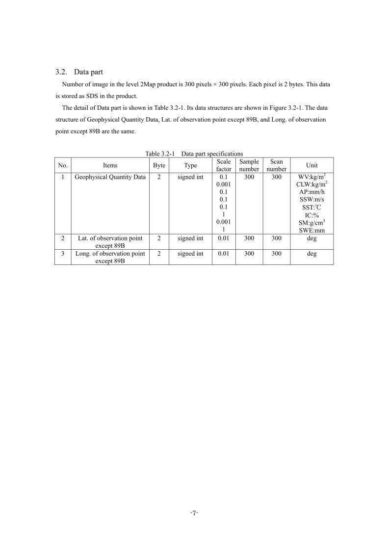
3.2. Data part Number of image in the level 2Map product is 300 pixels × 300 pixels. Each pixel is 2 bytes. This data

is stored as SDS in the product.

The detail of Data part is shown in Table 3.2-1. Its data structures are shown in Figure 3.2-1. The data

structure of Geophysical Quantity Data, Lat. of observation point except 89B, and Long. of observation

point except 89B are the same.

Table 3.2-1 Data part specifications

No. Items Byte Type Scale factor

Sample number

Scan number Unit

1 Geophysical Quantity Data 2 signed int 0.1 0.001

0.1 0.1 0.1 1

0.0011

300 300 WV:kg/m2

CLW:kg/m2

AP:mm/h SSW:m/s SST:℃ IC:%

SM:g/cm3

SWE:mm 2 Lat. of observation point

except 89B 2 signed int 0.01 300 300 deg

3 Long. of observation point except 89B

2 signed int 0.01 300 300 deg

-7-

Line No.1

Line No. 300

(0,0)

(299,0)

(299,299)

(0,299)

2byte

Figure 3.2-1 Structure of Geophysical Quantity Data, Lat. of observation point except 89B, and Long. of observation point except 89B

-8-

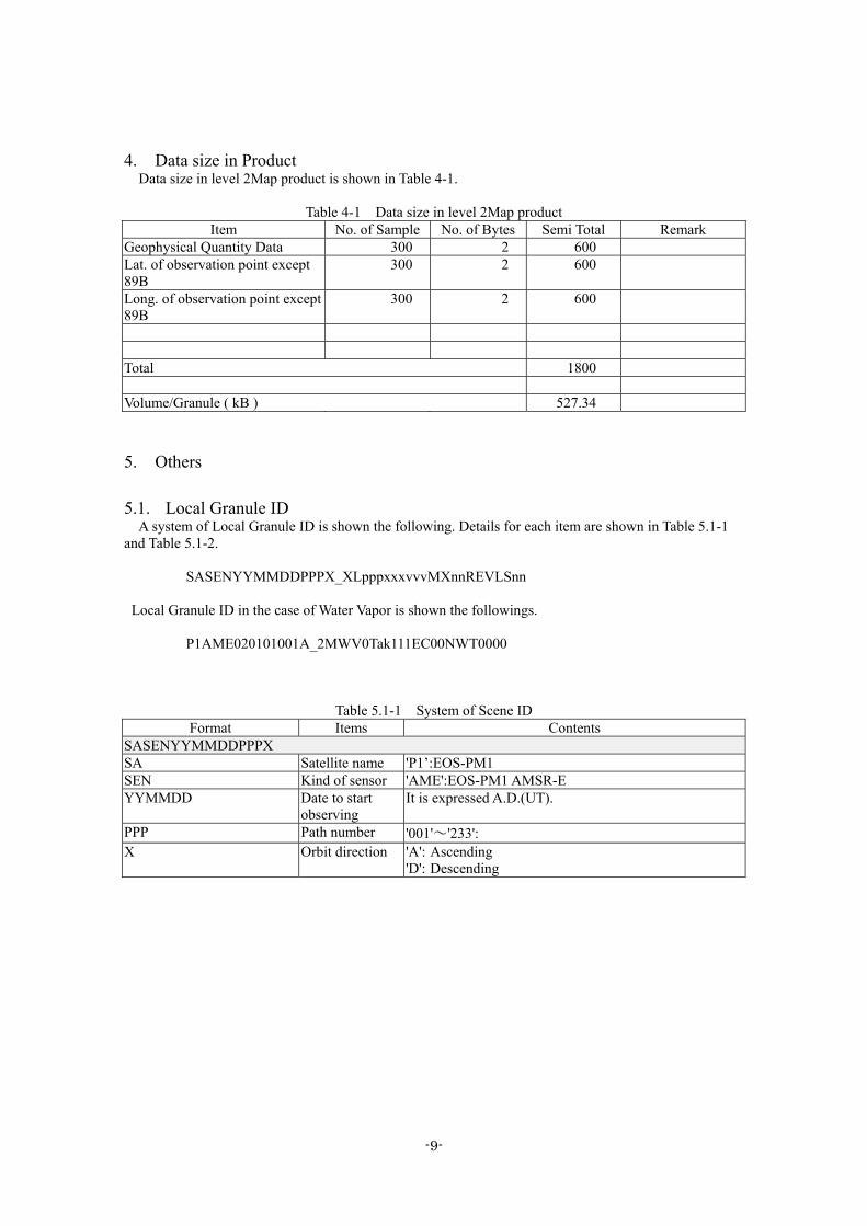
4. Data size in Product Data size in level 2Map product is shown in Table 4-1.

Table 4-1 Data size in level 2Map product

Item No. of Sample No. of Bytes Semi Total Remark Geophysical Quantity Data 300 2 600 Lat. of observation point except 89B

300 2 600

Long. of observation point except 89B

300 2 600

Total 1800

Volume/Granule ( kB ) 527.34

5. Others 5.1. Local Granule ID

A system of Local Granule ID is shown the following. Details for each item are shown in Table 5.1-1 and Table 5.1-2. SASENYYMMDDPPPX_XLpppxxxvvvMXnnREVLSnn Local Granule ID in the case of Water Vapor is shown the followings. P1AME020101001A_2MWV0Tak111EC00NWT0000

Table 5.1-1 System of Scene ID Format Items Contents

SASENYYMMDDPPPX SA Satellite name 'P1’:EOS-PM1 SEN Kind of sensor 'AME':EOS-PM1 AMSR-E YYMMDD Date to start

observing It is expressed A.D.(UT).

PPP Path number '001'～'233': X Orbit direction 'A': Ascending

'D': Descending

-9-

Table 5.1-2 System of Product ID Format Items Contents

XLpppxxxvvvMXnnREVLSnn X Kind of product 'O': Ordered product L Processing level 'M': Fixed ppp Product code 'WV0': Water Vapor

'CLW': Cloud Liquid Water 'AP0': Amount of Precipitation 'SSW': Sea Surface Wind 'SST': Sea Surface Temperature 'IC0': Ice Concentration 'SM0': Soil Moisture 'SWE': Snow Water Equivalence

xxx Name of algorism developer

'000': This item is effective only in EORC. If it is used in EOC, it is set '000'.

'Tak': Takeuchi 'Cav': Cavalieri 'Wen': Wentz 'Liu': Liu 'Pet': Petty 'Jac': Jackson 'Shi': Shibata 'Njo': Njoku 'Com': Comiso 'Pal': Paloscia 'Koi': Koike 'Kel': Kelly

vvv Algorism version It is expressed 3 characters, 'nnn'. First character, (Major version)（'0'～'9'）Last 2 characters are used as minor version('00'～'99')

M Kind of projection 'E': Equirectangular 'M': Mercator 'P': Polar stereo graphic

Xnn Base latitude 'C00': Scene center 'D00':Standard latitude 'Snn': Specified latitude (S90～N90, intervals of 5 degree)

R Interpolation 'B': Bi-liner 'N': Nearest neighbor

E Earth model 'W': WGS84 V Direction for map 'T': True North L Total movement

along longitude '0': Fixed

Snn Center latitude 'S90': South pole 'N90': North pole

-10-

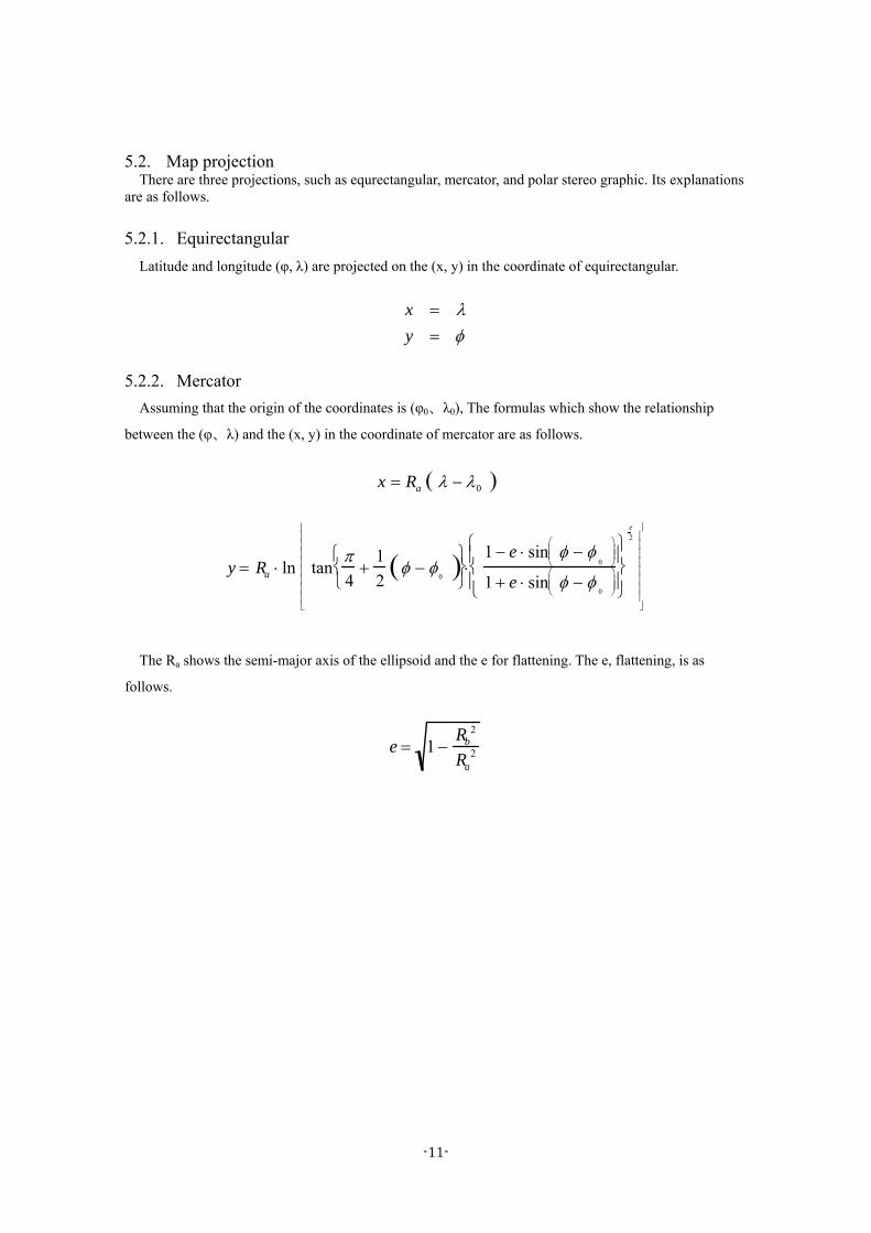
5.2. Map projection There are three projections, such as equrectangular, mercator, and polar stereo graphic. Its explanations

are as follows.

5.2.1. Equirectangular Latitude and longitude (φ, λ) are projected on the (x, y) in the coordinate of equirectangular.

x = λy = φ

5.2.2. Mercator Assuming that the origin of the coordinates is (φ0、λ0), The formulas which show the relationship

between the (φ、λ) and the (x, y) in the coordinate of mercator are as follows.

x = Ra λ − λ0( )

y = Ra ⋅ ln tanπ4

+12

φ − φ0( )⎧

⎨ ⎩

⎫ ⎬ ⎭ ⋅

1 − e ⋅ sin φ − φ0

⎛

⎝ ⎜ ⎜

⎞

⎠ ⎟ ⎟

1 + e ⋅ sin φ − φ0

⎛

⎝ ⎜ ⎜

⎞

⎠ ⎟ ⎟

⎧ ⎨ ⎪

⎩ ⎪

⎫ ⎬ ⎪

⎭ ⎪

e2

⎡

⎣

⎢ ⎢ ⎢ ⎢ ⎢ ⎢ ⎢ ⎢

⎤

⎦

⎥ ⎥ ⎥ ⎥ ⎥ ⎥ ⎥ ⎥

The Ra shows the semi-major axis of the ellipsoid and the e for flattening. The e, flattening, is as

follows.

e = 1 −Rb

2

Ra2

-11-

5.2.3. Polar stereo graphic Assuming that the coordinate of polar stereo graphic can be shown as the (X, Y) and latitude and

longitude is the (φ, λ), the relationship of each other is as follows.

（１）Calculating latitude based on the center of the earth.

Latitude based on the center of the earth, φ’, is as follows.

′ φ = tan−1 1 − e2( )tan φ{ }

（２）Calculating the position in the coordinate of polar stereo graphic

The position in the coordinate of polar stereo graphic can be calculated by the next formulas. There are

two cases in the northern hemisphere and the southern.

１）Northern hemisphere

Xm0

= − 2 Re1 − e2 cos ′ φ

1 − e2( )cos2 ′ φ + sin ′ φ sin − λ( )

Ym0

= − 2 Re1 − e2 cos ′ φ

1 − e2( )cos2 ′ φ + sin ′ φ cos − λ( )

２）Southern hemisphere

Xm0

= 2 Re1 − e2 cos ′ φ

1 − e2( )cos2 ′ φ + sin ′ φ sin λ

Ym0

= 2 Re1 − e2 cos ′ φ

1 − e2( )cos2 ′ φ + sin ′ φ cos λ

Re, e and m0 are as follows.

Re : Semi-major axis of the ellipsoid

e : Flattening 1 - f 2 m0 : Scale on the origin （1.0）

The definition of coordinates is shown in Fig. 5.2-1 and Fig. 5.2-2. In the case of the Northern

Hemisphere, a projection coordinates top is defined as the 90 west longitude, and coordinates are set up

so that it may become the 180 west longitude, the 90 east longitudes, and the zero east longitude from

-12-

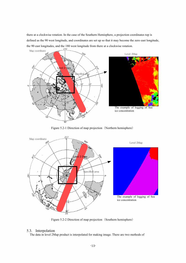
there at a clockwise rotation. In the case of the Southern Hemisphere, a projection coordinates top is

defined as the 90 west longitude, and coordinates are set up so that it may become the zero east longitude,

the 90 east longitudes, and the 180 west longitude from there at a clockwise rotation.

Level 2Map

Map coordinate

Specified area

Level 2 Data

The example of logging of Sea ice concentration

Figure 5.2-1 Direction of map projection（Northern hemisphere）

90°

Level 2Map

Map coordinate

Level 2 Data

Specified area

The example of logging of Sea ice concentration

Figure 5.2-2 Direction of map projection（Southern hemisphere）

5.3. Interpolation The data in level 2Map product is interpolated for making image. There are two methods of

-13-

interpolation, such as Nearest neighbor and Bi-linear. Explanation for its interpolation is as follows. How to interpolate is shown in Figure 5.3-1.

5.3.1. Nearest neighbor Interpolated value is the point which is the nearest observation point. Its formula is as follows.

P = Pij

i = u + 0.5[ ]j = v + 0.5[ ]

[ ] is the Gaussian symbol. It expresses the max integer value below its value.

5.3.2. Bi-linear Interpolated value is calculated from four points which are near the observation point. Its formula is as

follows.

P = i + 1( ) − u{ } j + 1( )− v{ }Pi , j + i + 1( ) − u{ } v − j( ) Pi, j +1

+ u − i( ) j +1( ) − v{ }Pi +1, j + u − i( ) v − j( ) Pi +1, j +1

N N 法

Pi,j Pi+1,j

Pi,j+1 Pi+1,j+1

P(u,v)

Pi,jPi+1,j

Pi,j+1 Pi+1,j+1

P(u,v)

u

v

B L法

:　内

Nearest neighbor

挿したい点Calculated point

:　観測点Observation point

Bi-linear

-14-

Figure 5.3-1 How to interpolate

-15-

5.4. Dummy data The dummy data (data other than the amount of geophysics) in level 2Map is as follows.

* -9999 : When there is no geophysical data within observation swath

This value is set up when computing neither the case where the amount of geophysics is incomputable (a packet loss, the abnormalities in brightness temperature of level 1B, the amount calculation error of geophysics, etc.) , nor the amount of geophysics (This case is based on conditions peculiar to the amount of physics. For example, in the case of the amount of geophysics for marine [, such as SST, ], the area of land does not compute the amount of geophysics.).

* -8888 : The area besides observation swath The example of a picture image of Sea ice concentration level 2Map is shown in Figure 5.4-1. Since it is outside observation swath, "-8888" is set up.

Since the amount of geophysics was not computed by level 2 processing, -9999 is set up.

Geophysical Quantity Data

Figure 5.4-1 The example of a picture image of Sea ice concentration level 2Map

-16-

6. Explanation about data Explanation for each data is shown in next section. Each item in its explanation is described the

followings. HDF_MODEL：HDF model to put each data in the file. In the case of standard product, the data has "scientific data sets", "Vdata" and "global attribute". Most of data elements are set as scientific data sets in it. ARRAY_DIMENSION：Data size of each dimension if data type is array dimension(in the case of nominal). STORAGE_TYPE：Type of data element. There are "int 8", "int16", "int32", "unsigned integer8","unsigned integer32", "float32", "float64". NUMBER_OF_BYTE：Number of byte to preserve the data element. UNIT：Data unit. For example, there are "deg", "count2", ”Kelvin”, and so on. MINIMUM_VALUE：Minimum value of data element. MAXIMUM_VALUE：Maximum value of data element. SCALE_FACTOR：Standard product has some elements which is changed float into integer for interchangeable among the machines and preserved(for example, geophysical quantity etc.). That's why it is necessary to multiply the stored data by scale_factor for use. The scale_factor is used when the data, which is changed float into integer is put it back. （For example, when the sea surface temperature is 18.36℃, it is stored as 1836 and scale_factor becomes 0.01.）

6.1. Explanation for each data Explanations for each data are as follows. （１）Geophysical Quantity Data

HDF_MODEL : SDS ARRAY_DIMENSION :300×300 STORAGE_TYPE : Signed int 16 NUMBER_OF_BYTE : 2 UNIT : kg/m2 (WV,CLW) / mm (SWE) / mm/h (AP) / m/s (SSW) / ℃ (SST) / % (IC) g/cm3 (SM) MINIMUM_VALUE : 0 (WV) / 0 (CLW) / 0 (AP) / 0 (SSW) / -2 (SST) / 0 (IC) / 0 (SM) 0 (SWE) MAXIMUM_VALUE : 70 (WV) / 1.0 (CLW) / 100 (AP) / 30 (SSW) / 35 (SST) / 100 (IC) TBD (SM) / 10000 (SWE) SCALE_FACTOR : 0.1 (WV) / 0.001 (CLW) / 0.1 (AP) / 0.1 (SSW) / 0.1 (SST) / 1 (IC) 0.001 (SM) / 1 (SWE)

（２）Lat. of observation point except 89B Latitude of observation points corresponding to Geophysical Quantity Data explained above is stored.

North latitude is expressed as 0 to 90 degrees, while south latitude is expressed as -90 to 0 degrees. HDF_MODEL : SDS

-17-

ARRAY_DIMENSION : 300×300 STORAGE_TYPE : signed int 16 NUMBER_OF_BYTE : 2 UNIT : deg MINIMUM_VALUE : -90 MAXIMUM_VALUE : 90 SCALE_FACTOR : 0.01

（３）Long. of observation point except 89B

Longitude of observation points corresponding to Geophysical Quantity Data explained above is stored. East longitude is expressed as 0 to 180 degrees, while west longitude is express as -180 to 0 degrees. HDF_MODEL : SDS ARRAY_DIMENSION : 300×300 STORAGE_TYPE : signed int 16 NUMBER_OF_BYTE : 2 UNIT : deg MINIMUM_VALUE : -180 MAXIMUM_VALUE : 180 SCALE_FACTOR : 0.01

-18-

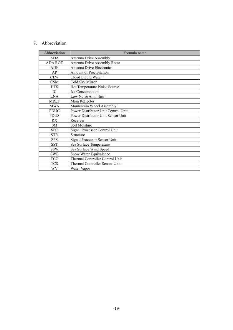
7. Abbreviation

Abbreviation Formula name ADA Antenna Drive Assembly

ADA ROT Antenna Drive Assembly Rotor ADE Antenna Drive Electronics AP Amount of Precipitation

CLW Cloud Liquid Water CSM Cold Sky Mirror HTS Hot Temperature Noise Source IC Ice Concentration

LNA Low Noise Amplifier MREF Main Reflector MWA Momentum Wheel Assembly PDUC Power Distributor Unit Control Unit PDUS Power Distributor Unit Sensor Unit

RX Receiver SM Soil Moisture SPC Signal Processor Control Unit STR Structure SPS Signal Processor Sensor Unit SST Sea Surface Temperature SSW Sea Surface Wind Speed SWE Snow Water Equivalence TCC Thermal Controller Control Unit TCS Thermal Controller Sensor Unit WV Water Vapor

-19-