Appendix 6-2: HFSS 3D Boundary Conditions - · PDF fileAppendix 6-2: HFSS 3D Boundary...

Release 2015.0 April 16, 2015 1 © 2015 ANSYS, Inc.

2015.0 Release

Appendix 6-2: HFSS 3D Boundary Conditions

Introduction to ANSYS HFSS


HFSS Design Setup

Geometry Materials Boundaries

Excitations

Solve Setup

GUI

Solve HPC

Mesh

Design Setup


Boundary Conditions

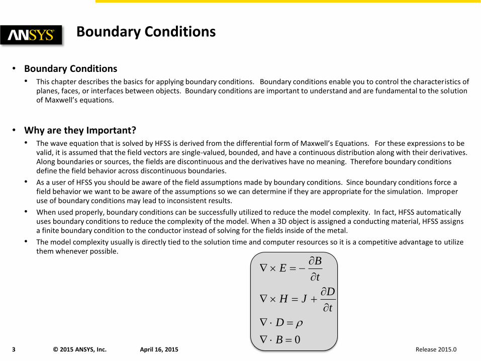
• Boundary Conditions • This chapter describes the basics for applying boundary conditions. Boundary conditions enable you to control the characteristics of

planes, faces, or interfaces between objects. Boundary conditions are important to understand and are fundamental to the solution of Maxwell’s equations.

• Why are they Important? • The wave equation that is solved by HFSS is derived from the differential form of Maxwell’s Equations. For these expressions to be

valid, it is assumed that the field vectors are single-valued, bounded, and have a continuous distribution along with their derivatives. Along boundaries or sources, the fields are discontinuous and the derivatives have no meaning. Therefore boundary conditions define the field behavior across discontinuous boundaries.

• As a user of HFSS you should be aware of the field assumptions made by boundary conditions. Since boundary conditions force a field behavior we want to be aware of the assumptions so we can determine if they are appropriate for the simulation. Improper use of boundary conditions may lead to inconsistent results.

• When used properly, boundary conditions can be successfully utilized to reduce the model complexity. In fact, HFSS automatically uses boundary conditions to reduce the complexity of the model. When a 3D object is assigned a conducting material, HFSS assigns a finite boundary condition to the conductor instead of solving for the fields inside of the metal.

• The model complexity usually is directly tied to the solution time and computer resources so it is a competitive advantage to utilize them whenever possible.

0

B

D

t

DJH

t

BE


Common Boundary Conditions

• Common Boundary Conditions • There are three types of boundary conditions. The first two are largely the users responsibility to define them or ensure that they

are defined correctly. The material boundary conditions are transparent to the user.

– Excitations

• Wave Ports (External)

• Lumped Ports (Internal)

– Surface Approximations

• Symmetry Planes

• Perfect Electric or Magnetic Surfaces

• Radiation (absorbing) boundary surface

– Perfectly matched layer (PML)

• Strictly not boundary condition, but effectively behaves like one

– Finite Element-Boundary Integral (FEBI)

• Background or Outer Surface

• Finite conductivity surface

• Impedance surface

– Layered impedance

– Lumped RLC boundary

• Master/slave (linked or periodic) boundaries

– Screening impedance

– Material Properties

• Boundary between two dielectrics

• Finite Conductivity of a conductor


Boundary Condition Precedence

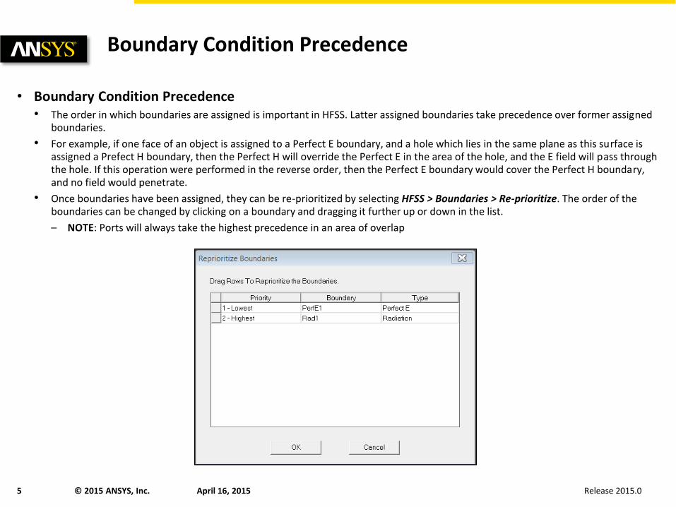
• Boundary Condition Precedence • The order in which boundaries are assigned is important in HFSS. Latter assigned boundaries take precedence over former assigned

boundaries.

• For example, if one face of an object is assigned to a Perfect E boundary, and a hole which lies in the same plane as this surface is assigned a Prefect H boundary, then the Perfect H will override the Perfect E in the area of the hole, and the E field will pass through the hole. If this operation were performed in the reverse order, then the Perfect E boundary would cover the Perfect H boundary, and no field would penetrate.

• Once boundaries have been assigned, they can be re-prioritized by selecting HFSS > Boundaries > Re-prioritize. The order of the boundaries can be changed by clicking on a boundary and dragging it further up or down in the list.

– NOTE: Ports will always take the highest precedence in an area of overlap


Background or Outer Surface

• How the Background Affects a Structure • The background is a hidden region that is automatically defined by HFSS. The background surrounds the geometric model and fills

any space that is not occupied by an object. Any object surface that touches the background is automatically defined to be a Perfect E boundary and given the boundary name outer. You can think of your structure as being encased with a thin, perfect conductor.

• If it is necessary, you can change a surface that is exposed to the background to have properties that are different from outer:

– To model losses in a surface, you can redefine the surface to be either a Finite Conductivity or Impedance boundary.

– To model a surface to allow waves to radiate infinitely far into space, redefine the surface to be radiation boundary.

• The background can affect how you make material assignments. For example, if you are modeling a simple air-filled rectangular waveguide, you can create a single object in the shape of the waveguide and define it to have the characteristics of air. The surface of the waveguide is automatically assumed to be a perfect conductor and given the boundary condition outer, or you can change it to a lossy conductor.


Technical Definitions

• Technical Definition of Boundary Conditions • Perfect E – Perfect E is a perfect electrical conductor (PEC), also referred to as a perfect conductor.

– Forces E-field perpendicular to surface

– Used to model lossless metal surfaces, ground planes, cavity walls, etc.

– Can be assigned to 2D or 3D objects

– There are also two automatic Perfect E assignments:

• Any object surface that touches the background is automatically defined to be a Perfect E boundary and given the boundary condition name outer.

• Any object that is assigned the material pec (Perfect Electric Conductor) is automatically assigned the boundary condition Perfect E to its surface and given the boundary condition name smetal.

• Perfect H – Perfect H is a perfect magnetic conductor.

– Forces H-field perpendicular to surface and E-field tangential

– Does not exist in real world

– Natural – for a Perfect H boundary that overlaps with a perfect E boundary, this reverts the selected area to its original material, erasing the Perfect E boundary condition. It does not affect any material assignments. It can be used, for example, to model a cut-out in a ground plane for a coax feed.

Perfect E Boundary

E-field Perpendicular to surface

Perfect H Boundary

E-field Parallel to surface



• Surface Loss Modeling • Finite Conductivity –A Finite Conductivity boundary enables you to define the surface of an object as a lossy (imperfect) conductor.

HFSS applies this boundary for lossy metal materials. To model a lossy surface, you provide loss in Siemens/meter and permeability parameters. Loss is calculated as a function of frequency. It is only valid for good conductors. Forces the tangential E-Field equal to Zs(n x Htan). The surface impedance (Zs) is equal to, (1+j)/(), where:

– is the skin depth, (2/())0.5 of the conductor being modeled, is the frequency of the excitation wave, is the conductivity of the conductor, is the permeability of the conductor

• Impedance – a resistive surface that calculates the field behavior and losses using analytical formulas. Forces the tangential E-Field equal to Zs(n x Htan). The surface impedance is equal to Rs + jXs, where:

– Rs is the resistance in ohms/square, Xs is the reactance in ohms/square

• Layered Impedance – Multiple thin layers in a structure can be modeled as an impedance surface. See the Online Help for additional information on how to use the Layered Impedance boundary.

• Lumped RLC – a parallel combination of lumped resistor, inductor, and/or capacitor surface. The simulation is similar to the Impedance boundary, but the software calculate the ohms/square using the user supplied R, L, C values.

• Infinite Ground Plane – Generally, the ground plane is treated as an infinite, Perfect E, Finite Conductivity, or Impedance boundary condition. If radiation boundaries are used in a structure, the ground plane acts as a shield for far-field energy, preventing waves from propagating past the ground plane. To simulate the effect of an infinite ground plane, check the Infinite ground plane box when defining a Perfect E, Finite Conductivity, or Impedance boundary condition.

– NOTE: Enabling the Infinite Ground Plane approximation ONLY affects post-processed far-field radiation patterns. It will not change the current flowing on the ground plane.


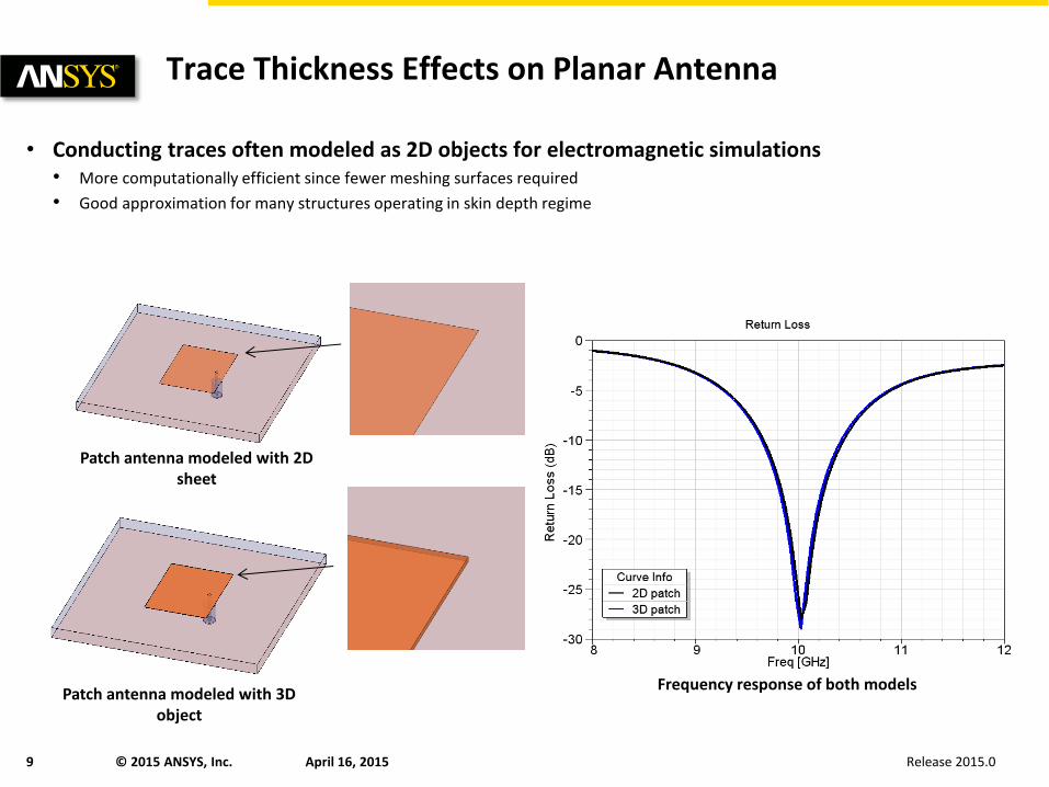
Trace Thickness Effects on Planar Antenna

• Conducting traces often modeled as 2D objects for electromagnetic simulations • More computationally efficient since fewer meshing surfaces required

• Good approximation for many structures operating in skin depth regime

Patch antenna modeled with 2D sheet

Patch antenna modeled with 3D object

Frequency response of both models


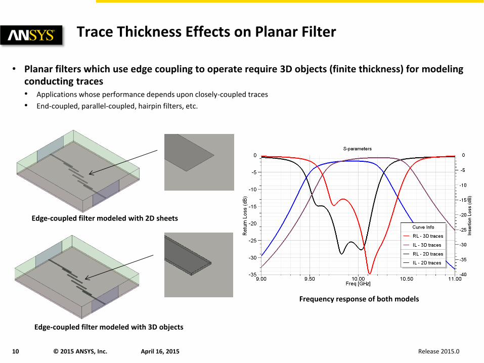
Trace Thickness Effects on Planar Filter

• Planar filters which use edge coupling to operate require 3D objects (finite thickness) for modeling conducting traces • Applications whose performance depends upon closely-coupled traces

• End-coupled, parallel-coupled, hairpin filters, etc.

Edge-coupled filter modeled with 2D sheets

Edge-coupled filter modeled with 3D objects

Frequency response of both models



• Radiating Boundary Conditions • Radiation boundaries, also referred to as absorbing boundaries, enable you to model a surface as electrically open: waves can then

radiate out of the structure and toward the radiation boundary. The system absorbs the wave at the radiation boundary, essentially ballooning the boundary infinitely far away from the structure and into space. Radiation boundaries may also be placed relatively close to a structure and can be arbitrarily shaped. This condition eliminates the need for a spherical boundary. For structures that include radiation boundaries, calculated S-parameters include the effects of radiation loss. When a radiation boundary is included in a structure, far-field calculations are performed as part of the simulation.

• Perfectly Matched Layers (PMLs) are fictitious materials that fully absorb the electromagnetic fields acting upon them.

– There are two types of PML applications: “free space termination” and “reflection-free termination” of guided waves.

• In free space termination, all PML objects must be included in a surface that radiates into free space equally in every direction. PMLs can be superior to radiation boundaries in this case because PMLs enable radiation surfaces to be located closer to radiating objects, reducing the problem domain. Any homogenous isotropic material, including lossy materials such as ocean water, can surround the model.

• In reflection-free termination of guided waves, the structure continues uniformly to infinity. The termination surface of the structure radiates in the direction in which the wave is guided. Reflection-free PMLs are superior to free space or radiation boundary terminations in this kind of application. Reflection-free PMLs are also superior for simulating phased array antennas because the antenna radiates in a certain direction.

• Finite Element Boundary Integral (FEBI) is an alternative to Radiation and PML boundaries for radiating designs. The FEBI boundary is a hybrid FEM (Volume) and IE solver (Radiating Surface). FEBI is a reflection-less boundary that can be applied to arbitrarily shaped volumes. Requires an HFSS-IE license.


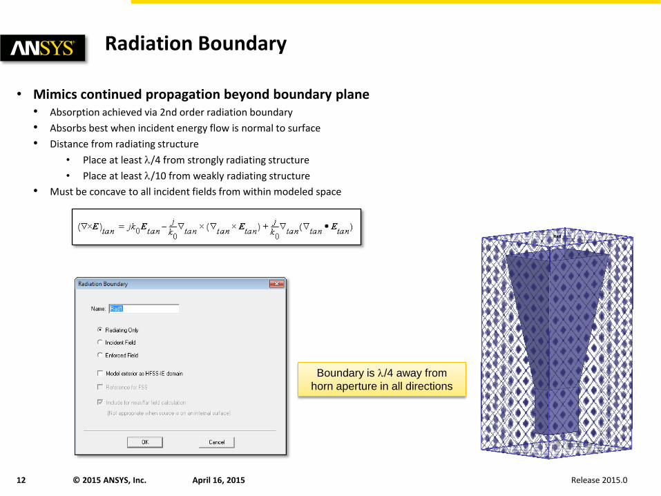
Radiation Boundary

• Mimics continued propagation beyond boundary plane • Absorption achieved via 2nd order radiation boundary

• Absorbs best when incident energy flow is normal to surface

• Distance from radiating structure

• Place at least /4 from strongly radiating structure

• Place at least /10 from weakly radiating structure

• Must be concave to all incident fields from within modeled space

Boundary is /4 away from

horn aperture in all directions


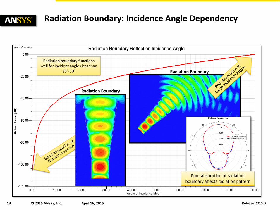
Radiation Boundary: Incidence Angle Dependency

Radiation boundary functions well for incident angles less than

25°-30°

Radiation Boundary

Radiation Boundary

Poor absorption of radiation boundary affects radiation pattern


Impact of Distance to ABC

• Example probe-fed circular patch • Varied distance between absorbing boundary condition (ABC) and antenna

– λ /20, λ /10, λ /8, λ /4, λ /2, 3 λ /4, λ

• Examined impact on return loss and gain

/4 and cases within 13 MHz of each other (0.1%)

0.2 dB variation


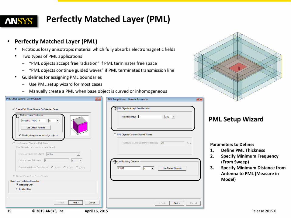
Perfectly Matched Layer (PML)

• Perfectly Matched Layer (PML) • Fictitious lossy anisotropic material which fully absorbs electromagnetic fields

• Two types of PML applications

– “PML objects accept free radiation” if PML terminates free space

– “PML objects continue guided waves” if PML terminates transmission line

• Guidelines for assigning PML boundaries

– Use PML setup wizard for most cases

– Manually create a PML when base object is curved or inhomogeneous

PML Setup Wizard

Parameters to Define: 1. Define PML Thickness 2. Specify Minimum Frequency

(From Sweep) 3. Specify Minimum Distance from

Antenna to PML (Measure in Model)

1.

2.

3.


PML: Incidence Angle Dependency

PML functions well for

incident angles less than

65°-70° Better absorption leads to better consistency in the patterns

PML

PML


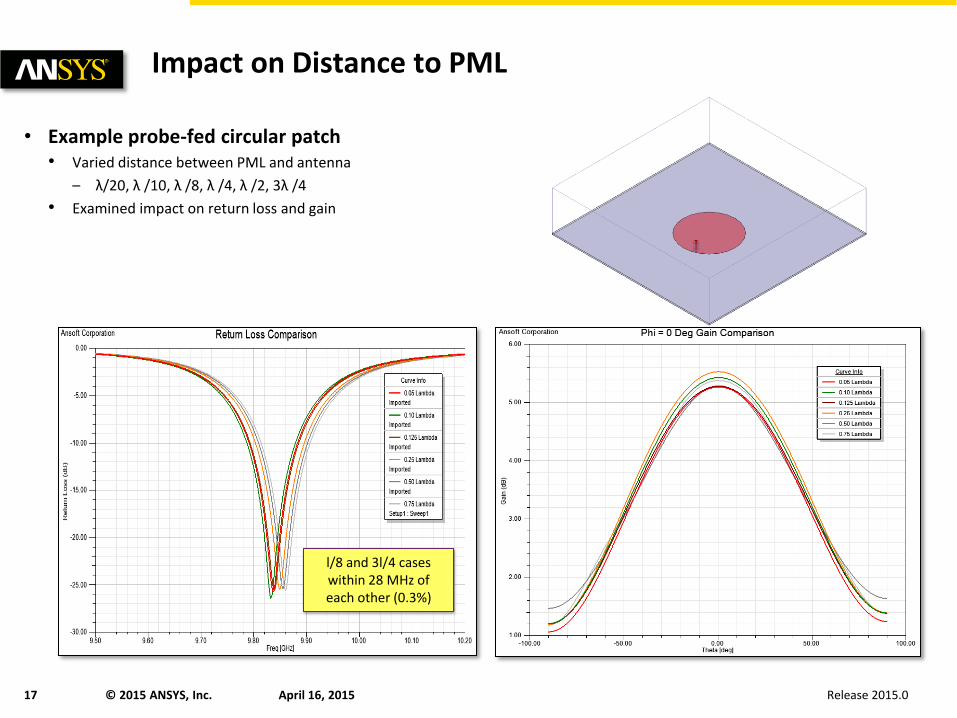
Impact on Distance to PML

• Example probe-fed circular patch • Varied distance between PML and antenna

– λ/20, λ /10, λ /8, λ /4, λ /2, 3λ /4

• Examined impact on return loss and gain

l/8 and 3l/4 cases within 28 MHz of each other (0.3%)


Finite Element – Boundary Integral

• FEBI • Mesh truncation of infinite free space into a finite computational domain

• Alternative to Radiation or PML

• Hybrid solution of FEM and IE

– IE solution on outer faces

– FEM solution inside of volume

• FE-BI Advantages

– Arbitrary shaped boundary

• Conformal and discontinuous to minimize solution volume

– Reflection-less boundary condition

• High accuracy for radiating and scattering problems

– No theoretical minimum distance from radiator

• Reduce simulation volume and simplify problem setup

FEM Solution

in Volume

IE Solution

on Outer Surface

Fields at outer surface

Iterate

Free space (No Solution Volume)

FE-BI

Arbitrary shape


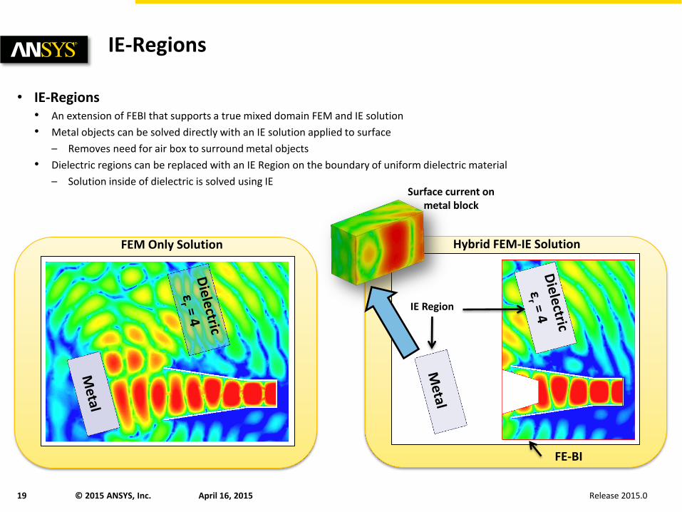
IE-Regions

• IE-Regions • An extension of FEBI that supports a true mixed domain FEM and IE solution

• Metal objects can be solved directly with an IE solution applied to surface

– Removes need for air box to surround metal objects

• Dielectric regions can be replaced with an IE Region on the boundary of uniform dielectric material

– Solution inside of dielectric is solved using IE

FE-BI

IE Region

Surface current on metal block

FEM Only Solution Hybrid FEM-IE Solution


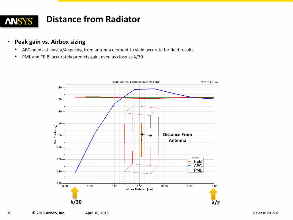
Distance from Radiator

• Peak gain vs. Airbox sizing • ABC needs at least λ/4 spacing from antenna element to yield accurate far field results

• PML and FE-BI accurately predicts gain, even as close as λ/30

Distance From Antenna

λ/30 λ/2



• Technical Definition of Boundary Conditions (Continued) • Symmetry - represent perfect E or perfect H planes of symmetry. Symmetry boundaries enable you to model only part of a

structure, which reduces the size or complexity of your design, thereby shortening the solution time. Symmetry boundaries, as opposed to a simple Perfect E or H plane, should be used when the plane cuts across a port. In this instance, the port has a different amount of power, voltage, and current associated with it, and thus a different impedance. To make a port with a symmetry plane look like a full-sized port, you must use the Impedance Multiplier in the boundary wizard.

– For a single Symmetry H boundary, the Impedance Multiplier is 0.5.

– For a single Symmetry E boundary, the Impedance Multiplier is 2.

– Other considerations for a Symmetry boundary condition:

• A plane of symmetry must be exposed to the background.

• A plane of symmetry must not cut through an object drawn in the 3D Modeler window.

• A plane of symmetry must be defined on a planar surface.

• Only three orthogonal symmetry planes can be defined in a problem

Conductive edges on all four sides

Perfect E Symmetry (bottom)

Perfect H Symmetry (left side)

Waveguide contains symmetric propagating mode which could be modeled using half the volume vertically or horizontally.


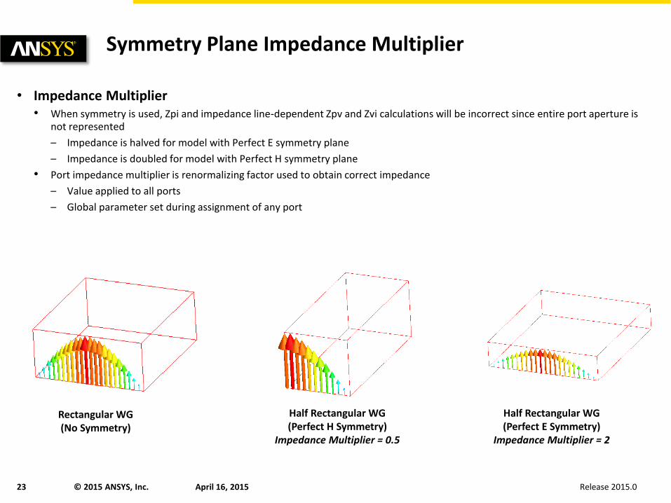
Symmetry Plane Impedance Multiplier

• Impedance Multiplier • When symmetry is used, Zpi and impedance line-dependent Zpv and Zvi calculations will be incorrect since entire port aperture is

not represented

– Impedance is halved for model with Perfect E symmetry plane

– Impedance is doubled for model with Perfect H symmetry plane

• Port impedance multiplier is renormalizing factor used to obtain correct impedance

– Value applied to all ports

– Global parameter set during assignment of any port

Rectangular WG (No Symmetry)

Half Rectangular WG (Perfect E Symmetry)

Impedance Multiplier = 2

Half Rectangular WG (Perfect H Symmetry)

Impedance Multiplier = 0.5


Perfect E Symmetry (top)

Perfect H Symmetry (right side)

TE20 mode in full model Properly represented with

Perfect E symmetry Mode cannot occur with

Perfect H symmetry

Symmetry Plane Mode Implications

• Field Symmetry • Geometric symmetry does not necessarily imply field symmetry for higher-order modes

• Symmetry boundaries can act as mode filters

– Next higher propagating waveguide mode is not symmetric about vertical center plane of waveguide

– Therefore one symmetry case is valid while the other is not

• Use caution when using symmetry planes to assure that real behavior is not filtered out by boundary conditions



• Technical Definition of Boundary Conditions (Continued) • Master / Slave - Master and slave boundaries enable you to model planes of periodicity where the E-field on one surface matches

the E-field on another to within a phase difference. They force the E-field at each point on the slave boundary match the E-field to within a phase difference at each corresponding point on the master boundary. They are useful for simulating devices such as infinite arrays. Some considerations for Master/Slave boundaries:

– They can only be assigned to planar surfaces.

– The geometry of the surface on one boundary must match the geometry on the surface of the other boundary.

• Screening Impedance - Used to efficiently represent periodic screens or grids with impedance boundary condition


Master/Slave Boundaries

• Master/Slave Boundaries • Used to model unit cell of periodic structure

– Also referred to as linked or periodic boundaries

• Master and slave boundaries are always paired

– Fields on master surface are mapped to slave surface with a phase shift

– Phase shift specified either as absolute phase value or using scan angle

• Constraints

– Master and slave surfaces must be identical in shape and size

– Coordinate systems must be created to identify point-to-point correspondence

• Parameters

– Master/slave pairing

– UV coordinate systems

– Phase shift method

Unit Cell Model of Waveguide Array

WG Port (bottom)

Ground Plane

Master Boundary Slave

Boundary

V-axis

U-axis


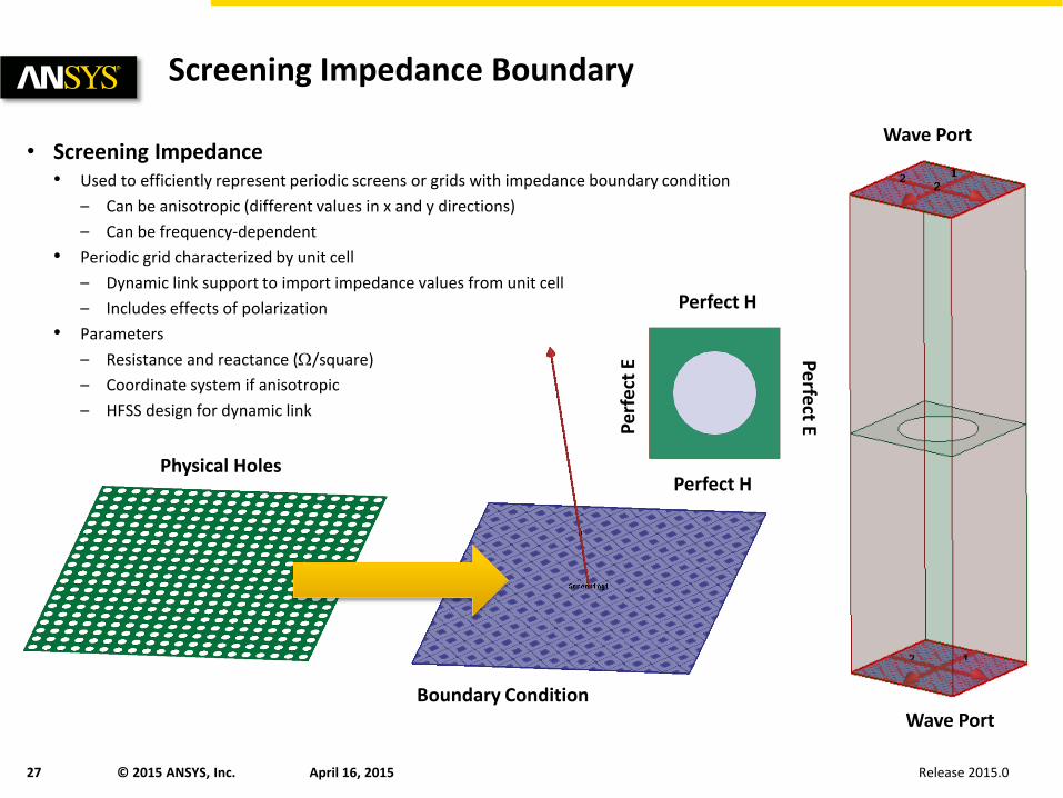
Screening Impedance Boundary

• Screening Impedance • Used to efficiently represent periodic screens or grids with impedance boundary condition

– Can be anisotropic (different values in x and y directions)

– Can be frequency-dependent

• Periodic grid characterized by unit cell

– Dynamic link support to import impedance values from unit cell

– Includes effects of polarization

• Parameters

– Resistance and reactance (/square)

– Coordinate system if anisotropic

– HFSS design for dynamic link

Pe

rfe

ct E

Pe

rfect E

Perfect H

Perfect H

Wave Port

Wave Port

Physical Holes

Boundary Condition

Date post:	18-Feb-2018
Category:	Documents
Upload:	trankhanh
View:	499 times
Download:	50 times

Appendix 6-2: HFSS 3D Boundary Conditions - · PDF fileAppendix 6-2: HFSS 3D Boundary...

Documents