Appendix 8B Sacramento River Ecological Flows Line items and numbers identified or noted as “No Action Alternative” represent the “Existing Conditions/No Project/No Action Condition” (described in Chapter 2 Alternatives Analysis). Table numbering may not be consecutive for all appendixes.
Transcript
Appendix 8B Sacramento River Ecological Flows
Line items and numbers identified or noted as “No Action Alternative” represent the “Existing Conditions/No Project/No Action Condition” (described in Chapter 2 Alternatives Analysis). Table numbering may not be consecutive for all appendixes.
This page intentionally left blank.
NODOS AnalysisCorrected Literature Cited
This page intentionally left blank.
Analysis of the North-of-the-Delta
Offstream Storage Investigation
Prepared for
Statewide Infrastructure Investigations Branch
Prepared by
Sacramento River Project
500 Main St.
Chico, CA 95928
and
600 - 2695 Granville St.
Vancouver, BC
Canada V6H 3H4
October 4, 2012
Citation: The Nature Conservancy and ESSA Technologies Ltd. 2012. SacEFT Analysis of the North-of-the-Delta
Offstream Storage Investigation. The Nature Conservancy, Chico, CA. 73pp + appendices.
Any inquiries regarding this report should be directed to:
List of Tables ................................................................................................................................................................ ii
List of Figures ............................................................................................................................................................. iv
5. Literature Cited .................................................................................................................................................. 68
6. Further Reading ................................................................................................................................................. 70
6. Appendix A – Inverse Correlation between Juvenile Stranding and Juvenile Rearing in SacEFT ............ 74
Appendix B – Indicator Thresholds and Rating System ........................................................................................ 79
Appendix C – Additional Chinook Reports............................................................................................................. 86
C.2 Fall Chinook ........................................................................................................................................... 93
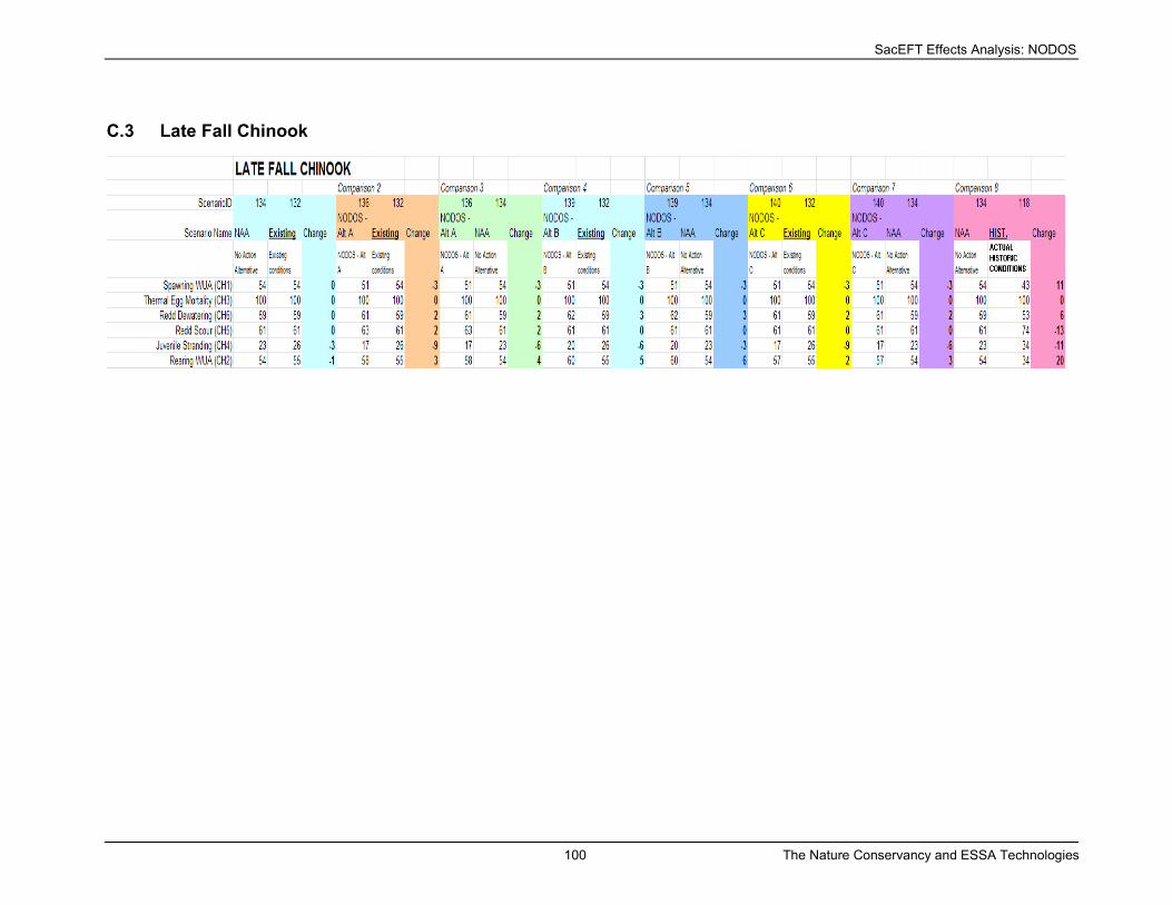
C.3 Late Fall Chinook ................................................................................................................................. 100
C.4 Spring Chinook .................................................................................................................................... 107
Table 2-B: Spatial location and extent of physical datasets, linked models and performance measures for
the non-salmonid focal species. Performance measures (PMs) for the species are summarized in
Table 2-A. Vertical bars denote PMs that are simulated for river segments; dots denote those
that are simulated (measured in the case of gauges) at points along the river. Q = river
discharge. T = water temperature. Annotation details are listed in Table 2-D. ...................................... 18
Table 2-C: Spatial location and extent of physical datasets, linked models and performance measures for
the salmonid focal species. Performance measures (PMs) for the species are summarized in
Table 2-A. Vertical bars denote PMs that are simulated for river segments; dots denote those
that are simulated (measured in the case of gauges) at points along the river. Q = river
discharge. T = water temperature. Annotation details are listed in Table 2-D. ...................................... 19
Table 2-D: Annotations for Table 2-B and Table 2-C. ............................................................................................. 20
Table 2-E: Summary of the life-history timing information relevant to the SacEFT focal species. Only those
performance measures requiring information on life history timing are included here.
Abbreviations of performance measures (PMs) are described in Table 2-A. Time intervals
marked with heavy color denote periods of greater importance to focal species. In the case of
the spawning PMs (CS-1), heavily shaded regions denote for each salmonid run-type/species the
period between the 25th and 75
th percentile, when half the spawning takes place. In the case of
the other salmonid PMs, the heavily shaded regions denote the period between the 25th and 75
th
percentile of the population are present. Specific timing of CS-2, 3, 4, 5, 6 depends on ambient
water temperature and varies with discharge scenario and year. Juvenile residency is defined by
a fixed 90 day period following emergence for Chinook and a 365 day period for steelhead. This
table is based on SALMOD (Bartholow and Heasley 2006, ultimately Vogel and Marine 1991).
Salmonid timing values shown here are typical and may shift by as much as five days earlier or
later, depending on year and reach. Timing values for green sturgeon, cottonwood and bank
swallow are based on workshop discussions, and all values are under user control. ............................. 21
Table 2-F: Potential revetment removal sites on the middle Sacramento River. Sites 2-6 define the “rip rap
removal” scenario in SacEFT. For details see Larsen (2007). ............................................................... 24
Table 3-A: Rank order of preferred NODOS alternative by focal species or group based on synthesis results
in Table 3-B. .......................................................................................................................................... 33
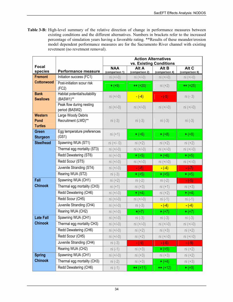
Table 3-B: High-level summary of the relative direction of change in performance measures between
existing conditions and the different alternatives. Numbers in brackets refer to the increased
percentage of simulation years having a favorable rating. **Results of these meander/erosion
model dependent performance measures are for the Sacramento River channel with existing
revetment (no revetment removal). ........................................................................................................ 34
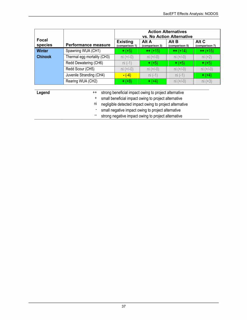
Table 3-C: High-level summary of the relative direction of change in performance measures between the
No Action Alternative and the different alternatives. Numbers in brackets refer to the increased
percentage of simulation years having a favorable rating. **Results of these meander/erosion
model dependent performance measures are for the Sacramento River channel with existing
revetment (no revetment removal). ........................................................................................................ 36
Table 3-D: High-level summary of the relative direction of change in performance measures between the
No Action Alternative (which reflects 2030 conditions, constraints and operations) and
historical flows. Numbers in brackets refer to the increased percentage of simulation years
having a favorable rating. **Results of these meander/erosion model dependent performance
measures are for the Sacramento River channel with existing revetment (no revetment removal). ....... 38
SacEFT Effects Analysis: NODOS
iii
SacEFT Effects Analysis: NODOS
iv
List of Figures
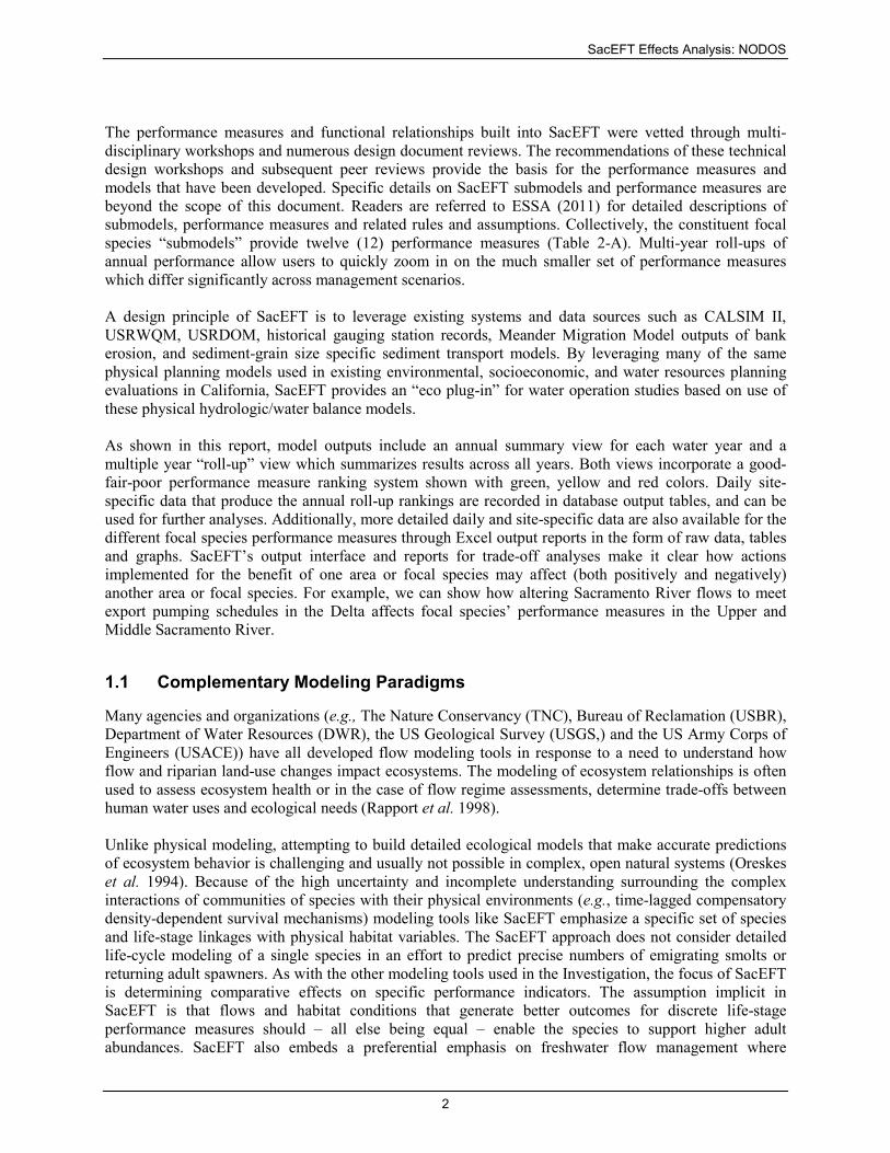
Figure 1.1: Attributes of alternative ecological flow assessment tools showing placement of the Sacramento
River Ecological Flows Tool (SacEFT; ESSA (2011)). IHA = Indicators of Hydrologic
Alteration (Mathews and Richter 2007). HAT = Hydrologic Assessment Tool (Kennen et al.
2009). RVA = Range of Variability Analysis (Mathews and Richter 2007). HEC-EFM =
Hydrologic Engineering Center Ecosystem Functions Model (USACE 2002). IOS = Winter-run
Chinook IOS/DPM. SALMOD = Salmonid Population Model (Bartholow et al. 2002). ........................ 4
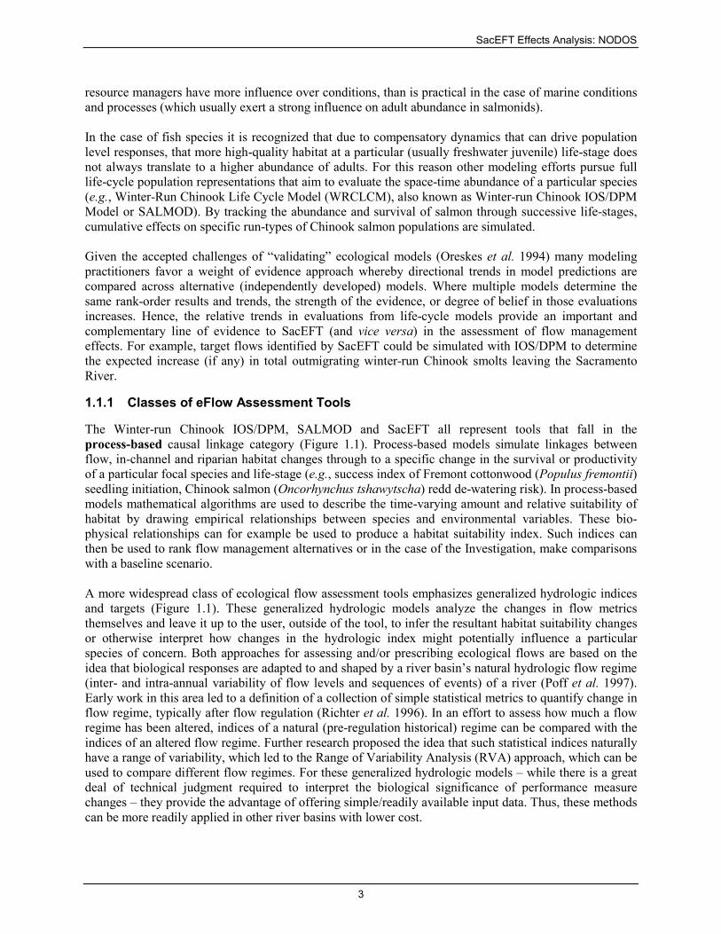
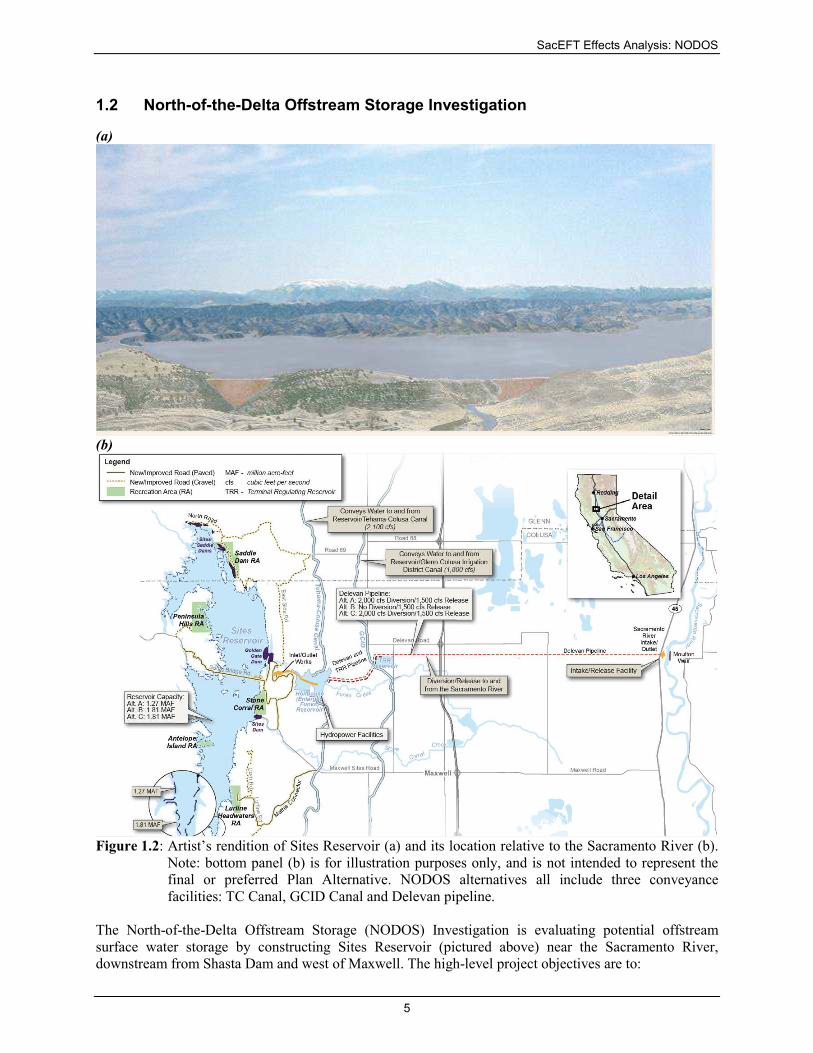
Figure 1.2: Artist’s rendition of Sites Reservoir (a) and its location relative to the Sacramento River (b).
Note: bottom panel (b) is for illustration purposes only, and is not intended to represent the final
or preferred Plan Alternative. NODOS alternatives all include three conveyance facilities: TC
Canal, GCID Canal and Delevan pipeline. ............................................................................................... 5
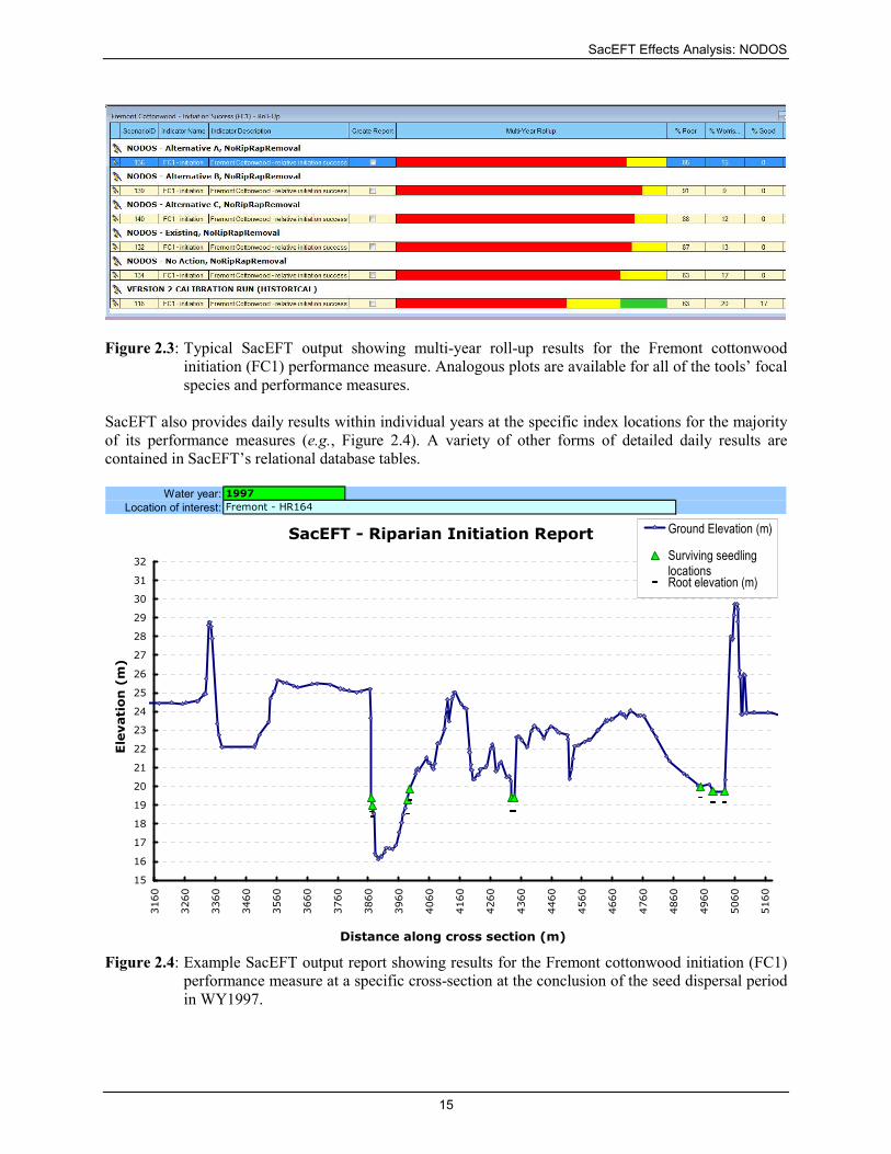
Figure 2.1: Typical SacEFT output showing annual roll-up results for the Fremont cottonwood initiation
(FC1) performance measure. Analogous plots are available for all of the tools’ focal species and
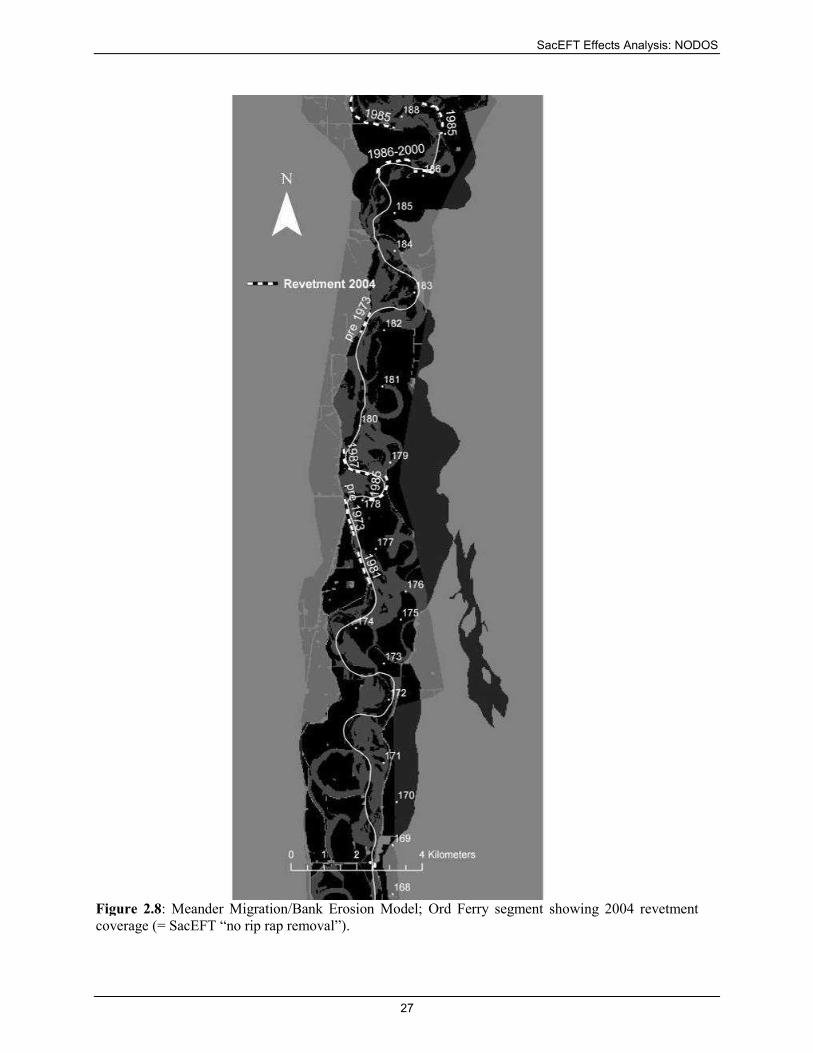
Figure 3.1: Flow exceedance plots at Keswick, RM301 (Oct-1 to Sep-30) for NODOS alternatives relative
to historical flows. .................................................................................................................................. 28
Figure 3.2: Flow exceedance plots at Bend Bridge near Red Bluff, RM260 (Oct-1 to Sep-30) for NODOS
alternatives relative to historical flows. .................................................................................................. 29
Figure 3.3: Flow exceedance plots near Hamilton City, RM199 (Oct-1 to Sep-30) for NODOS alternatives
relative to historical flows. ..................................................................................................................... 29
Figure 3.4: Flow exceedance plots near Colusa, RM143 (Oct-1 to Sep-30) for NODOS alternatives relative
to historical flows. .................................................................................................................................. 30
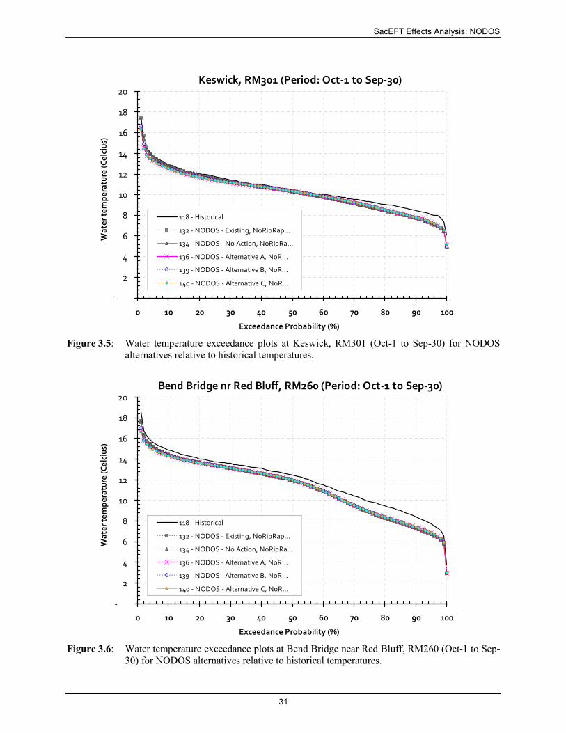
Figure 3.5: Water temperature exceedance plots at Keswick, RM301 (Oct-1 to Sep-30) for NODOS
alternatives relative to historical temperatures. ...................................................................................... 31
Figure 3.6: Water temperature exceedance plots at Bend Bridge near Red Bluff, RM260 (Oct-1 to Sep-30)
for NODOS alternatives relative to historical temperatures. .................................................................. 31
Figure 3.7: Water temperature exceedance plots near Hamilton City, RM199 (Oct-1 to Sep-30) for NODOS
Figure 3.9: Multi-year roll-up results for green sturgeon thermal egg mortality (GS1). .......................................... 40
Figure 3.10: The percentage of years in each NODOS simulation having favorable (green) conditions for
green sturgeon thermal egg mortality (GS1). Bars labeled with “Change” refer to the % change
between the simulated alternative and the reference condition (either Existing conditions or the
No Action Alternative (NAA)). ............................................................................................................. 40
Figure 3.11: Number of days in each simulation where water temperatures near Hamilton City (RM199) are
greater than 20°C. Bars labeled with “Change” refer to the change in number of days greater than 20°C between the simulated alternative and the reference condition (either Existing conditions or the No Action Alternative (NAA)). .................................................................................. 41
Figure 3.12: Target/favorable water temperature profiles (green) for minimizing green sturgeon thermal egg
mortality (GS1) at two index locations (RM260 and RM199). Water temperature profiles in
green refer to years where SacEFT’s annual performance measure rating was assessed as
good/favorable. The heavy black line provides the median of the all year favorable water
temperature profiles. Lines in red show example years rated as poor by SacEFT (i.e., highest
category of egg mortality). Horizontal lines at 17°C and 20°C are important thresholds that affect green sturgeon egg development (GS1). [Note: this figure is designed for color printing]. ........ 42
Figure 3.13: SacEFT detailed output report for a specific water year (1977) showing daily results for green
sturgeon thermal egg mortality (GS1) at a specific index location (Hamilton City). ............................. 43
Figure 3.14: The percentage of years in each NODOS simulation having favorable (green) conditions for
Steelhead spawning WUA (ST1). Bars labeled with “Change” refer to the % change between
the simulated alternative and the reference condition (either Existing conditions or the No
Action Alternative (NAA)). ................................................................................................................... 44
Figure 3.15: The percentage of years in each NODOS simulation having favorable (green) conditions for
Steelhead redd dewatering (ST6). Bars labeled with “Change” refer to the % change between
the simulated alternative and the reference condition (either Existing conditions or the No
Action Alternative (NAA)). ................................................................................................................... 44
Figure 3.16: The percentage of years in each NODOS simulation having favorable (green) conditions for
Steelhead redd scour (ST5). Bars labeled with “Change” refer to the % change between the
simulated alternative and the reference condition (either Existing conditions or the No Action
Alternative (NAA)). ............................................................................................................................... 45
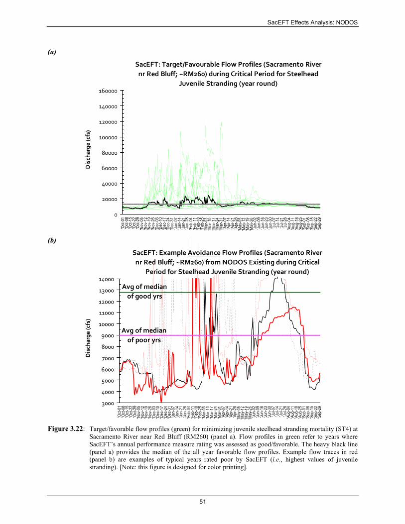
Figure 3.17: The percentage of years in each NODOS simulation having favorable (green) conditions for
Steelhead juvenile stranding (ST4). Bars labeled with “Change” refer to the % change between
the simulated alternative and the reference condition (either Existing conditions or the No
Action Alternative (NAA)). ................................................................................................................... 45
Figure 3.18: The percentage of years in each NODOS simulation having favorable (green) conditions for
Steelhead rearing WUA (ST2). Bars labeled with “Change” refer to the % change between the
simulated alternative and the reference condition (either Existing conditions or the No Action
Alternative (NAA)). ............................................................................................................................... 46
Figure 3.19: Target/favorable flow profiles (green) for steelhead spawning WUA (ST1) at Sacramento River
near Red Bluff (RM260). Flow profiles in green refer to years where SacEFT’s annual
performance measure rating was assessed as good/favorable. The heavy black line provides the
median of the all year favorable flow profiles. The grey horizontal line (panel a) is the average
of the median target flow. Flow traces in red (panel b) are examples of typical years rated poor
by SacEFT (i.e., least cumulative spawning habitat potential). [Note: this figure is designed for
color printing]. ....................................................................................................................................... 47
Figure 3.20: Example target/favorable flow profiles (green) for steelhead redd dewatering (ST6) at
Sacramento River near Red Bluff (RM260) (panel a). Flow profiles in green refer to years
where SacEFT’s annual performance measure rating was assessed as good/favorable. Example
flow traces in red (panel b) are examples of typical years rated poor by SacEFT (i.e., highest
values of redd dewatering). .................................................................................................................... 48
SacEFT Effects Analysis: NODOS
vi
Figure 3.21: Target/favorable flow profiles (green) for minimizing steelhead egg scour mortality (ST5) at
Sacramento River near Red Bluff (RM260) (panel a). Flow profiles in green refer to years
where SacEFT’s annual performance measure rating was assessed as good/favorable. The heavy
black line (panel a) provides the median of the all year favorable flow profiles. Example flow
traces in red (panel b) are examples of typical years rated poor by SacEFT (i.e., highest values
of redd scour). Horizontal lines at 55,000 cfs and 75,000 cfs are important thresholds that affect
Operations Priorities (Primary Planning Objectives) Long Term (all years) EESA4
Power5 EESA4 Power5
EESA4 Power5
Driest Periods (drought years) M&I M&I M&I Average to Wet Periods (non-drought years)
Water Quality Level 4 Refuge
Agricultural
Water Quality Level 4 Refuge
Agricultural
Water Quality Level 4 Refuge
Agricultural Notes: 1. Diversions through the TC Canal, GCID Canal, and Delevan Pipeline are allowed in any month of the year. 2. New Delevan Pipeline can be operated June through March (April and May are reserved for maintenance). 3. A pump station, intake, and fish screens are not included for the Delevan Pipeline for Alternative B. For Alternative B, the
Delevan Pipeline will be operated for releases only from Sites Reservoir to the Sacramento River year round. 4. Ecosystem Enhancement Storage Account (EESA) related operations are a function of specific conditions, and operating
criteria that are defined uniquely for each action. 5. Includes dedicated pump/generation facilities with an additional dedicated after-bay/fore-bay (enlarged Funks Reservoir) used
for managing conveyance of water between Sites Reservoir and river diversion locations. Key: cfs = cubic feet per second CVP = Central Valley Project EESA = ecosystem enhancement storage account MAF = million acre-feet M&I = municipal and industrial SWP = State Water Project TAF = thousand acre-feet
1.2.1 Ecosystem Enhancement Actions
The proposed NODOS alternatives include the following Ecosystem Enhancement Actions (EEAs):
Action 1. Improve the reliability of coldwater pool storage in Shasta Lake to increase the US Bureau of
Reclamation’s operational flexibility to provide suitable water temperatures in the Sacramento River (see
Action 2 below). This action would operationally translate into the increase of Shasta Lake May storage
SacEFT Effects Analysis: NODOS
7
levels, and increased coldwater pool in storage, with particular emphasis on Below Normal, Dry and
Critical water year types.
Action 2. Provide releases from Shasta Dam of appropriate water temperatures, and subsequently from
Keswick Dam, to maintain mean daily water temperatures year-round at levels suitable for all species and
life-stages of anadromous salmonids in the Sacramento River between Keswick Dam and Red Bluff
Diversion Dam, with particular emphasis on the months of highest potential water temperature-related
impacts (i.e., July through November) during Below Normal, Dry and Critical water year types.
Action 3. Increase the availability of coldwater pool storage in Folsom Reservoir, by increasing May
storage and coldwater pool storage, to allow the U.S. Bureau of Reclamation additional operational
flexibility to provide suitable water temperatures in the lower American River. This action would utilize
additional coldwater pool storage by providing releases from Folsom Dam (and subsequently from
Nimbus Dam) to maintain mean daily water temperatures at levels suitable for juvenile steelhead over-
summer rearing and fall-run Chinook salmon spawning in the lower American River from May through
November during all water year types (not explicitly modeled in CALSIM II).
Action 4. Provide supplemental Delta outflow during summer and fall months (i.e., May through
December) to improve X2 (if possible, west of Collinsville, 81 km) and increase estuarine habitat, reduce
entrainment, and improve food availability for anadromous fishes and other estuarine-dependent species
(e.g., delta smelt, longfin smelt, Sacramento splittail, starry flounder, and the shrimp Crangon
franciscorum).
Action 5. Improve the reliability of coldwater pool storage in Lake Oroville to improve water temperature
suitability for juvenile steelhead and spring-run Chinook salmon over-summer rearing and fall-run
Chinook salmon spawning in the lower Feather River from May through November during all water year
types. Provide releases from Oroville Dam to maintain mean daily water temperatures at levels suitable
for juvenile steelhead and spring-run Chinook salmon over-summer rearing, and fall-run Chinook salmon
spawning in the lower Feather River. Stabilize flows in the lower Feather River to minimize redd
dewatering, juvenile stranding and isolation of anadromous salmonids.
Action 6. Stabilize flows in the Sacramento River between Keswick Dam and the Red Bluff Diversion
Dam to minimize dewatering of fall-run Chinook salmon redds (for the spawning and embryo incubation
life-stage periods extending from October through March), particularly during fall months.
Action 7. Provide increased flows from spring through fall in the lower Sacramento River by reducing
diversions at Red Bluff Diversion Dam (into the Tehama-Colusa Canal) and at Hamilton City (into the
Glenn-Colusa Irrigation District Canal), and by providing supplemental flows (at Delevan). This action
will provide multiple benefits to riverine and estuarine habitats, and to anadromous fishes and estuarine-
dependent species (e.g., delta smelt, splittail, longfin smelt, Sacramento splittail, starry flounder, and the
shrimp Crangon franciscorum) by reducing entrainment, providing or augmenting transport flows,
increasing habitat availability, increasing productivity, and improving nutrient transport and food
availability.
SacEFT Effects Analysis: NODOS
8
2. Methodology and Assumptions
Details on SacEFT performance measure algorithms and their science foundation are beyond the scope of
this document. Please refer to the SacEFT Record of Design for a complete description of model
performance measures and assumptions (ESSA 2011).
2.1 SacEFT’s Focal Species and Performance Measures
Chinook Salmon
(Oncorhynchus tshawytscha)
Steelhead
(Oncorhynchus mykiss)
Green Sturgeon
(Acipenser medirostris)
Bank Swallow
(Riparia riparia)Western Pond Turtle
(Clemmys marmorata)
Fremont Cottonwood
(Populus fremontii)
SacEFT focal species
SacEFT’s focal species and performance measures – discussed in detail in ESSA (2011) – are listed in
Table 2-A. The sections that follow below provide a brief summary of SacEFT’s focal species and
performance measures.
SacEFT Effects Analysis: NODOS
9
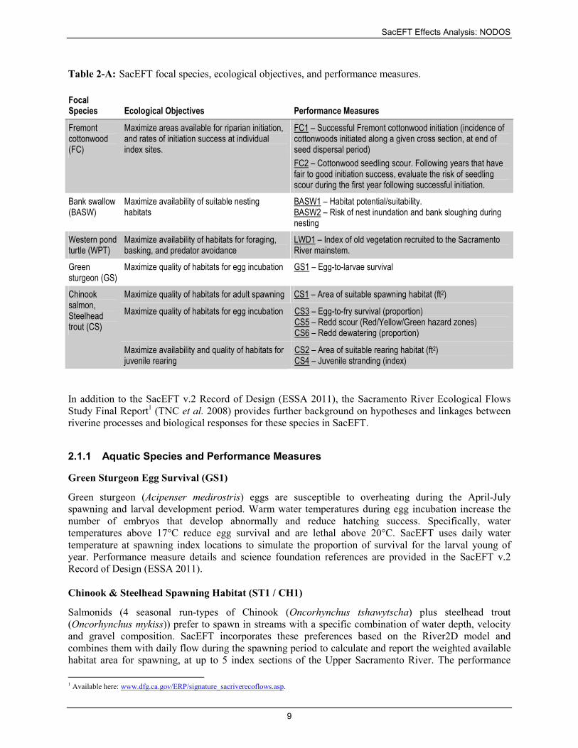
Table 2-A: SacEFT focal species, ecological objectives, and performance measures.
Focal Species Ecological Objectives Performance Measures
Fremont cottonwood (FC)
Maximize areas available for riparian initiation, and rates of initiation success at individual index sites.
FC1 – Successful Fremont cottonwood initiation (incidence of cottonwoods initiated along a given cross section, at end of seed dispersal period)
FC2 – Cottonwood seedling scour. Following years that have fair to good initiation success, evaluate the risk of seedling scour during the first year following successful initiation.
Bank swallow (BASW)
Maximize availability of suitable nesting habitats
BASW1 – Habitat potential/suitability. BASW2 – Risk of nest inundation and bank sloughing during nesting
Western pond turtle (WPT)
Maximize availability of habitats for foraging, basking, and predator avoidance
LWD1 – Index of old vegetation recruited to the Sacramento River mainstem.
Green sturgeon (GS)
Maximize quality of habitats for egg incubation GS1 – Egg-to-larvae survival
Chinook salmon, Steelhead trout (CS)
Maximize quality of habitats for adult spawning CS1 – Area of suitable spawning habitat (ft2)
Table 2-D: Annotations for Table 2-B and Table 2-C. 1 The common time span of Historic discharge (Q) data is 1-Oct-1938 to 30-Sep-2004. The common time span of
Historic temperature (T) data is 1-Jan-1970 to 31-Dec-2001.
2 The common time span of the NODOS scenario analyses performed in April 2011 include discharge (Q) and
temperature (T) data between 1-Oct-1921 to 30-Sep-2003.
3 TUGS simulations (Cui 2007) shown in red actually comprise 5 distinct reaches between RM 301 and RM 289. TUGS
results are not available downstream from Cow Creek but are necessary for linkage to Chinook and Steelhead spawning
Weighted Usable Area (WUA) (CS1). TUGS relationships for these downstream segments (pink) are mapped from the
nearest upstream location, as described in ESSA (2011).
4 Chinook and Steelhead spawning WUA relationships shown in pale blue are mapped from the closest downstream
segment, as described in ESSA (2011). Spring Chinook habitat preferences are assumed to follow those of fall Chinook.
Chinook rearing WUA relationships shown in pale blue are mapped from the closest upstream section, as describe in
ESSA (2011).
5 The BDCP analysis performed in June of 2010 included a subset of PMs: Chinook, Steelhead and green sturgeon in the
region from Keswick to Hamilton City only.
The Meander Migration model is based on empirical river centerlines measured in 2004. For the meander
(and bank erosion) simulations, WY1922 NODOS flows were applied starting with the 2004 river
centerlines and this centerline run forwards for 82 years. Note that the first year of the simulation results
(WY1922) was not included in SacEFT due to numerical instability of the meander migration results prior
to burn-in. As a result, SacEFT results for NODOS are displayed beginning in WY1923. For the historical
case, results are run forward for 65 years beginning in WY1939.
SacEFT Effects Analysis: NODOS
21 The Nature Conservancy
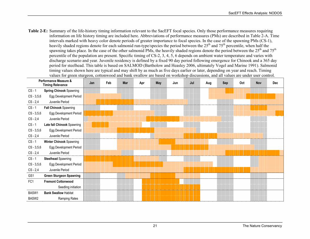
Table 2-E: Summary of the life-history timing information relevant to the SacEFT focal species. Only those performance measures requiring
information on life history timing are included here. Abbreviations of performance measures (PMs) are described in Table 2-A. Time
intervals marked with heavy color denote periods of greater importance to focal species. In the case of the spawning PMs (CS-1),
heavily shaded regions denote for each salmonid run-type/species the period between the 25th and 75
th percentile, when half the
spawning takes place. In the case of the other salmonid PMs, the heavily shaded regions denote the period between the 25th and 75
th
percentile of the population are present. Specific timing of CS-2, 3, 4, 5, 6 depends on ambient water temperature and varies with
discharge scenario and year. Juvenile residency is defined by a fixed 90 day period following emergence for Chinook and a 365 day
period for steelhead. This table is based on SALMOD (Bartholow and Heasley 2006, ultimately Vogel and Marine 1991). Salmonid
timing values shown here are typical and may shift by as much as five days earlier or later, depending on year and reach. Timing
values for green sturgeon, cottonwood and bank swallow are based on workshop discussions, and all values are under user control.
Performance Measure & Timing Relevance
Jan Feb Mar Apr May Jun Jul Aug Sep Oct Nov Dec
CS - 1 Spring Chinook Spawning
CS - 3,5,6 Egg Development Period
CS - 2,4 Juvenile Period
CS - 1 Fall Chinook Spawning
CS - 3,5,6 Egg Development Period
CS - 2,4 Juvenile Period
CS - 1 Late fall Chinook Spawning
CS - 3,5,6 Egg Development Period
CS - 2,4 Juvenile Period
CS - 1 Winter Chinook Spawning
CS - 3,5,6 Egg Development Period
CS - 2,4 Juvenile Period
CS - 1 Steelhead Spawning
CS - 3,5,6 Egg Development Period
CS - 2,4 Juvenile Period
GS1 Green Sturgeon Spawning
FC1 Fremont Cottonwood
Seedling initiation
BASW1 Bank Swallow Habitat
BASW2 Ramping Rates
SacEFT Effects Analysis: NODOS
22 The Nature Conservancy
2.4 Special Conditions and Limitations
Although the NODOS Investigation alternatives provide daily flow and temperature data for the
WY1922–2003 period, most of the salmonid results from SacEFT in this analysis are unavailable prior to
WY1939. This gap is a consequence of the required linkage between the calculation of spawning habitat
and streambed gravel grain size-distribution. SacEFT requires annual estimates of the gravel grain size-
distribution at each of 5 river segments in order to calculate the weighted useable area available for
spawning (ST1/CH1). This habitat estimate is then used as one of the inputs to calculate subsequent
performance measures for egg maturation, survival, and juvenile rearing. In the absence of gravel data, no
calculations are possible for these linked components. For previous model analyses using SacEFT,
colleagues at Stillwater Sciences calibrated and ran The Unified Gravel & Sand (TUGS) model (Cui
2007) over the WY1939-2004 period and provided this information for input to a number of SacEFT
scenarios that all used this common time-frame. TUGS simulates changes in grain size of the river by
accounting for how its sediment flux interacts with sediment in both the surface and subsurface of the
channel bed. Time constraints for the current investigation prevented this level of engagement with
Stillwater Sciences, and we were therefore required to re-use the “default historical gravel” scenario data
(Stillwater Sciences 2007). This data was applied starting in WY1939 in the NODOS alternatives to
ensure that the time series lengths matched. This is a known limitation of the results for the ST1/CH1
performance measures in this analysis, but does not have a significant bearing on the other 5 ST/CH
performance measures.
2.5 Focal Comparisons
DWR and the US Bureau of Reclamation NODOS Investigation team have defined the storage and
conveyance alternatives for evaluation in the North-of-the-Delta Offstream Storage Draft Environmental
Impact Report and Statement (DEIR/EIS). These alternatives are described in section 1.2. Results of the
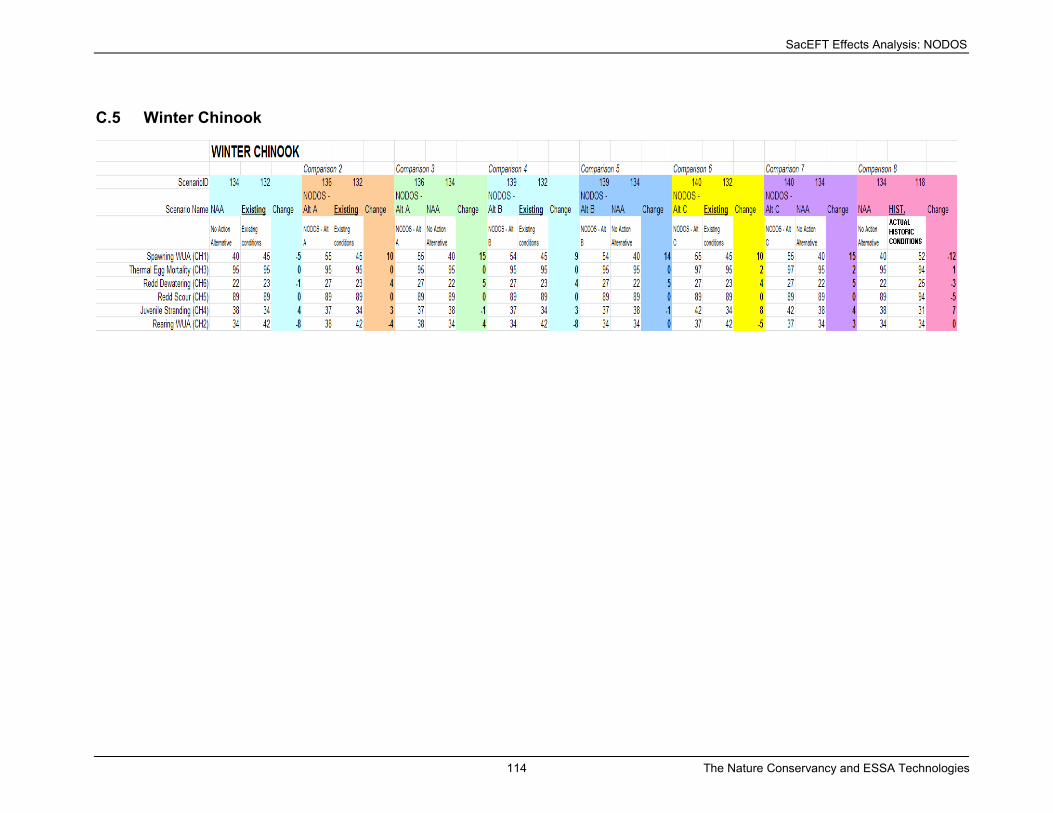
SacEFT ecological effects analysis are organized by species for the following eight comparisons:
Comparison NODOS Alternative (SacEFT ID) Compared to (SacEFT ID)
1 No Action Alternative (134) Existing Conditions (132)
2 A (136) Existing Conditions (132)
3 A (136) No Action Alternative (134)
4 B (139) Existing Conditions (132)
5 B (139) No Action Alternative (134)
6 C (140) Existing Conditions (132)
7 C (140) No Action Alternative (134)
8* No Action Alternative (134) Historic conditions (118) *This is not a recognized EIS/EIR comparison. CEQA/NEPA which emphasize isolating project alternative effects as compared to a No Action reference or Existing condition comparison.
Comparison 8 is not used in our report to assess NODOS effects. Instead, it provides an essential
reference case illustrating how SacEFT’s various performance measures have performed under historic
flows and water temperatures from WY1938–2003. Relative to future hydrosystem operations, these
flows represent more natural patterns of variation in flow and water temperature that have occurred
historically.
2.5.1 SacEFT Gravel Augmentation and Bank Protection Alternatives
In addition to analyzing the NODOS alternative flow and water temperature regimes, SacEFT enables
comparisons of gravel augmentation and rock removal restoration actions. The NODOS alternatives,
including the No Action Alternative, do not include gravel augmentation or bank protection
SacEFT Effects Analysis: NODOS
23 The Nature Conservancy
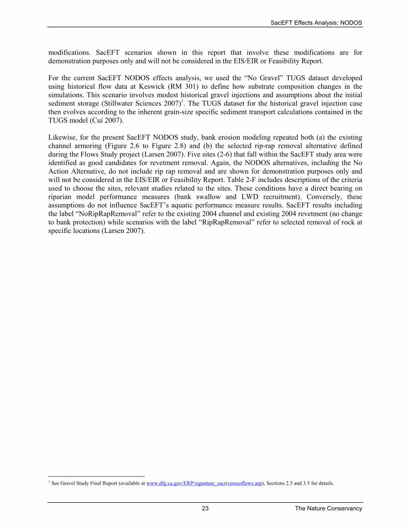
modifications. SacEFT scenarios shown in this report that involve these modifications are for
demonstration purposes only and will not be considered in the EIS/EIR or Feasibility Report.
For the current SacEFT NODOS effects analysis, we used the “No Gravel” TUGS dataset developed
using historical flow data at Keswick (RM 301) to define how substrate composition changes in the
simulations. This scenario involves modest historical gravel injections and assumptions about the initial
sediment storage (Stillwater Sciences 2007)1. The TUGS dataset for the historical gravel injection case
then evolves according to the inherent grain-size specific sediment transport calculations contained in the
TUGS model (Cui 2007).
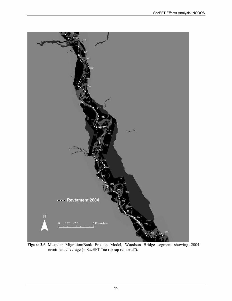
Likewise, for the present SacEFT NODOS study, bank erosion modeling repeated both (a) the existing
channel armoring (Figure 2.6 to Figure 2.8) and (b) the selected rip-rap removal alternative defined
during the Flows Study project (Larsen 2007). Five sites (2-6) that fall within the SacEFT study area were
identified as good candidates for revetment removal. Again, the NODOS alternatives, including the No
Action Alternative, do not include rip rap removal and are shown for demonstration purposes only and
will not be considered in the EIS/EIR or Feasibility Report. Table 2-F includes descriptions of the criteria
used to choose the sites, relevant studies related to the sites. These conditions have a direct bearing on
riparian model performance measures (bank swallow and LWD recruitment). Conversely, these
assumptions do not influence SacEFT’s aquatic performance measure results. SacEFT results including
the label “NoRipRapRemoval” refer to the existing 2004 channel and existing 2004 revetment (no change
to bank protection) while scenarios with the label “RipRapRemoval” refer to selected removal of rock at
specific locations (Larsen 2007).
1 See Gravel Study Final Report (available at www.dfg.ca.gov/ERP/signature_sacriverecoflows.asp), Sections 2.5 and 3.5 for details.
Table 2-F: Potential revetment removal sites on the middle Sacramento River. Sites 2-6 define the “rip rap removal” scenario in SacEFT. For
details see Larsen (2007).
Site No. Site Name River Mile Length
(meters +/-)
Adjoining Landowner Revetment Material Description / Notes Relevant
Meander
Analysis
Data Number
on Google
Earth File
1 La Barranca 240.5R 550 USFWS - La Barranca Unit,
Sacramento River NWR
Medium rock Lower 1/3 of a larger revetment area is adjacent to La Barranca Unit,
removal would also take pressure of rock at 240L
A Reach 2 - 981
2 Kopta Slough 220-222R 1775 State Controller's Trust (TNC is
lessee)
Medium rock Area is being converted to habitat, removal would help redirect erosion
from State Recreation Area and County bridge, substantial planning
work has occurred
A, B Reach 2 - 5819
3 Rio Vista 216-217L 1425 USFWS - Rio Vista Unit, Sacramento
River NWR
Large rock, privately
installed
Rock was installed to protect agriculture, the area is now converted to
habitat
A Reach 2 - 1069,
1183, 4674
4 Brayton 197-198R 600 CDPR, Bidwell-Sac River St Park,
Brayton property
Large rubble, privately
installed
Rock was installed to protect agriculture, the area is planned to be
converted to habitat, consider effect on the road to the east but geologic
control should limit meander
A, C Reach 2 - 2007
5 Phelan island 191-192R 1410 USFWS, Phelan Island Unit and Sac &
San Joaquin Drainage Dist.
Medium rock, USACE
installed in 1988
Area has been converted to habitat, consider possible Murphy's Slough
cutoff / flood relief structure concerns
A, C, E Reach 3 - 4626
6 Llano Seco
Riparian
Sanctuary
179R 1300 USFWS, Phelan Island Unit and Sac &
San Joaquin Drainage District and small
area of private property
Medium rock, USACE
installed in 1985 & 87
Rock removal potential identified as part of Lano Seco Riparian
Sanctuary planning project as part of a solution to fish screen concerns
at Princeton, Codora/ Provident pumping plant at RM 178R
D Reach 3 - 2805,
1422
Initial screening and review included staff from DWR Northern District, Sacramento River Conservation Area Forum and The Nature Conservancy
Criteria for Revetment Removal Identification
1. Revetment is adjacent to public or conservation ownership land
2. Revetment is not protecting important public infrastructure
3. Revetment removal does not create an obvious flood hazard
4. Revetment is currently limiting meander on lands in the historic meander belt
5. Revetment removal could result in ecosystem benefit: land reworking/creation of riparian habitat, creation of new bank swallow habitat, recruitment of spawning gravel, new shaded riverine aquatic habitat, etc.
5. Revetment removal could help direct meander to protect public infrastructure (if applicable)
Relevant Meander Analysis References
A. Department of Water Resources, Northern District, 1991, 25 and 50-year erosion projections for the Sacramento River.
B. Larsen, Eric, 2002. Modeling Channel Management Impacts on River Migration: A Case Study of Woodson Bridge state Recreation Area, Sacramento River, USA. University of California, Davis, Davis, California.
C. Larsen, Eric, 2002. The Control and Evolution of Channel Morphology of the Sacramento River: A Case Study of River Miles 201-185. University of California, Davis, Davis, California.
D. Larsen, Eric, 2004. Meander Bend Migration near River Mile 178 of the Sacramento River. University of California, Davis, Davis, California.
E. Larsen, Eric, 2005. Future Meander Bend Migration and Floodplain Development Patterns near River Miles 200 to 191 of the Sacramento River. University of California, Davis, Davis, California.
POTENTIAL REVETMENT REMOVAL SITES ON THE MIDDLE SACRAMENTO RIVER
Bank Swallows Habitat potential/suitability (BASW1)** ni (+1)
Peak flow during nesting period (BASW2) + (+4)
Western Pond Turtles Large Woody Debris Recruitment (LWD)** - - (-29)
Green Sturgeon Egg temperature preferences (GS1) n/a
Steelhead Spawning WUA (ST1) ++ (+14)
Thermal egg mortality (ST3) ni (+/-0)
Redd Dewatering (ST6) + (+9)
Redd Scour (ST5) - - (-16)
Juvenile Stranding (ST4) - - (-24)
Rearing WUA (ST2) ++ (+13)
Fall Chinook Spawning WUA (CH1) - - (-15)
Thermal egg mortality (CH3) + (+8)
Redd Dewatering (CH6) + (+4)
Redd Scour (CH5) - (-5)
Juvenile Stranding (CH4) - - (-25)
Rearing WUA (CH2) ni (+1)
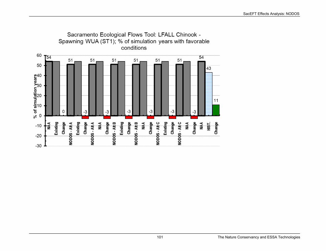
Late Fall Chinook Spawning WUA (CH1) ++ (+11)
Thermal egg mortality (CH3) ni (+/-0)
Redd Dewatering (CH6) + (+6)
Redd Scour (CH5) - - (-13)
Juvenile Stranding (CH4) - - (-11)
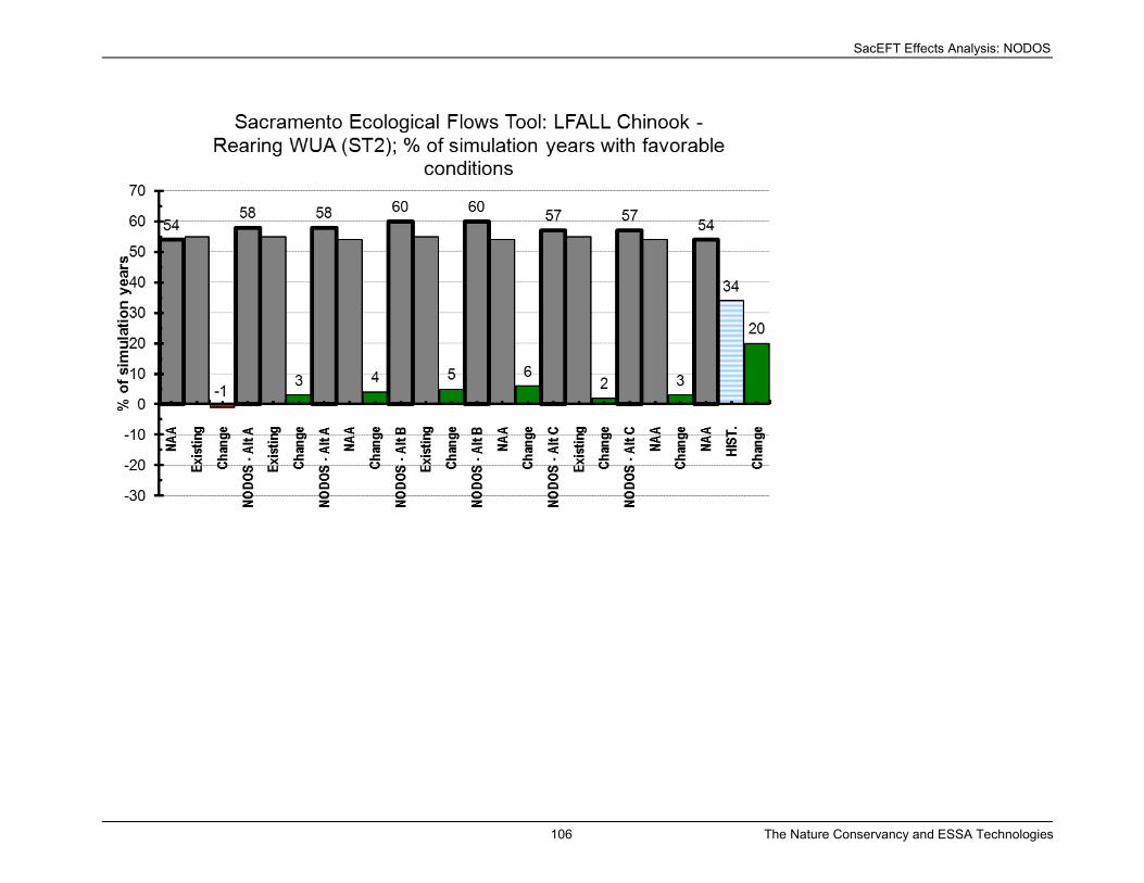
Rearing WUA (CH2) ++ (+20)
Spring Chinook Spawning WUA (CH1) ni (-2)
Thermal egg mortality (CH3) + (+8)
Redd Dewatering (CH6) ++ (+35)
Redd Scour (CH5) ni (+/-0)
Juvenile Stranding (CH4) - - (-29)
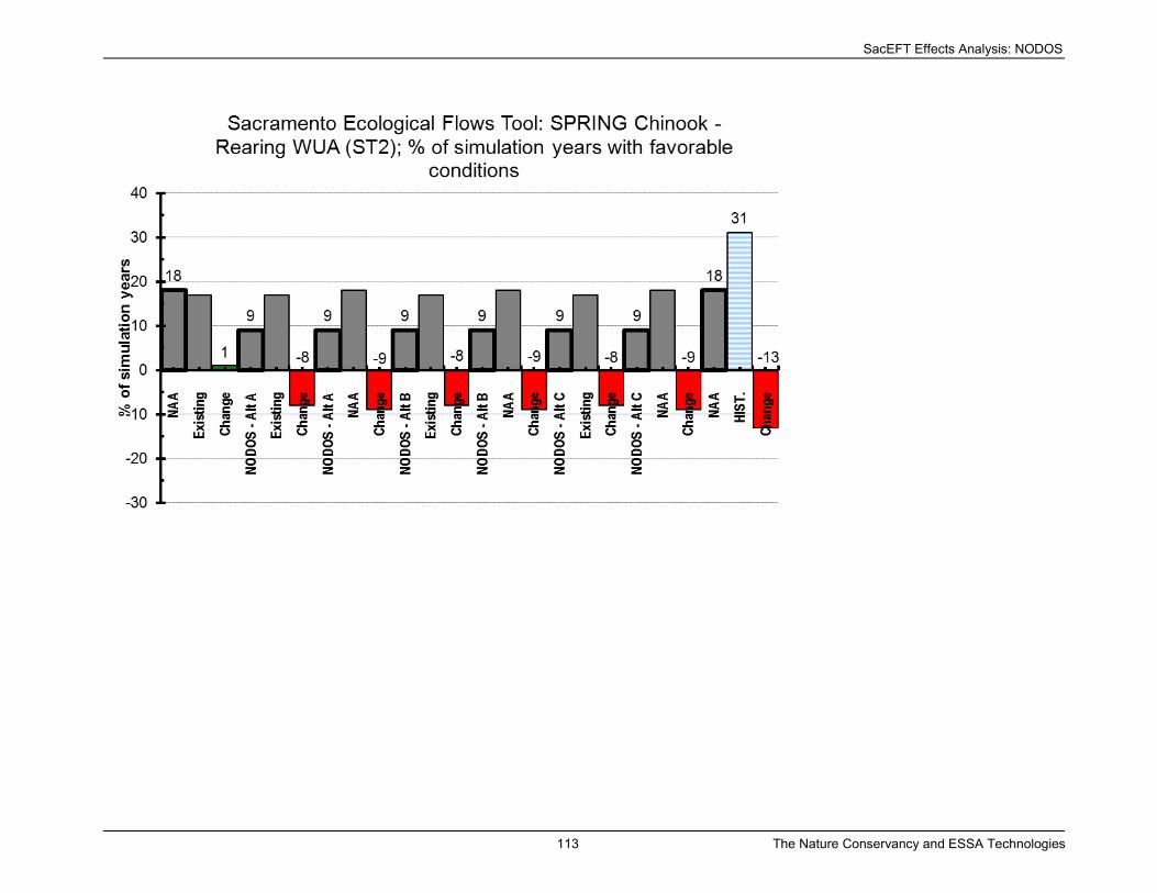
Rearing WUA (CH2) - - (-13)
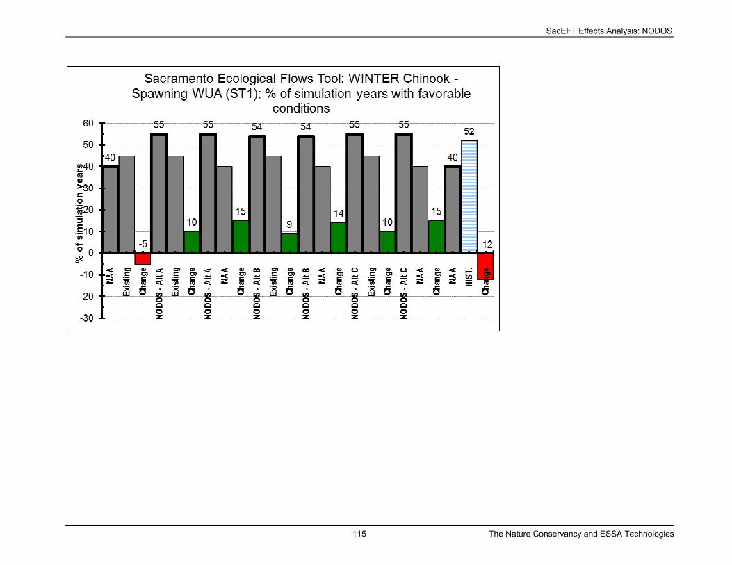
Winter Chinook Spawning WUA (CH1) - - (-12)
Thermal egg mortality (CH3) ni (+1)
Redd Dewatering (CH6) ni (-3)
Redd Scour (CH5) - (-5)
SacEFT Effects Analysis: NODOS
39
Focal species Performance measure
NAA vs.
Historic Conditions (Comparison 8)
Juvenile Stranding (CH4) + (+7)
Rearing WUA (CH2) ni (+/-0)
Legend ++
+
ni
-
--
strong beneficial impact owing to project alternative
small beneficial impact owing to project alternative
negligible detected impact owing to project alternative
small negative impact owing to project alternative
strong negative impact owing to project alternative
The purpose of the environmental and feasibility documents is to describe the difference between No
Action / Existing Conditions and the Action Alternatives which all reflect 2030 conditions, constraints
and operations. Typically, none of the NODOS Investigation alternative modelling results are compared
against the historical calibration due to the focus of CEQA/NEPA which emphasizes isolating project
alternative effects as compared to a no action reference or existing condition comparison.
Comparison #8 (see Section 2.5; The NAA, relative to Actual Historic Conditions) is not used in our
report to assess NODOS effects. Instead, it provides an essential reference case illustrating how SacEFT’s
various performance measures have performed under historic flows and water temperatures from 1938 –
2003 relative to the future 2030 conditions, constraints and hydrosystem operations in the NAA. Historic
flows represent less constrained, more natural patterns of variation in flow and water temperature that
have occurred in the past. Comparisons that include historical data reveal different information in a
different context that does not address a specific project effect relative to the no action alternative or
existing condition reference case. These comparisons identify the ecological effects of the future system
operations and constraints relative to historic conditions. In fully considering ecological flow needs, the
magnitude of departure from these historic conditions may reveal important information on how future
constraints, climate and/or hydrosystem operational modifications are influencing preferred ecological
flow targets. Historic flows represent less constrained, more natural patterns of variation in flow and
water temperature that have occurred in the past.
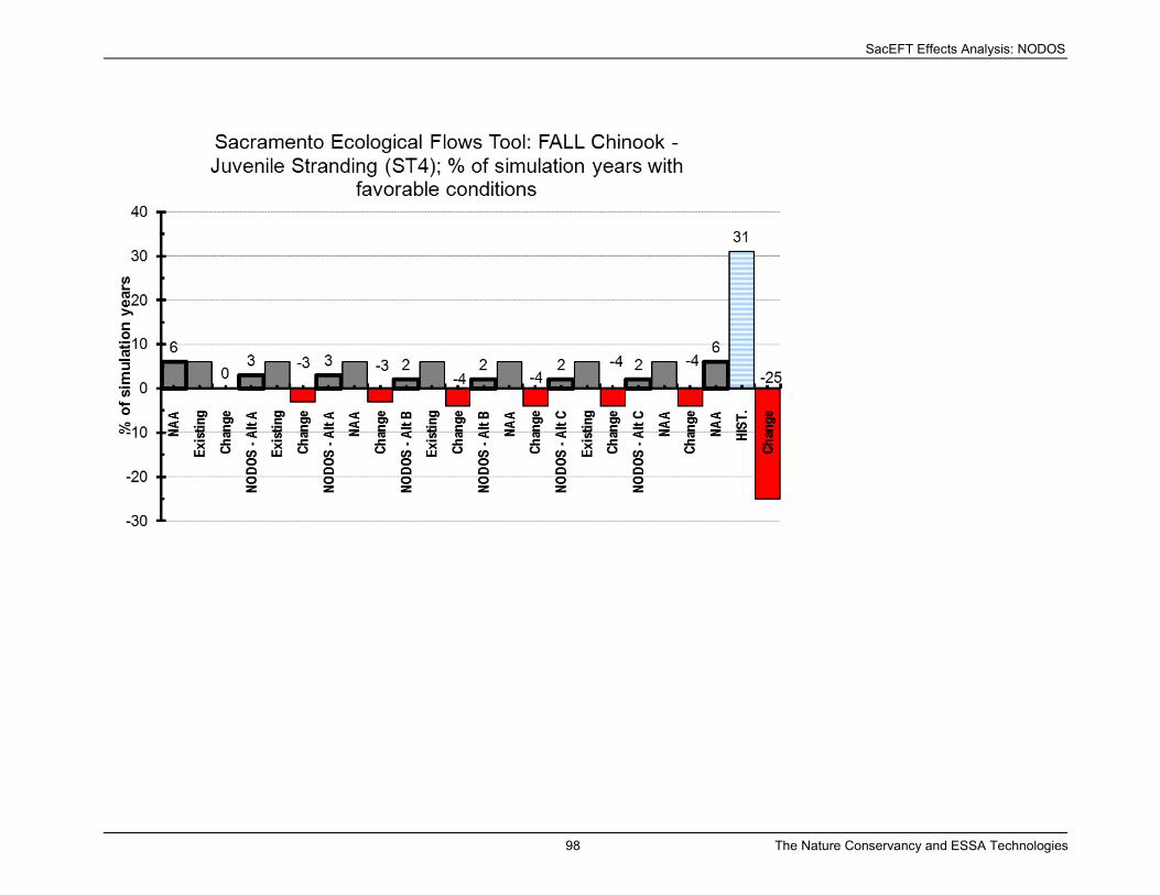
Table 3-D shows that relative to historic flows and water temperatures, conditions associated with the
NAA (comparison 8) generate a strong negative effect on Fremont Cottonwood initiation success (FC1),
Large Woody Debris recruitment (LWD) and Steelhead/fall Chinook/late fall Chinook/spring Chinook
juvenile stranding risk (ST4/CH4). For case #8, fall Chinook spawning WUA (CH1) performance
declined, as it did for winter-run Chinook. Likewise, redd scour risk is increased for Steelhead (ST5) and
late fall Chinook (CH5). Rearing WUA (CH2) habitat conditions were also lower in the case of spring run
Chinook
The following performance measures showed a strong positive effect owing to the NAA relative to actual
historic conditions: Steelhead and late fall Chinook spawning WUA (ST1 and CH1). Also improved were
rearing WUA for late fall Chinook (CH2). Notably, as with NODOS alternatives A, B and C, spring
Chinook redd dewatering risk (CH6) was markedly reduced by conditions present in the NAA vs. actual
historic.
SacEFT Effects Analysis: NODOS
40
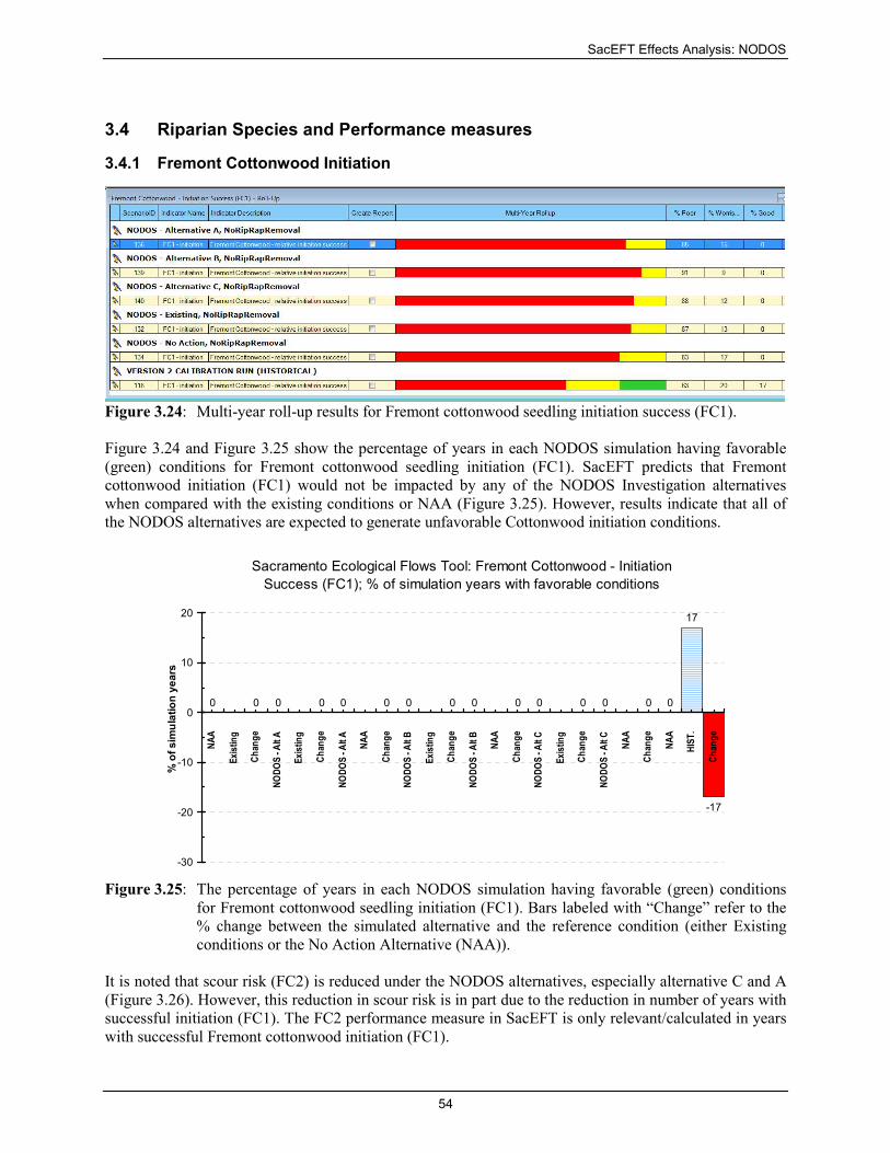
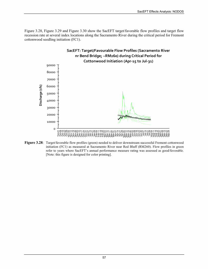
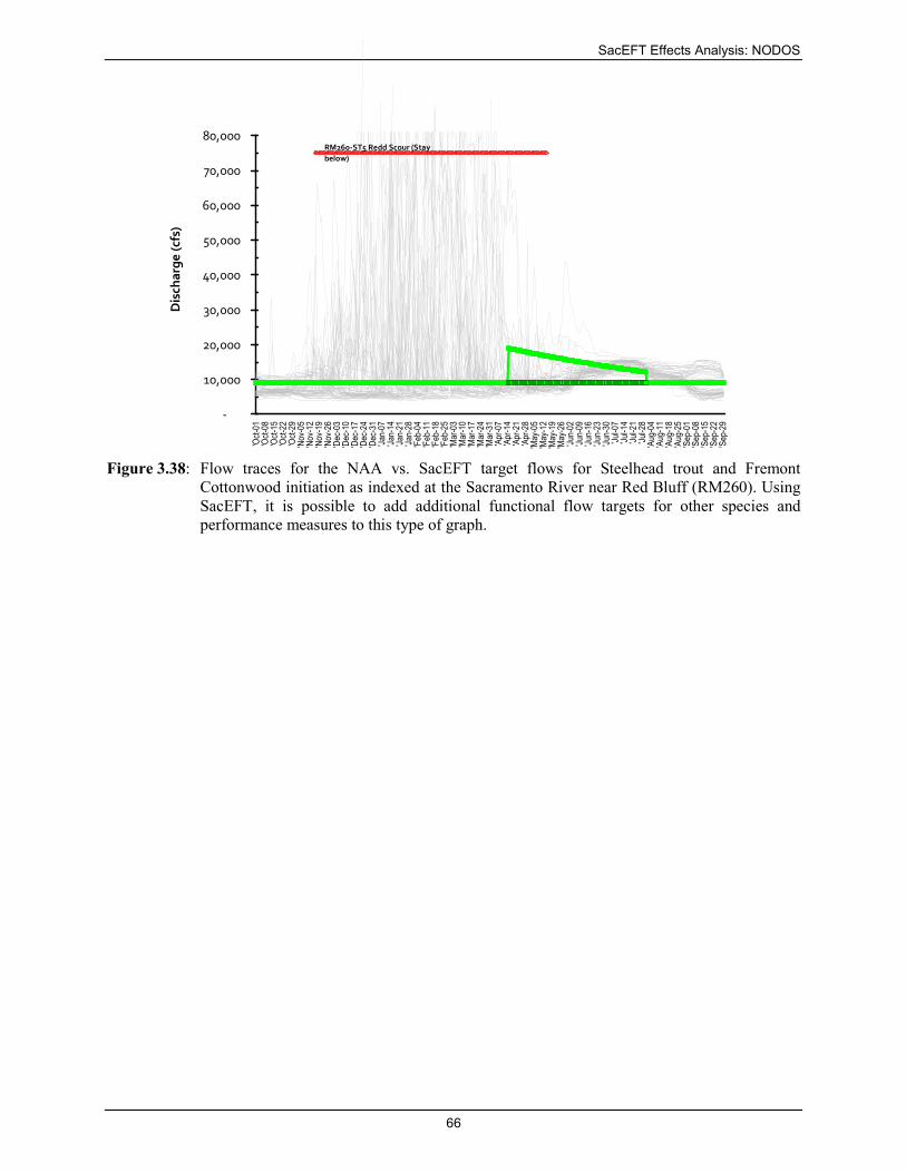
3.3 Aquatic Species and Performance Measures
3.3.1 Green Sturgeon
Figure 3.9: Multi-year roll-up results for green sturgeon thermal egg mortality (GS1).
Figure 3.9 and Figure 3.10 show the percentage of years in each NODOS simulation having favorable
(green) conditions for green sturgeon thermal egg mortality (GS1). SacEFT predicts that green sturgeon
eggs (GS1) would receive benefits (+5% to +8% of years with better conditions) from all three of the
NODOS Investigation alternatives in terms of reduction of thermal egg mortality (GS1) (Figure 3.10).
Figure 3.11 shows the number of days in each simulation that water temperatures are above the 20°C lethal threshold for green sturgeon egg development. Consistent with SacEFT preferred condition roll-up
results, the NODOS Investigation alternatives all reduce the number of days green sturgeon eggs are
exposed to lethal water temperatures.
Sacramento Ecological Flows Tool: Green Sturgeon - Egg
Temperature Preferences (GS1); % of simulation years with
favorable conditions
16 5
8 7 8 7
90909090888883
-30
-20
-10
0
10
20
30
40
50
60
70
80
90
100
NAA
Existing
Change
NODOS - Alt A
Existing
Change
NODOS - Alt A
NAA
Change
NODOS - Alt B
Existing
Change
NODOS - Alt B
NAA
Change
NODOS - Alt C
Existing
Change
NODOS - Alt C
NAA
Change
% o
f sim
ula
tion y
ears
Figure 3.10: The percentage of years in each NODOS simulation having favorable (green) conditions
for green sturgeon thermal egg mortality (GS1). Bars labeled with “Change” refer to the %
change between the simulated alternative and the reference condition (either Existing
conditions or the No Action Alternative (NAA)).
SacEFT Effects Analysis: NODOS
41
Sacramento Ecological Flows Tool: Green Sturgeon - Egg
Temperature Preferences (GS1); Days in Simulation Greater
Than 20C; near Hamilton City (~RM199)
-30
-20
-10
0
10
20
30
40
50
60
NAA
Existing
Change
NODOS - Alt A
Existing
Change
NODOS - Alt A
NAA
Change
NODOS - Alt B
Existing
Change
NODOS - Alt B
NAA
Change
NODOS - Alt C
Existing
Change
NODOS - Alt C
NAA
Change
Days G
reate
r Than 2
0C
Figure 3.11: Number of days in each simulation where water temperatures near Hamilton City (RM199)
are greater than 20°C. Bars labeled with “Change” refer to the change in number of days greater than 20°C between the simulated alternative and the reference condition (either Existing conditions or the No Action Alternative (NAA)).
SacEFT Target and Avoidance Flows for Green Sturgeon Egg Development
Figure 3.12 shows the SacEFT target/favorable water temperature profiles and the median target water
temperature at the Sacramento River near Red Bluff (RM260) and Hamilton City (RM199) during the
critical period for green sturgeon egg development.
SacEFT Effects Analysis: NODOS
42
SacEFT: Target/Favourable Water Temperature Profiles
(Sacramento River nr Red Bluff; ~RM260) during Green Sturgeon
Critical Period (Mar-1 to Aug-15)
17C
20C
1977
6789
1011121314151617181920212223
'Oct-01
'Oct-08
'Oct-15
'Oct-22
'Oct-29
'Nov
-05
'Nov
-12
'Nov
-19
'Nov
-26
'Dec
-03
'Dec
-10
'Dec
-17
'Dec
-24
'Dec
-31
'Jan
-07
'Jan
-14
'Jan
-21
'Jan
-28
'Feb
-04
'Feb
-11
'Feb
-18
'Feb
-25
'Mar-03
'Mar-10
'Mar-17
'Mar-24
'Mar-31
'Apr-07
'Apr-14
'Apr-21
'Apr-28
'May
-05
'May
-12
'May
-19
'May
-26
'Jun
-02
'Jun
-09
'Jun
-16
'Jun
-23
'Jun
-30
'Jul-07
'Jul-14
'Jul-21
'Jul-28
'Aug
-04
'Aug
-11
'Aug
-18
'Aug
-25
'Sep
-01
'Sep
-08
'Sep
-15
'Sep
-22
'Sep
-29
Wa
ter
Te
mp
era
ture
(C
elc
ius)
SacEFT: Target/Favourable Water Temperature Profiles
(Sacramento River nr Hamilton City; ~RM199) during Green
Sturgeon Critical Period (Mar-1 to Aug-15)
17C
20C
6789
1011121314151617181920212223
'Oct-01
'Oct-08
'Oct-15
'Oct-22
'Oct-29
'Nov
-05
'Nov
-12
'Nov
-19
'Nov
-26
'Dec
-03
'Dec
-10
'Dec
-17
'Dec
-24
'Dec
-31
'Jan
-07
'Jan
-14
'Jan
-21
'Jan
-28
'Feb
-04
'Feb
-11
'Feb
-18
'Feb
-25
'Mar-03
'Mar-10
'Mar-17
'Mar-24
'Mar-31
'Apr-07
'Apr-14
'Apr-21
'Apr-28
'May
-05
'May
-12
'May
-19
'May
-26
'Jun
-02
'Jun
-09
'Jun
-16
'Jun
-23
'Jun
-30
'Jul-07
'Jul-14
'Jul-21
'Jul-28
'Aug
-04
'Aug
-11
'Aug
-18
'Aug
-25
'Sep
-01
'Sep
-08
'Sep
-15
'Sep
-22
'Sep
-29
Wa
ter
Te
mp
era
ture
(C
elc
ius)
Figure 3.12: Target/favorable water temperature profiles (green) for minimizing green sturgeon thermal egg
mortality (GS1) at two index locations (RM260 and RM199). Water temperature profiles in green
refer to years where SacEFT’s annual performance measure rating was assessed as good/favorable.
The heavy black line provides the median of the all year favorable water temperature profiles. Lines
in red show example years rated as poor by SacEFT (i.e., highest category of egg mortality).
Horizontal lines at 17°C and 20°C are important thresholds that affect green sturgeon egg development (GS1). [Note: this figure is designed for color printing].
Figure 3.13 provides an example of detailed daily output available from SacEFT for a poor year like
1977.
SacEFT Effects Analysis: NODOS
43
Scenario:
Water year:
Location of interest:
Units Celsius
1977
ACTUAL HISTORICAL CONDITIONS (FROM OBSERVED STREAM TEMPERATURE MEASUREMENTS)
GS1 - Site 1 - Hamilton City
4
8
12
16
20
24
1-M
ar
8-M
ar
15-M
ar
22-M
ar
29-M
ar
5-Apr
12-Apr
19-Apr
26-Apr
3-M
ay
10-M
ay
17-M
ay
24-M
ay
31-M
ay
7-Jun
14-Jun
21-Jun
28-Jun
5-Jul
12-Jul
19-Jul
26-Jul
2-Aug
9-Aug
Period of Interest
Temperature (C)
Good/Fair Threshold
Fair/Poor Threshold
Water Temperature
SacEFT - Green Sturgeon Egg Hazard Report
0
0.2
0.4
0.6
0.8
1
1.2
1-M
ar
8-M
ar
15-M
ar
22-M
ar
29-M
ar
5-Apr
12-Apr
19-Apr
26-Apr
3-M
ay
10-M
ay
17-M
ay
24-M
ay
31-M
ay
7-Jun
14-Jun
21-Jun
28-Jun
5-Jul
12-Jul
19-Jul
26-Jul
2-Aug
9-Aug
Period of Interest
Daily Mortality
0
0.05
0.1
0.15
0.2
0.25
0.3
Cumulative Mortality
Distribution
Daily Mortality
Good
Fair
Bad
Cumulative Mortality
Figure 3.13: SacEFT detailed output report for a specific water year (1977) showing daily results for green
sturgeon thermal egg mortality (GS1) at a specific index location (Hamilton City).
3.3.2 Steelhead Trout
Figure 3.14 to Figure 3.18 show the percentage of years in each NODOS simulation having favorable
(green) conditions for the six independent Steelhead trout performance measure in SacEFT (ST3 omitted
as SacEFT rates all scenarios as 100% favorable). SacEFT predicts that Steelhead would receive benefits
in terms of reduced redd dewatering (ST6) (+5% to +6% of years with better conditions) from all three of
the NODOS Investigation alternatives (Figure 3.15) as well as improvements to rearing conditions (ST2)
(+5% to +8% of years with more favorable conditions) (Figure 3.18). Conversely the NODOS
SacEFT Effects Analysis: NODOS
44
Investigation alternatives increase juvenile stranding risks (ST4) over both existing conditions and NAA
(approx. –4% to –7% reduction in years with favorable conditions) (Figure 3.17). Stranding risk increases
(ST4) are particularly apparent when compared to rates of stranding found with historical flows (Figure
3.17). Likewise, redd scour risks are higher in all NODOS alternatives relative to historic conditions
J.C. Stromberg. 1997. The natural flow regime: a paradigm for river conservation and restoration.
BioScience 47:769-784.
Rapport, D.J., Costanza, R. and A.J. McMichael. 1998. Assessing ecosystem health. Trends in
Ecology and Evolution 13:397-402.
Richter, B.D., Baumgartner, J.V., Powell, J. and D.P. Braun. 1996. A method for assessing
hydrologic alteration within ecosystems. Conservation Biology 10:1163-1174.
Scruton, D.A., Ollerhead, L.M.N., Clarke, K.D., Pennell, C., Alfredsen, K., Harby, A. and D. Kelley. 2003. The behavioral response of juvenile Atlantic salmon (Salmo salar) and Brook trout (Salvelinus
SacEFT Effects Analysis: NODOS
69
fontinalis) to experimental hydropeaking on a Newfoundland (Canada) river. River Research and
Applications 19:577-587.
Stillwater Sciences. 2007. Sacramento River Ecological Flows Study: Gravel Study Final Report.
Prepared for The Nature Conservancy, Chico, California by Stillwater Sciences, Berkeley, California.
The Nature Conservancy, Stillwater Sciences and ESSA Technologies. 2008. Sacramento River
Ecological Flows Study: Final Report. Prepared for CALFED Ecosystem Restoration Program.
Sacramento, CA. 72p.
US Army Corps of Engineers. 2002. The Ecosystem Functions Model. US Army Corps of Engineers,
Hydrologic Engineering Center, Davis, CA. 11p.
US Bureau of Reclamation. 2004. Long-term Central Valley Project and State Water Project Operations
Criteria and Plan Biological Assessment. USDI Bureau of Reclamation, Mid-Pacific Region,
Sacramento, California.
US Fish and Wildlife Service. 2005. Flow-habitat relationships for fall-run Chinook salmon spawning in
the Sacramento River between Battle Creek and Deer Creek. Report prepared by the Energy Planning
and Instream Flow Branch, U.S. Fish and Wildlife Service, Sacramento, CA. 104p.
Vogel, D.A. and K.R. Marine. 1991. Guide to upper Sacramento River Chinook salmon life history.
CH2M HILL, Redding, California. Produced for the U.S. Bureau of Reclamation Central Valley
Project. 55p. + appendices. As cited in Bartholow, J.M. and V. Heasley. 2006. Evaluation of Shasta
Dam scenarios using a Salmon production model. Draft Report to US Geological Survey. 110 p.
SacEFT Effects Analysis: NODOS
70
6. Further Reading
Alexander, C.A.D. 2004. Riparian Initiation, Scour and Chinook Egg Survival Models for the Trinity
River. Notes from a Model Review Meeting held September 3rd - 5th, 2003. 2nd Draft prepared by
ESSA Technologies Ltd., Vancouver, BC for McBain and Trush, Arcata, CA. 29 pp.
Alexander, C.A.D., Peters, C.N., Marmorek, D.R. and P. Higgins. 2006. A decision analysis of flow
management experiments for Columbia River mountain whitefish (Prosopium williamsoni)
management. Canadian Journal of Fisheries and Aquatic Sciences 63:1142-1156.
Cech, J.J. Jr., Doroshov, S.I., Moberg, G.P., May, B.P., Schaffter, R.G. and D.M. Kohlhorst. 2000.
Biological assessment of green sturgeon in the Sacramento-San Joaquin watershed (Phase 1). Project
No. 98-C-15, Contract No. B-81738. Final report to CALFED Bay-Delta Program.
Crisp, D.T. 1981. A desk study of the relationship between temperature and hatching time for the eggs of
five species of salmonid fishes. Freshwater Biology 11:361-368
Cui, Y. and G. Parker. 1998. The arrested gravel-front: stable gravel-sand transitions in rivers. Part 2:
General numerical solution, Journal of Hydraulic Research, 36:159-182.
Davis, J.T. and J.T. Lock. 1997. Largemouth bass: biology and life history. Southern Regional
Aquaculture Center. Available at: http://www.aquanic.org/publicat/usda_rac/efs/srac/200fs.pdf.
ESSA Technologies Ltd. 2005. Sacramento River Decision Analysis Tool: Workshop Backgrounder.
Prepared for The Nature Conservancy, Chico, CA. 75 p.
ESSA Technologies Ltd. 2008a. Sacramento River Ecological Flows Tool v.1: Candidate Design
Improvements & Priorities – Summary of advice & suggestions received at a technical review
workshop held October 7–8 2008 in Chico, California. Prepared by ESSA Technologies Ltd.,
Vancouver, BC for The Nature Conservancy, Chico, CA. 67p.
ESSA Technologies Ltd. 2008b. Delta Ecological Flows Tool: Backgrounder (Final Draft). Prepared by
ESSA Technologies Ltd., Vancouver, BC for The Nature Conservancy, Chico, CA. 121 p.
Ferreira, I.C., Tanaka, S.K., Hollinshead, S.P. and J.R. Lund. 2005. Musings on a Model: CalSim II
in California’s Water Community. San Francisco Estuary and watershed Science. 3 (1): Article 1.
Fremier, A.K. 2007. Restoration of Floodplain Landscapes: Analysis of Physical Process and Vegetation
Dynamics in the Central Valley of California. University of California, Davis. Ph.D. Dissertation.
98p.
Garrison, B. A. 1999. Bank Swallow (Riparia riparia). In: The Birds of North America, No. 414 (A.
Poole and F. Gill, eds.). The Birds of North America, Inc., Philadelphia, PA.
Garrison, B. A. 1998. Revisions to wildlife habitats of the California Wildlife Habitat Relationships
system. Meeting of the CNPS Vegetation Committee. California Department of Fish and Game,
Sacramento.
Garrison, B.A. 1989. Habitat suitability index model: Bank Swallow (Riparia riparia). U.S. Fish and
RMA. 2003. Upper Sacramento River Water Quality Modeling with HEC-5Q: Model Calibration and
Validation. Prepared for: US Bureau of Reclamation. Prepared by: Resource Management Associates,
Inc., 4171 Suisun Valley Road, Suite J, Suisun City, California 94585.
Roberts, M.D. 2003. Beehive Bend subreach addendum to: a pilot investigation of cottonwood
recruitment on the Sacramento River. Prepared by The Nature Conservancy. Chico, CA.
Roberts, M.D., Peterson, D.R., Jukkola, D.E. and V.L. Snowden. 2002. A pilot investigation of
cottonwood recruitment on the Sacramento River. Prepared by The Nature Conservancy. Chico, CA.
Robinson, D.C.E. 2010. Why are juvenile rearing and juvenile stranding negatively correlated? Internal
report on file at ESSA Technologies Ltd., Vancouver. 6p.
Rogers, M.W., Allen, M.S. and W.F. Porak. 2006. Separating genetic environmental influences on
temporal spawning distributions of largemouth bass (Micropterus salmoides). Canadian Journal of
Fisheries and Aquatic Sciences 63:2391-2399.
Simon, T.P. and R. Wallus. 2008. Reproductive Biology and Early Life History of Fishes in the Ohio
River Drainage: Elassomatidae and Centrarchidae, Volume 6. CRC Press, New York, USA.
Steffler, P. and J. Blackburn. 2002. River2D – two-dimensional depth averaged model of river
hydrodynamics and fish habitat; introduction to depth averaged modeling and user’s manual.
University of Alberta. 119p.
Stillwater Sciences. 2007b. Linking biological responses to river processes: Implications for
conservation and management of the Sacramento River—a focal species approach. Final Report.
Prepared by Stillwater Sciences, Berkeley for The Nature Conservancy, Chico, California.
Toro-Escobar, C.M., Parker, G. and C. Paola. 1996. Transfer function for the deposition of poorly
sorted gravel in response to streambed aggradation. Journal of Hydraulic Research, 34:35-54.
Trebitz, A.S. 1991. Timing of spawning in largemouth bass: implications of an individual-based model.
Ecological Modelling 59:203-227.
US Fish and Wildlife Service. 1995. Upper Sacramento River IFIM Study Scoping Report –Available
Information. US Fish and Wildlife Service, Sacramento, CA.
US Fish and Wildlife Service. 2003. Flow-habitat relationships for steelhead and fall, late-fall and
winter-run Chinook salmon spawning in the Sacramento River between Keswick Dam and Battle
Creek. Report prepared by the Energy Planning and Instream Flow Branch, U.S. Fish and Wildlife
Service, Sacramento, CA. 79p.
US Fish and Wildlife Service. 2005b. Flow-habitat relationships for fall-run Chinook salmon rearing in
the Sacramento River between Keswick Dam and Battle Creek. Report prepared by the Energy
Planning and Instream Flow Branch, U.S. Fish and Wildlife Service, Sacramento, CA. 258p.
US Fish and Wildlife Service. 2006a. Monitoring of the Phase 3A restoration project in Clear Creek
using 2-dimensional modeling methodology. Report prepared by the Energy Planning and Instream
Flow Branch, U.S. Fish and Wildlife Service, Sacramento, CA. 40p.
US Fish and Wildlife Service. 2006b. Relationships between flow fluctuations and redd dewatering and
juvenile stranding for Chinook salmon and Steelhead in the Sacramento River between Keswick Dam
and Battle Creek. Report prepared by the Energy Planning and Instream Flow Branch, U.S. Fish and
Wildlife Service, Sacramento, CA. 94p.
SacEFT Effects Analysis: NODOS
73
Watercourse Engineering. 2003. Upper Sacramento Temperature Model Review: Final Report
Summary. Prepared for: AgCEL, 900 Florin Road, Suite A, Sacramento, CA 95831. Prepared by:
Watercourse Engineering, Inc. 1732 Jefferson Street, Suite 7 Napa, CA 94559.
Wilcock, P.R. and J.C. Crowe. 2003. Surface-based transport model for mixed-size sediment. Journal of
Hydraulic Engineering, 129: 120-128.
This page intentionally left blank.
SacEFT Effects Analysis: NODOS
74
Appendix A – Inverse Correlation between Juvenile Stranding and Juvenile Rearing in SacEFT
SacEFT has six performance measures (PMs) related to the early life history of Chinook salmon and
Steelhead trout. Positive and negative correlations between some of the PMs can often be seen. The
example below compares juvenile Stranding (top panel) for all 5 run-types and WUA Rearing (bottom
panel) for the run types. Each individual coloured cell represents the aggregated annual value beginning
in Water Year (WY) 1939 and continuing until WY 2003. Separate rows show the different run types.
These high level summaries use the default SacEFT traffic light performance measure rating approach
described earlier in the main body of this report.
One relationship that is particularly evident and appears to be counter-intuitive is the negative correlation
between:
• juvenile rearing habitat (“WUA Rearing”) and
• the index of juvenile stranding.
The figure below shows this for winter-run Chinook and gives a clear impression that good years (green)
for WUA Rearing (ST2/CH2) are matched by fair (yellow) or poor (red) years for juvenile stranding
(ST4/CH4) and vice versa.
To explore this result in more depth, we examined this run type using a draft BDCP-NAA scenario
provided in the spring of 2010. The assumptions embedded in this scenario are immaterial to the current
exploration of the inverse relationship between WUA rearing and juvenile stranding.
SacEFT Effects Analysis: NODOS
75
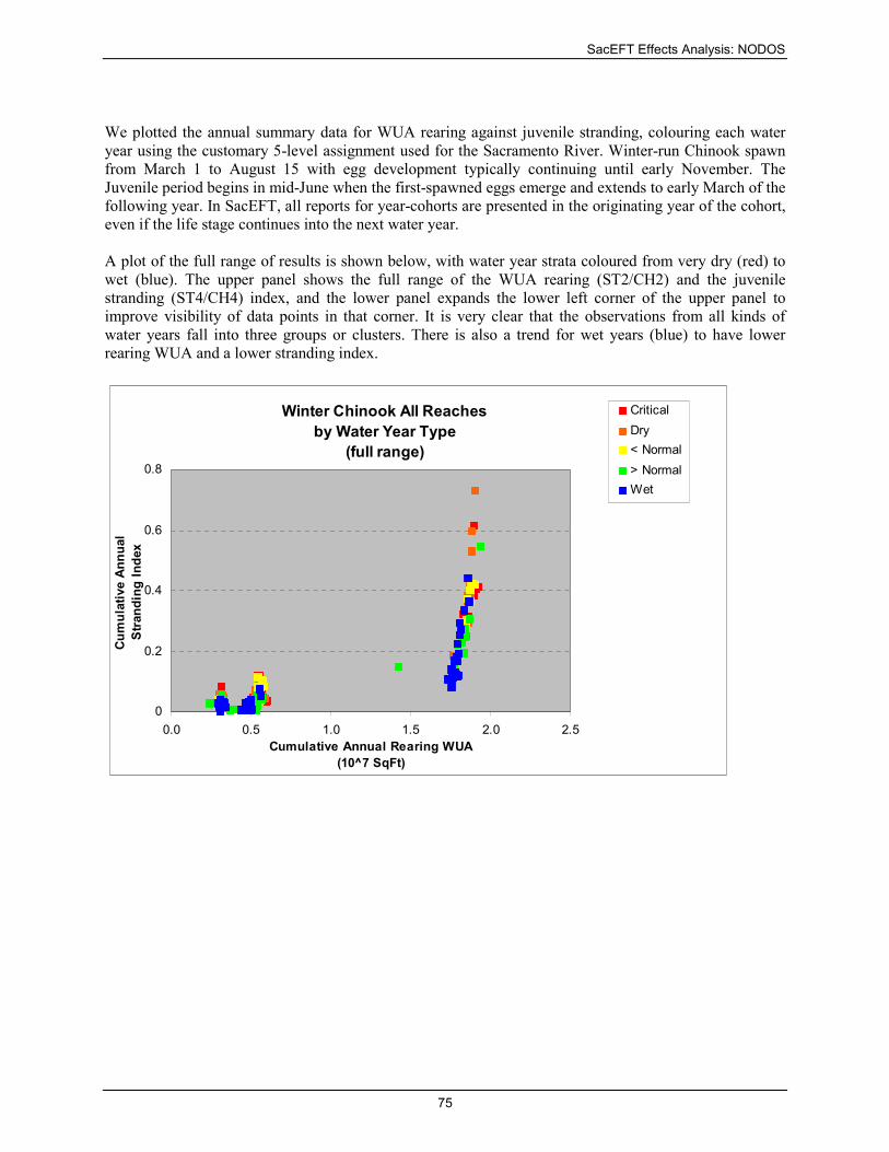
We plotted the annual summary data for WUA rearing against juvenile stranding, colouring each water
year using the customary 5-level assignment used for the Sacramento River. Winter-run Chinook spawn
from March 1 to August 15 with egg development typically continuing until early November. The
Juvenile period begins in mid-June when the first-spawned eggs emerge and extends to early March of the
following year. In SacEFT, all reports for year-cohorts are presented in the originating year of the cohort,
even if the life stage continues into the next water year.
A plot of the full range of results is shown below, with water year strata coloured from very dry (red) to
wet (blue). The upper panel shows the full range of the WUA rearing (ST2/CH2) and the juvenile
stranding (ST4/CH4) index, and the lower panel expands the lower left corner of the upper panel to
improve visibility of data points in that corner. It is very clear that the observations from all kinds of
water years fall into three groups or clusters. There is also a trend for wet years (blue) to have lower
rearing WUA and a lower stranding index.
Winter Chinook All Reaches
by Water Year Type
(full range)
0
0.2
0.4
0.6
0.8
0.0 0.5 1.0 1.5 2.0 2.5
Cumulative Annual Rearing WUA
(10^7 SqFt)
Cum
ula
tive A
nnual
Str
andin
g Index
Critical
Dry
< Normal
> Normal
Wet
SacEFT Effects Analysis: NODOS
76
Winter Chinook All Reaches
by Water Year Type
(for lower WUA values)
0
0.05
0.1
0.15
0.2
0.2 0.3 0.4 0.5 0.6 0.7 0.8
Cumulative Annual Rearing WUA
(10^7 SqFt)
Cum
ula
tive A
nnual
Str
andin
g Index
Critical
Dry
< Normal
> Normal
Wet
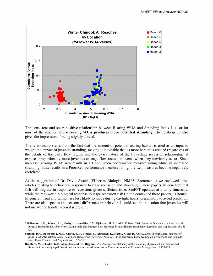
The different data cluster groups correspond to very different amounts of rearing WUA (x-axis) and to a
lesser extent stranding index (y-axis) in the 5 reaches which are modelled by SacEFT’s steelhead and
Chinook submodels. This is made clear in the results stratified by location, plotted below.
Winter Chinook All Reaches
by Location
(full range)
0
0.2
0.4
0.6
0.8
0.0 0.5 1.0 1.5 2.0 2.5
Cumulative Annual Rearing WUA
(10^7 SqFt)
Cum
ula
tive A
nnual
Str
andin
g Index
Reach 6
Reach 5
Reach 5
Reach 3
Reach 2
Reach 5 (which begins downstream from Battle Creek and is coloured orange in the upper panel) has
more than three times the potential rearing habit of the other reaches. The upper boundary of Reach 6 is at
Keswick and the lower boundary of Reach 2 is at Vina.
SacEFT Effects Analysis: NODOS
77
Winter Chinook All Reaches
by Location
(for lower WUA values)
0
0.05
0.1
0.15
0.2
0.2 0.3 0.4 0.5 0.6 0.7 0.8
Cumulative Annual Rearing WUA
(10^7 SqFt)
Cum
ula
tive A
nnual
Str
andin
g Index
Reach 6
Reach 5
Reach 5
Reach 3
Reach 2
The consistent and steep positive relationship between Rearing WUA and Stranding Index is clear for
most of the reaches: more rearing WUA produces more potential stranding. The relationship also
gives the impression of being slightly curved.
The relationship stems from the fact that the amount of potential rearing habitat is used as an input to
weight the impact of juvenile stranding, making it inevitable that as more habitat is created (regardless of
the details of the daily flow regime and the exact nature of the flow-stage recession relationship) it
exposes proportionally more juveniles to stage-flow recession events when they inevitably occur. Since
increased rearing WUA area results in a Good/Green performance measure rating while an increased
stranding index results in a Poor/Red performance measure rating, the two measures become negatively
correlated.
At the suggestion of Dr. David Swank (Fisheries Biologist, NMFS, Sacramento) we reviewed three
articles relating to behavioral responses to stage recession and stranding.1 These papers all conclude that
fish will migrate in response to recession, given sufficient time. SacEFT operates at a daily timescale,
while the real-world biological response to stage recession risk (in the context of these papers) is hourly.
In general, trout and salmon are less likely to move during daylight hours, presumably to avoid predation.
There are also species and seasonal differences in behavior. I could see no indication that juveniles will
not use wetted habitat when it is present.
1 Halleraker, J.H., Saltveit, S.J., Harby, A., Arnekliev, J.V., Fjeldstad, H.-P. And B. Kohler. 2003. Factors influencing stranding of wild
juvenile Brown trout (Salmo trutta) during rapid and frequent flow decreases in an artificial stream. River Research and Applications 19:589-
603.
Scruton, D.A., Ollerhead, L.M.N., Clarke, K.D., Pennell, C., Alfredsen, K., Harby, A. and D. Kelley. 2003. The behavioral response of
juvenile Atlantic salmon (Salmo salar) and Brook trout (Salvelinus fontinalis) to experimental hydropeaking on a Newfoundland (Canada) river. River Research and Applications 19:577-587.
Bradford, M.J., Taylor, G.C., Allan, J.A. and P.S. Higgins. 1995. An experimental study of the stranding of juvenile Coho salmon and Rainbow trout during rapid flow decreases in winter conditions. North American Journal of Fisheries Management 15:473-479.
SacEFT Effects Analysis: NODOS
78
Dr. Swank suggested that we might find some gauges with hourly (or shorter) stage measurements and
see how the high-resolution values are distributed, then compare that distribution to our daily resolution
data, creating a relationship between daily recession and the distribution of hourly recession. It might then
be possible to link the probability of a high-resolution rapid recession rate (e.g., exceeding 10cm hr–1 as a
threshold for “high risk”) derived from the literature with our daily recession. This could be a fairly
involved analysis, and our modelers do not believe it would fundamentally remove the inverse correlation
since the (potentially more accurate) hourly risk would still be weighted by rearing WUA in our model.
This page intentionally left blank.
SacEFT Effects Analysis: NODOS
79
Appendix B – Indicator Thresholds and Rating System1
The SacEFT output interface makes extensive use of a “traffic light” paradigm that juxtaposes
performance measure (PM) results and scenarios to provide an intuitive overview of whether a given
year’s PMs are experiencing favorable conditions (Green), are performing only fairly (Yellow), or are
experiencing unfavorable conditions (Red). For all twelve (12) performance measures, annual cumulative
weighted performance measure values are calculated for our default historical water operation scenario
based on the 66-year historical time series of observed flows and water temperatures from 1938 to 2003.
These “annual roll-up” values for each performance measure (e.g., average over days and locations with
applicable biological distributions) are then assigned a “good” (Green), “fair” (Yellow) or “poor” (Red)
performance measure rating (e.g., Figure B.1). The default threshold boundaries between Yellow/Green
and Red/Yellow are based on tercile break points determined by sorting the annual weighted performance
measure values from the default historical water operation scenario.
Figure B.1: Typical SacEFT output showing annual roll-up results for the Fremont cottonwood initiation (FC1)
performance measure. Analogous plots are available for all of the tools’ focal species and performance
measures.
These annual performance measure ratings are based on thresholds2 defined by sorting cumulative annual
results produced by SacEFT for historic observed flows and water temperatures between calendar years
1938 and 2003 (e.g., Figure B.2). The “units” of these plots vary with the performance measure. In this
way, historic observed flows/temperatures provide the de facto “calibration scenario” for SacEFT’s
twelve (12) focal species performance measures.
1 This introduction is drawn verbatim from Section 3.1.2 of:
ESSA Technologies Ltd. 2011. Sacramento River Ecological Flows Tool (SacEFT): Record of Design (v.2.00). Prepared by ESSA
Technologies Ltd., Vancouver, BC for The Nature Conservancy, Chico, CA. 111 p. + appendices.
2 Indicator thresholds in SacEFT are fully configurable via settings found in the SacEFT relational database.
SacEFT Effects Analysis: NODOS
80
SacEFT - Riparian Initiation (FC1) Calibration
7
99
53
36
0
20
40
60
80
100
1983
1958
1941
1969
2003
1998
1956
1982
2004
1963
1973
1999
1980
1965
1989
1993
1976
1957
1970
1988
1946
1979
1961
1960
1986
1985
1964
1949
1962
1948
1945
1950
1944
Water Year (Historical Flows)
# nodes w
surviving
cottonwood
seedlings
over all
cross
sections
Figure B.2: Annual roll-up results for the SacEFT Fremont cottonwood initiation (FC1) performance measure run
using historic observed flows (1938–2003). This calibration also takes into consideration comparisons
with aerial photographs of historically strong Cottonwood recruitment at study sites vs. model results.
Our concept of indicator threshold calibration in SacEFT focuses on historical data. From an ecological
standpoint, aquatic and riparian species are adapted to a historical range and frequency of variations in
their habitats. Taken to the extreme, historical conditions would ideally include pre-settlement (natural)
flows/water temperatures that represented ‘typical’ conditions experienced over evolutionarily significant
windows of time. The closest flow/temperature time series that we have available to this evolutionarily
representative condition is the range of variation in historical observed flows/temperatures (approximately
66 years). It is recognized that during 1938–2003 the Sacramento River experienced a number of waves
of human and structural development and operational changes to the hydrosystem. Nevertheless, these
flows and temperatures, derived from measurements, actually occurred in recent history and encompass
repeat episodes of multiple water year types. Calibrating SacEFT indicator thresholds to a future no action
or ‘existing’ scenario that includes a fixed set of hydrosystem features, constraints, operating regulations
and assumed human demands would create a “self-fulfilling prophecy” inconsistent with SacEFT’s
underlying natural flow regime science foundation. In general, all of the models used in the NODOS
investigation are calibrated based upon historical information.
Typically, none of the NODOS investigation project alternative modelling results are compared against
the historical calibration due to the focus of CEQA/NEPA which emphasizes isolating project alternative
effects as compared to a no action reference or existing condition comparison. Comparisons that include
historical data reveal different information in a different context that does not address a specific project
effect relative to the no action alternative or existing condition reference case. Comparisons that include
historic calibration data identify the ecological effects of the future system operations and constraints
relative to historic conditions. In fully considering ecological flow needs, the magnitude of departure from
SacEFT Effects Analysis: NODOS
81
these historic conditions may reveal important information on how future constraints, climate and/or
hydrosystem operational modifications are influencing preferred ecological flow targets.
The highest level synthesis concept in SacEFT is that of a “multi-year roll-up”. This is the percentage of
years in the simulation having favorable (Green), fair (Yellow), and poor (Red) conditions (e.g.,
Figure 2.3).
Figure B.3: Typical SacEFT output showing multi-year roll-up results for the Fremont cottonwood initiation (FC1)
performance measure. Analogous plots are available for all of the tools’ focal species and performance
measures.
The preferred method for calibrating the indicator thresholds is to identify historical years for each
performance measure that were known (in nature) to have experienced ‘good’ or ‘poor’ performance.
Unfortunately, our repeat survey efforts of fisheries experts (e.g., Mark Gard, USFWS, pers. comm.2011;
Matt Brown, USFWS, pers. comm. 2011 amongst many others) and a questionnaire sent to fisheries
biologists prior to the 2008 SacEFT v.1 review workshop revealed there are no known synoptic studies of
this kind for many of the indicators in SacEFT. Because of this gap and the hesitancy of experts to reveal
their opinions, we instead defaulted to the distribution of sorted weighted annual results and selected
tercile break-points (the lower-, middle- and upper thirds of the sorted distribution) to categorize results
into “Good” (Green), “Fair” (Yellow) or “Poor” (Red) categories. While this method provides a fully
internally consistent method of comparing scenario results (i.e., will always provide an accurate
picture of which water management scenarios are “better” than another), it does not necessarily
provide a concrete inference about the biological significance of being a “Poor” (Red) or “Good”
(Green) category. For example, it is possible that a year that ranks as “Good” (Green) with this method
may still be biologically suboptimal. Conversely, a year that ranks as “Poor” (Red) may be biologically
insignificant (i.e., not biologically ‘unacceptable’).
The challenge of identifying “acceptable” and “unacceptable” changes in habitat conditions or focal
species performance measures confronts all biological effects analysis methods. SacEFT makes these
inherent value judgments explicit in the model’s summary outputs. Future analyses using SacEFT look
forward to ecological effects analysis experts themselves providing clearer guidance on the (readily
configurable) thresholds in the SacEFT modeling system.
On the following pages, Table B.1 provides all indicator rating threshold values for the Daily and Annual
Rollup indicators. These are drawn from indicator threshold calibration descriptions in ESSA
Technologies (2011). In Table B.1, we flag cases where there are major gradients in performance
indicator thresholds. For detailed information on these thresholds, readers should refer to ESSA
Technologies (2011).
SacEFT Effects Analysis: NODOS
82
Table B.1: Indicator rating threshold breakpoints for the 12 Performance Measures found in SacEFT Version 2.
For detailed information on these thresholds, readers should refer to ESSA Technologies (2011).