1 Appendix A – Frequently Asked Questions (FAQs) Table of Contents FAQ #1: What are mass points, breaklines, TINs, and Terrains? ........................................................ 2 FAQ #2: What are digital elevation models (DEMs)?......................................................................... 3 FAQ #3: What is the difference between a digital terrain model (DTM) and a digital surface model (DSM)? ............................................................................................................................................ 5 FAQ #4: What is the difference between a DTM and a TIN? ............................................................ 5 FAQ #5: How are DEMs produced from imagery/photogrammetry, IFSAR and LiDAR? ..................... 6 FAQ #6: What is a LiDAR point cloud? ............................................................................................ 12 FAQ #7: What is a LiDAR cross-section? ......................................................................................... 13 FAQ #8: What is the difference between DEM post spacing and nominal pulse spacing (NPS)? ...... 13 FAQ #9: What is the difference between RMSEz, equivalent contour accuracy, and other terms used to describe vertical accuracy? ........................................................................................................ 14 FAQ #10: How do I determine what DEM post spacing or nominal pulse spacing (NPS) I need? ...... 15 FAQ #11: What is the difference between hydro-flattening and hydro-enforcement? .................... 19 FAQ #12: What are hillshades? ...................................................................................................... 22 FAQ #13: What are elevation derivatives?...................................................................................... 23 FAQ #14: How frequently does elevation data need to be updated? .............................................. 24 FAQ #15: What is the National Elevation Dataset (NED)? ............................................................... 30 FAQ #16: What is the Center for LiDAR Information Coordination and Knowledge (CLICK)?............ 31 FAQ #17: What are Elevation Derivatives for National Applications (EDNA)? .................................. 32 It is important for respondents to the questionnaire to understand the answers to the 17 FAQs explained, with graphic examples, below. The terms explained herein must be understood in order to provide valid responses to questions pertaining to user elevation data requirements and benefits.
Transcript
1
Appendix A – Frequently Asked Questions (FAQs)
Table of Contents
FAQ #1: What are mass points, breaklines, TINs, and Terrains? ........................................................ 2
FAQ #2: What are digital elevation models (DEMs)?......................................................................... 3
FAQ #3: What is the difference between a digital terrain model (DTM) and a digital surface model
Today, some combination of mass points, breaklines, TINs and/or Terrains are used to produce DEMs.
FAQ #2: What are digital elevation models (DEMs)?
As used in this questionnaire, a Digital Elevation Model (DEM) is a grid of bare-earth z-values at regularly
spaced intervals in x and y directions. For national datasets, x and y may be best defined on a spherical
reference surface in terms of longitude and latitude. For smaller datasets, x and y are normally defined
on a planar (flat) reference surface, normally using Universal Transverse Mercator (UTM) or State Plane
coordinates. For entry into the NED, USGS converts data with UTM or State Plane coordinates into DEMs
with arc-second post spacing. Whereas traditional contours are still used by some for manual, visual
interpretation of the topographic surface, today’s DEMs are widely used for a large variety of
automated analyses, mathematical models, and 3D simulations and visualizations.
For DEMs in the NED, DEM post spacing (grid spacing) is defined in geographic coordinate angular units
on a spherical surface. Figure 7 shows ∆x and ∆y in arc-seconds of longitude and latitude, best for a
national dataset with multiple “nested” resolutions as used with the National Elevation Dataset (NED).
Figure 3. Example of a Terrain showing TIN triangles. Figure 3. Example of a Terrain showing TIN triangles.
4
For smaller elevation datasets produced for states and counties for example, DEM post spacing is
normally alternatively defined in metric units on a planar surface. Figure 8 shows ∆x and ∆y in meters for
either UTM or State Plane Coordinate System (SPCS) georeferencing.
Originally, DEMs were interpolated from contours; but today, most contours are produced from DEMs,
supplemented with breaklines to make them aesthetically pleasing, as shown at Figure 9. Today’s DEMs
are produced from LiDAR, stereo imagery, or IFSAR.
Figure 7. ∆x and ∆y in arc-seconds of longitude and latitude used w/NED
Figure 8. ∆x and ∆y in feet or meters used w/UTM or State Plane system
Figure 9. Contours produced from DEM
using hydro and road breaklines
When looking closely at how DEMs are stored, they are seen to be extremely efficient.
DEMs can be viewed as pixels, color-coded by elevation, as shown at Figure 10. DEMs have small file sizes because x/y incrementation by ∆x and ∆y eliminates the need for storing individual x/y coordinates, as shown at Figure 11.
Figure 10. DEM viewed as pixels, color-
coded by elevation
Figure 11. DEM files are small and
efficient because individual x/y coordinates do not need to be stored
5
FAQ #3: What is the difference between a digital terrain model (DTM) and a digital surface
model (DSM)?
A Digital Terrain Model (DTM) is an elevation
model of the bare earth terrain surface, but
normally with irregularly-spaced points rather than
the uniform grid structure of a DEM. A DTM often
includes breaklines to help define edges of TIN
triangles. See bottom of Figure 12. A hydro
breakline could be added here to enforce the
downward flow of water in the drainage feature.
A Digital Surface Model (DSM) is an elevation
model of the top reflective surface, including the
bare earth in open terrain areas, as well as the
tops of buildings, trees, towers, and other features
elevated above the bare earth. See top of Figure
12.
Figure 12. DSM of top reflective surface and DTM of bare-earth terrain beneath the vegetation.
FAQ #4: What is the difference between a DTM and a TIN?
A Digital Terrain Model (DTM) generally refers to an irregular surface of elevations represented with
discreet masspoints measured by LiDAR or photogrammetric means and may also contain vector
breaklines. A DTM is generally represented in a vector, ascii or binary format. DTMs are easily tiled
within exact tile boundaries.
A Triangulated Irregular Network (TIN) is a data structure used to represent a ground surface model like
a DEM or DTM. A TIN usually contains the same masspoints and/or breaklines as a DTM. However, the
TIN data structure also contains a topological component by which discreet points and vertices are
connected through a series of triangles, each triangle having its own slope and aspect. Each triangle
creates a unique facet in the ground surface model and these facets are extremely useful for visualizing
and analyzing slope, aspect, cut and fill of the terrain, and they are used for interpolation of gridded
elevation posts and for generation of contours. A TIN’s file size is normally between 2X and 4X larger
than a DTM covering the same area with the same masspoints and breaklines. It is more difficult to tile a
TIN because TIN triangles normally cross over tile boundaries.
Figure 13 shows a geometric view of TIN triangles; each triangle maintains topological data structure
with all adjoining TIN triangles. Figure 14 shows a surface view of this TIN, with interpolated contours.
Each TIN triangle has its own slope and aspect. These triangles are interpolated at X/Y coordinates of
DEM posts to determine the elevation of each post; a DTM cannot do this. TIN triangles are also
interpolated to determine contour lines of equal elevation that cross these TIN triangles; a DTM cannot
do this either.
6
Figure 13. Geometric view of TIN with topological data
structure, showing individual TIN triangles
Figure 14. Surface view of TIN with derived contours. DEM
elevation posts are interpolated from TIN triangles
FAQ #5: How are DEMs produced from imagery/photogrammetry, IFSAR and LiDAR?
Gridded DEMs are produced at mathematically-computed x and y coordinates by interpolation on TIN
triangles produced from irregularly-spaced mass points surrounding each point to be interpolated. The
most important points to understand about these technologies are the following:
Photogrammetry
Photogrammetry requires stereo views of the terrain from two different perspectives. If both views
cannot see the bare earth terrain beneath the trees, then photogrammetry cannot map the elevations
of the bare earth. This is why photogrammetry is well suited for open terrain but ill suited for mapping
of vegetated areas. Figures 15 and 16 shows how stereo views are obtained from traditional frame
cameras (digital and film) and from new push-broom sensors.
Figure 15. Frame cameras (digital and film) obtain stereo images by having at least 60% overlap between photos so that all areas are imaged from two perspectives
Figure 16. Push-broom sensors obtain stereo views by collecting forward and backward views for automated DSM/DTM production, plus downward view for digital orthophotos.
7
Photogrammetry is rarely used today for the sole
purpose of generating DEMs, DSMs, DTMs or
contours. However, airborne imagery is routinely
acquired with forward overlap of 60% or more for
production of digital orthophotos nationwide; this
normally requires some form of aerial
triangulation (AT). The 60% overlap creates stereo
images required for all forms of photogrammetry
(Figure 17), including manual photogrammetry
(Figure 18) and automated photogrammetry
(Figure 19) that can be used to produce DEMs.
Without acquisition of any new imagery, existing
imagery and AT solutions from orthophoto
programs also can be used for DEM production.
DEM accuracy (between 2.5 and 15 foot
equivalent contour accuracy) depends on the
flying height and rigor of the AT processes used.
Figure 17. For any point to be mapped photogrammetrically, it must be visible on stereo images, both images seeing the same point P from two different perspectives (at P1 and P2). In this Figure, O1 and O2 are the locations of the camera’s focal point when the two images were taken. Because trees normally block stereo views, it is difficult to map the bare earth terrain in vegetated areas using photogrammetry.
Figure 18. With manual photogrammetry, the compiler uses polarized glasses to see the left image with the left eye and the right image with the right eye, manually compiling spot heights where the bare earth terrain is visible in stereo and/or compiling 3D breaklines. Manually compiled contours are considered too expensive and time-consuming.
Figure 19. With automated photogrammetry, the computer correlates image pixels on stereo images and computes uniformly-spaced grid points that are initially DSM points of the top reflective surface. Semi-automated processes are then used to reclassify non-ground points so as to retain only the bare-earth DTM grid points (shown in green).
Table 1 summarizes the DEM accuracy achievable from imagery already acquired for production of
digital orthophotos at various pixel resolutions, including 1-meter images for the National Agriculture
Imagery Program (NAIP). Imagery and AT data would need to be preserved for re-use.
Table 1. How existing stereo imagery can be re-used to produce DEMs
Current Owner of Existing Imagery/AT
Orthophoto Pixel Resolution
Typical Flying Height above Terrain
Equivalent Contour Accuracy Achievable
Typical Vertical RMSEz
USGS/state/local 6-inch 4,800 feet 2.5 foot 23.2 cm
USGS/state/local 1-foot 9,600 feet 5 foot 46.3 cm
USDA (NAIP) 1-meter 30,000 feet 15 foot 1.39 meter
8
Interferometric Synthetic Aperture Radar (IFSAR)
Airborne IFSAR is acquired from approximately 35,000 feet above mean terrain, covering very large
areas. X-band IFSAR, which maps the top reflective surface, is primarily used in the U.S. because other
bands often interfere with communications and require special permissions for acquisition. Figure 20
shows an IFSAR DSM and Figure 21 shows an IFSAR DTM. Figure 22 shows the ortho-rectified radar
image (ORI) of the same area; ORIs create masks of water areas that assist with hydrographic feature
extraction and interpretation of data when producing hydro-enforced DTMs. Figure 23 shows the side-
looking geometry used with IFSAR data collection; this geometry sometimes causes data voids caused by
overlay, shadow and foreshortening, explained in the IFSAR chapter of the 2nd edition of “Digital
Elevation Model Technologies and Applications: The DEM Users Manual,” published by ASPRS; closer
flight line spacing and different look angles are used to minimize this problem in mountainous terrain.
Although not in the public domain, existing airborne IFSAR is currently available and licensed for all
states except Alaska.
Figure 20. IFSAR collects the top reflective surface used to produce a digital surface model (DSM)
Figure 21. The IFSAR DSM is subsequently filtered to produce a digital terrain model (DTM)
Figure 22. IFSAR ortho-rectified radar image (ORI) used to generate water masks, eliminating need for breaklines
Figure 23. IFSAR maps to the side of the aircraft using principles of interferometry, but can create data voids from foreshortening, layover and shadow
9
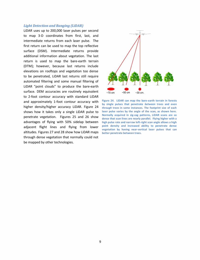
Light Detection and Ranging (LiDAR)
LiDAR uses up to 200,000 laser pulses per second
to map 3-D coordinates from first, last, and
intermediate returns from each laser pulse. The
first return can be used to map the top reflective
surface (DSM). Intermediate returns provide
additional information about vegetation. The last
return is used to map the bare-earth terrain
(DTM); however, because last returns include
elevations on rooftops and vegetation too dense
to be penetrated, LiDAR last returns still require
automated filtering and some manual filtering of
LiDAR “point clouds” to produce the bare-earth
surface. DEM accuracies are routinely equivalent
to 2-foot contour accuracy with standard LiDAR
and approximately 1-foot contour accuracy with
higher density/higher accuracy LiDAR. Figure 24
shows how it takes only a single LiDAR pulse to
penetrate vegetation. Figures 25 and 26 show
advantages of flying with 50% sidelap between
adjacent flight lines and flying from lower
altitudes. Figures 27 and 28 show how LiDAR maps
through dense vegetation that normally could not
be mapped by other technologies.
Figure 24. LiDAR can map the bare-earth terrain in forests by single pulses that penetrate between trees and even through trees in some instances. The footprint size of each laser pulse varies by the angle of the scan, as shown here. Normally acquired in zig-zag patterns, LiDAR scans are so dense that scan lines are nearly parallel. Flying higher with a high pulse rate and narrow left-right scan angle allows a high point density and increased ability to penetrate dense vegetation by having near-vertical laser pulses that can better penetrate between trees.
10
Figure 25. Flying with 50% sidelap between adjoining flight lines doubles the point density, increases the probability of penetrating dense vegetation by having two look directions from different perspectives, and provides alternative elevation points when a single swath includes high intensity returns that cause “trenching” and need to be eliminated from the dataset.
Figure 26. Vertical accuracy decreases with increased flying height, but costs can be reduced by flying form higher altitudes with higher point density.
Figure 27. In spite of dense vegetation shown on this orthophoto in Florida, LiDAR data collected at a point density of 4 points/m2 was still able to establish a hydro flow line for the dry drainage feature beneath.
Figure 28. Color-coded by 1-foot contour elevation bands, the white polygons define depression contours that show dry puddles that should not normally be hydro-enforced (defined below).
LiDAR raw point cloud data are normally classified in the standard LAS file format using class 1
(processed, but unclassified), class 2 (bare-earth ground), class 7 (noise) and class 9 (water). Other LAS
classes are used but beyond the scope of this questionnaire.
LiDAR also produces intensity images that record the intensity of return from each laser pulse. Intensity
images are used with lidargrammetry for compilation of 3D breaklines. Figures 29 and 30 show
examples of intensity images that include teaching points.
11
Figure 29. Intensity image showing streaks over water from multiple flight lines. This is not a problem because LiDAR measurements on water are already assumed to be unreliable and are classified separately as LAS Class 9. This entire image is usable for lidargrammetry.
Figure 30. High intensity streaks over land and marshy areas can be problematic because high intensity returns cause “trenches” where elevations are mapped lower than their true elevation. The top image maps the different intensity values along the cross-section shown in the lower image.
LiDAR point cloud data is processed to ASPRS LAS classes that distinguish between points on the ground,
water, or elevated features such as buildings, trees, towers, bridges, etc. No points are discarded but
may be classified as noise, or unclassified. All elevations in water are unreliable because sometimes the
laser pulses are absorbed by the water, reflected from the water with differing intensities as shown
above, or provide elevations on or below the level of the water surface. Most LiDAR data is flown with
the laser scanning in a zig-zag pattern where the zigs and zags are so close that they appear to be
parallel. The objective is to obtain pulse spacing and flight speed so that the nominal pulse spacing
(NPS) is approximately equal in the in-flight and cross-flight directions.
It is normal for LiDAR elevation posts to appear to be
noisy. However, in misguided attempts to smooth the
terrain surface, analyses sometimes over-smooth and
remove steep slopes that actually exist. Figure 31 is
an example of over-smoothing, as demonstrated by a
man-made channel that was constructed with the
same cross-section dimensions throughout its length.
The area on the left appears noisy, but the cross-
section profile accurately shows the drainage channel
to be about 50 feet wide with steeper slopes. The
area on the right is seen to be smoother and more
aesthetically pleasing; however, the cross-section
profile incorrectly shows the drainage channel to be
about 150 feet wide with shallower banks. For some
applications, users prefer smoother terrain, but for
hydraulic modeling and other applications, users need to know actual cross-section dimensions. It is
normal for QA/QC reviews to test for over-aggressive smoothing.
Figure 31. Although it appears noisy, the area on the left preserved the true shape of the man-made drainage channel, whereas the smoothed area on the right over-smoothed the shape of the same drainage channel, making it much wider and shallower.
12
All Technologies
The most important thing to remember about DEM production is that DEMs are interpolated from
source data of higher density than the uniform post spacing of the DEM being produced. For example:
DEMs with 1-meter (or 1/27-arc-second) post spacing are produced from elevation data with
nominal pulse spacing (NPS) typically between 0.35 and 0.7 meters.
DEMs with 3-meter (or 1/9-arc-second) post spacing are produced from elevation data with NPS
typically between 1.0 and 2.0 meters. This is consistent with USGS LiDAR Guidelines and Base
Specifications, v13.
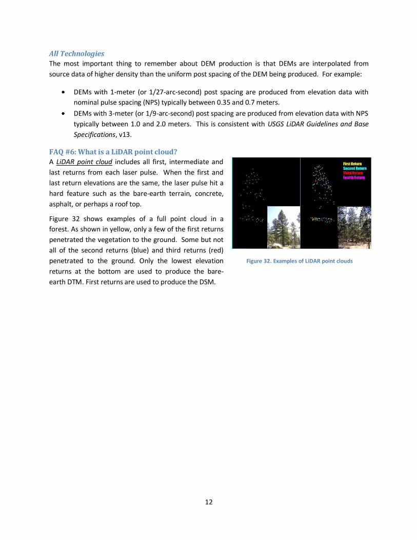
FAQ #6: What is a LiDAR point cloud?
A LiDAR point cloud includes all first, intermediate and
last returns from each laser pulse. When the first and
last return elevations are the same, the laser pulse hit a
hard feature such as the bare-earth terrain, concrete,
asphalt, or perhaps a roof top.
Figure 32 shows examples of a full point cloud in a
forest. As shown in yellow, only a few of the first returns
penetrated the vegetation to the ground. Some but not
all of the second returns (blue) and third returns (red)
penetrated to the ground. Only the lowest elevation
returns at the bottom are used to produce the bare-
earth DTM. First returns are used to produce the DSM.
Figure 32. Examples of LiDAR point clouds
13
FAQ #7: What is a LiDAR cross-section?
LiDAR cross-sections, also called transects, are
profiles “cut” through LiDAR point clouds in order
to visualize or measure heights or elevation
differences in points collected along those cross-
sections. Figure 33 shows an example of a LiDAR
cross-section cut across a river, to include elevation
data on a bridge as well as elevations of bare-earth
terrain, vegetation and buildings on either side of
the river.
Figure 33. Digital orthophoto (lower image) shown with location of cross-section cut in LiDAR data. The upper image shows the elevations of all features along this cross-section.
FAQ #8: What is the difference between DEM post spacing and nominal pulse spacing (NPS)?
Within the NED, DEM post spacing is uniformly-spaced, but as a fraction of an arc-second (see Figure 7, above). DEM post spacing outside the Federal government is normally uniformly-spaced, usually as some whole integer value of meters, e.g., 1, 2, 5 or 10 meters (see Figure 8, above).
Nominal pulse spacing (NPS) refers to the average point spacing of a LiDAR dataset typically acquired in a zig-zag pattern with variable point spacing along-track and cross-track. NPS is an estimate and not an exact calculation; standard procedures are under development by ASPRS for NPS calculations.
Figure 34 shows high density NPS in red (left) and low density interpolated DEM posts (right).
Figure 34. Higher density, irregularly-spaced LiDAR mass points (red) are used to interpolate the lower density DEM grid points shown on the right. Several hydro breaklines are also shown in this image.
For USGS acceptance, the spatial distribution of geometrically usable points is expected to be uniform and free from clustering. In order to ensure uniform densities throughout the data set, a regular grid, with cell size equal to the design NPS x 2 is laid over the data. At least 90% of the cells in the grid must contain at least 1 LiDAR point. NPS assessment is made against single swath, first return data located within the geometrically usable center portion (typically ~90%) of each swath. Average along-track and cross-track point spacing should be comparable. Point density and NPS comparisons are shown here.
Point Density NPS
8 pt/m2 0.354 m 6 pt/m2 0.408 m
4 pt/m2 0.500 m
2 pt/m2 0.707 m 1 pt/m2 1.0 m
0.25 pt/m2 2.0 m
0.04 pt/m2 5.0 m
14
Instead of flying with a minimal side lap of 10%, many firms now acquire their LiDAR data with 50% side lap, as shown at Figure 35. This minimizes the risk of having gaps in data between flight lines caused by excessive roll and pitch of the aircraft during windy conditions; and this increases the probability of penetrating dense vegetation by having two different look angles, as also shown at Figure 35. A side lap of 50% doubles the average point density compared with single swaths.
Figure 35. Comparison between 10% and 50% side lap between overlapping LiDAR swaths
FAQ #9: What is the difference between RMSEz, equivalent contour accuracy, and other
terms used to describe vertical accuracy?
For decades, contour lines were developed for human interpretation of elevations on printed
topographic maps, and the contour interval defined the map’s vertical accuracy. The contour interval
had a specific meaning for satisfaction of the National Map Accuracy Standard (NMAS), i.e., not more
than 10 percent of the elevations tested may be in error more than one-half the contour interval. In
other words, 90 percent or more of errors should be equal to or less than one-half the contour interval.
Contour lines can be produced today from DEMs and digital elevation data with virtually any contour
interval, but this would be misleading if it falsified the vertical accuracy of the elevation data from which
the contours were derived. In 1998, the Federal Geographic Data Committee published the National
Standard for Spatial Data Accuracy (NSSDA) which implemented a statistical and testing methodology
for estimating the positional accuracy of points on maps and in digital geospatial data, with respect to
georeferenced ground positions of higher accuracy. The NSSDA specified that vertical accuracy be
specified in statistical terms at the 95% confidence level, defined as 1.9600 x RMSEz when errors follow
a normal error distribution. In 2004, recognizing that LiDAR DTM errors do not necessarily follow a
normal error distribution, the National Digital Elevation Program (NDEP) published its “Guidelines for
Digital Elevation Data” and the American Society for Photogrammetry and Remote Sensing (ASPRS)
published the “ASPRS Guidelines, Vertical Accuracy Reporting for Lidar Data.” The NDEP and ASPRS
guidelines both distinguished between Fundamental Vertical Accuracy (FVA) in open, non-vegetated
terrain, and Supplemental Vertical Accuracy (SVA) in individual land cover categories and Consolidated
Vertical Accuracy (CVA) in combined land cover categories. It is now common for LiDAR specifications to
require a higher vertical accuracy in open terrain (FVA) and a lower vertical accuracy in vegetated terrain
(for the SVA and CVA). Both the SVA and CVA allow the use of 95th percentile errors rather than errors
computed statistically at the 95% confidence level. Both the 95% confidence level and the 95th
percentile define vertical accuracy in terms of the vertical linear uncertainty such that the true or
theoretical location of the point falls within ± of that linear uncertainty value 95-percent of the time.
Consistent with NSSDA, NDEP and ASPRS guidelines, Table 2 compares the vertical RMSEz and vertical
accuracy at the 95% confidence level necessary for digital elevation data to have the equivalent contour
accuracy specified in the left column. Because most users are still confused by an RMSEz of 18.5 cm, for
example, or vertical accuracy of 36.3 cm at the 95% confidence level, the geospatial community
15
translates these terms into 2-ft equivalent contour accuracy, as demonstrated in Table 2 and for a range
of other common contour intervals. It must also be noted that contours, used for human visualization,
are in decreasing demand because of hillshades and other forms of 3-D visualization from digital
elevation data. Today, most terrain analyses are performed by computer analyses of DEMs or other
forms of digital elevation data for which contour lines, themselves, are meaningless.
Table 2. Equivalent Contour Accuracy for Common Statistical Accuracy Terms.
Equivalent
Contour
Accuracy
RMSEz NMAS Vertical Accuracy at
90% Confidence Level
NSSDA Vertical Accuracy at
95% Confidence Level
1-foot 9.25 cm (~0.3 ft) 0.5 ft 18.15 cm (~0.6 ft)
2-foot 18.5 cm (~0.6 ft) 1.0 ft 36.3 cm (~1.2 ft)
5-foot 46.3 cm (~1.5 ft) 2.5 ft 90.8 cm (~3.0 ft)
10-foot ~3 ft 5.0 ft ~6.0 ft
15-foot ~4.5 ft 7.5 ft ~9.0 ft
20 foot ~6 ft 10.0 ft ~12.0 ft
FAQ #10: How do I determine what DEM post spacing or nominal pulse spacing (NPS) I need?
The determination of the minimal acceptable point density, DEM post spacing and/or NPS needed to
satisfy Business Uses is central to the purpose of this questionnaire. Respondents should not specify
requirements that are “nice to have” but focus instead on minimal acceptable requirements for
satisfaction of their Business Uses. Several considerations are suggested below, but ultimately this must
be the decision of elevation data users that best understand their technical requirements.
Five questions should be considered:
1. What level of detail do you need to see from the elevation data?
2. What are your needs for feature extraction?
3. What do you need to measure?
4. How dense is the vegetation you need to penetrate?
5. What are your needs for breaklines?
Consideration #1 (What you need to see). For some Business Uses, users need to be able to see certain
terrain features to be analyzed. The current DEM resolutions in the NED can be used for comparison
purposes. It is easier to see the visual effects of resolution than the visual effects of elevation accuracy.
Figure 36 shows a digital orthophoto of the Pecatonica River, in Winnebago, County, IL. The National
Elevation Dataset (NED) uses arc-second DEM post spacing, typically 1-arc-second (~30 meter spacing at
the Equator, see Figure 37), 1/3-arc-second spacing (~10 meter spacing at the Equator, see Figure 38),
and 1/9-arc-second spacing (~3 meter spacing at the Equator, see Figure 39). All three resolutions
shown have the same vertical accuracy, though their horizontal resolutions are very different.
16
Figure 36. Digital Orthophoto, Winnebago County, IL
Figure 37. DEM, 1-arc-sec (~30 meter post spacing)
Figure 38. DEM, 1/3-arc-sec (~10 meter post spacing)
Figure 39. DEM, 1/9-arc-sec (~3 meter post spacing)
If you can see what you need from the 1-arc-second (~30 meter) DEM at Figure 37, and if your
Business Use can accept DEMs produced for the NED from topographic quad maps that are
about 50 years old, the status quo may be acceptable. Then you probably have no Business Use
requirement for enhanced elevation data unless you also need DSMs.
If you can see what you need from the 1/3-arc-second (~10 meter) DEM at Figure 38, your
Business Use DEM needs may be satisfied by 10-meter NED data where it already exists,
produced from old topographic quad map source data. Elsewhere, you may need elevation data
(DSMs/DTMs) produced from IFSAR (Quality Level 4) or elevation data produced
photogrammetrically from existing imagery (Quality Level 3).
If you can see what you need from the 1/9-arc-second (~3 meter) DEM at Figure 39, but cannot
see what you need from the 1-arc-second or 1/9-arc-second DEM from the NED, your Business
Use probably needs elevation data produced from standard LiDAR (Quality Level 2).
USGS is now considering 1/27-arc-second DEM post spacing (~1 meter post spacing at the
Equator) as appropriate for gridded DEMs from LiDAR acquired with sub-meter NPS (Quality
Level 1). This Quality Level requires alternative consideration because it is difficult to visually
see the difference between a DEM with 3-meter, 2-meter and 1-meter post spacing.
17
Consideration #2 (Features you need to extract). A high resolution DEM is often required if
LiDAR data are to be used for automated or semi-automated feature extraction, as shown in
Figures 40 and 41.
Figure 40. Even with sub-meter NPS, building footprint edges are pixilated. Straight edges are difficult to define when they are irregular and pixilated.
Figure 41. High resolution elevation data are required when LiDAR is used for semi-automated feature extraction. Many misclassifications result from low resolution elevation data.
Consideration #3 (What you need to measure). Your DEM user application has everything to do with
required point density. Table 3, below, shows examples where measurements are made for landslides,
morphology, building classification, fire loads, tree species, forest metrics, vegetation classification, and
measurement of the DTM in the forest floor. Other applications might include assessment of forest
health.
Consideration #4 (Density of vegetation to be penetrated). In some cases, the raw LiDAR point density
per square meter or the NPS is much more important than the DEM post spacing, especially in areas of
dense vegetation. Figures 21 and 22 (see FAQ #5) show an example of LiDAR data in Florida where
LiDAR data was collected with an average density of 4 points/m2 in dense tropical vegetation. This
worked in Florida, but in the Pacific Northwest, 4 points/m2 may not be good enough for specific
applications.
A paper entitled, “Minimum LiDAR Data Density Considerations for the Pacific Northwest,” by
Watershed Sciences, Inc, 01/22/10, stated the following: “Not all pulses emitted from the laser will
measure the ground. Depending on vegetation and land cover, few pulses, and in some cases, no laser
pulses, will reach the ground. In order to relate pulse density to ground point density, a mathematical
relationship has been calculated from public-domain LiDAR surveys collected in Oregon in the last two
years. For these surveys, totaling over 5.2 million acres, a resolution of 8 pulses per square meter was
achieved. It was found that for any one pulse emitted, the probability of being classified as ground was
only 14%.” Analyses were performed to recommend pulses per square meter and NPS for different
applications used in the Pacific Northwest, as summarized in Table 3.
Table 3 addresses both considerations #3 and #4.
18
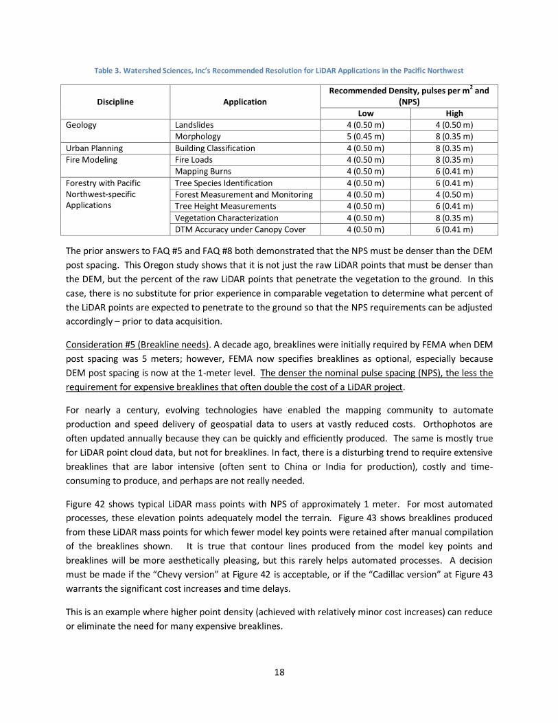
Table 3. Watershed Sciences, Inc’s Recommended Resolution for LiDAR Applications in the Pacific Northwest
Discipline Application Recommended Density, pulses per m
2 and
(NPS) Low High
Geology Landslides 4 (0.50 m) 4 (0.50 m)
Morphology 5 (0.45 m) 8 (0.35 m)
Urban Planning Building Classification 4 (0.50 m) 8 (0.35 m)
Fire Modeling Fire Loads 4 (0.50 m) 8 (0.35 m)
Mapping Burns 4 (0.50 m) 6 (0.41 m)
Forestry with Pacific Northwest-specific Applications
Tree Species Identification 4 (0.50 m) 6 (0.41 m)
Forest Measurement and Monitoring 4 (0.50 m) 4 (0.50 m) Tree Height Measurements 4 (0.50 m) 6 (0.41 m)
Vegetation Characterization 4 (0.50 m) 8 (0.35 m)
DTM Accuracy under Canopy Cover 4 (0.50 m) 6 (0.41 m)
The prior answers to FAQ #5 and FAQ #8 both demonstrated that the NPS must be denser than the DEM
post spacing. This Oregon study shows that it is not just the raw LiDAR points that must be denser than
the DEM, but the percent of the raw LiDAR points that penetrate the vegetation to the ground. In this
case, there is no substitute for prior experience in comparable vegetation to determine what percent of
the LiDAR points are expected to penetrate to the ground so that the NPS requirements can be adjusted
accordingly – prior to data acquisition.
Consideration #5 (Breakline needs). A decade ago, breaklines were initially required by FEMA when DEM
post spacing was 5 meters; however, FEMA now specifies breaklines as optional, especially because
DEM post spacing is now at the 1-meter level. The denser the nominal pulse spacing (NPS), the less the
requirement for expensive breaklines that often double the cost of a LiDAR project.
For nearly a century, evolving technologies have enabled the mapping community to automate
production and speed delivery of geospatial data to users at vastly reduced costs. Orthophotos are
often updated annually because they can be quickly and efficiently produced. The same is mostly true
for LiDAR point cloud data, but not for breaklines. In fact, there is a disturbing trend to require extensive
breaklines that are labor intensive (often sent to China or India for production), costly and time-
consuming to produce, and perhaps are not really needed.
Figure 42 shows typical LiDAR mass points with NPS of approximately 1 meter. For most automated
processes, these elevation points adequately model the terrain. Figure 43 shows breaklines produced
from these LiDAR mass points for which fewer model key points were retained after manual compilation
of the breaklines shown. It is true that contour lines produced from the model key points and
breaklines will be more aesthetically pleasing, but this rarely helps automated processes. A decision
must be made if the “Chevy version” at Figure 42 is acceptable, or if the “Cadillac version” at Figure 43
warrants the significant cost increases and time delays.
This is an example where higher point density (achieved with relatively minor cost increases) can reduce
or eliminate the need for many expensive breaklines.
19
Figure 42. LiDAR mass points with nominal pulse spacing
(NPS) of approximately 1 meter
Figure 43. Thinned model key points and breaklines for
swales, borrow pits with water, and road features
FAQ #11: What is the difference between hydro-flattening and hydro-enforcement?
Hydro-flattening is a relatively new term used by USGS to explain how DEMs are traditionally processed
for inclusion in the NED. Hydro-flattening is performed to depict the bare-earth terrain as one could see
and understand the terrain from an airplane flying overhead. The viewer would assume that the
surfaces of lakes and reservoirs are flat and that rivers are flat from shore to shore. The viewer would
also recognize that bridges are man-made features that should be removed from a bare-earth DTM
because they are artificially elevated above the natural terrain.
Figures 44 and 45 demonstrate how the shoreline elevations of lakes and reservoirs are flattened.
Figure 44. LiDAR mass points in this nearly-dry reservoir have variable elevations. It is difficult to identify the water shoreline or its flat elevation.
Figure 45. Special software is used to generate the breakline for the shoreline used to flatten the water surface elevation for this reservoir.
Figures 46 and 47 demonstrate how dual-line drainage features ≥ 100 feet in width are flattened from
shore to shore. Per USGS LiDAR Guidelines and Base Specifications, v13, these streams do not
necessarily have monotonic gradients that decrease as the river flows downstream, though this is
normally done anyhow in a process call hydro-enforcement. Gradients can be smooth (Figure 46) or
stair-stepped (Figure 47) so long as the height of the steps are not too steep and each step is flat from
shore to shore on either side of the river. Narrower rivers are depicted as single-line drainage features
that do not require flattening but may require hydro-enforcement.
20
Figure 46. Hydro flattened dual-line stream (top) with a smooth gradient (bottom). Top image also shows bridge removed from the DEM.
Figure 47. Hydro flattened dual-line stream (top) with a stair-stepped gradient (bottom). Each stair step in this example is 10 cm high (– 4 inches).
Figures 48 and 49 demonstrate how all bridges over such rivers, recognized as man-made features
constructed above the bare earth terrain, are removed from the DEM; but with hydro-flattening, below-
ground culverts are not “cut” to allow water to pass under the road.
Figure 48. Elevations on the bridge are removed to allow mapping and flattening of the river beneath the bridge. The underground culvert is not cut, artificially diverting the flow along the north side of the road until reaching the river.
Figure 49. This shows an oblique view of a digital image draped over the hydro-flattened DEM from the prior Figure. The bridge deck is lowered to the elevation of the ground beneath. The culvert on the right is clearly visible.
21
Hydro-enforcement includes hydro-flattening, as defined by USGS, but includes additional steps for
treatment of dual-line and single-line streams to enforce the downward flow of water. Figures 50 and
51 are commonly used as examples of how to hydro-enforce a dual-line stream that appears to block
the flow of water in the TIN shown at Figure 50 but enforces the downward flow of water in the hydro-
enforced TIN at Figure 51.
Figure 50. Rocks in the river, and/or natural undulating elevations along the shorelines, make the TIN appear as though water cannot pass downstream.
Figure 51. Breaklines for the dual shorelines are cut beneath the mapped elevations in order to hydro-enforce the flow of water; but this can create other problems.
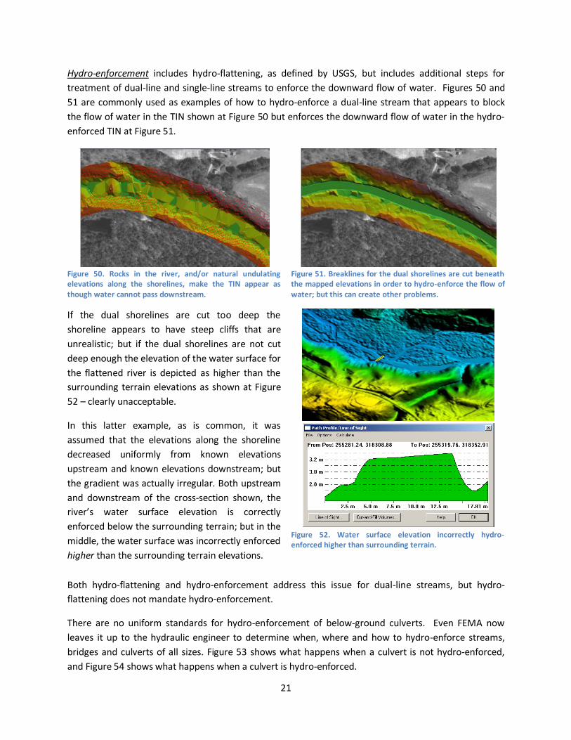
If the dual shorelines are cut too deep the
shoreline appears to have steep cliffs that are
unrealistic; but if the dual shorelines are not cut
deep enough the elevation of the water surface for
the flattened river is depicted as higher than the
surrounding terrain elevations as shown at Figure
52 – clearly unacceptable.
In this latter example, as is common, it was
assumed that the elevations along the shoreline
decreased uniformly from known elevations
upstream and known elevations downstream; but
the gradient was actually irregular. Both upstream
and downstream of the cross-section shown, the
river’s water surface elevation is correctly
enforced below the surrounding terrain; but in the
middle, the water surface was incorrectly enforced
higher than the surrounding terrain elevations.
Figure 52. Water surface elevation incorrectly hydro-enforced higher than surrounding terrain.
Both hydro-flattening and hydro-enforcement address this issue for dual-line streams, but hydro-
flattening does not mandate hydro-enforcement.
There are no uniform standards for hydro-enforcement of below-ground culverts. Even FEMA now
leaves it up to the hydraulic engineer to determine when, where and how to hydro-enforce streams,
bridges and culverts of all sizes. Figure 53 shows what happens when a culvert is not hydro-enforced,
and Figure 54 shows what happens when a culvert is hydro-enforced.
22
Figure 53. This shows what happens when the culvert is not hydro-enforced. The water flows in the ditch beside the road until it overflows the road at its shallowest elevation where the purple line crosses the road.
Figure 54. This shows the same culvert as in Figures 48 & 49, but now “cut” to hydro-enforce the flow of water through this culvert. The darkest red shows the deepest part of the “puddle” and most likely location for the culvert entrance.
Puddles are one or more elevation posts totally surrounded by higher elevations. Figures 53 and 54
show puddles with red being the deepest part of the puddle. The puddles in these examples are suitable
for hydro-enforcement, i.e., being “cut” and drained by culverts that are inferred but not absolutely
known; a “cut” is shown in Figure 54 with the purple connector line that crosses the road. Figure 28 (see
FAQ #5) shows dry puddles that should not normally be drained; it is ideal when drainage features can
be mapped when they are dry. Limestone sinks and dry swimming pools are other types of puddles that
should not normally be drained by hydro-enforcement.
FAQ #12: What are hillshades?
Hillshades have replaced contour lines as the best way to visualize 3-D topographic surfaces. Viewing
angles and sun angles can be varied to maximize visual interpretability of the terrain, as shown in
Figures 55 and 56. They normally use a color elevation ramp, but some hillshades are black and white.
Figure 55. Hillshade with 45°sun angle and 45° azimuth.
Figure 56. Hillshade with 70° sun angle and 70° azimuth.
Figure 57 shows how the B/W hillshade supplements the orthophoto in Figure 58.
23
Figure 57. Hillshades in black and white are also effective in visualization of the 3D topographic surface.
Figure 58. This color orthophoto does not reveal the topographic characteristics clearly visible in the prior figure.
FAQ #13: What are elevation derivatives?
Derived from TINs, slope and aspect are the two
most common elevation derivatives, used in many
computer models.
Figure 59 shows a simple hillshade of ridge lines
and surrounding hills.
Figure 60 shows a slope map where red areas are
the steepest and green areas are the flattest.
Figure 61 shows an aspect map of the same area
where the hottest colors are facing the sun and
the coolest colors are facing away from the sun.
Figure 59. Hillshade of ridge and hills.
Figure 60. Color-coded slope map of ridge and hills.
Figure 61. Color-coded aspect map of ridge and hills
24
As demonstrated in Figures 62 and 63, curvature is
another elevation derivative, commonly used in
applications that determine the soil wetness index.
Slope, aspect and curvature, all elevation
derivatives, are the leading parameters used in
definition of soils classifications by the Natural
Resources Conservation Service (NRCS). These
elevation derivatives are relevant also to the
hydrologic and hydraulic modeling community and
forestry, agriculture and construction industries
where slope and surface drainage are important.
Figure 62. Curvature types.
Figure 63. Plan form curvature (left); profile curvature (center); tangential curvature (right) generated from ESRI software.
FAQ #14: How frequently does elevation data need to be updated?
If you think that topographic surfaces do not change with time, these examples will demonstrate
otherwise.
Factors that Affect Hydraulic Analyses by FEMA. Volume 1, Flood Studies and Mapping, of FEMA’s
“Guidelines and Specifications for Flood Hazard Mapping Partners” explains FEMA’s procedures for
performing Mapping Needs Assessment to evaluate whether the flood hazard data and other data
shown on a Flood Insurance Rate Map (FIRM) are adequate. If the data on the FIRM are not adequate,
the community will identify the specific data elements that need to be updated, e.g., flood hazard data
for specific flooding sources, or base map information. The Mapping Needs Assessment forms the basis
for selecting and prioritizing Flood Map Projects to be initiated. In assessing flood data update needs,
FEMA requires an assessment of factors that affect hydraulic analyses (e.g., new bridges or culverts, new
flood control structures, changes in stream morphology); factors that affect still water and wave height
analyses for coastal flooding sources.
Changes in stream morphology can be critical. Any significant change in the stream channel or floodplain
geometry, particularly regarding the placement of fill, can affect the 1-percent-annual-chance floodplain
and the associated regulatory floodway. Another consideration is any change in the stream location,
25
either through natural processes (e.g., stream migration, erosion, or deposition) or through manmade
changes (e.g., channelization, stream widening, stream straightening, or dredging). Additionally, any
significant change in the vegetation or structural encroachments in the floodplain may affect a stream’s
hydraulic characteristics.
In the section entitled Minimum Standards for Community-Supplied Data, which includes elevation data
and digital orthophotos, the Currency paragraph states: “The data must have been created or reviewed
for update needs within the last 7 years.” This document was interpreted by the National Research
Council (NRC) to mean that “FEMA floodplain mapping standards require elevation data preferably
measured during the last seven years.” In two reports entitled “Elevation Data for Floodplain Mapping”
(NRC, 2007) and “Mapping the Zone: Improving Flood Map Accuracy” (NRC, 2009), the NRC strongly
recommended that FEMA collaborate with other user agencies to improve both the accuracy and
currency of elevation data used for flood hazard mapping; and FEMA has taken positive steps to
implement these NRC recommendations.
Subsidence Monitoring. Digital elevation data are used
to monitor land subsidence, the loss of surface
elevation due to removal of subsurface support.
Subsidence occurs in nearly every state in the U.S.
Subsidence is one of the most diverse forms of ground
failure, ranging from small or local collapses to broad
regional lowering of the earth’s surface. The major
causes of subsidence include: (1) dewatering of peat or
organic soils, (2) dissolution in limestone aquifers, (3)
first-time wetting of moisture deficient low density
soils (known as hydro-compaction), (4) the natural
compaction of soil, liquefaction, and crustal
deformation, and (5) subterranean mining and
withdrawal of fluids (petroleum, geothermal, and
ground water).
Figure 64 demonstrates the magnitude of the problem
in California. The sign near the top of the electric pole
shows the position of the land surface in 1925; the sign
in the middle of the pole shows the elevation in 1955;
and the sign on the ground shows the elevation of the
ground in 1977 when this photo was taken. Subsidence
has continued to the present time, and the valley has
subsided for miles in all directions.
During a five year period of drought, the California Department of Water Resources estimated the
state’s aquifers were being over-drafted at the rate of 10 million acre-feet per year. Unfortunately, the
results of over-drafting of aquifers has led to many problems caused by land subsidence, including:
Figure 64. Fifty years of subsidence in California’s San Joaquin Valley. Image courtesy of National Geodetic Survey (NGS).
26
Changes in elevation and gradient of stream channels, drains, and other water transporting
Failure of well casings from forces generated by compaction of fine-grained materials in aquifer
systems
In some coastal areas, subsidence has resulted in tidal encroachment onto lowlands
The National Research Council (NRC, 1991) conservatively estimated the annual subsidence costs due to
increased flooding and structural damage to be in excess of $125 million. These estimates do not
include loss of property value due to condemnation, and they do not consider increased farm operating
costs (re-grading of land, replacement of pipelines, replacement of damaged wells) in subsiding areas.
The NRC estimates annual subsidence costs may be about $400 million nationally, including over $180
million per year for the San Joaquin Valley, California, over $30 million per year for Santa Clara County,
California, over $30 million per year for the Houston-Galveston, Texas area, $30 million per year for New
Orleans, Louisiana, and $10 million per year for the State of Florida. The Louisiana coast line is
undergoing constant coastal change, and it is subsiding at an alarming rate ― as much as 1.5” per year is
some areas. Combined with the predicted sea level rise of 1” every 30 months, millions of people now
living in south Louisiana will see this land area and population living at and below sea level by the end of
the current century. The frequency with which LiDAR data needs to be reacquired for monitoring of
subsidence is directly proportional to the annual rate of subsidence.
Analysis of Sea Level Rise. Nearly every coastal State has requirements to predict the future impacts of
sea level rise, and credible predictions require accurate and current elevation data updated frequently.
There is currently no “rule of thumb” to indicate the frequency of topographic/bathymetric data
updates.
Sea level rise is a significant issue that threatens coastal environments and communities. According to a
report of the Environmental Protection Agency, this rise could be as high as one meter during the next
century. When the White House asked the EPA for statistics on the number of buildings to be impacted
by the predicted sea level rise, EPA attempted to use DEMs from the NED, but found them to be
unacceptable. The EPA lacked the DEMs accurate and current enough to perform this modeling effort.
Without the appropriate elevation data, it is difficult to gather a good understanding of sea level rise
impacts. This leads to problems for coastal zone managers and engineers needing to formulate
strategies to mitigate the effects of a rise in sea level. The availability of accurate elevation data can help
in understanding the possible effects of sea level rise on coastal morphology (erosion and deposition)
and ecosystem habitats that have limited vertical and horizontal positions in the coastal environment, as
shown at Figure 65.
27
Figure 65. A seamless topographic/bathymetric elevation model utilized to simulate sea level rise scenarios. The inset illustrates an approximate one meter sea level rise based on the topo/bathy DEM. Image courtesy of NOAA.
Researchers at NOAA are trying to understand the effects of sea level rise in coastal states, such as
North Carolina. One of the first steps to understanding this process is to construct an accurate DEM. In
the case of North Carolina, a seamless topo/bathy DEM was constructed utilizing the most accurate and
current elevation data available. The DEM utilized FEMA LiDAR data for topographic information and
NOAA hydrographic soundings for bathymetric information to produce a continuous bathy/topo DEM
relative to NAVD 88. Since this DEM was constructed from varying elevation data sets, these various
data sets needed to be referenced to a common vertical datum using NOAA’s VDatum tool.
To assess the impacts of sea level rise, simulations can be developed by combining a finite element
hydrodynamic model with the consistent, continuous elevation dataset. The scenarios can simulate
tidal response, synoptic wind events, and hurricane storm surge propagation in combination with sea
level rise. Accurate prediction of inundation patterns can be accomplished by merging the high
resolution, continuous bathymetric/topographic data with an accurate wetting/drying algorithm.
Shoreline migration can then be dynamically computed from the algorithm’s output as a function of sea
level rise, and coupled to characterize the effects of sea level rise on coastal ecosystems. The availability
of accurate and current high resolution bathymetric and topographic datasets holds an enormous
possibility for helping understand the impact of sea level rise to the coastal environment.
As vital input to this study, NOAA will be asked to provide their estimates of when existing elevation
data are too obsolete to be used for credible assessments of the status and impacts of sea level rise.
Monitoring of Post-Glacial Rebound. Post-glacial rebound is the rise of land masses that were depressed
by the huge weight of ice sheets during the last glacial period, through a process known as isostasy. The
enormous weight of this ice caused the surface of the Earth’s crust to deform and warp downward,
28
forcing the fluid mantle material to flow away from the loaded region. As glaciers now retreat, the
removal of the weight from the depressed land leads to slow and ongoing uplift or rebound of the land
and the return flow of mantle material back under the deglaciated area. Post-glacial rebound affects
vertical and horizontal crustal motion, global sea levels, gravity fields, vertical datums, the Earth’s
rotational motion, state of stress and intraplate earthquakes, and recent global warming.
With receding glaciers in Alaska for example, post-glacial rebound is measured vertically in centimeters
per year. Ground elevations are rising higher above sea level and boat docks at some traditional fishing
villages are now dry or too shallow for fishing boats. This has minimal impacts inland and largely
impacts coastal areas where periodic monitoring is required.
Management of Forests. LiDAR, IFSAR and stereo imagery can all be used to map the changing heights of
trees on America’s forests. How frequently do foresters need to monitor changing forest metrics? For
those who use LiDAR data to monitor forest health, how frequently do they need the LiDAR data to be
updated in order to periodically monitoring the changing health of American forests? We hope this
question can be answered as part of this questionnaire process. The ability to cut cross-sections
through LiDAR point cloud data is vital for many assessments of changes in forest metrics.
Soil Conservation. In 1935, during the peak of the “Dust Bowl,” steep slopes were clear cut, dust storms
were carrying soil from the nation’s midsection to Washington, D.C. and Hugh Hammond Bennett was
campaigning for Congressional action to stop erosion. Congress acted and passed the Soil Conservation
Act in 1935, creating the Soil Conservation Service, now known as the Natural Resources Conservation
Service (NRCS).
Hugh Hammond Bennett became the first Chief of the CSC, and he focused on management of slopes
for reduction of soil erosion. His seminal book, entitled “Elements of Soil Conservation,” had chapters
with the following names, largely linking soil erosion to management of slopes: (1) The Erosion Problem
in the Unites States, (2) Extent of Erosion, (3) Effects of Erosion, (4) How Erosion Takes Place, (5) Rates of
Erosion and Runoff, (6) Climate and Soil Erosion, (7) Rainfall Penetration, (8) A National Program of Soil
Conservation, (9) Planning for Conservation of Soil and Water, (10) Use of Vegetation in Soil and Water
Conservation, (11) Contouring, (12) Terracing, (13) Channels and Outlets, (14) Gully Control, (15) Control
of Erosion on Stream Banks, (16) Water Spreading, (17) Wildlife and Soil Conservation, (18) Farm Ponds
for Water Storage, (19) Stubble-Mulch Farming, (20) Farm Drainage, (21) Farm Irrigation, (22) The Place
of Trees and Shrubs in Soil and Water Conservation, and (23) Upstream Flood Control.
Two of Mr. Bennett’s quotes remain NRCS mottos to this day:
• “Every additional gallon of water that can be stored in the soil through the use of conservation
measures means one gallon less contributed to flood flows.”
• “Take care of the land and the land will take care of you.”
In order to participate in USDA farm programs, Federal law requires that all persons that produce
agriculture commodities must protect their highly erodible cropland from excessive erosion. In addition,
anyone participating in USDA farm programs must certify that they have not produced crops on
converted wetlands and did not convert a wetland. NRCS currently has numerous incentive programs
volcano metrics, urban modeling/change analysis, and wetland change analysis.
None of these are known to have established requirements for the frequency with which elevation
datasets need to be updated, but these examples should help questionnaire respondents to understand
that top reflective surfaces in Digital Surface Models (DSMs) and bare-earth Digital Terrain Models
(DTMs) change regularly by natural or manmade activities. As with digital orthophotos, elevation
datasets also need to be periodically updated so that 3D surface analyses can be accurate and up-to-
date for diverse user requirements.
FAQ #15: What is the National Elevation Dataset (NED)?
The National Elevation Dataset (NED) is the primary elevation data product produced and distributed by
the U.S. Geological Survey (USGS). Since its inception, the USGS has compiled and published topographic
information in many forms, and the NED is the latest development in this long line of products that
describe the land surface. The NED provides seamless raster elevation data of the conterminous United
States, Alaska, Hawaii, and the island territories. The NED is derived from diverse source data sets that
are processed to a specification with a consistent resolution, coordinate system, elevation units, and
horizontal and vertical datums. The NED is the logical result of the maturation of the long-standing
USGS elevation program, which for many years concentrated on production of map quadrangle-based
digital elevation models (DEM). The NED serves as the elevation layer of The National Map, and it
provides basic elevation information for earth science studies and mapping applications in the U.S.
To maintain seamlessness in its national coverage, the NED uses a raster data model cast in a geographic
coordinate system (horizontal locations referenced in decimal degrees of latitude and longitude). The
NED employs a multi-resolution structure, with national coverage at a grid spacing of 1-arc-second
(approximately 30 meters). The exception is Alaska where lower resolution source data warrant the use
of a 2-arc-second spacing. Where higher resolution source data exist, the NED also contains a layer at a
post spacing of 1/3-arc-second (approximately 10 meters). Some areas are also available at 1/9-arc-
second (approximately 3 meters) post spacing, where high-resolution data exist. The NED does not yet
include 1/27-arc-second data (approximately 1 meter) post spacing from highest resolution source data.
The NED production approach ensures that georeferencing of the layers results in properly nested and
coincident data across the three resolutions. In the context of the raster data model used for the NED,
the area represented by one elevation post in the 1-arc-second layer is represented by nine elevation
posts in the 1/3-arc-second layer, and by 81 elevation posts in the 1/9-arc-second layer (Figure 70).
Where all three resolution layers can be produced, each layer is constructed independently from the
same high-resolution source data using an aggregation method appropriate to the grid spacing being
produced. USGS will consider 1/27-arc-second resolution (~1 meter) if justified by user requirements.
31
An interactive map server on
the NED home page
(http://ned.usgs.gov/) allows a
user to display the NED data
source index, which indicates
the date of the most recent
update, the resolution of the
source data, and the production
method of the source data for
specific areas. The user can also
query the spatially referenced
metadata to examine additional
information about each file-
based DEM used to assemble
the NED. The NED Web site
also contains documentation on
the NED assembly process,
accuracy, metadata, standards,
data distribution, and release notes. Figure 71 shows the home page for the NED.
FAQ #16: What is the Center for LiDAR Information Coordination and Knowledge (CLICK)?
USGS’ Center for LIDAR Information Coordination and Knowledge (CLICK) is another forum for
information exchange and topographic data discovery that benefits the NED. CLICK is a virtual Web-
based center with the goal of providing a clearinghouse for LiDAR information and point cloud data.
Figure 70. NED nested multi-resolution raster elevation layers. The area represented by one elevation post (or cell) in the 1-arc-second layer is represented by nine elevation posts in the 1/3-arc-second layer and by 81 elevation posts in the 1/9-arc-second layer.
Figure 71. National Elevation Dataset (NED) home page
32
The CLICK Web site at
http://lidar.cr.usgs.gov provides
a bulletin board with numerous
topics related to LiDAR data for
discussion among the
community, including topics on
bare earth data and the National
Digital Elevation Program
(NDEP). The site also includes a
tool for viewing the coverage of
available data and downloading
point cloud data, in addition to
an extensive list of LiDAR-related
Web sites and references. Data
acquired for distribution through
the CLICK are also used as a
source of high-resolution bare
earth elevation data to enhance
the coverage of the NED 1/9-arc-
second layer. In addition,
through the CLICK, users have access to the full-return point cloud form of LiDAR data that is included in
the NED as bare earth gridded elevation data. The CLICK home page is shown at Figure 72.
FAQ #17: What are Elevation Derivatives for National Applications (EDNA)?
Elevation data are critically
important for many hydrologic
studies, and these studies are
one of the main uses of the NED
and associated derived products.
The USGS data set known as the
Elevation Derivatives for
National Applications (EDNA), at
http://edna.usgs.gov, is based
on the 1-arc-second NED and
offers a multi-layered database
that was developed specifically
for large-area hydrologic
modeling applications, including
flow direction, flow
accumulation, streamlines,
catchments, slope, and aspect.
The EDNA home page is shown at Figure 73.
Figure 72. Center for LiDAR Information Coordination and Knowledge (CLICK) home page
Figure 73. Elevation Derivatives for National Applications (EDNA) home page