Appendix A Linear Programming and Duality This appendix outlines linear programming and its duality relations. Readers are referred to text books such as Gass (1985) 1 , Charnes and Cooper (1961) 2 , Mangasarian (1969) 3 and Tone (1978) 4 for details. More advanced treatments may be found in Dantzig (1963) 5 , Spivey and Thrall (1970) 6 and Nering and Tucker (1993). 7 Most of the discussions in this appendix are based on Tone (1978). A.1 LINEAR PROGRAMMING AND OPTIMAL SOLUTIONS The following problem, which minimizes a linear functional subject to a system of linear equations in nonnegative variables, is called a linear programming problem: where and are given, and is the vector of variable to be determined optimally to minimize the scalar in the objective, c is a row vector and b a column vector. (A.3) is called a nonnegativity constraint. Also, we assume that and A nonnegative vector of variables that satisfies the constraints of (P) is called a feasible solution to the linear programming problem. A feasible solution that minimizes the objective function is called an optimal solution. A.2 BASIS AND BASIC SOLUTIONS We call a nonsingular submatrix of A a basis of A when it has the following properties: (1) it is of full rank and (2) it spans the space of solutions. We partition A into B and R and write symbolically:
Transcript
Appendix ALinear Programming and Duality
This appendix outlines linear programming and its duality relations. Readersare referred to text books such as Gass (1985)1, Charnes and Cooper (1961)2,Mangasarian (1969)3 and Tone (1978)4 for details. More advanced treatmentsmay be found in Dantzig (1963)5, Spivey and Thrall (1970)6 and Nering andTucker (1993).7 Most of the discussions in this appendix are based on Tone(1978).
A.1 LINEAR PROGRAMMING AND OPTIMAL SOLUTIONS
The following problem, which minimizes a linear functional subject to a systemof linear equations in nonnegative variables, is called a linear programmingproblem:
where and are given, and is the vector ofvariable to be determined optimally to minimize the scalar in the objective, cis a row vector and b a column vector. (A.3) is called a nonnegativity constraint.Also, we assume that and
A nonnegative vector of variables that satisfies the constraints of (P) iscalled a feasible solution to the linear programming problem. A feasible solutionthat minimizes the objective function is called an optimal solution.
A.2 BASIS AND BASIC SOLUTIONS
We call a nonsingular submatrix of A a basis of A when it has thefollowing properties: (1) it is of full rank and (2) it spans the space of solutions.We partition A into B and R and write symbolically:
282 DATA ENVELOPMENT ANALYSIS
where R is an matrix. The variable is similarly divided intoand is called basic and nonbasic. (A.2) can be expressed in
terms of this partition as follows:
By multiplying the above equation by we have:
Thus, the basic variable is expressed in terms of the nonbasic vectorBy substituting this expression into the objective function, we have:
Now, we define a simplex multiplier and simplex criterionby
where and are row vectors. The following vectors are called the basicsolution corresponding to the basis B:
Obviously, the basic solution is feasible to (A.2).
A.3 OPTIMAL BASIC SOLUTIONS
We call a basis B optimal if it satisfies:
Theorem A.1 The basic solution corresponding to an optimal basis is theoptimal solution of linear programming (P).
Proof. It is easy to see that is a feasible solution to(P). Furthermore,
Hence, by considering we find that attains its minimum when
The simplex method for linear programming starts from a basis, reducesthe objective function monotonically by changing bases and finally attains anoptimal basis.
APPENDIX A: LINEAR PROGRAMMING AND DUALITY 283
A.4 DUAL PROBLEM
Given the linear programming (P) (called the primal problem), there corre-sponds the following dual problem with the row vector of variables
Theorem A.2 For each primal feasible solution and each dual feasible so-lution
That is, the objective function value of the dual problem never exceeds that ofthe primal problem.
Proof. By multiplying (A.2) from the left by we have
By multiplying (A.16) from the right by and noting we have:
Comparing (A.18) and (A.19),
Corollary A.2 If a primal feasible and a dual feasible satisfy
then is optimal for the primal and is optimal for its dual.
Theorem A.3 (Duality Theorem) (i) In a primal-dual pair of linear pro-grammings, if either the primal or the dual problem has an optimal solution,then the other does also, and the two optimal objective values are equal.(ii) If either the primal or the dual problem has an unbounded solution, thenthe other has no feasible solution. (iii) If either problem has no solution thenthe other problem either has no solution or its solution is unbounded.
Proof, (i) Suppose that the primal problem has an optimal solution. Thenthere exists an optimal basis B and as in (A.13). Thus,
However, multiplying (A.8) on the right by B,
284 DATA ENVELOPMENT ANALYSIS
Hence,
Consequently,
This shows that the simplex multiplier for an optimal basis to the primal isfeasible for the dual problem. Furthermore, it can be shown that is optimalto the dual problem as follows: The basic solution forthe primal basis B has the objective value while has thedual objective value Hence, by Corollary A.1, is optimal for thedual problem. Conversely, it can be demonstrated that if the dual problem hasan optimal solution, then the primal problem does also and the two objectivevalues are equal, by transforming the dual to the primal form and by observingits dual. (See Gass, Linear Programming, pp. 158-162, for details).
(ii) (a) If the objective function value of the primal problem is unboundedbelow and the dual problem has a feasible solution, then by Theorem A.2, itholds:
Thus, we have a contradiction. Hence, the dual has no feasible solution.(b) On the other hand, if the objective function value of the dual problem
is unbounded upward, it can be shown by similar reasoning that the primalproblem is not feasible.
(iii) To demonstrate (iii), it is sufficient to show the following example inwhich both primal and dual problems have no solution.
where and are scalar variables.
A.5 SYMMETRIC DUAL PROBLEM
The following two LPs, (P1) and (D1), are mutually dual.
APPENDIX A: LINEAR PROGRAMMING AND DUALITY 285
The reason is that, by introducing a nonnegative slack (P1) can berewritten as (P1') below and its dual turns out to be equivalent to (D1) .
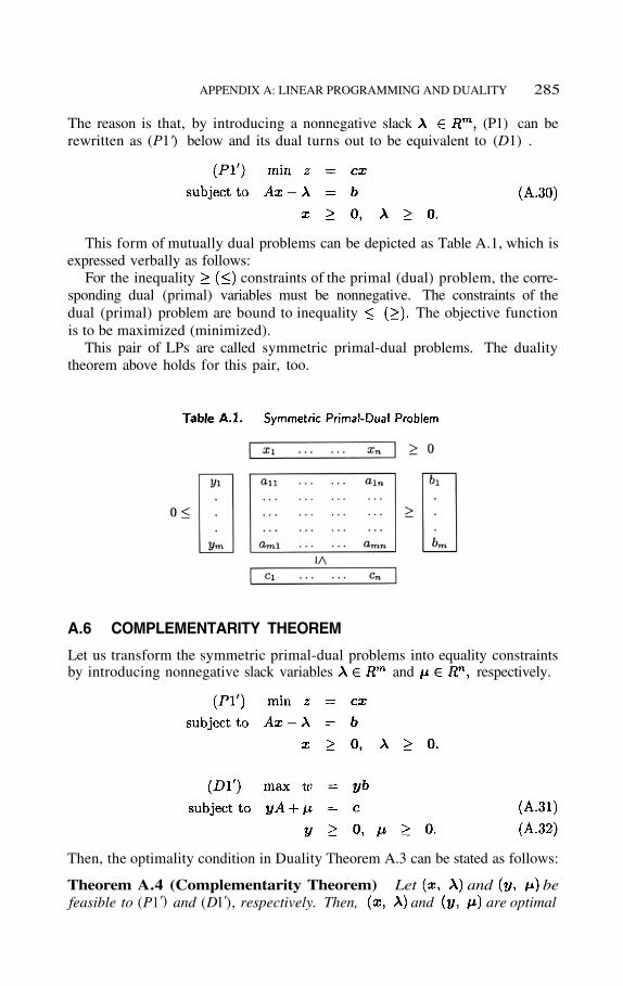
This form of mutually dual problems can be depicted as Table A.1, which isexpressed verbally as follows:
For the inequality constraints of the primal (dual) problem, the corre-sponding dual (primal) variables must be nonnegative. The constraints of thedual (primal) problem are bound to inequality The objective functionis to be maximized (minimized).
This pair of LPs are called symmetric primal-dual problems. The dualitytheorem above holds for this pair, too.
A.6 COMPLEMENTARITY THEOREM
Let us transform the symmetric primal-dual problems into equality constraintsby introducing nonnegative slack variables and respectively.
Then, the optimality condition in Duality Theorem A.3 can be stated as follows:
Theorem A.4 (Complementarity Theorem) Let and befeasible to (P1') and (Dl'), respectively. Then, and are optimal
286 DATA ENVELOPMENT ANALYSIS
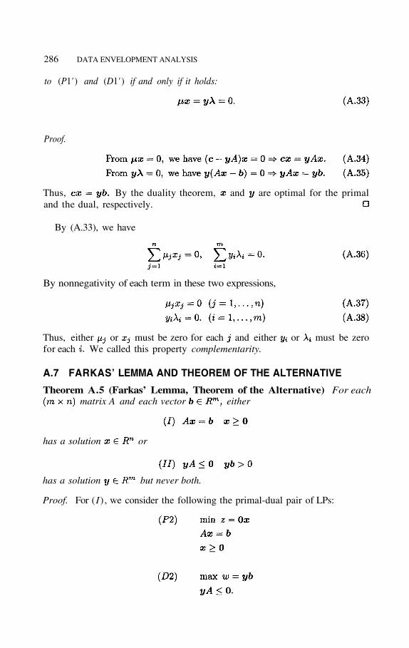
to (P1' ) and (D1' ) if and only if it holds:
Proof.
Thus, By the duality theorem, and are optimal for the primaland the dual, respectively.
By (A.33), we have
By nonnegativity of each term in these two expressions,
Thus, either or must be zero for each and either or must be zerofor each We called this property complementarity.
A.7 FARKAS’ LEMMA AND THEOREM OF THE ALTERNATIVE
Theorem A.5 (Farkas’ Lemma, Theorem of the Alternative) For eachmatrix A and each vector either
has a solution or
has a solution but never both.
Proof. For (I) , we consider the following the primal-dual pair of LPs:
APPENDIX A: LINEAR PROGRAMMING AND DUALITY 287
If (I) has a feasible solution, then it is optimal for (P2) and hence, by theduality theorem, the optimal objective value of (D2) is 0. Therefore, (II) hasno solution.
On the other hand, (D2) has a feasible solution and is not infeasible.Hence, if (P2) is infeasible, (D2) is unbounded upward. Thus, (II) has asolution.
A.8 STRONG THEOREM OF COMPLEMENTARITY
Theorem A.6 For each skew-symmetric matrix theinequality
has a solution such that
Proof. Let be the unit vector and the system be.
If has a solution then we have:
and hence
If has no solution, then by Farkas’ lemma the following system has asolution
This solution satisfies:
and hence
Since, for each either or exists, we can define a vectorby summing over Then satisfies:
Let a primal-dual pair of LPs with the coefficientand be (P1') and (D1') in Section A.6. Suppose they have optimal
288 DATA ENVELOPMENT ANALYSIS
solutions for the primal and for the dual, respectively. Then, bythe complementarity condition in Theorem A.4, we have:
However, a stronger theorem holds:
Theorem A.7 (Strong Theorem of Complementarity) The primal-dualpair of LPs (P1') and (D1 ') have optimal solutions such that, in the comple-mentarity condition (A.41) and (A.42), if one member of the pair is 0, thenthe other is positive.
Proof. Observe the system:
We define a matrix K and a vector by:
Then, by Theorem A.6, the system
has a solution
This results in the following inequalities:
We have two cases for(i) If we define and by
such that
APPENDIX A: LINEAR PROGRAMMING AND DUALITY 289
Then, is a feasible solution of (P1') and is a feasible solutionof (D1'). Furthermore, Hence, these solutions are optimal for theprimal-dual pair LPs. In this case, (A.43) and (A.44) result in
Thus, strong complementarity holds as asserted in the theorem.(ii) If it cannot occur that both (P1') and (D1') have feasible solutions.The reason is: if they have feasible solutions and then
Hence, we have:
This contradicts (A.45) in the case Thus, the case cannot occur.
A.9 LINEAR PROGRAMMING AND DUALITY IN GENERAL FORM
As a more general LP, we consider the case when there are both nonnegativevariables and sign-free variables and both inequality andequality constraints are to be satisfied as follows:
where andThe corresponding dual problem is expressed as follows, with variablesand
It can be easily demonstrated that the two problems are mutually primal-dualand the duality theorem holds between them. Table A.2 depicts the generalform of the duality relation of Linear Progrmming.
290 DATA ENVELOPMENT ANALYSIS
Now, we introduce slack variables and (DP)and rewrite them as (LP´) and (DP´) below:
We then have the following complementarity theorem:
Corollary A.3 (Complementarity Theorem in General Form)Let and be feasible to (LP') and (DP'), respectively.Then, they are optimal to (LP') and (DP'), if and only if the relation belowholds.
Also, there exist optimal solutions that satisfy the following strong complemen-tarity.
APPENDIX A: LINEAR PROGRAMMING AND DUALITY 291
Corollary A.4 (Strong Theorem of Complementarity) In the optimal so-lutions to the primal-dual pair LPs, (LP') and (DP'), there exist ones suchthat, in the complementarity condition (A.56), if one of the pair is 0, then theother is positive.
Notes
l.
2.
3.
4.
5.
6.
7.
S.I. Gass (1985) Linear Programming, 5th ed., McGraw-Hill.
A. Charnes and W.W. Cooper (1961) Management Models and Industrial Applicationsof Linear Programming, (Volume 1 & 2), John Wiley & Sons.
K. Tone (1978) Mathematical Programming, (in Japanese) Asakura, Tokyo.
G.B. Dantzig (1963) Linear Programming and Extensions (Princeton: Princeton Univer-sity Press).
W.A. Spivey and R.M. Thrall (1970) Linear Optimization (New York: Holt, Rinehartand Winston).
E.D. Nering and A.W. Tucker (1993) Linear Programming and Related Problems (NewYork: Academic Press).
292 DATA ENVELOPMENT ANALYSIS
Appendix BIntroduction to DEA-Solver
This is an introduction and manual for the attached DEA-Solver. There are twoversions of DEA-Solver, the “Learning Version” (called DEA-Solver-LV, inthe attached CD) and the “Professional Version” (called DEA-Solver-PRO:visit the DEA-Solver website at: http://www.saitech-inc.com/ for furtherinformation). This manual serves both versions.
B.1 PLATFORM
The platform for this software is Microsoft Excel 97/2000 (a trademark ofMicrosoft Corporation).
B.2 INSTALLATION OF DEA-SOLVER
The accompanying installer will install DEA-Solver and sample problems inthe attached CD to the hard disk (C:) of your PC. Just follow the instructionon the screen. The folder in the hard disk is “C:\DEA-Solver” which includesthe code DEA-Solver.xls and another folder “Samples.” It is recommended thatyou will create the shortcut to DEA-Solver.xls on the display so as to minimizestart-up time. If you want to install “DEA-Solver” to other drive or to otherfolder (not to “C:\DEA-Solver”), just copy it to the disk or to the folder youdesignate. For the “Professional Version” an installer will automatically install“DEA-Solver-PRO.”
B.3 NOTATION OF DEA MODELS
DEA-Solver applies the following notation for describing DEA models.
where I or O corresponds to “Input”- or “Output”-orientation and C or Vto “Constant” or “Variable” returns to scale. For example, “AR-I-C” meansthe Input oriented Assurance Region model under Constant returns-to-scaleassumption. In some cases, “I or 0” and/or “C or V” are omitted. For example,“CCR-I” indicates the Input oriented CCR model which is naturally underconstant returns-to-scale. “Bilateral” and “FDH” have no extensions. Theabbreviated model names correspond to the following models,
1.
2.
3.
4.
5.
CCR = Charnes-Cooper-Rhodes model (Chapters 2, 3)
BCC = Banker-Charnes-Cooper model (Chapters 4, 5)
IRS = Increasing Returns-to-Scale model (Chapter 5)
DRS = Decreasing Returns-to-Scale model (Chapter 5)
GRS = Generalized Returns-to-Scale model (Chapter 5)
<Model Name> - <I or O> - <C or V>
APPENDIX B: DEA-SOLVER 293
6.
7.
8.
9.
10.
11.
12.
13.
14.
15.
16.
17.
18.
AR = Assurance Region model (Chapter 6)
NCN = Uncontrollable (non-discretionary) variable model (Chapter 7)
BND = Bounded variable model (Chapter 7)
CAT = Categorical variable model (Chapter 7)
SYS = Different Systems model (Chapter 7)
SBM = Slacks-Based Measure model (Chapter 4)
Cost = Cost efficiency model (Chapter 8)
Revenue = Revenue efficiency model (Chapter 8)
Profit = Profit efficiency model (Chapter 8)
Ratio = Ratio efficiency model (Chapter 8)
Bilateral = Bilateral comparison model (Chapter 7)
FDH = Free Disposal Hull model (Chapter 4)
Window = Window Analysis (Chapter 9)
B.4 INCLUDED DEA MODELS
The “Learning Version” includes the following 7 models and can solve problemswith up to 50 DMUs;
CCR-I, CCR-O
BCC-I, BCC-O
AR-I-C
NCN-I-C and
Cost-C.
The “Professional Version” includes all 46 models and can deal with large-scaleproblems within the capacity of Excel worksheet. Added to the “LearningVersion” are;
IRS-I, IRS-O
DRS-I, DRS-O
GRS-I, GRS-O
AR-I-V, AR-O-C, AR-O-V
NCN-I-V, NCN-O-C, NCN-O-V
BND-I-C, BND-I-V, BND-O-C, BND-O-V
294 DATA ENVELOPMENT ANALYSIS
CAT-I-C, CAT-I-V, CAT-O-C, CAT-O-V
SYS-I-C, SYS-I-V, SYS-O-C, SYS-O-V
SBM-I-C, SBM-I-V, SBM-O-C, SBM-O-V
Cost-V
Revenue-C, Revenue-V
Profit-C, Profit-V
Ratio-C, Ratio-V
Bilateral
FDH and
Window-I-C, Window-I-V.
B.5 PREPARATION OF THE DATA FILE
The data file should be prepared in an Excel Workbook prior to execution ofDEA-Solver. The formats are as follows:
B.5.1 The CCR, BCC, IRS, DRS, GRS, SBM and FDH Models
Figure B.1 shows an example of data file for these models.
1. The first row (Row 1)The first row (Row 1) contains Names of Problem and Input/Output Items,i.e.,Cell A1 = Problem NameCell Bl, Cl, . . .= Names of I/O items.The heading (I) or (O), showing them as being input or output should headthe names of I/O items. The items without an (I) or (O) heading will notbe considered as inputs and outputs. The ordering of (I) and (O) items isarbitrary.
2.
3.
4.
The second row and afterThe second row contains the name of the first DMU and I/O values for thecorresponding I/O items. This continues up to the last DMU.The scope of data domainA data set should be bordered by at least one blank column at right and atleast one blank row at bottom. This is a necessity for knowing the scope ofthe data domain. The data set should start from the top-left cell (A1).Data sheet nameA preferable sheet name is “DAT” (not “Sheet 1”). Never use names “Score”,“Rank”, “Projection”, “Weight”, “WeightedData”, “Slack”, “RTS”, “Win-dow”, “Graphl” and “Graph2” for data sheet. These are reserved for thissoftware.
APPENDIX B: DEA-SOLVER 295
The sample problem “Hospital(CCR)” in Figure B.1 has 12 DMUs withtwo inputs “(I)Doctor” and “(I)Nurse” and two outputs “(O)Outpatient” and“(O)Inpatient”. The data set is bordered by one blank column (F) and by oneblank row (14). The GRS model has the constraint Thevalues of and must be supplied through the Message-Box onthe display by request. Defaults are L = 0.8 and U = 1.2.
As noted in 1. above, items without an (I) or (O) heading will not be consid-ered as inputs or outputs. So, if you delete “(I)” from “(I)Nurse” to “Nurse,”then “Nurse” will not be accounted for this efficiency evaluation. Thus you canadd (delete) items freely to (from) inputs and outputs without changing yourdata set.
B.5.2 The AR Model
Figure B.2 exhibits an example of data for the AR (Assurance Region) model.This problem has the same inputs and outputs as in Figure B.1. The constraintsfor the assurance region are described in rows 15 and 16 after “one blankrow” at 14. This blank row is necessary for separating the data set and theassurance region constraints. These rows read as follows: the ratio of weights“(I)Doctor” vs. “(I)Nurse” is not less than 1 and not greater than 5 and thatfor “(O)Outpatient” vs. “(O)Inpatient” is not greater than 0.2 and not lessthan 0.5. Let the weights for Doctor and Nurse be and respectively.Then the first constraint implies
Similarly, the second constraint means that the weights (for Outpatient)and (for Inpatient) satisfies the relationship
296 DATA ENVELOPMENT ANALYSIS
Notice that the weights constraint can be applied within inputs or within out-puts and cannot be applied between inputs and outputs.
B.5.3 The NCN Model
The uncontrollable (non-discretionary) model has basically the same data for-mat as the CCR model. However, the uncontrollable inputs or outputs musthave the headings (IN) or (ON), respectively. Figure B.3 exhibits the casewhere ‘Doctor’ is an uncontrollable (i.e., “non-discretionary” or “exogenouslyfixed”) input and ‘Inpatient’ is an uncontrollable output.
APPENDIX B: DEA-SOLVER 297
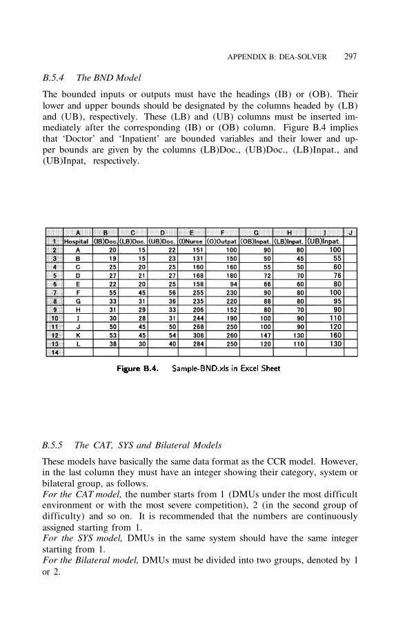
B.5.4 The BND Model
The bounded inputs or outputs must have the headings (IB) or (OB). Theirlower and upper bounds should be designated by the columns headed by (LB)and (UB), respectively. These (LB) and (UB) columns must be inserted im-mediately after the corresponding (IB) or (OB) column. Figure B.4 impliesthat ‘Doctor’ and ‘Inpatient’ are bounded variables and their lower and up-per bounds are given by the columns (LB)Doc., (UB)Doc., (LB)Inpat., and(UB)Inpat, respectively.
B.5.5 The CAT, SYS and Bilateral Models
These models have basically the same data format as the CCR model. However,in the last column they must have an integer showing their category, system orbilateral group, as follows.For the CAT model, the number starts from 1 (DMUs under the most difficultenvironment or with the most severe competition), 2 (in the second group ofdifficulty) and so on. It is recommended that the numbers are continuouslyassigned starting from 1.For the SYS model, DMUs in the same system should have the same integerstarting from 1.For the Bilateral model, DMUs must be divided into two groups, denoted by 1or 2.
298 DATA ENVELOPMENT ANALYSIS
Figure B.5 exhibits a sample data format for the CAT model.
B.5.6 The Cost Model
The unit cost columns must have the heading (C) followed by the input name.The ordering of columns is arbitrary. If an input has no cost column, its costis regarded as zero. Figure B.6 is a sample.
APPENDIX B: DEA-SOLVER 299
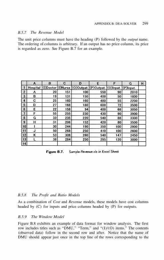
B.5.7 The Revenue Model
The unit price columns must have the heading (P) followed by the output name.The ordering of columns is arbitrary. If an output has no price column, its priceis regarded as zero. See Figure B.7 for an example.
B.5.8 The Profit and Ratio Models
As a combination of Cost and Revenue models, these models have cost columnsheaded by (C) for inputs and price columns headed by (P) for outputs.
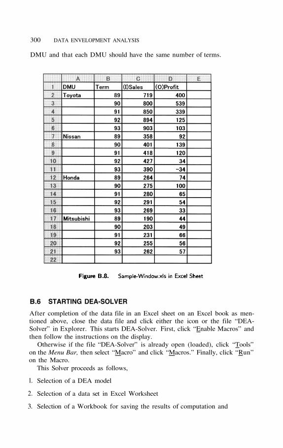
B.5.9 The Window Model
Figure B.8 exhibits an example of data format for window analysis. The firstrow includes titles such as “DMU,” “Term,” and “(I)/(O) items.” The contents(observed data) follow in the second row and after. Notice that the name ofDMU should appear just once in the top line of the rows corresponding to the
300 DATA ENVELOPMENT ANALYSIS
DMU and that each DMU should have the same number of terms.
B.6 STARTING DEA-SOLVER
After completion of the data file in an Excel sheet on an Excel book as men-tioned above, close the data file and click either the icon or the file “DEA-Solver” in Explorer. This starts DEA-Solver. First, click “Enable Macros” andthen follow the instructions on the display.
Otherwise if the file “DEA-Solver” is already open (loaded), click “Tools”on the Menu Bar, then select “Macro” and click “Macros.” Finally, click “Run”on the Macro.
This Solver proceeds as follows,
1.
2.
3.
Selection of a DEA model
Selection of a data set in Excel Worksheet
Selection of a Workbook for saving the results of computation and
APPENDIX B: DEA-SOLVER 301
4. DEA computation
B.7 RESULTS
The results of computation are stored in the selected Excel workbook. Thefollowing worksheets contain the results, although some models lack some ofthem.
1.
2.
Worksheet “Summary”This worksheet shows statistics on data and a summary report of resultsobtained.
Worksheet “Score”This worksheet contains the DEA-score, reference set, for each DMUin the reference set and ranking in input and in the descending order ofefficiency scores. A part of a sample Worksheet “Score” is displayed inFigure B.9, where it is shown that DMUs A, B and D are efficient (Score=l)and DMU C is inefficient (Score=0.882708) with the reference set composedof and and so on.
In the “Professional Version,” the ranking of DMUs in the descending orderof efficiency scores will be listed in the worksheet “Rank”.
3.
4.
Worksheet “Projection”This worksheet contains projections of each DMU onto the efficient frontierby the chosen model.
Worksheet “Weight”Optimal weights and for inputs and outputs are exhibited in this
302 DATA ENVELOPMENT ANALYSIS
worksheet. corresponds to the constraints and toIn the BCC model where holds, stands for
the value of the dual variable for this constraint.
5.
6.
7.
Worksheet “WeightedData”This worksheet shows the optimal weighted I/O values, andfor each (for
Worksheet “Slack”This worksheet contains the input excesses and output shortfalls foreach DMU.
Worksheet “RTS”In case of the BCC, AR-I-V and AR-O-V models, the returns-to-scale char-acteristics are recorded in this worksheet. For inefficient DMUs, returns-to-scale characteristics are those of the (input- or output-oriented) projectedDMUs on the frontier.
8.
9.
Graphsheet “Graph1”The bar chart of the DEA scores is exhibited in this graphsheet. This graphcan be redesigned using the Graph functions of Excel.
Graphsheet “Graph2”The bar chart of the DEA scores in the ascending order is exhibited in thisgraphsheet. A sample of Graph2 is exhibited in Figure B.10.
10. Worksheets “WindowThese sheets are only for Window models and ranges from 1 to L (thelength of time periods in the data). The contents are similar to Table 9.8
APPENDIX B: DEA-SOLVER 303
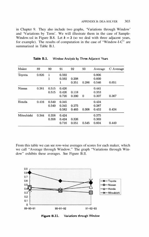
in Chapter 9. They also include two graphs, ‘Variations through Window’and ‘Variations by Term’. We will illustrate them in the case of Sample-Window.xsl in Figure B.8. Let (so we deal with three adjacent years,for example). The results of computation in the case of “Window-I-C” aresummarized in Table B.1.
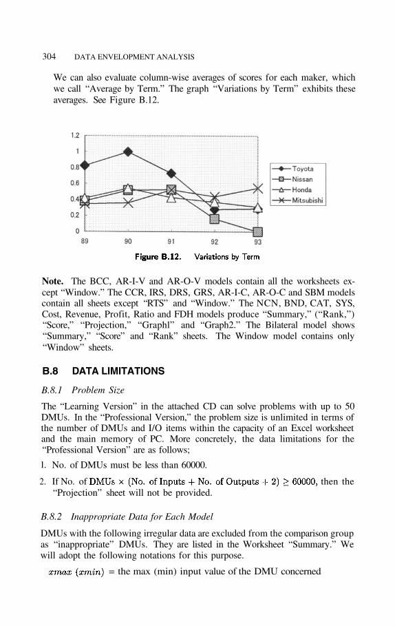
From this table we can see row-wise averages of scores for each maker, whichwe call “Average through Window.” The graph “Variations through Win-dow” exhibits these averages. See Figure B.ll.
304 DATA ENVELOPMENT ANALYSIS
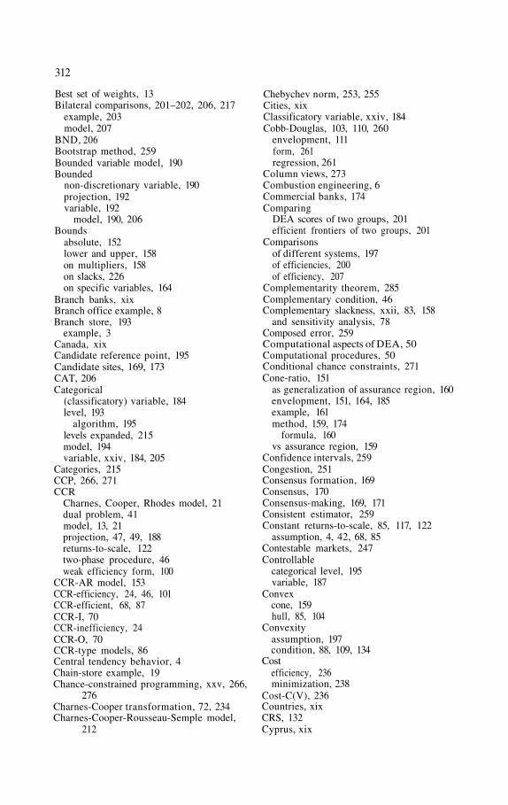
We can also evaluate column-wise averages of scores for each maker, whichwe call “Average by Term.” The graph “Variations by Term” exhibits theseaverages. See Figure B.12.
Note. The BCC, AR-I-V and AR-O-V models contain all the worksheets ex-cept “Window.” The CCR, IRS, DRS, GRS, AR-I-C, AR-O-C and SBM modelscontain all sheets except “RTS” and “Window.” The NCN, BND, CAT, SYS,Cost, Revenue, Profit, Ratio and FDH models produce “Summary,” (“Rank,”)“Score,” “Projection,” “Graphl” and “Graph2.” The Bilateral model shows“Summary,” “Score” and “Rank” sheets. The Window model contains only“Window” sheets.
B.8 DATA LIMITATIONS
B.8.1 Problem Size
The “Learning Version” in the attached CD can solve problems with up to 50DMUs. In the “Professional Version,” the problem size is unlimited in terms ofthe number of DMUs and I/O items within the capacity of an Excel worksheetand the main memory of PC. More concretely, the data limitations for the“Professional Version” are as follows;
1.
2.
No. of DMUs must be less than 60000.
If No. of then the“Projection” sheet will not be provided.
B.8.2 Inappropriate Data for Each Model
DMUs with the following irregular data are excluded from the comparison groupas “inappropriate” DMUs. They are listed in the Worksheet “Summary.” Wewill adopt the following notations for this purpose.
= the max (min) input value of the DMU concerned
APPENDIX B: DEA-SOLVER 305
= the max (min) output value of the DMU concerned
= the max (min) unit cost of the DMU concerned
= the max (min) unit price of the DMU concerned
1. For the CCR, BCC-I, IRS, DRS, GRS, CAT and SYS models, a DMUwith no positive value in inputs, i.e., will be excluded fromcomputation. Zero or minus values are permitted if there is at least onepositive value in the inputs of the DMU concerned.
For the BCC-O model, DMUs with no positive value in outputs, i.e.,will be excluded from computation.
2. For the AR model, i.e., AR-I-C, AR-I-V, AR-O-C and AR-O- V, DMUs with or will be excluded from the comparison
group.
3.
4.
5.
For the FDH model, DMUs with no positive input value, i.e., ora negative input value, i.e., will be excluded from computation.
For the Cost model, DMUs with or are excluded. DMUs with the current input will also
be excluded.
For the Revenue, Profit and Ratio models, DMUs with no positive inputvalue, i.e., no positive output value, i.e., or witha negative output value, i.e., will be excluded from computa-tion. Furthermore, in the Revenue model, DMUs with or
will be excluded from the comparison group. In the Profitmodel DMUs with or will be excluded. Finally,in the Ratio model, DMUs with ,or will be excluded.
6. For the NCN and BND models, negative input and output values are auto-matically set to zero by the program. DMUs with in the control-lable (discretionary) input variables will be excluded from the comparisongroup as “inappropriate” DMUs. In the BND model, the lower bound andthe upper bound must enclose the given (observed) value, otherwise thesevalues will be adjusted to the given value.
7. For the Window-I-C and Window-I-V models, no restriction exists for outputdata, i.e., positive, zero or negative values for outputs are permitted. How-ever, DMUs with will be characterized as being zero efficiency.This is for purpose of completing the score matrix. So, care is needed forinterpreting the results in this case.
8. For the SBM model, nonpositive inputs or outputs are replaced by a smallpositive value.
306 DATA ENVELOPMENT ANALYSIS
9. For the Bilateral model, we cannot compare two groups if some inputs arezero for one group while the other group has all positive values for thecorresponding input item.
B.9 SAMPLE PROBLEMS AND RESULTS
(1) The “Learning Version” includes the following sample problems and resultsfor reference:
Sample-CCR-I.xls
Sample-CCR-O.xls
Sample-BCC-I.xls
Sample-BCC-O.xls
Sample-AR-I-C.xls
Sample-NCN-I-C.xls
Sample-Cost-C.xls
(2) The “Professional Version” includes sample problems for all models. Visitthe Website at: http://www.saitech-inc.com/.In this version, several strategies for accelerating DEA computation for large-scale problems are employed as developed in K. Tone (1999) “Toward Efficientand Stable Computation for Large-scale Data Envelopment Analysis,” (Re-search Reports, National Graduate Institute for Policy Studies).
APPENDIX C: BIBLIOGRAPHY 307
Appendix CBibliography
Comprehensive bibliography of 1500 DEA references is available in the attachedCD-ROM.
theorem, 24Units invariant, 6, 24, 61, 97, 111, 228Universities, xix
public vs. private, 112University of Massachusetts–Amherst, xxiUniversity of Warwick, xxiUnstable point, 255USAREC, 272Variable returns-to-scale, 85Variable weights, 13–14
vs. fixed weights, 12Vector of multipliers, 51Virtual input, 21, 23, 33Virtual output, 21, 23, 33Visual Basic, xxiiWales, xixWarwick, xxi