192

APPENDIX A

SENSOR RESPONSE TIME TESTING THEORY

193

APPENDIX A

SENSOR RESPONSE TIME TESTING THEORY

This appendix contains a tutorial on sensor response time testing, including derivations

of the equations used in arriving at the results presented in the body of this thesis.

194

APPENDIX A

SENSOR RESPONSE TIME TESTING THEORY

A.1 Fundamentals of Dynamic Response

The dynamic response of a sensor or a system may be identified theoretically or

experimentally. The theoretical approach usually requires a thorough knowledge of the

design of the sensor, its construction details, the properties and geometries of the sensor's

internal material as well as a knowledge of the properties of the medium surrounding the

sensor. Since these properties are not known thoroughly, or may change under process

operating or aging conditions, the theoretical approach alone can only provide

approximate results. A remedy is to combine the theory with experiments that empirically

determine the dynamic response.

Theory is used to determine the expected behavior of the sensor in terms of an

equation called the “model,” which relates the input and the output of the system. The

system is then given an experimental input signal, and its output is measured and matched

with the model. That is, the coefficients of the model are changed iteratively until the

model matches the data within a predetermined convergence criterion. This process,

performed on a digital computer, is referred to as "fitting". Once the fitting process is

successfully completed, the coefficients of the model are identified and used to determine

the response time of the sensor. However, if the sensor can be represented with a first-

order model, fitting is not necessary because the response time can be determined directly

from the output of the sensor.

The model for a sensor or a system may be expressed in terms of either a time

domain or a frequency domain equation. The time domain model is usually a specific

relationship that gives the transient output of the system for a given input signal such as a

195

step or a ramp signal. The frequency domain model is often represented as a general

relationship called the “transfer function,” which includes the input and the output. If the

transfer function is known, the system response can be obtained for any input. As such,

the transfer function is often used in analyzing system dynamics.[A-1]

A.2 Step and Ramp Response of a First-Order System

Consider a thermocouple whose sensing section is assumed to be made of a

homogeneous material represented by the mass "m" and specific heat capacity "c", as

shown in Figure A1. The response of this system when it is suddenly exposed to a

medium with temperature (Tf) may be derived theoretically using the energy balance

equation that describes the system. Assuming that the thermal conductivity of the

thermocouple material is infinite, we can write:

( )f

dTmc hA T T

dt (A.1)

where:

h = heat transfer coefficient

A = affected surface area

T = response of the system as a function of time, t.

Equation A.1 may be solved in the frequency domain by applying a Laplace

transformation to both sides of the equation. This will allow us to express the solution in

terms of a transfer function (G) of the following equation (A.2), which relates the Laplace

transform of the output, T(s), to the Laplace transform of the input, Tf (s):

( )( )

( )f

T sG s

T s (A.2)

The Laplace transformation of Equation A.1 is:

196

Time

Se

ns

or

Ou

tpu

t

Tf

T0

Figure A.1 Step Response of a First-Order Thermal System

197

( ) (0) ( ) ( )fsT s T p T s T s (A.3)

where p = hA/mc, and s is the Laplace transform variable. Now, we can write Equation A.2

as follows, assuming that T(0) = 0:

( )( )

( )f

T s pG s

T s s p

(A.4)

In equation A.4, p is referred to as the pole of the transfer function. The reciprocal of p is

expressed in the unit of time and is called the time constant (τ) of the first-order system.

Equation A.4 can be used to derive the response of the system to any input such as a step, a

ramp, or a sinusoidal input. Proceeding to derive the step response, we substitute the

Laplace transform of a step signal in Equation A.4 to arrive at the following expression (the

Laplace transform of a step signal is “a/s”):

1 1( )

( )

paT s a

s s p s s p

(A.5)

where a is the step amplitude. The inverse Laplace transform of Equation A.5 will yield

the step response of the system, as follows:

( ) (1 )t

O t a e

(A.6)

where = 1/p. At τ = t; the step response becomes O(t) = 0.632a, and at t=, the step

response becomes O(t)=a. Thus, if we now perform an experiment in which the output of

the system is measured for a step change in input, then the resulting data can be used to

obtain the time constant (τ) directly as shown in Figure A.2. That is, the time constant of

198

63.2% of a

a

TIME

OU

TP

UT

FINAL

VALUE

Figure A.2 Determination of Time Constant from Step Response of a First-Order

System

199

the first-order system can be identified directly from the step response data by

determining the time required for the system output to reach 63.2 percent of its final

value.

The ramp response is obtained by substituting the Laplace transform of a ramp signal r/

for Tf (s) in Equation A.3:

2( )

( )

rpT s

s s p

(A.7)

where rp is a constant that we denote as k. An inverse Laplace transform of this equation

results in the ramp response (see Figure A.3):

/( ) [ ]tkO t t e

p

(A.8)

Note that when t >> the exponential term will be negligible and we can write:

( ) ( )O t k t (A.9)

That is, the asymptotic response of the system which is delayed with respect to the input

by a value that is equal to the time constant ( ) from the step response.

For a sinusoidal input, the response time is expressed in terms of the reciprocal of the

corner frequency of the frequency response plot (i.e., the break frequency of the Gain

portion of the Bode plot). If the corner frequency is denoted by the letter ω, we will show

in Equation A.10 that (1/ ) is equal to the time constant (τ) for a first-order system

(Figure A-4). Substituting jω for s in Equation A.4 and writing τ for (1/ )p , we obtain:

200

= RAMP TIME

DELAY

Input

Output

TIME

OU

TP

UT

Figure A.3 Ramp Response

b

1

FrequencyBreakb

Gain

(d

B)

Frequency (rad/s)b

MISC027-10

Figure A.4 Frequency Response of a First-Order System and Calculation of

Response Time from Break Frequency

201

1( )

1G j

j

(A.10)

where ω is the frequency in radians per second and 1- = j . The magnitude of G(jω) is:

1

2

2 2

1

1G

(A.11)

The corner frequency is the frequency at which | G | = 0.707. Substituting this in

Equation A.11 and solving for τ, we obtain 1

.

A.3 Step and Ramp Responses of Higher-Order Systems

Although some systems, such as the simple thermal system discussed in section

A.2, can be approximated with a first-order model, the transient behavior of most systems

is generally written in terms of higher-order models that are represented by a transfer

function of the following form:

1 2

( ) 1( )

( ) ( )( ) ( )f n

T sG s

T s s p s p s p

(A.12)

where p1 , p2 , . . ., pn are called the poles of the system transfer function. The reciprocal

of these poles are denoted as τ1 , τ2 , . . ., τn , which are called modal time constants. The

following derivations (Equations A.13 through A.23) show that the overall time constant

of a system is obtained by combining its modal time constants.

The response of a higher-order system to a step change in input is derived by

substituting ( ) 1/fT s s in Equation A.12 and performing an inverse Laplace transform.

This yields:

202

1

2

1 2

1 2 1 1 2 1

1 2

2 2 1 2

( )( ) ( )1( ) 1

( )( ) ( ) ( ) ( )

( )( ) ( )

( ) ( )

p tn

n n

p tn

n

p p pT t e

p p p p p p p p

p p pe

p p p p p

(A.13)

From this, we can write:

1 2

1 2

1( )

( )( ) ( )n

n

Tp p p

(A.14)

Thus:

11 2

1 1 2 1

1

( )1

( ) 1 1 1 1 1

t

n

n

T te

T

(A.15)

21 2

2 2 1 2

1

1 1 1 1 1

t

n

n

e

Now we proceed to determine the expressions that yield the overall response time (τ) of

the system in terms of its modal time constants 1 2 3( , , , ). For typical process

sensors, we can safely assume, based on experience with their dynamic response curves,

that the values of the modal time constants rapidly decrease as we go from 1 to 2 to

n . Thus, if we let 1 be the slowest time constant (the largest in value) and evaluate the

second exponential at 1/ = 1, we obtain the following:[A-2]

203

1

2

2/

1( )te at t

______ _________________

2 0.135

3 0.050

4 0.018

5 0.007

___________________________________________

For a sensor such as an RTD, 1 2/ is typically about 5 or greater. Therefore, the

contribution of 2 is small by the time t = 1 . Since 1 has the most important effect on

, we can also assert that 2 and higher terms have a small influence when t = . Thus,

we may write:

11 2

1 1 2 1

1

( )1

( ) 1 1 1 1 1

t

n

n

T te

T

(A.16)

Now, we can set ( )

( )

T t

T = 0.632 and solve for to obtain:

1/ 32

1 1 1

0.368(1 )(1 ) (1 )ne

(A.17)

Or:

321

1 1 1

1 ln(1 ) ln(1 ) ln(1 )n

(A.18)

For ramp response, we substitute 2

k

s for Tf (s) in Equation A.12, where k is the ramp rate:

204

2

1 2

( )( )( ) ( )n

kT s

s s p s p s p

(A.19)

The sensor response may be evaluated by inverse Laplace transformation. The partial

fraction method yields:

31 2 4

2

1 2

( ) n

n

A AA A AO s

s s s p s p s p

(A.20)

The arbitrary constants Ais must be evaluated if the complete response is required.

However, we are interested only in determining the ramp time delay. Consequently, the

exponential terms are of no interest, and we can concentrate on A1 and A2. These may be

evaluated to give the following result:[A-3]

1

2 1 2 n

A k

A k

(A.21)

Therefore:

1 2( ) ( )nO k (A.22)

In this case, we obtain:

1 2 nRamp Time Delay (A.23)

Equations A.18 and A.23 show that (a) the time constant of a first-order system is equal

to the ramp time delay of the system and that (b) as the order of the system increases,

205

the time constant and the ramp time delay slowly depart from one another, with the

ramp delay time greater than the time constant.

206

REFERENCES

A-1 Kerlin, T.W., “Frequency Response Testing in Nuclear Reactors,” Academic

Press, New York, (1974)

A-2 U.S. Nuclear Regulatory Commission “Safety Evaluation Report Review of

Resistance Temperature Detector Time Response Characteristics.” NUREG-

0809, Washington, DC (1981).

A-3 Electric Power Research Institute Report NP-267, “Sensor Response Time

Verification,” EPRI, Palo Alto, California (October 1976).

207

APPENDIX B

PRESSURE SENSORS AND SENSING LINE DYNAMICS

208

APPENDIX B

PRESSURE SENSORS AND SENSING LINE DYNAMICS

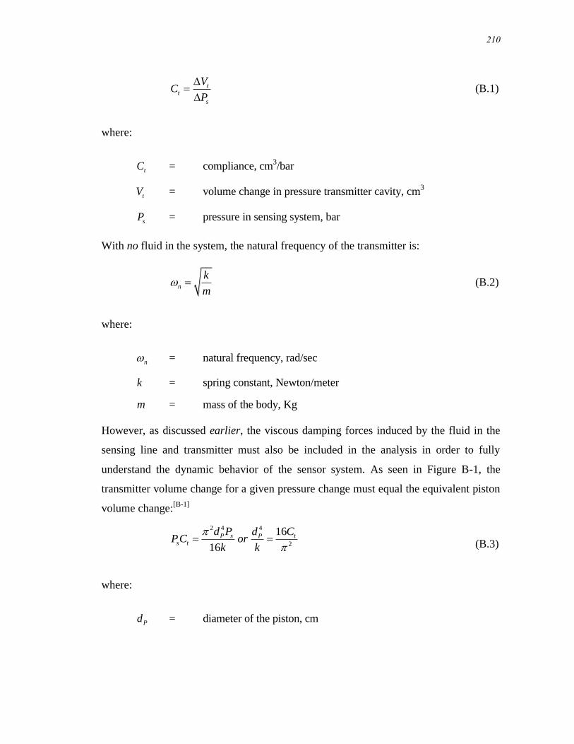
This appendix contains the derivations of the formulas used in the body of this thesis to

arrive at results that simulated the effects of length, blockages, and voids on the response

time of a pressure sensing system (pressure transmitter and sensing line). In applying

these formulas, the natural frequency and damping ratio of the system had to be

calculated based on the physical properties (e.g., dimension, compliance, fluid density,

bulk modulus, etc.) of the pressure sensing system. The resulting values were then used

in the solutions to a second-order, underdamped linear differential equation to arrive at

time domain and frequency domain results in terms of tables of numbers and PSD plots.

209

APPENDIX B

PRESSURE SENSORS AND SENSING LINE DYNAMICS

Figure B.1 illustrates a mechanical model of a pressure transmitter and its sensing line,

which together constitute a pressure sensing system. The pressure transmitter is

represented by a spring-mass viscous assembly that emulates a viscously damped single-

degree-of-freedom system. As the process pressure Pp changes, the subsequent pressure

surge is transmitted through the sensing line and results in a volume change (Vt) in the

pressure transmitter cavity. To describe the relationship between the volume change in

the transmitter and the pressure required to induce this volume change, the term

compliance Ct is used. The compliance is defined as the change in transmitter volume

that results from a change in pressure.

Process

Sensing

Line

Pressure

Transmitter

Fixed

Boundary

PRESS014-05

Figure B.1 Pressure Sensing System Model

210

tt

s

VC

P

(B.1)

where:

tC = compliance, cm3/bar

tV = volume change in pressure transmitter cavity, cm3

sP = pressure in sensing system, bar

With no fluid in the system, the natural frequency of the transmitter is:

n

k

m (B.2)

where:

n = natural frequency, rad/sec

k = spring constant, Newton/meter

m = mass of the body, Kg

However, as discussed earlier, the viscous damping forces induced by the fluid in the

sensing line and transmitter must also be included in the analysis in order to fully

understand the dynamic behavior of the sensor system. As seen in Figure B-1, the

transmitter volume change for a given pressure change must equal the equivalent piston

volume change:[B-1]

2 4 4

2

16

16

P s tPs t

d P CdPC or

k k

(B.3)

where:

Pd = diameter of the piston, cm

211

As the process pressure Pp increases or decreases, the kinetic energy of the fluid in the

sensing line will change, depending on the mass and velocity of the fluid. The mass of

the fluid is dependent on the volume of the fluid in the sensing line, and the velocity can

be calculated by assuming a square velocity profile for the fluid in the sensing line.

Based on this, the kinetic energy of the fluid can be shown to equal the following:

2 2

8

s sF

LV dKE

(B.4)

where:

FKE = kinetic energy of the fluid

ρ = Fluid density, g/cm3

L = Length of the sensing line, cm

Vs = Average velocity of fluid in the sensing line, m/s

ds = Inside diameter of the sensing line, cm

Noting that a rigid mass (representing the equivalent of a fluid mass attached to the

piston mass m) must have the same kinetic energy as the fluid, the mass can be shown

to equal:

4

24

p

e

s

LdM

d

(B.5)

where:

eM = rigid mass, g

The natural frequency of the pressure transmitting sensing line system then equals:

212

n

e

k

M m

(B.6)

For most cases Me >> m, therefore, the natural frequency equation reduces to:

n

e

k

M (B.7)

Substituting Equations B.3 and B.5 into Equation B.7 provides the new equation (B.8)

for the natural frequency of the system:

2

4

sn

t

d

LC

(B.8)

The damping ratio can also be calculated, as shown in Equation B.9. Note that the

damping force is directly related to the pressure drop in the system due to the fluid

viscosity (assuming that laminar conditions exist):

32

3tLC

ds

(B.9)

where

ζ = damping ratio

= dynamic viscosity of the fluid, Bar∙second

Equation B.9 can be further simplified by relating it to a nondimensional variable called

the Stokes number:[B-2]

2

n sn

dS

v

(B.10)

213

nS = Stokes number

v = kinematic viscosity of the fluid, Bar∙second

Substituting the equation for the natural frequency (Equation B.8) into Equation B.10

results in the Stokes number at the natural frequency of the system:

2 2

4

s sn

t

d dS

LC

(B.11)

Solving for μ yields:

2 2

4

s s

n t

d d

S LC

(B.12)

Substituting Equation B.12 into B.9 provides an equation that relates the Stokes number

to the damping ratio at the natural frequency of the system:

2

16 16

n n s

v

S d

(B.13)

To account for other factors that are usually present in a pressure sensing system, the

compliance should be modified to include: (1) the compliance of the fluid in the

transmitter, (2) the compliance of the fluid in the sensing line, and (3) the compliance

of any entrapped gas that might be present in the system.[B-2]

That is:

s t FT FS BC C C C C (B.14)

SC = compliance of the total system, cm3/bar

FTC = compliance of the fluid in the transmitter, cm3/bar

FSC = compliance of the fluid in the sensing line, cm3/bar

214

BC = compliance of any entrapped gas that might be present in the

system, cm3/bar

The remaining terms of this equation are as follows:

2

4, ,t FS b

FT FS B

b

V V VC C and C

B B P (B.15)

where:

VFS = Volume of fluid in the sensing line, cm3

Vb = Volume of gas bubble, cm3

γ = Ratio of specific heats for gas bubble

Pb = Pressure applied to gas bubble, mbar

B = Bulk modulus for the fluid, bar

2

4t t FS

s b

V V V VbCs

P B B P

(B.16)

Therefore,

2 22

2 2

4 4 '

4 4 4

t t bs FS

s b

V V BV CC B V

B P P B

(B.17)

If the total system compliance Cs is considered instead of just Ct , then substituting

Equation B.17 into Equation B.7 yields:

2

1 '4 2

FSn

p

B

VBA

LC L C

(B.18)

215

where:

A = cross-sectional area of the sensing line, cm2

For infinitely stiff pipe walls, the acoustic velocity of the fluid in the sensing line can be

approximated as follows:

BUa

(B.19)

where:

Ua = acoustic velocity of the fluid, m/s

B = bulk modulus for the fluid

Therefore, using Equation B.17, the natural frequency of the system becomes:

22

4

a FSn

bt t FS

b

U V

L VBC B V V

P

(B.20)

The equation to calculate the natural frequency and damping ratio of the pressure

sensing system enables us to describe the dynamic characteristics of the system in terms

of step and ramp responses. To do so, we use the following relationships for linear

second-order responses:

216

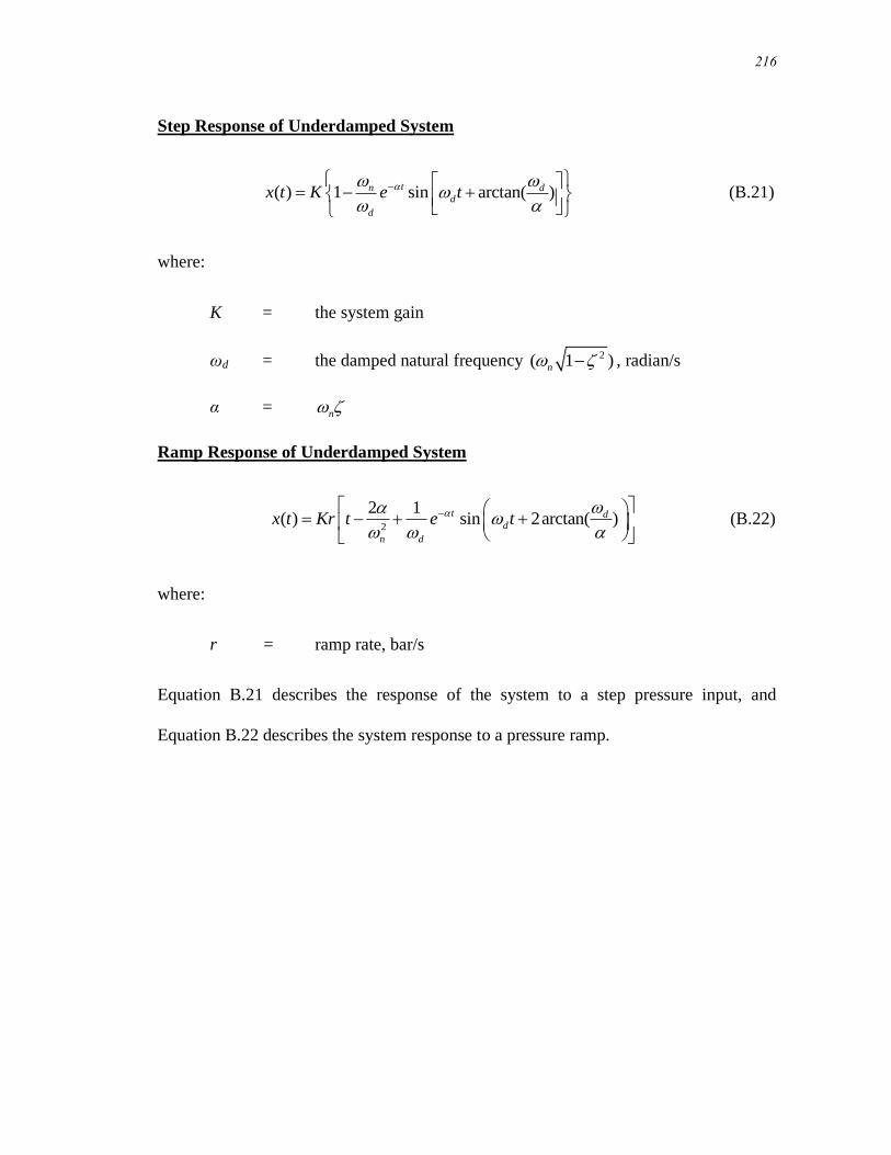
Step Response of Underdamped System

( ) 1 sin arctan( )tn dd

d

x t K e t

(B.21)

where:

K = the system gain

ωd = the damped natural frequency 2( 1 )n , radian/s

α = n

Ramp Response of Underdamped System

2

2 1( ) sin 2arctan( )t d

d

n d

x t Kr t e t

(B.22)

where:

r = ramp rate, bar/s

Equation B.21 describes the response of the system to a step pressure input, and

Equation B.22 describes the system response to a pressure ramp.

217

REFERENCES

B-1 Doebelin, Ernest O., “Measurement Systems: Application and Design,”

McGraw-Hill Book Co., Inc., 5th

Edition, 2005.

B-2 Anderson, R.C., Englund, Jr., D.R., “Liquid-Filled Transient Pressure

Measuring Systems: A Method for Determining Frequency Response,” NASA

TN D-6603 (December 1971).

218

APPENDIX C

CORRELATIONS BETWEEN RESPONSE TIME AND

PROCESS CONDITIONS

219

APPENDIX C

RTD RESPONSE TIME VERSUS PROCESS CONDITIONS

In the body of this thesis, we stated that an RTD's response time depends on the process

conditions in which the sensor is used. In this appendix, we develop correlations to

quantify process condition effects by measuring response time in the laboratory at

ambient conditions and extrapolating the results to process operating conditions. The

correlations are useful to sensor designers, manufacturers, and users who seek to

estimate the response time of a temperature sensor at process operating conditions based

on data from laboratory measurements.

C.1 Response Time versus Flow Rate

The response time of an RTD or a thermocouple consists of an internal component and

a surface component. The internal component depends predominantly on the thermal

conductivity (k) of the material inside the sensor, while the surface component depends

on the film’s heat-transfer coefficient (h). The internal component is independent of the

process conditions, with the exception of the effect of temperature on material

properties. The surface component is predominantly dependent on the process

conditions, such as flow rate, temperature, and to a lesser extent, the process pressure.

These parameters affect the film’s heat-transfer coefficient, which increases as the

process parameters such as flow rate and temperature are increased. Figure C.1

illustrates how a temperature sensor’s response time may decrease as h is increased. In

this illustration, the effect of temperature on the material properties inside the sensor is

ignored.

220

TEMP023-01

Figure C.1 Internal and Surface Components of Response Time as a Function of

Heat-Transfer Coefficient

221

To derive the correlation between the fluid flow rate and response time (τ), we recall the

following equation for the response time ( ) of a first-order thermal system:

mc

UA (C.1)

In this equation, m and c are the mass and specific heat capacity of the sensing portion,

respectively, and U and A are the overall heat transfer coefficient and the affected

surface area of the temperature sensor, respectively. Note that we used the overall heat-

transfer coefficient, U, as opposed to the film heat-transfer coefficient, h. The overall

heat transfer coefficient accounts for the heat transfer resistance both inside the sensor

and at the sensor surface. More specifically, we can write:[C-1]

int

1 1

tot surf

UAR R R

(C.2)

where:

Rtot = total heat-transfer resistance

Rint = internal heat-transfer resistance

Rsurf = surface heat-transfer resistance.

For a homogeneous cylindrical sheath, the internal and surface heat transfer resistances

may be written as follows for a single-section lumped model:

int

ln( / )

2

o ir rR

kL (C.3)

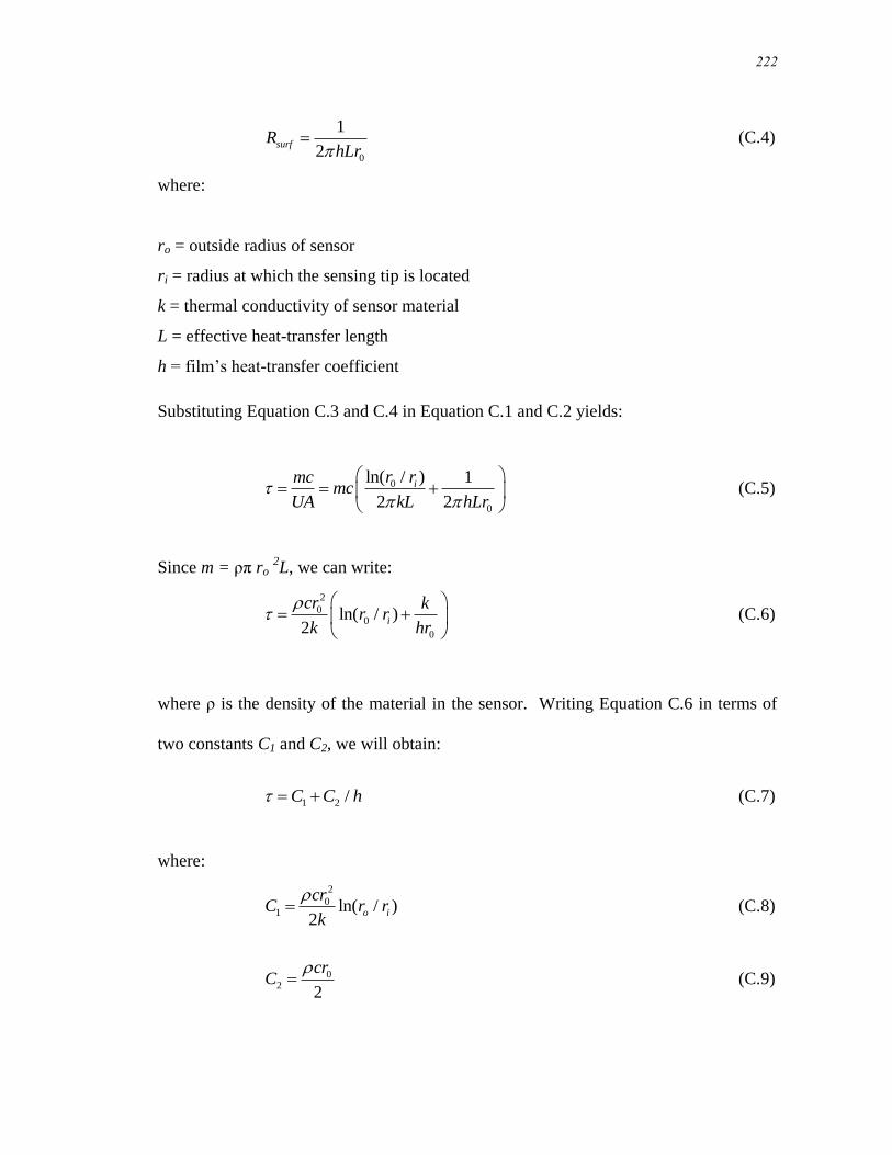
222

0

1

2surfR

hLr (C.4)

where:

ro = outside radius of sensor

ri = radius at which the sensing tip is located

k = thermal conductivity of sensor material

L = effective heat-transfer length

h = film’s heat-transfer coefficient

Substituting Equation C.3 and C.4 in Equation C.1 and C.2 yields:

0

0

ln( / ) 1

2 2

ir rmcmc

UA kL hLr

(C.5)

Since m = ρπ ro 2L, we can write:

2

00

0

ln( / )2

i

cr kr r

k hr

(C.6)

where ρ is the density of the material in the sensor. Writing Equation C.6 in terms of

two constants C1 and C2, we will obtain:

1 2 /C C h (C.7)

where:

2

01 ln( / )

2o i

crC r r

k

(C.8)

02

2

crC

(C.9)

223

We can use Equation C.7 to estimate the response time of a temperature sensor at

process operating conditions based on the response time measurements made in a

laboratory. The procedure is to make laboratory response time measurements in at least

two different heat-transfer media (with different values of h) in order to identify C1 and

C2. Once we have identified C1 and C2, we can use Equation C.7 to estimate the

temperature sensor’s response time in process media for which we can calculate the

value of h based on the type of media and its temperature, pressure, and flow

conditions.

A useful application of Equation C.7 is to estimate the response time of a temperature

sensor at a given process flow rate based on response time measurements made in a

laboratory setup. More specifically, we can derive a correlation for response time-

versus-fluid flow rate by determining the relationship between the heat-transfer

coefficient (h) in Equation C.7 and the fluid flow rate (u). We obtain the heat-transfer

coefficient by using general heat-transfer correlations that involve the Reynolds

number, Prandtl number, and Nusselt number, which have the following relationships:

Nu = f (Re, Pr) (C.10)

In Equation C.10, Nu = hD/k is the Nusselt number, Re = Duρ/μ is the Reynolds

number, and Pr = cμ/k is the Prandtl number. These heat-transfer numbers are all

dimensionless, and their parameters are defined as follows:

h = film’s heat-transfer coefficient

D = sensor’s diameter

k = thermal conductivity of process fluid

224

u = average velocity of process fluid

ρ = density of process fluid

μ = viscosity of process fluid

c = specific heat capacity of process fluid

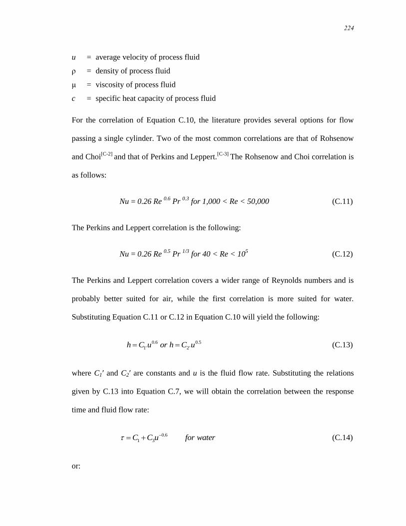
For the correlation of Equation C.10, the literature provides several options for flow

passing a single cylinder. Two of the most common correlations are that of Rohsenow

and Choi[C-2]

and that of Perkins and Leppert.[C-3]

The Rohsenow and Choi correlation is

as follows:

Nu = 0.26 Re 0.6

Pr 0.3

for 1,000 < Re < 50,000 (C.11)

The Perkins and Leppert correlation is the following:

Nu = 0.26 Re 0.5

Pr 1/3

for 40 < Re < 105 (C.12)

The Perkins and Leppert correlation covers a wider range of Reynolds numbers and is

probably better suited for air, while the first correlation is more suited for water.

Substituting Equation C.11 or C.12 in Equation C.10 will yield the following:

0.6 0.5

1' 2'h C u or h C u (C.13)

where C1′ and C2′ are constants and u is the fluid flow rate. Substituting the relations

given by C.13 into Equation C.7, we will obtain the correlation between the response

time and fluid flow rate:

0.6

1 3C C u for water (C.14)

or:

225

0.5

1 4C C u for air (C.15)

Using either of the two Equations C.14 or C.15, one can identify the two constants of

the response-versus-flow correlation for a given sensor by making measurements at two

or more flow rates in water or in other convenient media in a laboratory. Once these

constants are identified, they can be used to estimate the sensor’s response time in other

media for which the flow rate (u) is known.

C.2 Response Time versus Temperature

Unlike flow, the effect of temperature on a temperature sensor’s response time cannot

be estimated with great confidence. This is because temperature can either increase or

decrease a temperature sensor’s response time. Temperature affects both the internal

and the surface components of the response time. Its effect on the surface component is

similar to that of the flow. That is, as temperature is increased, the film’s heat-transfer

coefficient (h) generally increases and causes the surface component of response time to

decrease. However, temperature’s effect on the internal component of response time is

more subtle. High temperatures can cause the internal component of response time to

either increase or decrease depending on how temperature affects the properties and on

the geometry of the material inside the sensor. Because of differences in the thermal

coefficient of expansion of the material inside the sensor and the sheath, the insulation

material inside the sensor may become either more or less compact at higher

temperatures. Consequently, the sensor material’s thermal conductivity, and therefore

the internal response time, can either increase or decrease. Furthermore, voids such as

gaps and cracks in the sensor’s construction material can either expand or contract at

226

high temperatures. This causes the internal response time to either increase or decrease

depending on the size, orientation, and location of the void. At high temperatures, the

sheath sometimes expands so much that an air gap is created at the interface between

the sheath and the insulation material inside the sensor. In this case, the response time

can increase significantly with temperature. It is possible, however, to account for

temperature’s effect on the surface component of response time. In the following

paragraph we will use equation C.14 to demonstrate this point for a sensor in water.

Neglecting temperature’s effect on the internal component of response time, the term C1

in Equation C.14 will be unchanged. Therefore, we only need to account for

temperature’s effect on the second term of Equation C.14. For a given reference flow

rate, it can be shown that the second term of Equation C.14 is affected by temperature

as follows:[4]

13 2 3 1

2

( )( ) ( )

( )

h TC T C T

h T

(C.16)

Therefore, if we know the value of constant C3 at room temperature (approximately

21°C), we can find its value at temperature (T2) if we know h(21°C)/h(T2). Based on

Equation C.12 (Rohsenow and Choi correlation), we can write:

0.7 0.3 0.6 0.3(21 )(4.3612) ( ) ( ) ( ) ( )

( )

o

p

h CK T T T C T

h T (C.17)

From the Perkins and Leppert correlation, we have:

2/3 1/6 0.50 1.3(21 )(3.3603) ( ) ( ) ( ) ( )

( )

o

p

h CK T T T C T

h T (C.18)

227

A plot of Equations C.17 and C.18 for water is shown in Figure C.2. The data in this

figure are for a pressure of approximately 140 bars (about 2000 psi). However, since the

properties of water are not strongly dependent on pressure, the data should hold for

pressures of up to about ±30 percent of 140 bars. Note that there is a large difference

between the two curves in Figure C.2. This arises from the fact that two different heat-

transfer correlations are used.

The data in Figure C.2 can be used to identify the heat transfer ratio that is needed in

Equation C.16 to calculate C3 at a given temperature based on measurements made at

room temperature. This C3 is then used in Equation C.14 to determine the response

time-versus-flow curve of a sensor at any given temperature. Figure C.3 shows

response time-versus-flow rate results at two different temperatures for an RTD. These

results are derived from plunge tests of the RTD in room temperature water at different

flow rates. The response time results from these plunge tests were used together with

the corrections developed in this appendix and the Rohsenow and Choi correlation data

of Figure C.2 to arrive at the results presented in Figure C.3.

228

300250200150100500

0.5

0.6

0.7

0.8

0.9

1.0

1.1

From Rohsenow and Choi Correlation

From Perkins and Leppert Correlation

Water Temperature (C)

h(2

1C

)/h

(T)

TEMP012-04

Figure C.2 Correlations for Determining the Effect of Temperature on

Response Time of Temperature Sensors

229

Figure C.3 RTD Response-versus-Flow Results at Two Different Temperatures

230

REFERENCES

C-1 Kerlin, T. W., Hashemian, H. M., Petersen, K. M., “Time Response of

Temperature Sensors,” Paper C.I. 80-674, Instrument Society of America (now

ISA - The International Society of Automation), International Conference and

Exhibit, Houston, Texas (October 1980).

C-2 Rohsenow, W. M., Choi, H. Y., “Heat, Mass and Momentum Transfer,”

Prentice-Hall, Englewood Cliffs, NJ (1961).

C-3 Perkins, H. C., Leppert, G., "Forced Convection Heat Transfer from a

Uniformly Heating Cylinder," Journal of Heat Transfer, No. 84, pp. 257-263

(1962).

231

APPENDIX D

SELF-HEATING INDEX AND ITS CORRELATION

WITH RTD RESPONSE TIME

232

APPENDIX D

SELF-HEATING INDEX AND ITS CORRELATION WITH

RTD RESPONSE TIME

This appendix develops the correlation between the self-heating index (SHI) of an RTD

and its response time and presents the procedure for measuring SHI. Like the LCSR

test, self-heating measurements can be performed remotely on RTDs as installed in an

operating plant. The results are used for two purposes: (1) to calculate the self-heating

error in steady-state temperature measurement with RTDs, and (2) to trend SHI as a

way of monitoring for gross degradation of RTD response time. (The self-heating error

is an inherent phenomenon in RTDs that arises from the use of an electronic current that

must be applied to the RTD to measure its resistance.) Typically, both self-heating

measurements and LCSR tests are performed together in nuclear power plants to

provide a complete picture of the dynamic health of an RTD.

D.1 SHI Measurement

A Wheatstone bridge is used to perform a self-heating test on an RTD and to measure

its SHI. The measurement may be made in a laboratory to provide baseline data, or

while the RTD is installed in a plant to provide a trendable value with which to monitor

for response time degradation.

The following procedure is used:

1. Connect the RTD to a Wheatstone bridge (Figure D-1). The same Wheatstone

bridge arrangement that is used for the LCSR test can also be for a self-heating

test.

2. Adjust the bridge power supply to run a small current (1 to 2 mA) through the

RTD.

3. Balance the bridge and record the first self-heating data point, which consists of

the RTD resistance (R) and the bridge of the current (I). The RTD resistance is

the same as the value that is shown on the decade box when the bridge is

balanced. The current may be measured with a multimeter across one of the

fixed resistors in the bridge.

233

+

-

(When Bridge is Balanced)

Figure D-1 Wheatstone Bridge Arrangement for Self-Heating Test

234

4. Calculate the power input to the RTD using the P = I2R equation and fill the

result in a table such as Table D-1.

5. Increase the bridge current to about 10 mA, wait for steady state, balance the

bridge, record the next self-heating data point in table D-1, and calculate the new

value of power.

6. Increase the current by about 5 mA, wait for steady state, balance the bridge,

record the new values of R and I, and calculate the new value of power. Repeat

this step until the current is 40 to 60 mA depending on the amount of current that

is allowed for the RTD.

7. Plot the resistance data (R) versus power (P). This is called the self-heating

curve, which is typically a straight line for a normal RTD (Figure D-2).

8. Calculate the slope of the self-heating curve. This is referred to as the self-

heating index or SHI, and its value is expressed in terms of ohms/watt (/w).

Table D-1 Self-Heating Data for an RTD from Testing in a Nuclear Power

Plant

Resistance (ohms) Current (ma) Power (mw)

423.4 11.5 55.7

424.0 20.7 181.2

425.1 32.1 438.8

426.4 41.4 732.2

428.1 51.2 1123.1

Results

Self Heating Index: 4.4

(ohms/watt)

235

422

424

426

428

430

0 400 800 1200

Resis

tan

ce (

Oh

ms)

Power (mW)

Self-Heating Index (SHI) = 4.4 ohms/watt

Self-Heating Curve

Raw Data

Figure D-2 Self-Heating Curve of an RTD Being Tested in a Nuclear Power

Plant

236

D.2 Correlation between SHI and Response Time

The steady-state relation between temperature and I2R heating generated in an RTD is

given by:

Q UA(T ) (D.1)

where:

Q = Joule heating generated in the RTD by applying I2R heating

U = overall heat-transfer coefficient at the RTD’s sensing tip

(includes both internal and surface heat transfer)

A = heat-transfer area

T = RTD temperature

= temperature of fluid in which the RTD is installed

For constant fluid temperature, Equation D.1 may be written as follows:

Q UA T (D.2)

Therefore, the temperature rise per unit power generated in the RTD is:

1T

Q UA

(D.3)

The resistance of the RTD’s platinum element is approximately proportional to its

temperature (i.e., R T where α is the temperature coefficient of resistance).

Thus:

R Cons tant

Q UA

(D.4)

237

On the other hand, an RTD’s response time is approximately given by the following

equation, assuming that the RTD is a first-order system:

mc

UA (D.5)

where:

m = mass of the sensing tip of the sensor

c = specific heat capacity of the sensor material

If the heat capacity c remains constant, then:

Constant

UA (D.6)

Comparing equations D.6 and D.4 leads to the conclusion that τ is proportional to QΔ

RΔ

That is: R

or SHIQ

(D.7)

where R / Q is equal to SHI, and α represents proportionality. Equation D.7 shows

that a change in an RTD’s response time can be identified from a change in its SHI.

D.3 Temperature Rise in the LCSR Test

In this section, we calculate the temperature rise in an RTD for a self-heating value of

4.4 Ω /W and 40 mA of current. If the RTD is a 200-ohm sensor, at a PWR temperature

of 300oC, its resistance will be about 424 ohms. With 40 mA of current, 0.68 watts of

power will be generated in the RTD. With a self-heating index of 4.4 Ω/W, this will

cause a 3.0 ohm increase in resistance. Using a temperature coefficient of resistance of

0.8 Ω/oC for the 200 ohm RTD, this corresponds to about 3.75

oC. That is, in this RTD,

a LCSR current of 40 mA will increase the RTD temperature by 3.75oC above the

process temperature.