Appendix A Theoretical Background of Nonlinear System ...

Appendix ATheoretical Background of Nonlinear SystemStability and Control

. . . Mr. Fourier had the opinion that the main purpose ofmathematics was public utility and explanation of naturalphenomena, but a philosopher like him should have known thatthe sole purpose of science is the honor of the human spirit, andthat, as such, a matter of numbers is worth as much as a matterof the world system.

Letter from Jacobi Legendre, July 2nd, 1830

Automatic control comprises a number of theoretical tools of mathematical charac-teristics that enable to predict and apply its concepts to fulfill the objectives that aredirectly attached to it. These tools are necessary for the synthesis of control laws ona specific process and are utilized at various stages of the design. This is more so,particularly during the modeling and identification of the parameters stage as wellas during the construction of control laws and during the verification of the stabilityof the controlled system, just to mention a few. In fact, it is well-known that all con-struction techniques of control laws or observation are narrowly linked to stabilityconsiderations.

As a result, in the first part of this appendix, some definitions and basic conceptsof stability theory are recalled. The second part of the appendix is dedicated to thepresentation of some concepts and techniques of control theory.

Due to the numerous contributions in this area, in the past few years, we havefocused our interest only on points that are more directly related to our own work.

A.1 Stability of Systems

One of the tasks of the control engineer consists, very often, in the study of stability,whether for the considered system, free from any control, or for the same systemwhen it is augmented with a particular control structure. At this stage, it might beuseful or even essential to ask what stability is. How do we define it? How to con-ceptualize and formalize it? What are the criteria upon which one can conclude onthe stability of a system?

A. Choukchou-Braham et al., Analysis and Control of Underactuated MechanicalSystems, DOI 10.1007/978-3-319-02636-7,© Springer International Publishing Switzerland 2014

93

http://dx.doi.org/10.1007/978-3-319-02636-7

94 A Theoretical Background of Nonlinear System Stability and Control

A.1.1 What to Choose?

It is clear that drawing up an inventory as complete as possible of the forms ofstability that have appeared throughout the history of automatic control but alsoof mechanics would be beyond the scope of this book. There will therefore notbe included in this presentation the stability method of Krasovskii [70], comparisonmethod, singular perturbations [37], the stability of the UUB (Uniformly UltimatelyBounded) [15], the input–output stability [94], the input to state stability [71], thestability of non-autonomous systems [2], contraction analysis [34], and descriptivefunctions [70].

In addition, we will not be presenting the proofs of various results in this section.We will assume that the conditions of existence and the uniqueness of solutions forthe considered systems of differential equations are verified everywhere.

From a notation point of view, we shall denote by x(t, t0, x0) the solution attime t with initial condition x0 at time t0 or by x(t, t0, x0, u) when the system iscontrolled. In addition, for simplicity, we shall frequently use the notation x(t) oreven x, when the dependence on t0, x0 or t is evident. Similarly, we shall considerin the majority of cases, except in some cases, the initial time t0 = 0.

The class of systems considered will be those that can be put in the followingordinary differential equation (ODE) form:

x = f (x) (A.1)

where x ∈ Rn is the state vector and f : D → R

n a locally Lipschitzian functionand continuous on the subset D of Rn.

This type of systems is also called autonomous due to the absence of the temporalterm t in the function. Non-autonomous systems of the form x = f (x, t) are notconsidered in this work.

For the above equation (A.1), the point of the state space x = 0 is an equilibriumpoint if it verifies

f (0) = 0 ∀t ≥ 0 (A.2)

Note that, by a change of coordinates, one can always bring the equilibrium point tothe origin.

A.1.2 The Lyapunov Stability Theory

The Lyapunov stability theory is considered as one of the cornerstones of automaticcontrol and stability for ordinary differential equations in general. The original the-ory of Lyapunov dates back to 1892 and deals with the study of the behavior ofsolution of differential equation for different initial conditions. One of its applica-

A.1 Stability of Systems 95

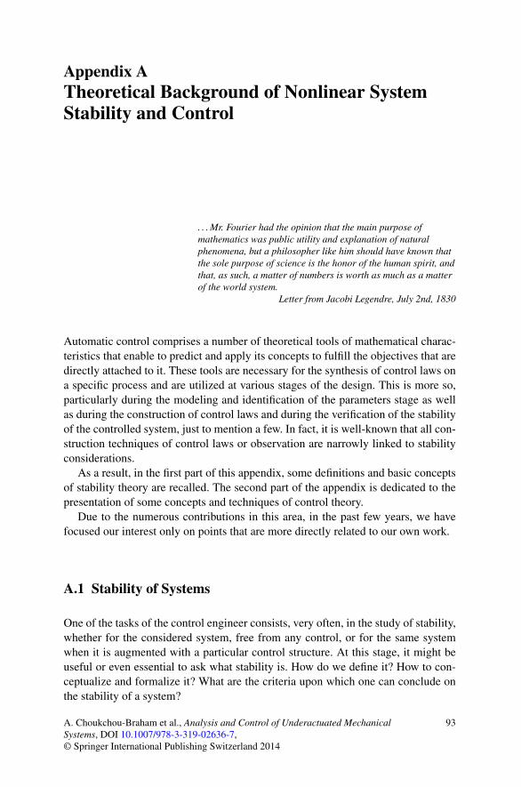
Fig. A.1 Intuitive illustrationof stability

tions that was contemplated at that time was the study of librations in astronomy.12

The emphasis is focused on the ordinary stability (i.e. stable but not asymptoticallystable), which we can represent as a robustness with respect to initial conditions,and the asymptotic stability is only addressed in a corollary manner.

The automatic control community having inverted this preference, we will beconcentrating here on the concept of asymptotic stability rather than mere stability.

Note that there are many more complete presentations of Lyapunov stability inmany articles, for example [37, 49, 55, 62, 65, 66, 70, 87], which constitute the mainreferences of this part; this list also does not claim to be exhaustive.

A.1.2.1 Stability of Equilibrium Points

Roughly speaking, we say that a system is stable if when displaced slightly from itsequilibrium position, it tends to come back to its original position. On the otherhand, it is unstable if it tends to move away from its equilibrium position (seeFig. A.1).

Mathematically speaking, this is translated into the following definitions:

Definition A.1 [37] The equilibrium point x = 0 is said to be:

• stable, if for every ε > 0, there exists η > 0 such that for every solution x(t) of(A.1) we have

∥∥x(0)

∥∥ < η ⇒ ∥

∥x(t)∥∥ < ε ∀t ≥ 0

• unstable, if it is not stable, that is, if for every ε > 0, there exists η > 0 such thatfor every solution x(t) of (A.1) we have

∥∥x(0)

∥∥ < η ⇒ ∥

∥x(t)∥∥ ≥ ε ∀t ≥ 0

• attractive, if there exists r > 0 such that for every solution x(t) of (A.1) we have∥∥x(0)

∥∥ < r ⇒ lim

t→∞x(t) = 0

The basin of attraction of the origin is defined by the set B such that

x(0) ∈ B ⇒ limt→∞x(t) = 0

1In astronomy, the librations are small oscillations of celestial bodies around their orbits.2The father of Alexander Michael Lyapunov was an astronomer.


Fig. A.2 Stability andasymptotic stability of x

• globally attractive, if for every solution x(t) of (A.1) we have

limt→∞x(t) = 0. In this case, B = R

n

• asymptotically stable, if it is stable and attractive, and globally asymptoticallystable (GAS), if it is stable and globally attractive.

• exponentially stable, if there exist r > 0, M > 0 and α > 0 such that for everysolution x(t) of (A.1) we have

∥∥x(0)

∥∥ < r ⇒ ∥

∥x(t)∥∥ ≤ M

∥∥x(0)

∥∥e−αt for all t ≥ 0

and globally exponentially stable (GES), if there exist M > 0 and α > 0 such thatfor every solution x(t) of (A.1) we have

∥∥x(t)

∥∥ ≤ M

∥∥x(0)

∥∥e−αt for all t ≥ 0

Remark A.1

1. The difference between stable and asymptotically stable is that a small perturba-tion on the initial state around a stable equilibrium point x might lead to smallsustained oscillations, whereas these oscillations are dampened in time in thecase of asymptotically stable equilibrium point, see Fig. A.2 (U1 is the ball ofcenter 0 and radius ε and U2 is the ball of center 0 and radius η [46]).

2. For a linear system, all these definitions are equivalent (except for stable andasymptotically stable). However, for a nonlinear system, stable does not implyattractive, attractive does not imply stable, asymptotically stable does not implyexponentially stable whereas exponentially stable implies asymptotically stable.

When the systems are represented by nonlinear differential equations, the verifi-cation of stability is not trivial. On the contrary, for linear systems the verificationof stability is systematic and is determined as follows.

A.1.2.2 Stability of the Origin for a Linear System

Consider the linear system

x = Ax (A.3)

where A is a square matrix of dimension n. Let λ1, . . . , λs , be the distinct eigenval-ues with algebraic multiplicity m(λi) of the matrix A.


Theorem A.1 [37]

1. If ∃j Re(λj ) > 0 or if ∃k Re(λk) = 0 and m(λk) > 1 then x = 0 is unstable.2. If ∀j Re(λj ) < 0 then x = 0 is exponentially (hence asymptotically) stable.3. If Re(λj ) < 0 and if ∃k Re(λk) = 0 and m(λk) = 1 then x = 0 is stable but not

attractive.

Unfortunately, there does not exist an equivalent theorem to that of eigenvaluesfor nonlinear systems. In some cases, one can characterize the stability of the originvia the study of the linearized system.

A.1.2.3 Linear Approximation of a System

Consider a system of the form (A.1); we denote by

A = ∂f

∂x(x)

the Jacobian matrix of f evaluated at the equilibrium point x = x. The obtained sys-tem will be of the form (A.3) and is called the linearization (or linear approximation)of the nonlinear system (A.1).

Theorem A.2 [37]

1. If x = 0 is asymptotically stable for (A.3) then x = x is asymptotically stable for(A.1).

2. If x = 0 is unstable for (A.3) then x = x is unstable for (A.1).3. If x = 0 is stable but not asymptotically stable for (A.3) then we cannot conclude

on the stability of x = x for (A.1).

Another criterion that allows to conclude on the stable behavior of the system forboth linear and nonlinear system is described next.

A.1.2.4 Lyapunov’s Direct Method

The principle of this method is a mathematical extension of the following physi-cal phenomenon: if the total energy (of positive sign) of a mechanical or electricalsystem is continuously decreasing then the system tends to reach a minimal energyconfiguration. In other words, to conclude on the stability of a system, it suffices toexamine the variations of a certain scalar function called Lyapunov function withouthaving to solve the explicit solution of the system. This is precisely the strong pointof this method since the equation of motion of x(t) does not have to be computedin order to characterize the evolution of the solution (the determination of explicitsolutions of nonlinear system is difficult and sometimes impossible).


Lyapunov Function Consider the system

x = f (x) with f (0) = 0 (A.4)

x = 0 is an equilibrium point for (A.4) and D ⊂ Rn is a domain that contains x = 0.

Let V : D → R be a function that admits continuous partial derivatives. We de-note

V (x) = ∂V (x)

∂x· f (x) =

n∑

i=1

∂V (x)

∂xi

· fi(x)

the derivative of the function V in the direction of the vector field f .

Definition A.2 The function V is a Lyapunov function for system (A.4 ) at x = 0in D, if for all x ∈ D we have

• V (x) > 0 except at x = 0 where V (0) = 0• V (x) ≤ 0.

Theorem A.3 [37]

1. If there exists a Lyapunov function for (A.4) at x = 0 in a neighborhood D of 0,then x = 0 is stable.

2. If, in addition, x �= 0 ⇒ V (x) < 0 then x = 0 is asymptotically stable.3. If, in addition, D = R

n and V (x) → ∞ when ‖x‖ → ∞ then x = 0 is GAS.

Remark A.2

1. V depends only on x, it is sometimes called the derivative of V along the system.2. This derivative is also called Lie derivative and is denoted by Lf V .3. To calculate V , we do not require the knowledge of x but of x, that is, of f (x).

Hence, for the same function V (x), V is different for different systems.4. For every solution x(t) of (A.4), we have d

dtV (x(t)) = V (x(t)), consequently

if V is negative, V decreases along the solution of (A.4) so that the trajectoriesconverge towards the minimum of V .

5. When V (x) → ∞ whenever ‖x‖ → ∞, V (x) is said to be radially unbounded.6. V (x) is often a function that represents the energy or a certain form of energy of

the system.7. From a geometric point of view, a Lyapunov function is seen as a bowl whose

minimum coincides with the equilibrium point. If this point is stable, then thevelocity vector x (or f ), tangent to every trajectory will point towards the interiorof the bowl, see Fig. A.3 [46].

LaSalle’s Invariance Principle

Definition A.3 A set G ⊆ Rn is said to be positively invariant if every solution x(t)

such that x(0) ∈ G remains in G for all t ≥ 0.


Fig. A.3 Lyapunovfunction V for vector fields f

If x is an equilibrium point then {x} is positively invariant.

Theorem A.4 ([37] (Lyapunov–LaSalle)) Let V : D → R+ be a function having

continuous partial derivatives such that there exists l for which the region Dl definedby V (x) < l is bounded V (x) ≤ 0 for all x ∈ Dl . Let R = {x ∈ Dl : V (x) = 0}and let M be the largest positively invariant set that is included in R. Then, everysolution issued from Dl tends to M when t → ∞. In particular if {0} is the onlyorbit contained in R then x = 0 is asymptotically stable and Dl is contained in itsbasin of attraction.

Theorem A.5 [37] Let V : Rn → R+ be a function having continuous partial

derivatives. Suppose that V (x) is radially unbounded and that V (x) ≤ 0 for allx ∈ R

n. Let R = {x ∈ Rn : V (x) = 0} and let M be the largest positively invariant

set that is included in R. Then, every solution tends to M when t → ∞. In particularif {0} is the only orbit contained in R then x = 0 is GAS.

Remark A.3

1. The criteria for stability and asymptotic stability presented in Theorems A.3, A.4and A.5 are easy to utilize. However, they do not give any information on howto construct the Lyapunov function. In reality, there does not exist any generalmethod for the construction of Lyapunov functions except for some particularclasses of systems (namely for the class of linear systems).

2. The theorems given previously give sufficient conditions in the sense that if for acertain Lyapunov function V , the conditions on V are not satisfied, this does notimply that the considered system is unstable (maybe with another function onecan demonstrate the stability of the system).

3. Contrary to Lyapunov functions which guarantee the stability of the equilibriumpoints, there are functions, called Chetaev functions, that guarantee the instabil-ity of the equilibrium points. Note that it is more difficult to demonstrate theinstability rather than stability (refer to [46] for more details).

In some cases, a dynamical system is represented, at a given instant of time t ≥ t0,not by a single set of continuous differential equations, but by a family of contin-uous subsystems together with a logic orchestrating the switching between thesesubsystems: this is the class of switching systems.


In this book we have employed some controllers for this class of systems. Con-sequently, in what follows, we shall present the stability criteria for these systems.We shall present the controller design for this class of system for a later stage.

A.1.3 Stability of Switching Systems

Mathematically speaking, a switching system can be described by equations of theform

x = fp(x) (A.5)

where {fp : p ∈ P} is a family of functions sufficiently regular defined from Rn to

Rn and parameterized by a set of indices P.For the system (A.5), the active subsystem at every instant of time is determined

by a sequence of switches of the form

σ = (

(t0,p0), (t1,p1), . . . , (tk,pk), . . .)

(t0 ≤ t1 ≤ · · · ≤ tk)

σ is called the switching signal and can depend either on time or on the state orboth. Such systems are said to have variable structures or are called multi-models.They represent a particularly simple class of hybrid systems [10, 81, 85].

Here, we shall assume that the origin is an equilibrium point that is commonfor the individual subsystems fp(0) = 0. We shall also assume that the switchingis done without jumps and does not occur infinitely fast so that the Zeno phe-nomenon is avoided. The reader who is interested in these properties can refer to[6, 53, 63, 64].

The class of systems often considered in the literature are those for which theindividual systems are linear

x = Apx (A.6)

Just to mention a few, we cite the following references: [11, 26, 51, 50, 52, 54, 68,75, 74, 90, 95, 96, 97]. On the other hand, there are only few works in the literaturefor the class of nonlinear switching systems [9, 12, 16, 19, 47, 53, 98, 99].

At this stage one might ask the following question: given a switching system,why do we need a theory of stability that is different from that of Lyapunov?

The main reason is that the stability of switching systems depends not only onthe different dynamics corresponding to several subsystems but also on the transitionlaw that governs the switchings. In effect, we have the case where two subsystemsare exponentially stable while the switching between the two subsystems drives thetrajectories to infinity.

In fact, it was shown in [12, 19, 47] that a necessary condition for the stability ofswitching systems subjected to an arbitrary transition law is that all the individualsubsystems should be asymptotically stable, but this condition was not sufficient.Nevertheless, it appears that when the switching between the subsystems is suffi-ciently slow (so as to allow the transition period to settle down and to allow each


subsystems to be in steady state) then it is very likely that the global system will bestable.

A.1.3.1 Common Lyapunov Function

It is clear that in the case where the family of systems (A.5) possesses a commonLyapunov function V (x) such that ∇V (x)fp(x) < 0 for all x �= 0 and all p ∈ P,then the switching system is asymptotically stable for any transition signal σ [47].Hence, a possibility for demonstrating the stability of switching systems consists infinding a common Lyapunov function for all the individual subsystems of (A.5).

However, finding a Lyapunov function for a nonlinear system, even for a singleone is not simple. If, in addition, we allow the switchings between several subsys-tems, the determination of such a function becomes much more difficult. It is alsothe reason for which a non-classical theory of stability is necessary.

A.1.3.2 Multiple Lyapunov Functions

In the case where a common Lyapunov function cannot be determined, the idea isto demonstrate the stability through several Lyapunov functions. One of the firstresults of such procedure was developed by Peleties in [58, 59], then by Liberzon[47], for the switching systems of the form (A.6).

Given N dynamical systems Σ1, . . . ,ΣN , and N pseudo Lyapunov functions(Lyapunov-like functions) V1, . . . , VN .

Definition A.4 [19] A pseudo Lyapunov function for system (A.5) is a functionVi(x) with continuous partial derivatives defined on a domain Ωi ⊂ R

n, satisfyingthe following conditions:

• Vi is positive definite: Vi(x) > 0 and Vi(0) = 0 for all x �= 0.• V is semi negative definite: for x ∈ Ωi ,

Vi(x) = ∂Vi(x)

∂xfi(x) ≤ 0 (A.7)

and Ωi is the set for which (A.7) holds true.

Theorem A.6 [19] Suppose that⋃

i Ωi = Rn. For i < j , let ti < tj be the tran-

sition instants for which σ(ti) = σ(tj ) and suppose that there exists γ > 0 suchthat

Vσ(tj )

(

x(tj+1)) − Vσ(ti )

(

x(ti+1)) ≤ −γ

∥∥x(ti+1)

∥∥2

. (A.8)

Then, the system (A.6) with fσ(t)(x) = Aσ(t)x and the transition function σ(t) isGAS.


Fig. A.4 Energy profile ofthe linear switching systemfor N = 2

The condition (A.8) is illustrated by Fig. A.4.The first generalization of this theorem to nonlinear systems is due to Branicky

[9, 10, 11, 12]

Theorem A.7 [9, 10] Given N switching systems of the form (A.5) and N pseudoLyapunov functions Vi in the region Ωi associated to each subsystem, and supposethat

⋃

i Ωi = Rn and let σ(t) be the transition sequence that takes the value i when

x(t) ∈ Ωi . If in addition,

Vi

(

x(ti,k)) ≤ Vi

(

x(ti,k−1))

(A.9)

where ti,k is the kth time where fi is active, that is, σ(t−i,k) �= σ(t+i,k) = i, then (A.5)is stable in the sense of Lyapunov.

Figure A.5 illustrates the condition (A.9) (in dotted lines) [19]. A more generalresult due to Ye [91, 92] concerns the utilization of weak Lyapunov functions forwhich condition (A.9) is replaced by

Vi

(

x(t)) ≤ h

(

Vi

(

x(tj )))

, t ∈ (tj , tj+1) (A.10)

where h : R+ → R+ is a continuous function with h(0) = 0 and tj is any transition

instant when the system i is activated.In this case, it is no longer required that the Lyapunov functions be decreasing.

It suffices that they are bounded by a function that is zero at the origin. Hence, theenergy can grow in the intervals where the same system is activated but must bedecreasing at the end of these intervals, see Fig. A.5 (solid lines).

Liberzon in [47] extends these results by giving a condition on multiple Lya-punov functions in order to demonstrate the global asymptotic stability.

Consider N subsystems of the form (A.5). When the subsystems of the family(A.5) are assumed to be asymptotically stable, then there exists a family of Lya-punov functions {Vp : p ∈ P} such that the value of Vp decreases on each intervalfor which the pth subsystem is active.


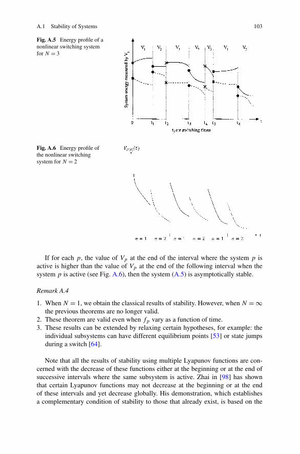
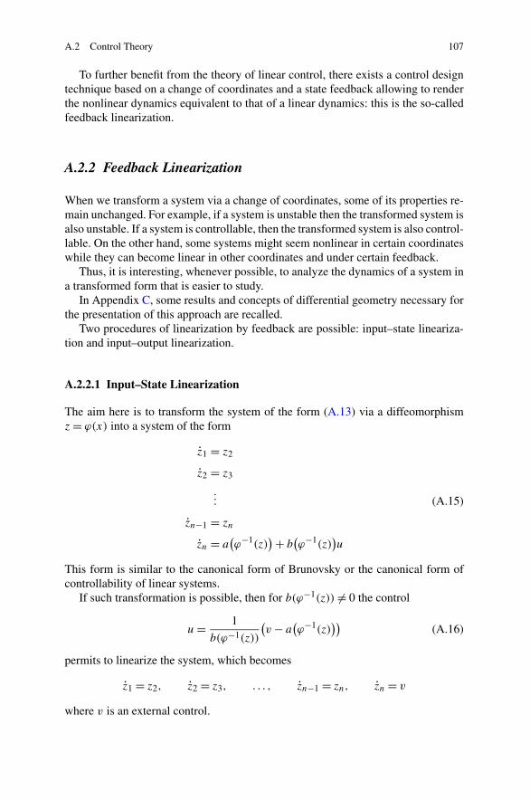
Fig. A.5 Energy profile of anonlinear switching systemfor N = 3

Fig. A.6 Energy profile ofthe nonlinear switchingsystem for N = 2

If for each p, the value of Vp at the end of the interval where the system p isactive is higher than the value of Vp at the end of the following interval when thesystem p is active (see Fig. A.6), then the system (A.5) is asymptotically stable.

Remark A.4

1. When N = 1, we obtain the classical results of stability. However, when N = ∞the previous theorems are no longer valid.

2. These theorem are valid even when fp vary as a function of time.3. These results can be extended by relaxing certain hypotheses, for example: the

individual subsystems can have different equilibrium points [53] or state jumpsduring a switch [64].

Note that all the results of stability using multiple Lyapunov functions are con-cerned with the decrease of these functions either at the beginning or at the end ofsuccessive intervals where the same subsystem is active. Zhai in [98] has shownthat certain Lyapunov functions may not decrease at the beginning or at the endof these intervals and yet decrease globally. His demonstration, which establishesa complementary condition of stability to those that already exist, is based on the


Fig. A.7 Illustration of theaverage values of Vi(x(T

ji ))

evaluation of the average value of Lyapunov functions during the intervals wherethe same subsystem is active.

Evidently, in the case where the subsystems are GAS, the result is practicallyequivalent to the previous results. However, his conditions are given with respect tothe decrease of the average Lyapunov functions on the same intervals, see Fig. A.7.

Theorem A.8 [98] Suppose that the N subsystems of (A.5), associated to N radi-ally unbounded Lyapunov functions are GAS. Define the average value of the Lya-punov functions during the activation period for each subsystem as

Vi

(

x(

Tji

)) Δ= 1

t2ji − t

2j−1i

∫ t2ji

t2j−1i

Vi

(

x(τ))

dτ(

t2j−1i ≤ T

ji ≤ t

2ji

)

(A.11)

Then, the switched system is GAS in the sense of Lyapunov if, for all i,

Vi

(

x(

Tj+1i

)) − Vi

(

x(

Tji

)) ≤ −Wi

(∥∥x

(

Tji

)∥∥)

(A.12)

holds for a positive definite continuous function Wi(x).

Additionally, this result is extended to the case when the subsystems are not sta-ble under the condition that the Lyapunov functions are bounded. In this case, if theaverage value of the Lyapunov functions decreases on the set of intervals associ-ated to a subsystem i, then the switching system (A.5) is asymptotically stable, seeFig. A.8 [98].

Remark A.5 More recently, a similar result to the above using the average valueof the derivative of the Lyapunov functions, rather than the average value of theLyapunov functions, for the stability analysis of linear switching systems has beengiven by Michel in [54].

Recall that the stability is the first step in the study of a system in terms of itsperformance evaluation. In fact, if a system is not stable (or not stable enough), itis important to proceed to the stabilization of this system before looking to satisfyother performances such as trajectory tracking, precision, control effort, perturba-tion rejection, robustness, etc.

A.2 Control Theory 105

Fig. A.8 Illustration of thedecrease of energy in thepresence of unstable systems

A.1.4 Stabilization of a System

The problem of stabilization consists in maintaining the system near an equilibriumpoint y∗. The aim is to construct stabilizing control laws such that y∗ becomes anasymptotically stable equilibrium point of the system under these control laws.

Remark A.6

1. The problem of trajectory tracking consists in maintaining the solution of thesystem along a desired trajectory yd(t), t ≥ 0. The objective here is to find acontrol law such that for every initial condition in a region D, the error betweenthe output and the desired output

e(t) = y(t) − yd(t)

tends to 0 when t → ∞. In addition, the state must remain bounded.2. Note that the stabilization problem around an equilibrium point y∗ is a special

case of the problem of trajectory tracking whereby

yd(t) = y∗, t ≥ 0

The control design techniques allowing to construct control laws for the stabiliza-tion of systems are numerous and varied. In what follows, we are going to presentthose that are most useful for the control of underactuated mechanical systems. Themain references where most of the results on this subject were borrowed from, inthe next section, are [32, 37, 41, 43, 44, 66, 67].

A.2 Control Theory

Given a physical system that we want to control and the system behavior we want toobtain, designing a control amounts to construct control laws such that the systemsubjected to these laws (the closed-loop system) presents the desired behavior.


Nonetheless, the control procedure is only possible if the system in question iscontrollable. Otherwise, the uncontrollable modes would need to be stable [13]. Formore details, please refer to Appendix D.

The synthesis of control laws for nonlinear systems is difficult in general. There-after, we propose some control design techniques for the class of nonlinear controlaffine systems of the form

x = f (x) + g(x)u, x ∈ Rn, u ∈R (A.13)

The linearizability is a property that renders the systems more easy to control.In addition, the control design techniques for linear systems are well-establishedand largely developed. We can cite some examples such as pole placement control,optimal control, and a frequency-based approach just to mention a few. For moredetails on these subjects the interested reader can refer to [2, 17, 24, 35, 42, 56, 93].This list is far from complete obviously.

Thus, it might be useful to highlight this linearizability property for nonlinearsystems too. In what follows, the most employed and well-known procedures arebriefly recalled.

A.2.1 Local Stabilization

Consider the system of the following form:

x = f (x) + g(x)u, f (0,0) = 0

In the presence of the control input u, the linear approximation around the equilib-rium point is given by

x = Ax + Bu (A.14)

where the matrices A and B are defined by

A = ∂f

∂x(0,0), B = ∂f

∂u(0,0).

The obtained form (A.14) justifies the utilization of linear control techniques men-tioned above.

Unfortunately, the resulting linearized system is typically valid only around theconsidered point so that the associated controller is valid only in a neighborhood ofthis point. This leads to a local control only. In addition, determining the linearitydomain is not obvious.

In Appendix B, the reader will find more details of the limits of linearization andthe underlying dangers of destabilization.

Hence, even though this method is simple and practical, it is necessary to proceeddifferently in order to increase the validity domain of the synthesized controllers.


To further benefit from the theory of linear control, there exists a control designtechnique based on a change of coordinates and a state feedback allowing to renderthe nonlinear dynamics equivalent to that of a linear dynamics: this is the so-calledfeedback linearization.

A.2.2 Feedback Linearization

When we transform a system via a change of coordinates, some of its properties re-main unchanged. For example, if a system is unstable then the transformed system isalso unstable. If a system is controllable, then the transformed system is also control-lable. On the other hand, some systems might seem nonlinear in certain coordinateswhile they can become linear in other coordinates and under certain feedback.

Thus, it is interesting, whenever possible, to analyze the dynamics of a system ina transformed form that is easier to study.

In Appendix C, some results and concepts of differential geometry necessary forthe presentation of this approach are recalled.

Two procedures of linearization by feedback are possible: input–state lineariza-tion and input–output linearization.

A.2.2.1 Input–State Linearization

The aim here is to transform the system of the form (A.13) via a diffeomorphismz = ϕ(x) into a system of the form

z1 = z2

z2 = z3

... (A.15)

zn−1 = zn

zn = a(

ϕ−1(z)) + b

(

ϕ−1(z))

u

This form is similar to the canonical form of Brunovsky or the canonical form ofcontrollability of linear systems.

If such transformation is possible, then for b(ϕ−1(z)) �= 0 the control

u = 1

b(ϕ−1(z))

(

v − a(

ϕ−1(z)))

(A.16)

permits to linearize the system, which becomes

z1 = z2, z2 = z3, . . . , zn−1 = zn, zn = v

where v is an external control.


One can then ask the following questions: Is it always possible to linearize asystem by feedback? When this is the case, how do we obtain the transformationz = ϕ(x)?

The answer to these questions lies in the following theorem:

Theorem A.9 [33] The system (A.13) is input–state linearizable in a domain D ifand only if:

1. The rank of the controllability matrix Cfg = {g,adfg, . . . ,adn−1fg } is equal to n

for all x ∈ D.2. The distribution {g,adfg, . . . ,adn−2

fg } is involutive in D.

With regard to the diffeomorphism, when the conditions of linearization are sat-isfied, then there exist several algorithms that permit to find the latter [14, 37, 65].

A.2.2.2 Input–Output Linearization

Consider the following nonlinear system:

x = f (x) + g(x)u, x ∈Rn, u, y ∈R

(A.17)y = h(x)

The idea is to generate linear equations between the output y and a certain inputv through a diffeomorphism z = φ(x) constituted of the output and its derivativeswith respect to time up to the order n − 1 when the relative degree r associated tothis system is equal to n:

φ1(x) = h(x)

φ2(x) = Lf h(x)(A.18)

...

φn(x) = Ln−1f h(x)

The system thus transformed is written as

z1 = z2

z2 = z3

... (A.19)

zn−1 = zn

zn = a(

φ−1(z)) + b

(

φ−1(z))

u.


By choosing u of the form (A.16) and assuming that b(φ−1(z)) �= 0 for all z ∈ Rn,the system becomes

z1 = z2, z2 = z3, . . . , zn−1 = zn, zn = v.

Note that in this case, the form (A.19) is the same as in (A.15). In fact, when r = n

the two linearizations are equivalent. Hence, the conditions for applying the secondlinearization will be the same as for the first.

For more details on these two linearizations, and for some useful examples, thereader can refer to [32, 33, 37, 66].

Obviously, for a relative degree r < n, the system is no longer completely feed-back linearizable. In this case, one can talk of a partial feedback linearization.

A.2.2.3 Partial Feedback Linearization

When r < n, it is only possible to partially linearize a system of the form (A.17)through the diffeomorphism constituted partly by the output h(x) and its successivederivatives up to order r − 1: z = φi(x) for 1 < i < r , and completed—by usingthe theorem of Frobenius—by n − r other functions: η = φi(x) for r + 1 ≤ i ≤ n,chosen in such a way that Lgφi = 0 for r + 1 ≤ i ≤ n. In the coordinates (z, η) theequations of the system are given by

z1 = z2

z2 = z3

...

zr−1 = zr (A.20)

zr = a(z, η) + b(z, η)u

η = q(z, η)

y = z1

This particular form is called the normal form.If b(z, η) �= 0, the input u can be chosen as

u = 1

b(z, η)

(

v − a(z, η))

.

In this case, the system takes the form

z1 = z2

z2 = z3

...

zr−1 = zr (A.21)


zr = v

η = q(z, η)

Clearly, this system is composed of a linear subsystem of dimension r that is control-lable by v—which is responsible for the input–output behavior—and of a nonlinearsubsystem of dimension n − r whose behavior is not affected by the control input.It follows that the global behavior of the system depends on this internal dynamicsand that the verification of its stability is an essential step.

In [32], it was shown that the stability study of the internal dynamics can bereduced to that of the zero dynamics. This is obtained when we apply a control u

that brings and maintains the output y to zero. In other words, the zero dynamics isgiven by the system η = q(0, η).

Remark A.7

1. When η = q(0, η) is (locally) asymptotically stable then the associated system issaid to have (locally) minimum phase characteristic at the equilibrium point x.

2. When η = q(0, η) is unstable then the associated system is said to be a non-minimum phase system.

Even though the methods of linearization are useful for simplifying the study andthe control of nonlinear systems, they nevertheless present certain limitations. Forexample, the lack of robustness in the presence of modeling errors, the verificationof certain conditions such as the involutivity, which, very often, is not verified bymany systems; even those belonging to the class of nonlinear control affine systems,this is the case of UMSs. In addition, the state must be fully measured and accessi-ble. Hence, the utilization of such techniques is confined to some classes of systemsonly.

Therefore, one must find other linearization techniques that are applicable to awide range of systems without demanding restrictive and rigorous conditions as re-quired by exact linearization. For example, approximative linearization techniquesallow the linearization of the systems up to certain order and neglect certain nonlin-ear dynamics of high order. The authors that were interested in this technique are[5, 28, 31, 36, 39, 73], just to mention a few of them.

A.2.2.4 Approximate Feedback Linearization

For certain systems the computation of the relative degree presents some singular-ities in the neighborhood of the equilibrium point. For other systems the relativedegree is smaller than the order of the system. In this case, the condition of involu-tivity is not verified.

The key idea of approximate linearization is to find an output function such thatthe system approximatively verifies the former condition.

Several linearization algorithms are available; one can cite, for example, lin-earization by the Jacobian, pseudo-linearization, Krener algorithm, Hunt and


Turi [39], the algorithm of Krener based on the theory of Poincaré [40], the al-gorithm of Hauser, and that of Sastry and Kokotovic [28]. A comparative study ofthese algorithms applied to some examples can be found in [45].

In what follows, we shall recall briefly the algorithm of Hauser et al. [28]. Con-sider the system of the form (A.17):

x = f (x) + g(x)u

y = h(x)

Suppose that the relative degree associated to this system is equal to r < n. Con-sequently, the system is not exactly feedback linearizable. In f and g, some termsprevent the linearization to take place, in the sense that the relative degree in thepresence of these terms is smaller than n.

The idea is to neglect these terms so that we can achieve a complete relativedegree, called robust relative degree.

Definition A.5 [88] The robust relative degree of a regular output associated tosystem (A.17) at 0 is the integer γ such that

Lgh(0) = LgLf h(0) = · · · = LgLγ−2f h(0) = 0

LgLγ−1f h(0) �= 0

In this case, we say that the system (A.17) is approximatively feedback lineariz-able around the origin if there exists a regular output y = h(x) for which γ = n.

This transformation is possible via the following diffeomorphism z = φ(x):

z1 = h(x)

z2 = Lf h(x)

...

zn = Ln−1f h(x)

Hence, during an approximate linearization, the nonlinear model (A.17) is simpli-fied by assuming that the functions Lgh(x) = LgLf h(x) = · · · = LgL

γ−2f h(x),

preventing the definition of the classical relative degree and that cancel at 0, areidentically zero:

Lgh(x) = LgLf h(x) = · · · = LgLγ−2f h(x) = 0

In this case, the system (A.17) is approximated by the following form:

z1 = z2

z2 = z3


... (A.22)

zn−1 = zn

zn = Lnf h

(

φ−1(z)) + LgL

n−1f h

(

φ−1(z))

u

which is of the canonical form of Brunovsky.Hence, if u is conveniently chosen (of type (A.16)) then, for LgL

n−1f h(φ−1(z) �=

0), the model will be in the linear form and will be locally controllable,

z1 = z2, z2 = z3 . . . , zn−1 = zn, zn = v

This method is in many cases satisfactory but naturally the control engineer willalways try to improve it in order to increase its performances and its domain ofvalidity. This is how the theory of higher order approximations was introduced byKrener [39] and Hauser [27].

A.2.2.5 Higher Order Approximations

The objective here is to maximize the order of terms to be neglected in order tohave better precision. Hence, fewer terms are neglected. Consequently, the higherthe order of the neglected residue is, the more effective the controller will be andthe larger its domain of validity will be [8].

Theorem A.10 [39] The nonlinear system (A.13) can be approximated by a statefeedback around an equilibrium point if and only if the distribution Δn−2(f, g) isinvolutive up to order3 p − 2 on E.

This means that there is a change of coordinates z = Ψ (x) such that, in the newcoordinates z, the dynamics (A.13) is given by

z1 = z2

z2 = z3

... +OpE(x) + O

p−1E (x)u

zn−1 = zn

zn = a(z) + b(z)u

(A.23)

with b(Ψ −1(x)) �= 0 in a neighborhood of E.

In other words, for the system (A.13), during a higher order approximation, theterms Lgh(x) = LgLf h(x), . . . ,LgL

γ−2f h(x) are no longer assumed to be zero but

will be taken into account in the model and consequently in the expression of thecontrol law.

3A distribution is involutive up to order p on E if ∀f,g ∈ Δ, [f,g] ∈ Δ + OE(πx).


The obtained model (A.23) is no longer fully linearizable, but it is at least easierto control than the initial system (A.13).

Apart from these methods of linearization, there exist several other approachesthat are different from one another for the synthesis of control. The utilization ofone method over another will depend on the class of systems considered. Amongthese methods, we shall be interested in three of them, namely: passivity approach,backstepping, and sliding mode control.

A.2.3 Few Words on Passivity

The notion of passivity is essentially linked to the notion of the energy that is ac-cumulated in the considered system and the energy brought by external sources tothe system [57, 67, 86]. The principal reference on the utilization of this concept ofpassivity in automatic control is due to Popov [61]. The dissipativity, which is anextension of this concept, is developed in the works of Willems [89].

Even though the concept of passivity is applicable to a large class of nonlinearsystems, we will restrict our attention, only to dynamics modeled by system (A.17).

A dissipative system is then defined as follows:

Definition A.6 [67] The system (A.17) is said to be dissipative if there exists afunction S(x) that is positive and such that S(0) = 0, and a function w(u,y) that islocally integrable for all u, such that the following condition:

S(x) − S(x0) ≤∫ 0

t

w(

u(τ), y(τ ))

dτ (A.24)

is satisfied over the interval [0, t].

This inequality expresses the fact that the energy stored in the system S(x) is atmost equal to the sum of energies initially stored and externally supplied. That is,there is no creation of internal energy; only a dissipation of energy is possible.

If S(x) is differentiable, the expression (A.24) can be written as

S(x) ≤ w(u,y). (A.25)

One particularity form of w permits to define the passivity of a system.

Definition A.7 [67] The system (A.17) is said to be passive if it is dissipative andif the function w is a bilinear function from the input to the output w(u,y) = uT y.

The passivity is a fundamental property of physical systems that is intimatelylinked to the phenomenon of energy loss or dissipation. One can recognize the prin-ciple similar to that of stability. In effect, the relation between passivity and stabilitycan be established by considering the storage function S(x) as a Lyapunov func-tion V (x).


Remark A.8 Note that the definition of dissipativity and passivity does not requirethat S(x) > 0 (it suffices that S(x) ≥ 0). Hence, in the presence of an unobservablepart, x = 0 can be unstable while the system is passive. For passivity to imply stabil-ity, one must exclude a similar case. That is, one must verify that the unobservablepart is asymptotically stable. The reader should refer to [67] for a complete reviewon the stability of passive systems and for some results on Lyapunov functions thatare semi positive definite.

A.2.4 Backstepping Technique

The backstepping is a recursive procedure for the construction of nonlinear controllaws and Lyapunov functions that guarantee the stability of the latter. This techniqueis only applicable to a certain class of system which is said to be in strict feedbackform (lower triangular). A quick review of this control design approach is givenbelow, see [41] for more details.

Consider the problem of the stabilization of nonlinear systems in the followingtriangular form:

x1 = x2 + f1(x1)

x2 = x3 + f2(x1, x2)

...(A.26)

xi = xi+1 + fi(x1, x2, . . . , xi)

...

xn = fn(x1, , x2, . . . , xn) + u

The idea behind the backstepping technique is to consider the state x2 as a “vir-tual control ” for x1. Therefore, if it is possible to realize x2 = −x1 − f1(x1), thenthe state x1 will be stabilized. This can be verified by considering the Lyapunovfunction V1 = 1

2x21 . However, since x2 is not the real control for x1, we make the

following change of variables:

z1 = x1

z2 = x2 − α1(x1)

with α1(x1) = −x1 − f1(x1). By introducing the Lyapunov function V1(z1) = 12z2

1,we obtain

z1 = −z1 + z2

z2 = x3 + f2(x1, x2) − ∂α1

∂x1

(

x2 + f1(x1)) := x3 + f2(z1, z2)

V1 = −z21 + z1z2


By proceeding recursively, we define the following variables:

z3 = x3 − α2(z1, z2)

V2 = V1 + 1

2z2

2

In order to determine the expression of α2(z1, z2), one can observe that

z2 = z3 + α2(z1, z2) + f2(z1, z2)

V2 = −z21 + z2

(

z1 + z3 + α2(z1, z2) + f2(z1, z2))

By choosing α2(z1, z2) = −z1 − z2 − f2(z1, z2) , we obtain

z1 = −z1 + z2

z2 = −z1 − z2 + z3

V2 = −z21 − z2

2 + z2z3

Proceeding recursively, at step i, and defining

zi+1 = xi+1 − αi(z1, . . . , zi)

Vi = 1

2

i∑

k=1

z2k

we obtain

zi = zi+1 + αi(z1, . . . , zi) + fi (z1, . . . , zi)

Vi = −i−1∑

k=1

z2k + zi−1zi + zi

(

zi+1 + αi(z1, . . . , zi) + fi (z1, . . . , zi))

By using the expression αi(z1, . . . , zi) = −zi−1 − zi − fi (z1, . . . , zi), we obtain

zi = −zi−1 − zi + zi+1

Vi = −i−1∑

k=1

z2k + zizi−1

At step n, we obtain

zn = fn(z1, . . . , zn) + u

Choosing

u = αn(z1, . . . , zn) = −zn−1 − zn − fn(z1, . . . , zn)


for the following Lyapunov function:

Vn = 1

2

n∑

k=1

z2k

it turns out that

zn = −zn−1 − zn

Vn = −n

∑

k=1

z2k

The stability of the system is proven by using simple quadratic Lyapunov func-tions. One must also note that the dynamic obtained in the z coordinates is linear.The advantage of the backstepping technique is its flexibility for the choice of thestabilizing functions αi , which are simply chosen to eliminate all the nonlinearitiesin order to render the function Vi negative.

A.2.5 Sliding Mode Control

The theory of variable structure systems has been the subject of numerous studiesover the last 50 years. Initial works on this type of systems are those of Anosov[1], Tzypkin [82]. and Emel’yanov [21]. These works have encountered a signifi-cant revival in the late 1970s when Utkin introduced the theory of sliding modes[83]. This control and observation technique received increasing interest because oftheir relative ease of design, their strength vis-à-vis certain parametric uncertaintiesand perturbations, and the wide range of their applications in varied fields such asrobotics, mechanics or power systems.

The principle of this technique is to force the system to reach and then to remainon a given surface called sliding or switching surface (representing a set of staticrelationships between the state variables). The resulting dynamic behavior, calledideal sliding regime/mode, is completely determined by the parameters and equa-tions defining the surface. The advantage of obtaining such behavior is twofold: onone hand, there is a reduction of the system order, and on the other, the sliding modeis insensitive to disturbances occurring in the same direction as the inputs.

The realization is done in two stages: a surface is determined so that the slidingmode has the desired properties (not necessarily present in the original system), andthen a discontinuous control law is synthesized in order to make the surface invari-ant (at least locally) and attractive. However, the introduction of this discontinuousaction, acting on the first derivative with respect to time of the sliding variable, doesnot generate an ideal sliding mode. On average, the controlled variables can be con-sidered as ideally moving on the surface. In reality, the movement is characterizedby high-frequency oscillations in the vicinity of the surface. This phenomenon is


known as chattering and is one of the major drawbacks of this technique. Further-more, it may stimulate non-modeled dynamics and lead to instability [23].

The presentation of this theory and its applications would easily constitute an-other book in itself. Therefore, in what follows, we swiftly present this techniqueand we refer the reader to [8, 22, 23, 60, 72, 83] for an excellent presentation offirst order sliding modes and of the Fillipov theory for differential equations withdiscontinuous second member as well as of the equivalent vector method of Utkin.

A.2.5.1 Sliding Modes of Order One

Even though the theory of sliding modes is applied to a large class of systems of theform x = f (x,u) [69], we shall restrict our attention to the class of single-outputcontrol affine systems of the form

x = f (x) + g(x)u (A.27)

where x = (x1, . . . , xn)T belongs to χ , an open set of Rn, u is the input and f,g are

sufficiently differentiable functions. We define a sufficiently differentiable functions : χ ×R

+ → R such that ∂s∂x

is non-zero on χ . The set

S = {

x ∈ χ : s(t, x) = 0}

(A.28)

is a submanifold of χ of dimension (n − 1), called the sliding surface. The functions is called the sliding function.

Remark A.9 The systems studied here are governed by differential equations involv-ing discontinuous terms. The classical theories do not allow to describe the behaviorof the solution in this case. One must, therefore, employ the theory of differentialinclusions [3] and the solutions in the Fillipov sense [22].

Definition A.8 [84] We say that there exists an ideal sliding mode on S if thereexists a finite time ts such that the solution of (A.27) satisfies s(t, x) = 0 for allt ≥ ts .

The existence of the sliding mode is guaranteed by sufficient conditions: the slid-ing surface must be locally attractive, which can be mathematically translated as

lims→0+

∂s

∂x(f + gu) < 0 and lim

s→0−∂s

∂x(f + gu) > 0 (A.29)

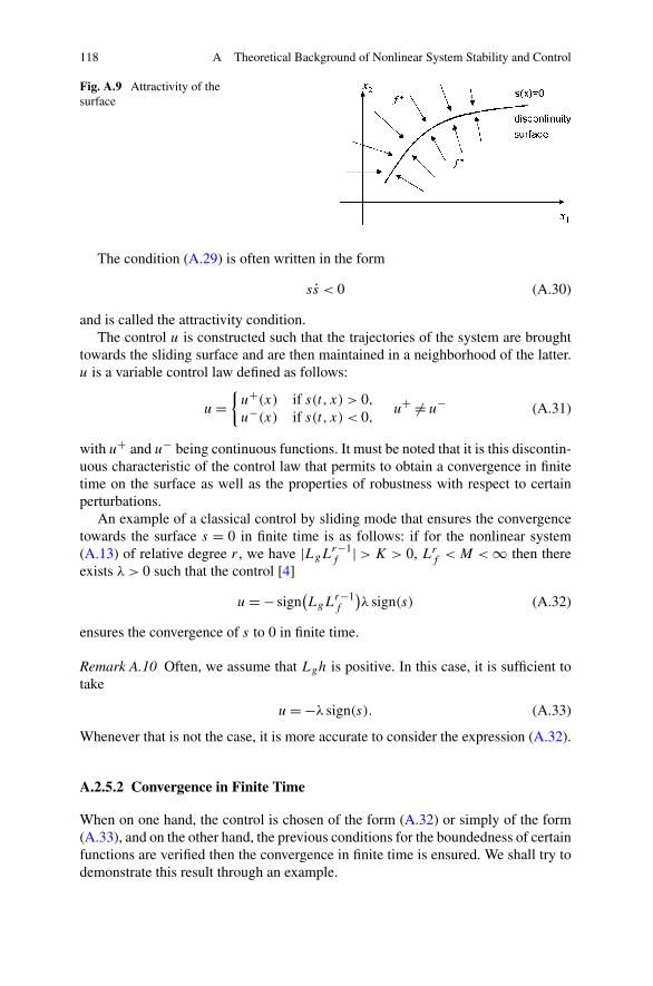
This condition translates the fact that, in a neighborhood of the sliding surface, thevelocity vectors of the trajectories of the system must point towards this surface, seeFig. A.9 [8].

Hence, once the surface is intersected, the trajectories stay in an ε-neighborhoodof S, and we say that the sliding mode is ideal if we have exactly s(t, x) = 0.


Fig. A.9 Attractivity of thesurface

The condition (A.29) is often written in the form

ss < 0 (A.30)

and is called the attractivity condition.The control u is constructed such that the trajectories of the system are brought

towards the sliding surface and are then maintained in a neighborhood of the latter.u is a variable control law defined as follows:

u ={

u+(x) if s(t, x) > 0,

u−(x) if s(t, x) < 0,u+ �= u− (A.31)

with u+ and u− being continuous functions. It must be noted that it is this discontin-uous characteristic of the control law that permits to obtain a convergence in finitetime on the surface as well as the properties of robustness with respect to certainperturbations.

An example of a classical control by sliding mode that ensures the convergencetowards the surface s = 0 in finite time is as follows: if for the nonlinear system(A.13) of relative degree r , we have |LgL

r−1f | > K > 0, Lr

f < M < ∞ then thereexists λ > 0 such that the control [4]

u = − sign(

LgLr−1f

)

λ sign(s) (A.32)

ensures the convergence of s to 0 in finite time.

Remark A.10 Often, we assume that Lgh is positive. In this case, it is sufficient totake

u = −λ sign(s). (A.33)

Whenever that is not the case, it is more accurate to consider the expression (A.32).

A.2.5.2 Convergence in Finite Time

When on one hand, the control is chosen of the form (A.32) or simply of the form(A.33), and on the other hand, the previous conditions for the boundedness of certainfunctions are verified then the convergence in finite time is ensured. We shall try todemonstrate this result through an example.


Example A.1 [4] Consider the following simple example:

x = b + u(A.34)

u = −λ sign(x − xd)

with xd the desired state, s = x − xd the sliding surface and λ > |b| + sup|xd |, thenx converges to xd in finite time and remains on the surface x = xd .

Proof

s = x − xd

s = b − λ sign(s) − xd

Consider the Lyapunov function: V = s2

2 . In this case, we have

V = s(

b − λ sign(s) − xd

)

if λ > |b| + sup|xd | then V < 0.Hence, the convergence is demonstrated. It now remains to show that the conver-

gence is achieved in finite time.Since V < 0, there exists a constant K > 0 such that V < −K|s|.Now V = s2

2 ⇒ |s| = √2V therefore V < −√

2K√

V ,Set K1 = −√

2K ⇒ V < −K1√

V , let us take the worst case where the maxi-mum convergence time is the limit case: V = −K1

√V

The solution of this equation gives

V −1/2dV = −K1dt

2V 1/2 = −K1t + V0

V (t) =(−K1t + V0

2

)2

The time from which V (t) = 0 corresponds to t = V0K1

, which is finite. �

A.2.5.3 The Chattering Phenomenon

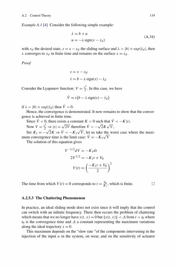
In practice, an ideal sliding mode does not exist since it will imply that the controlcan switch with an infinite frequency. There then occurs the problem of chatteringwhich means that we no longer have s(t, x) = 0 but ‖s(t, x)‖ < Δ from t > t0 wheret0 is the convergence time and Δ a constant representing the maximum variationsalong the ideal trajectory s = 0.

This maximum depends on the “slew rate ”of the components intervening in theinjection of the input u in the system, on wear, and on the sensitivity of actuator


Fig. A.10 Chatteringphenomenon

Fig. A.11 Saturationfunction

Fig. A.12 Sigmoid function

noise in the case of an analog control hence limiting the variation of speed betweenu+ and u−, see Fig. A.10. In the discrete case, the switching speed is limited bythe data measurement which is in turn constrained by the sampling period and thecomputation time [8].

This phenomenon constitutes a non-negligible disadvantage because even if it ispossible to filter the output of the process, it is susceptible to excite high-frequencymodes that were not taken into account in the model of the system. This can degradethe performances and even lead to instability [29].

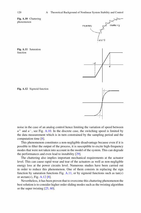
The chattering also implies important mechanical requirements at the actuatorlevel. This can cause rapid wear and tear of the actuators as well as non-negligibleenergy loss at the power circuits level. Numerous studies have been carried outin order to reduce this phenomenon. One of them consists in replacing the signfunction by saturation functions Fig. A.11, or by sigmoid functions such as tan(s)

or arctan(s), Fig. A.12 [8].Nevertheless, it has been proven that to overcome this chattering phenomenon the

best solution is to consider higher order sliding modes such as the twisting algorithmor the super twisting [25, 60].

A.3 Summary 121

Fig. A.13 Architecture ofmulti controllers

A.2.6 Control Design Technique Based on the Switching BetweenSeveral Controllers

The control design techniques based on the switching between several controllershave been the subject of intensive applications these last few years. The importanceof such methods comes from the existence of systems that are not stabilizable by asingle controller. In effect, a large range of dynamical systems is modeled by a fam-ily of continuous subsystems and a logic rule orchestrating the switching betweenthese subsystems, see Fig. A.13

Based on this, switching systems appear as a rigorous concept for studying com-plexes systems, even if their theoretical properties are still the subject of intensiveresearch.

A.3 Summary

This appendix has been devoted to the presentation of the theoretical aspects on sta-bility and control of nonlinear and switching systems. There is no general method-ology for the design of controller for nonlinear systems as opposed to controllerdesign for linear systems. Depending on the class of nonlinear systems under study,some approaches are better suited than others. In addition, we have attempted toexplain in a simple way the principle of some nonlinear control design techniquesthat fall within the scope of this book with the aim of using some of them for thestabilization of underactuated mechanical systems.

Appendix BLimits of Linearization and Dangersof Destabilization

A common practice of automatic community is to assume that a system can bedescribed by a set of differential equations around an operating point as follows:

x = Ax + Bu(B.1)

y = Cx

Assuming that (B.1) describes the system behavior, we can then exploit linear con-trol design procedures, where powerful analysis and design tools are available. How-ever, nonlinear system behaviors can be more complex than what can be representedby an equivalent linear model.

Neglecting such behaviors, unpredictable instability may arise and may causeperformance degradation. Moreover, the obtained linear system is valid only aroundthe considered operating point. Hence, it can describe the system only in the neigh-borhood of this point. On the other hand, some phenomena such as Coulomb fric-tion, backlash, and hysteresis, called hard nonlinearities, cannot be captured by lin-ear equations. Therefore, these nonlinearities are neglected.

Additional nonlinear phenomena include finite escape time, multiple equilibriumpoints, limit cycles, and chaos. A more complete description of these phenomenaand others is given in [18, 37].

To illustrate the impact of the loss of information due to linearization, let usconsider the following examples [20]:

Example B.1 Several equilibrium points:

x = −x + x2

(B.2)x(t = 0) = x0

After linearization around x(t) = 0, the obtained dynamic and associated solutionare given by

x = −x(t)(B.3)

x(t) = x0e(−t)


123

http://dx.doi.org/10.1007/978-3-319-02636-7

124 B Limits of Linearization and Dangers of Destabilization

Fig. B.1 Responses of anonlinear system for severalinitial conditions

Equation (B.3) indicates that for any initial condition x0, the solution exponen-tially converges towards the equilibrium point.

However, according to (B.2), the nonlinear system possesses a second equilib-rium point at x(t) = 1.

The impact of negligence of this point can be illustrated by calculating the solu-tion of the nonlinear system:

x(t) = x0e−t

1 + x0(e−t − 1)(B.4)

according to (B.4), note that:For x0 < 1, the solution tends to 0 when t → ∞ like for the linear case.For x0 > 1, the solution explodes to infinity in finite time, see Fig. B.1.

Example B.2 The linearized system is not controllable.Consider the following unicycle robot model (see [7] for other models):

⎡

⎣

x1x2x3

⎤

⎦ =⎡

⎣

cosx3 0sinx3 0

0 1

⎤

⎦

[

u1u2

]

(B.5)

Clearly, (B.5) is controllable while the linearized system around the pointx3(t) = 0 given by

⎡

⎣

x1x2x3

⎤

⎦ =⎡

⎣

1 00 00 1

⎤

⎦

[

u1u2

]

(B.6)

is not controllable for x2(t)!

Other examples of performance degradation are given in [20].

B Limits of Linearization and Dangers of Destabilization 125

On the other hand, the use of linear controller can sometimes lead to destabiliza-tion; for example, the consequence of the peaking phenomenon on a linear systemcan lead to the system instability [78, 80].

To illustrate this concept let us consider the partially linear coupled system de-scribed by the dynamics:

x = f (x, y)(B.7)

y = Ay + By

Let us make the following assumptions:

(b1) The pair (A,B) is supposed controllable.(b2) The nonlinear function f is differentiable to first order with respect to the time.(b3) The origin is an GAS equilibrium point for the zero dynamic x = f (x,0).

According to (B.7), and assumption (b3), it seems rather clear intuitively that alinear controller can be designed to lead the dynamics y(t) to 0 exponentially suchthat the zero dynamic of the nonlinear system is GAS. However, this strategy canlead the nonlinear dynamics to instability and its trajectory may escape to infinity infinite time. For example consider the following system:

Example B.3 Finite escape time:

x = −(1 + y2)

2x3 (B.8)

y1 = y2

y2 = u

From (B.8), one can verify that the assumption (b3) is satisfied.By designing a linear controller as follows:

u = −a2y1 − 2ay2 (B.9)

multiple eigenvalues for the closed system result at −a.Linear analysis tools can be used to find the exact solution y2(t) given by

y2 = −a2te−at (B.10)

and from this solution it appears that the dynamic |y2(t)| rises to a peak, then con-verges exponentially to 0. By computation, we can show that the peak time is t = 1

a.

From (B.10), we can conclude that for important values of a, y converges fastertowards 0. Hence, from assumption (b3), it seems that important values of a allowa fast stabilization of the nonlinear system.

Nevertheless, in [38], it was shown that this is not true. Indeed, if we substitute(B.10) in (B.8). By integrating, the resulting expression is given by

x2(t) = x20

1 + x20(t + (1 + at)e−at − 1)

(B.11)

126 B Limits of Linearization and Dangers of Destabilization

The peaking phenomenon destabilization effect is now apparent when we replacethe values of x0, a and t in (B.11). For example, for a = 10 and x2

0 = 2.176, theresponse x2(t ∼= 0.5) becomes unbounded and we have escape to infinity in finitetime.

Other examples and discussion of this phenomenon are in [38, 78, 80].

Appendix CA Little Differential Geometry

This section is devoted to the definition of some concepts and basic tools of dif-ferential geometry introduced in nonlinear automatic control theory, since the early1970s, by Eliott, Lobry, Hermann, Krener, Brockett, and others.

Diffeomorphism A diffeomorphism is a nonlinear change of coordinates z =Φ(x) where Φ is a vectorial function

Φ(x) =

⎛

⎜⎜⎜⎝

Φ1(x1, . . . , xn)

Φ2(x1, . . . , xn)...

Φn(x1, . . . , xn)

⎞

⎟⎟⎟⎠

with the following properties:

• Φ(x) is a bijective application• Φ(x) and Φ−1 are differentiable applications.

If these properties are verified for all x ∈ Rn then Φ is a global diffeomorphism.

Otherwise, Φ is a local diffeomorphism.

Proposition C.1 If the Jacobian matrix of Φ , evaluated at the point x = x0 isnonsingular, then Φ(x) is a local diffeomorphism.

Lie Derivative and Bracket Let f and g be two vector fields on an open Ω ofR

n with all continuous partial derivatives, and denote by ∂f∂x

and ∂g∂x

the Jacobianmatrices.

The Lie derivative of g along f is the vector field

Lf g = ∂g

∂xf.

The Lie bracket of f and g is the vector field

[f,g] = Lf g − Lgf.


127

http://dx.doi.org/10.1007/978-3-319-02636-7

128 C A Little Differential Geometry

We define also the vector fields

adff g = [f,g]adk

f g = [

f,adk−1f g

]

, k = 2,3, . . .

Distribution, Involutivity and Complete Integrability

• A distribution Δ on a manifold M assigns to each point x ∈ M a subspace of thetangent space T .

• A set of vectors {g1, . . . , gm} in Ω is said involutive if for all the i and j thebracket [gi, gj ] is a linear combination of vectors g1, . . . , gm, that is, there existfunctions αk

ij defined in Ω such that

[gi, gj ] =k=m∑

k=1

αkij gk.

That is, if for all the f and g in Δ, [f,g] belongs to Δ (Δ is closed by Liebracket).

• A set of linearly independent vectors {g1, . . . , gm} is a complete integrable set, ifthe system of n − m partial derivative equations

∂h

∂xg1 = 0, . . . ,

∂h

∂xgn−m = 0

admits a solution h : Ω → Rn such that ∂h

∂x�= 0

Theorem C.1 ([70] (Frobenius)) A set of linearly independent vectors {g1, . . . , gm}is involutive if and only if it is completely integrable.

For proof and examples see [37].

Relative Degree The relative degree associated with the system

x = f (x) + g(x)u(C.1)

y = h(x)

in a region Ω ⊂ Rn is given by the integer γ such that

Lgh(x) = LgLf h(x) = · · · = LgLγ−2f h(x) = 0

LgLγ−1f h(x) �= 0

for all x ∈ Ω .

Appendix DControllability of Continuous Systems

One of the main goals of automatic control is to establish control laws so that asystem evolves according to a predetermined objective. This requires controllabilityof the system. Intuitively, the controllability means that we can bring a system fromone state to another by means of a control. Conversely, non-controllability impliesthat some states are unreachable for any control.

D.1 Controllability of Linear Systems

For controlled linear systems

x = Ax + Bu (D.1)

y = Cx (D.2)

where An×n is the state matrix, x ∈Rn is the vector states, Bn×m the control matrix,

u controls belonging to a set of admissible controls U, Cp×n the output matrix andy ∈R

p the system outputs.

Definition D.1 [35] The system (D.1) is controllable if for each couple (x0, xd) ofR

n there exist a finite time T and a control u defined on [0, T ] that brings the systemfrom an initial state x(0) = x0 to a desired state x(T ) = xd .

D.1.1 Kalman Controllability Criterion

An algebraic characterization of linear systems controllability, due to Kalman, isgiven as follows:


129

http://dx.doi.org/10.1007/978-3-319-02636-7

130 D Controllability of Continuous Systems

Fig. D.1 Static statefeedback stabilization

Theorem D.1 The linear system (D.1) is controllable if and only if the rank of itscontrollability matrix

C = (

B AB . . . An−1B)

(D.3)

is equal to n. We say that the pair (A,B) is controllable.

Details and proofs can be found in [17].For controllable linear systems, we seek to design a controller that makes the

origin asymptotically stable. Several approaches are available, for example, we candesign control laws by state feedback.

D.1.2 State Feedback Stabilization

A linear state feedback or controller for (D.1) is a control law

u(t) = −Kx(t) (D.4)

where Km×n is a gain matrix.When the value of u(t) at t depends only on x(t) then the feedback is called

static feedback, Fig. D.1.The gain matrix can be computed in several ways, for example by pole place-

ment.

Pole Placement Design When a system is controllable, the pole placement prin-ciple consists of determining a control law u = −Kx such that σ(A − BK) = σd ,where σ is the spectrum of (A − BK) and σd is the desired spectrum.

The difficulty of this approach lies in the determination of the spectrum sincethere is no general methodology for doing so. This method offers the possibility toplace the closed-loop poles anywhere in the negative half-plane, regardless of theopen-loop poles location. As a result, the response time can be controlled. However,if the poles are placed too far into the negative half-plane, the values of the gain K

are very large and can cause saturation problems and can lead to instability.

Remark D.1 The control law u is designed assuming that the state vector x is avail-able. This assumption is not always true. Sometimes, some states are not available,

D.2 Controllability Concepts for Nonlinear Systems 131

because it is either difficult or impossible to physically measure these states or itis too expensive. In this case, we proceed to a reconstruction of the missing statesusing observers. However, throughout this book we are interested in the problem ofcontrol under the assumption that states are measurable.

D.2 Controllability Concepts for Nonlinear Systems

The notion of controllability which seems simple and intuitive for linear systemsis rather complicated for nonlinear systems where several definitions of the latterexist. The first results on nonlinear system controllability are due to Sussmann andJurdjevic [79], Lobry [48], Hermann and Krener [30], Sussmann [76, 77] and for anice presentation see also Nijmeijer and Van der Schaft [55].

A nonlinear system is generally represented by

x = f (x,u)(D.5)

y = h(x)

where x ∈ M ⊂ Rn, u ∈R

m, y ∈ Rp , and f,h are C∞.

Definition D.2 Let U be a subset of M and let (x0, xd) ∈ U . We say that xd isU -accessible from x0 which we denote by xdAux0, if there exist a measurable andbounded control u and a finite time T , such that the solution x(t) of (D.5), fort ∈ [0, T ], satisfies

x(0) = x0, x(T ) = xd and x ∈ U for t ∈ [0, T ]

we denote by A(x0) the set of points in M accessible from x0:

A(x0) = {x ∈ M/ xAMx0} (D.6)

Definition D.3 The system (D.5) is controllable at x0 if A(x0) = M and is control-lable if A(x0) = M for all x ∈ M .

When a system is controllable at x0, it may be necessary to cover a considerabledistance or time for reaching a point near x0. This leads us to introduce a localversion of the concept of controllability.

Definition D.4 The system (D.5) is said locally controllable at x0, if for all neigh-borhood U of x0, Au(x0) is a neighborhood of x0, where

Au(x0) = {x ∈ U/ xAux0} (D.7)

and it is said to be locally controllable if it is locally controllable for all x ∈ M .


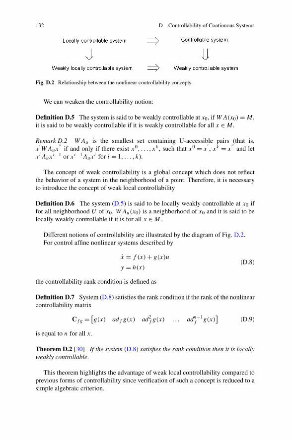
Fig. D.2 Relationship between the nonlinear controllability concepts

We can weaken the controllability notion:

Definition D.5 The system is said to be weakly controllable at x0, if WA(x0) = M ,it is said to be weakly controllable if it is weakly controllable for all x ∈ M .

Remark D.2 WAu is the smallest set containing U-accessible pairs (that is,x

′WAux

′′if and only if there exist x0, . . . , xk , such that x0 = x

′, xk = x

′′and let

xiAuxi−1 or xi−1Aux

i for i = 1, . . . , k).

The concept of weak controllability is a global concept which does not reflectthe behavior of a system in the neighborhood of a point. Therefore, it is necessaryto introduce the concept of weak local controllability

Definition D.6 The system (D.5) is said to be locally weakly controllable at x0 iffor all neighborhood U of x0, WAu(x0) is a neighborhood of x0 and it is said to belocally weakly controllable if it is for all x ∈ M .

Different notions of controllability are illustrated by the diagram of Fig. D.2.For control affine nonlinear systems described by

x = f (x) + g(x)u(D.8)

y = h(x)

the controllability rank condition is defined as

Definition D.7 System (D.8) satisfies the rank condition if the rank of the nonlinearcontrollability matrix

Cfg = [

g(x) adf g(x) ad2f g(x) . . . adn−1

f g(x)]

(D.9)

is equal to n for all x.

Theorem D.2 [30] If the system (D.8) satisfies the rank condition then it is locallyweakly controllable.

This theorem highlights the advantage of weak local controllability compared toprevious forms of controllability since verification of such a concept is reduced to asimple algebraic criterion.

References 133

References

1. D.V. Anosov, On stability of equilibrium points of relay systems. J. Autom. Remote Control2,135–149 (1959)

2. P.J. Antsalkis, A.N. Michel, Linear Systems (McGraw-Hill, New York, 1997)3. J-P. Aubin, H. Frankowska, Set-Valued Analysis (Birkhäuser, Basel, 1990)4. J.P. Barbot, Systèmes à structure variable. Technical report, École Nationale Supérieure

d’Electronique et de Ses Applications, ENSEA, France, 20095. N. Bedrossian, Approximate feedback linearisation: the cart pole example, in Proc. IEEE Int.

Conf. on Robotics and Automation (1992), pp. 1987–19926. I. Belgacem, Automates hybrides Zénon: Exécution-simulation. Master at Aboubekr Belkaid

University, Tlemcen, Algeria, 20097. A.M. Bloch, M. Reyhanoglu, N.H. McClamroch, Control and stabilization of nonholonomic

dynamic systems. IEEE Trans. Autom. Control 37(11),1746–1757 (1992)8. T. Boukhobza, Contribution aux formes d’observabilité pour les observateurs à modes glis-

sants. Ph.D. thesis, Paris Sud Centre d’Orsay University, France, 19979. M.S. Branicky, Stability of switched and hybrid systems, in Proc. 33rd IEEE Conf. on Decision

and Control, USA (1994), pp. 3498–350310. M.S. Branicky, Studies in hybrid systems: modeling, analysis, and control. Ph.D. thesis, De-

partement of Electrical and Computer Engineering, Massachusetts Institute of Technology,1995

11. M.S. Branicky, Stability of hybrid systems: State of the art, in Proc. 36th IEEE Conf. onDecision and Control, USA (1997), pp. 120–125

12. M.S. Branicky, Multiple Lyapunov functions and other analysis tools for switched and hybridsystems. IEEE Trans. Autom. Control 43(4), 475–482 (1998)

13. R.W. Brockett, Asymptotic Stability and Feedback Stabilization (Birkhäuser, Basel, 1983)14. K. Busawon, Lecture notes in control systems engineering. Technical report, Northumbria

University, Newcastle, United Kingdom, 200815. S. Canudas, G. Bastin, Theory of Robot Control (Springer, Berlin, 1996)16. G. Chesi, Y.S. Hung, Robust commutation time for switching polynomial systems, in Proc.

46th IEEE Conf. on Decision and Control, USA (2007)17. B. D’Andréa Novel, M.C. De-Lara, Commande Linéaire des Systèmes Dynamiques (École des

Mines Press, 2000)18. H. Dang Vu, C. Delcarte, Bifurcation et Chaos (Ellipses edition, 2000)19. R. DeCarlo, M. Branicky, S. Petterssond, B. Lennartson, Perspectives and results on the sta-

bility and stabilizability of hybrid systems. Proc. IEEE 88, 1069–1082 (2000)20. W.E. Dixon, A. Behal, D. Dawson, S. Nagarkatti, Nonlinear Control of Engineering Systems

(Birkhäusser, Basel, 2003)21. S.V. Emel’yanov, Variable Structure Control Systems (Nauka, Moscow, 1967)22. A.G. Fillipov, Differential Equations with Discontinuous Right Hand-Sides. Mathematics and

its Applications (Kluwer Academic, Dordrecht, 1983)23. T. Floquet, Contributions à la commande par modes glissants d’ordre supérieur. Ph.D. thesis,

University of Sciences and Technology of Lille, France, 200024. G.F. Franklin, J.D. Powell, A. Emami-Naeini. Feedback Control of Dynamic Systems

(Prentice-Hall, Englewood Cliffs, 2002)25. L. Fridman, A. Levant, Sliding Modes of Higher Order as a Natural Phenomenon in Control

Theory (Springer, Berlin, 1996)26. L. Gurvits, R. Shorten, O. Mason, On the stability of switched positive linear systems. IEEE

Trans. Autom. Control 52, 1099–1103 (2007)27. J. Hauser, Nonlinear control via uniform system approximation. Syst. Control Lett. 17, 145–

154 (1991)


28. J. Hauser, S. Sastry, P. Kokotovic, Nonlinear control via approximate input-output lineariza-tion. IEEE Trans. Autom. Control 37(3), 392–398 (1992)

29. B. Heck, Sliding mode control for singulary perturbed systems. Int. J. Control 53(4) (1991)30. R. Hermann, A.J. Krener, Nonlinear controllability and observability. IEEE Trans. Autom.

Control 22, 728–740 (1977)31. L.R. Hunt, R. Su, G. Meyer Gurvits, R. Shorten, O. Mason, Global transformations of nonlin-

ear systems. IEEE Trans. Autom. Control 28(1), 24–31 (1983)32. A. Isidori, Nonlinear Control Systems (Springer, Berlin, 1995)33. B. Jakubczyk, W. Respondek, On linearisation of control systems. Rep. Sci. Pol. Acad. 28(9),

517–522 (1980)34. J. Jouffroy, Stabilité et systèmes non linéaire: réflexion sur l’analyse de contraction. Ph.D.

thesis, Savoie University, France, 200235. T. Kailath, Linear Systems (Prentice-Hall, Englewood Cliffs, 1981)36. W. Kang, Approximate linearisation of nonlinear control systems, in Proc. IEEE Conf. on

Decision and Control (1993), pp. 2766–177137. H.K. Khalil, Nonlinear Systems (Prentice-Hall, Englewood Cliffs, 2002)38. P. Kokotovic, The joy of feedback: Nonlinear and adaptive. IEEE Control Syst. Mag. 12(3),

7–17 (1992)39. A.J. Krener, Approximate linearisation by state feedback and coordinate change. Syst. Control

Lett. 5, 181–185 (1984)40. A.J. Krener, M. Hubbard, S. Karaban, B. Maag, Poincaré’s Linearisation Method Applied to

the Design of Nonlinear Compensators (Springer, Berlin, 1991)41. M. Kristic, P. Kokotovic, Nonlinear and Adaptive Control Design (Wiley, New York, 1995)42. H. Kwakernak, R. Sivan, Linear Optimal Control Systems (Library of Congress, 1972)43. H.G. Kwatny, G.L. Blankenship, Nonlinear Control and Analytical Mechanics: A Computa-

tional Approach (Birkhäuser, Basel, 2000)44. F. Lamnabhi Lagarrique, P. Rouchon, Commandes Non Linéaires (Lavoisier, Paris, 2003)45. M. Latfaoui, Linéaisation approximative par feedback. Master at Aboubekr Belkaid Univer-

sity, Tlemcen, Algeria, 200246. J. Lévine, Analyse et commande des systèmes non linéaires. Technical report, École des Mines

de Paris, France, 200447. D. Liberzon, A.S. Morse, Basic problems in stability and design of switched systems. IEEE

Control Syst. Mag. 19(5), 59–70 (1999)48. C. Lobry, Contrôlabilité des Systèmes Non Linéaires (CNRS, Paris, 1981)49. D.G. Luenberger, Introduction to Dynamic Systems (Wiley, New York, 1979)50. N. Manamanni, Aperçu rapide sur les systèmes hybrides continus. Technical report, University

of Reims, France, 200751. M. Margaliot, M.S. Branicky, Nice reachability for planar bilinear control systems with appli-

cations to planar linear switched systems. IEEE Trans. Autom. Control (May 2008)52. O. Mason, R. Shorten, A conjecture on the existence of common quadratic Lyapunov functions

for positive linear systems, in Proc. American Control Conf., USA (2003), pp. 4469–447053. S. Mastellone, D.M. Stipanovic, M.W. Spong, Stability and convergence for systems with

switching equilibria, in Proc. 46th IEEE Conf. on Decision and Control, USA (2007),pp. 4013–4020

54. A.N. Michel, L. Hou, Stability results involving time-averaged Lyapunov function derivatives.J. Nonlinear Anal., Hybrid Syst. 3(1), 51–64 (2009)

55. H. Nijmeijer, A. van der Schaft, Nonlinear Dynamical Control Systems (Springer, Berlin,1990)

56. K. Ogata, Modern Control Engineering (Prentice-Hall, Englewood Cliffs, 1997)57. R. Ortega, A. Loria, P. Nicklasson, H. Sira-Ramirez, Passivity-Based Control of Euler La-

grange Systems (Springer, Berlin, 1998)

References 135

58. P. Peleties, Modeling and design of interacting continuous-time/discrete event systems. Ph.D.thesis, Electrical Engineering, Purdue Univ., West Lafayette, IN, 1992

59. P. Peleties, R.A. DeCarlo, Asymptotic stability of m-switched systems using Lyapunov-likefunctions, in Proc. American Control Conf., USA (1991), pp. 1679–1684

60. W. Perruquetti, J.P. Barbot, Sliding Mode Control in Engineering (Taylor and Francis, London,2002)

61. V.M. Popov, Absolute stability of nonlinear control systems of automatic control. J. Autom.Remote Control 22, 857–875 (1962)

62. J.P. Richard, Mathématiques pour les Systèmes Dynamiques (Lavoisier, Paris, 2002)63. H. Saadaoui, Contribution à la synthèse d’observateurs non linéaires pour des classes de sys-

tèmes dynamiques hybrides. Ph.D. thesis, Cergy Pontoise University, France, 200764. R.G. Sanfelice, A.R. Teel, R. Sepulchre, A hybrid systems approach to trajectory tracking con-

trol for juggling systems, in Proc. 46th IEEE Conf. on Decision and Control, USA (2007), pp.5282–5287

65. T. Sari, C. Lobry, Contrôle Non Linéaire et Applications (Hermann, Paris, 2005)66. S.S. Sastry, Nonlinear Systems: Analysis, Stability and Control (Springer, Berlin, 1999)67. R. Sepulchre, M. Jankovic, P. Kokotovic, Contructive Nonlinear Control (Springer, Berlin,

1997)68. C. Shen, Q. Wei, F. Shumin, On exponential stability of switched systems with delay: multiple

Lyapunov functions approach, in Proc. Chineese Control Conf., China (2007), pp. 664–66869. H. Sira Ramirez, Sliding regimes in general nonlinear systems: a relative degree approach. Int.

J. Control 50(4), 1487–1506 (1989)70. J. Slotine, W. Li, Nonlinear Systems Analysis (Prentice-Hall, Englewood Cliffs, 1993)71. E.D. Sontag, Y. Wang, On characterizations of the input-to-state stability property. Syst. Con-

trol Lett. 24, 351–359 (1995)72. S.K. Spurgeon, C. Edwards, Sliding Mode Control: Theory and Applications (Taylor and Fran-

cis, London, 1983)73. T. Sugie, K. Fujimoto, Control of inverted pendulum systems based on approximate linearisa-

tion, in Proc. IEEE Conf. on Decision and Control (1994), pp. 1647–164974. Z. Sun, S.S. Ge, Analysis and synthesis of switched linear control systems. Automatica 41,

181–195 (2005)75. Z. Sun, S.S. Ge, Switched Linear Systems (Springer, Berlin, 2005)76. H.J. Sussmann, Lie Brackets, Real Analyticity and Geometric Control (Birkhäuser, Basel,

1983)77. H.J. Sussmann, A general theorem on local controllability. SIAM J. Control Optim. 25(1),

158–194 (1987)78. H.J. Sussmann, Limitations on stabilizability of globally minimum phase systems. IEEE

Trans. Autom. Control 35(1), 117–119 (1990)79. H.J. Sussmann, V. Jurdjevic, Controllability of nonlinear systems. J. Differ. Equ. 12(2), 95–

116 (1991)80. H.J. Sussmann, P. Kokotovic, The peaking phenomenon and the global stabilization of nonlin-

ear systems. IEEE Trans. Autom. Control 36(4), 424–440 (1991)81. C.J. Tomlin, J. Lygeros, S. Sastry, Introduction to Dynamic Systems (Springer, Berlin, 2003)82. Y.Z. Tzypkin, Theory of Control of Relay Systems (Gostekhizdat, Moscow, 1955)83. V.I. Utkin, Variable structure systems with sliding mode. IEEE Trans. Autom. Control 22(2),

212–222 (1977)84. V.I. Utkin, Sliding Modes in Control Optimization (Springer, Berlin, 1992)85. A. van der Schaft, H. Schumacher, An Introduction to Hybrid Dynamical Systems (Springer,

Berlin, 2002)86. A. van der Shaft, L2 Gain and Passivity Techniques in Nonlinear Control (Springer, Berlin,

2000)


87. M. Vidyasagar, Nonlinear Systems Analysis (Prentice-Hall, Englewood Cliffs, 1993)88. D.A. Voytsekhovsky, R.M. Hirschorn, Stabilization of single-input nonlinear systems using

higher order compensating sliding mode control, in Proc. 45th IEEE Conf. on Decision andControl and the European Control Conf. (2005), pp. 566–571

89. J.C. Willems, Dissipative dynamical systems. Rational mechanics and analysis 45, 321–393(1972)

90. X. Xu, G. Zhai, Practical stability and stabilization of hybrid and switched systems. IEEETrans. Autom. Control 50(11), 1897–1903 (2005)

91. H. Ye, A.N. Michel, L. Hou, Stability analysis of discontinuous dynamical systems with ap-plication, in 13th IFAC Congress, USA (1996), pp. 461–466

92. H. Ye, A.N. Michel, L. Hou, Stability theory for hybrid dynamical systems. IEEE Trans. Au-tom. Control 43(4), 461–474 (1998)

93. S.H. Zak, Systems and Control (Oxford University Press, London, 2003)94. G. Zames, On the input-output stability of nonlinear time-varying feedback systems. IEEE

Trans. Autom. Control 11(2), 228–238 (1966)95. G. Zhai, B. Hu, K. Yasuda, A.N. Michel, Stability analysis of switched systems with stable

and unstable subsystems: an average dwell time approach, in Proc. American Control Conf.,USA (2000), pp. 200–204

96. G. Zhai, D. Liu, J. Imae, T. Kobayashi, Lie algebraic stability analysis for switched systemswith continuous-time and discrete-time subsystems. IEEE Trans. Circ. Syst. 53(2), 152–156(2006)

97. G. Zhai, H. Lin, X. Xu, A.N. Michel, Stability analysis and design of switched of normalsystems, in Proc. 43rd IEEE Conf. on Decision and Control, USA (2004), pp. 3253–3258

98. G. Zhai, I. Matsune, J. Imae, T. Kobayashi, A note on multiple Lyapunov functions and sta-bility condition for switched and hybrid systems, in Proc. 16th IEEE Int. Conf. on ControlApplication, Singapore (2007), pp. 1189–1199

99. J. Zhao, D.J. Hill, Dissipativity theory for switched systems. IEEE Trans. Autom. Control53(4), 941–953 (2008)

Index

AAcrobot, 8, 9, 18, 27, 29, 42, 47, 64, 65Approximation

high order, 83, 85, 112linear, 97, 106

BBackstepping, 10, 11, 35, 40, 44, 49, 55, 64,

114Ball and beam, 8, 18, 27, 31, 43, 48, 64, 83,

85BIBS, 56Brockett, 8, 10, 21, 22, 71Brunovsky form, 107, 112

CCentrifugal term, 16CFD, 10, 35, 40, 55, 65Chaos, 123Chattering, 88, 119Christoffel symbols, 16Classification, 10, 35, 43, 55

class I, 47class II, 47, 48

Complete integrability, 128Constraint

holonomic, 19, 27non-holonomic, 18, 27, 37

Controllability, 8, 17, 21–23, 40, 108, 129,131

Coriolis, 16

DDegree of complexity, 36, 40Diffeomorphism, 108, 109, 127Distribution, 128

EEnergy, 9, 113

kinetic, 16potential, 16, 28, 29

Euler–Lagrange equation, 15, 17, 19, 27,65

Equilibrium, 94

FFinite time convergence, 84, 118Forwarding, 10, 11, 44, 49Frobenius theorem, 109, 128Function

Chetaev, 99Lipscitzian, 94Lyapunov, 64, 97

common, 101multiples, 74, 101weak, 102

GGeneralized momentum, 27, 50

HHurwitz, 84

IInertial wheel pendulum, 9, 30, 65Inverted pendulum, 8, 9, 18, 28, 42, 48, 49, 65,

67Involutivity, 128

JJacubezyk–Respondek theorem, 108

KKalman criterion, 129


137

http://dx.doi.org/10.1007/978-3-319-02636-7

138 Index

LLagrange vector of multipliers, 19LaSalle invariance principle, 98Legendre

normal form, 17transformation, 16

Liebracket, 127derivative, 127

Limit cycles, 123Linearization

approximate, 82, 83, 110feedback, 23, 40, 56, 107input–output, 108input–state, 107limits, 123partial, 23, 43, 66, 68, 81, 109

collocated, 24coupled inputs, 25non-collocated, 24

LQR, 9, 71

NNormal form, 109

feedforward, 11, 48, 50, 53non-triangular, 11, 53non-triangular quadratic, 50strict feedback, 11, 45–48, 50, 53, 66

OObservability, 17

PPassivity, x, 8, 9, 113Peaking phenomenon, 56, 125Pendubot, 8, 9, 18, 27, 29, 42, 48, 64, 65, 67Pendular systems, 64Pole placement, 9, 71, 80, 130

RReduction, 49Relative degree, 8, 21, 40, 41, 43, 108, 109

robust, 111Robot

flexible, 8, 18joint elasticity, 41, 64walking biped, 10wheeled, 18

SSatellites, 8, 18, 27Sliding mass on cart, 41, 64Sliding mode, 10, 116Stability, 93, 94

asymptotic, 96

equilibrium, 95, 96exponential, 96global, 96switching system, x, 100

Stabilization, 8, 10, 11feedback, 130local, x, 106of a system, x, 105

Structural properties, 8, 10, 19, 35, 50Structure

chain, 10, 35, 39–41, 55isolated vertex, 10, 35, 39, 40, 43, 55, 82tree, 10, 35, 39, 40, 42, 55, 64, 78

Switch, 9, 71Switching control, 10, 71Symmetry, 26

kinetic, 27, 47, 49System

aeronautic, 18aeronautical, 7, 26, 27autonomous, 94chain, 20Lagrangian, 18, 26marine, 8, 18mechanical, 7, 27

fully actuated, 21underactuated, 10, 27, 35

minimum phase, 110mobile, 8non-autonomous, 94non-minimum phase, 21, 110nonlinear, 15, 19, 66, 96, 106spatial, 7switching, 121

TTora, 8, 9, 18, 27, 29, 42, 47, 64, 65, 67Trajectory tracking, 10, 57, 105Triangular form, 114Two order sliding mode, 88

UUnder water vehicles, 19Underactuated mechanical systems, 55Unicycle, 18, 20, 124

VVariable

external, 27, 47, 49shape, 27, 47, 49, 50, 90

VTOL, 9

ZZero dynamics, 17, 56, 110

Date post:	31-Mar-2022
Category:	Documents
Upload:	others
View:	1 times
Download:	0 times

Appendix A Theoretical Background of Nonlinear System ...

Documents