If the speed of a body is given, then its size and the direction need to be identified.For the description of such a directional quantity, vectors are used. These vectorsin the three dimensional space require three components which, e.g. in a columnvector, are summarized as follows:
v =⎛⎝
v1v2v3
⎞⎠ . (A.1)
A second possibility is to present a transposed column vector
vᵀ = (v1 v2 v3
), (A.2)
a row vector.In another way, we get the concept of the vector when the following purely math-
ematical problem is considered: Find the solutions of the three coupled equationswith four unknowns x1, x2, x3 and x4:
and the coefficients aij are included into the matrix
Adef=
⎛⎝
a11 a12 a13 a14a21 a22 a23 a24a31 a32 a33 a34
⎞⎠ . (A.8)
With the two vectors x and y and the matrix A, the system of equations can com-pactly be written as
Ax = y. (A.9)
If the two systems of equations
a11x1 + a12x2 = y1, (A.10)
a21x1 + a22x2 = y2 (A.11)
and
a11z1 + a12z2 = v1, (A.12)
a21z1 + a22z2 = v2 (A.13)
are added, one obtains
a11(x1 + z1) + a12(x2 + z2) = (y1 + v1), (A.14)
a21(x1 + z1) + a22(x2 + z2) = (y2 + v2). (A.15)
With the aid of vectors and matrices, the two systems of equations can be written as
Ax = y and Az = v. (A.16)
Adding the two equations in (A.16) is formally accomplished as
Ax + Az = A(x + z) = y + v. (A.17)
A comparison of (A.17) with (A.14) and (A.15) suggests the following definition ofthe addition of vectors:
A.2 Matrices 147
Definition:
y + v =
⎛⎜⎜⎜⎝
y1y2...
yn
⎞⎟⎟⎟⎠ +
⎛⎜⎜⎜⎝
v1v2...
vn
⎞⎟⎟⎟⎠
def=
⎛⎜⎜⎜⎝
y1 + v1y2 + v2
...
yn + vn
⎞⎟⎟⎟⎠ . (A.18)
Accordingly, the product of a vector and a real or complex number c is defined by
Definition:
c · x def=⎛⎜⎝
c · x1...
c · xn
⎞⎟⎠ . (A.19)
A.2 Matrices
A.2.1 Types of Matrices
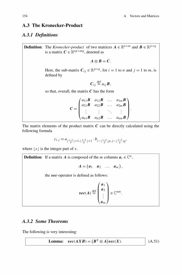
In the first section, the concept of the matrix has been introduced.
Definition: If a matrix A has n rows and m columns, it is called an n×m matrixand denoted A ∈ R
n×m.
Definition: If A (with the elements aij ) is an n×m matrix, then the transpose ofA, denoted by Aᵀ, is the m × n matrix with the elements a
ᵀij = aji .
So the matrix (A.8) has the matrix transpose
Aᵀ =
⎛⎜⎜⎝
a11 a21 a31a12 a22 a32a13 a23 a33a14 a24 a34
⎞⎟⎟⎠ . (A.20)
In a square matrix, one has n = m; and in an n×n diagonal matrix, all the elementsaij , i �= j , outside the main diagonal are equal to zero. An identity matrix I is adiagonal matrix where all elements on the main diagonal are equal to one. An r × r
identity matrix is denoted by I r . If a transposed matrix Aᵀ is equal to the originalmatrix A, such a matrix is called symmetric. In this case, aij = aji .
If, on the other hand, we formally insert the right-hand side of (A.23) into the leftequation, we obtain
y = ABzdef= Cz. (A.24)
150 A Vectors and Matrices
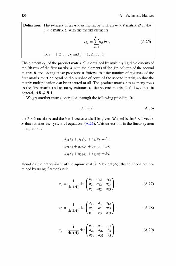
Definition: The product of an n × m matrix A with an m × � matrix B is then × � matrix C with the matrix elements
cij =m∑
k=1
aikbkj , (A.25)
for i = 1,2, . . . , n and j = 1,2, . . . , �.
The element cij of the product matrix C is obtained by multiplying the elements ofthe ith row of the first matrix A with the elements of the j th column of the secondmatrix B and adding these products. It follows that the number of columns of thefirst matrix must be equal to the number of rows of the second matrix, so that thematrix multiplication can be executed at all. The product matrix has as many rowsas the first matrix and as many columns as the second matrix. It follows that, ingeneral, AB �= BA.
We get another matrix operation through the following problem. In
Ax = b, (A.26)
the 3 × 3 matrix A and the 3 × 1 vector b shall be given. Wanted is the 3 × 1 vectorx that satisfies the system of equations (A.26). Written out this is the linear systemof equations:
a11x1 + a12x2 + a13x3 = b1,
a21x1 + a22x2 + a23x3 = b2,
a31x1 + a32x2 + a33x3 = b3.
Denoting the determinant of the square matrix A by det(A), the solutions are ob-tained by using Cramer’s rule
x1 = 1
det(A)det
⎛⎝
b1 a12 a13b2 a22 a23b3 a32 a33
⎞⎠ , (A.27)
x2 = 1
det(A)det
⎛⎝
a11 b1 a13a21 b2 a23a31 b3 a33
⎞⎠ , (A.28)
x3 = 1
det(A)det
⎛⎝
a11 a12 b1a21 a22 b2a31 a32 b3
⎞⎠ . (A.29)
A.2 Matrices 151
If we develop in (A.27) the determinant in the numerator with respect to the firstcolumn, we obtain
x1 = 1
det(A)
(b1 det
(a22 a23a32 a33
)− b2 det
(a12 a13a32 a33
)+ b3 det
(a12 a13a22 a23
))
= 1
det(A)(b1A11 + b2A21 + b3A31)
= 1
det(A)
(A11 A21 A31
)b. (A.30)
Accordingly, we obtain from (A.28) and (A.29)
x2 = 1
det(A)
(A12 A22 A32
)b (A.31)
and
x3 = 1
det(A)
(A13 A23 A33
)b. (A.32)
Here the adjuncts Aij are the determinants which are obtained when the ith rowand the j th column of the matrix A are removed, and from the remaining matrix thedeterminant is computed and this is multiplied by the factor (−1)i+j .
Definition: The adjuncts are summarized in the adjoint matrix
adj(A)def=
⎛⎝
A11 A21 A31A12 A22 A32A13 A23 A33
⎞⎠ . (A.33)
With this matrix, the three equations (A.30) to (A.32) can be written as one equation
x = adj(A)
det(A)b. (A.34)
Definition: The n × n matrix (whenever det(A) �= 0)
A−1 def= adj(A)
det(A)(A.35)
is called the inverse matrix of the square n × n matrix A.
For a matrix product, the inverse matrix is obtained as
(AB)−1 = B−1A−1 (A.36)
because
(AB)(B−1A−1) = A
(BB−1)A−1 = AA−1 = I .
152 A Vectors and Matrices
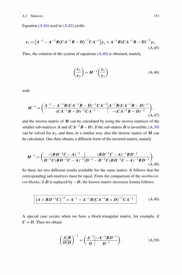
A.2.3 Block Matrices
Often large matrices have a certain structure, e.g. when one or more sub-arrays arezero matrices. On the other hand, one can make a block matrix from each matrixby drawing vertical and horizontal lines. For a system of equations, one then, forexample, obtains
⎛⎜⎜⎜⎝
A11 A12 · · · A1n
A21 A22 · · · A2n
......
. . ....
Am1 Am2 · · · Amn
⎞⎟⎟⎟⎠
⎛⎜⎜⎜⎜⎜⎝
x1
x2
...
xn
⎞⎟⎟⎟⎟⎟⎠
=
⎛⎜⎜⎜⎜⎜⎝
y1
y2
...
ym
⎞⎟⎟⎟⎟⎟⎠
. (A.37)
The Aij ’s are called sub-matrices and the vectors xi and yi sub-vectors. For twoappropriately partitioned block matrices, the product may be obtained by simplycarrying out the multiplication as if the sub-matrices were themselves elements:
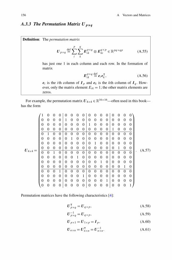
Permutation matrices have the following characteristics [4]:
Uᵀp×q = Uq×p, (A.58)
U−1p×q = Uq×p, (A.59)
Up×1 = U1×p = Ip, (A.60)
Un×n = Uᵀn×n = U−1
n×n. (A.61)
A.4 Derivatives of Vectors/Matrices with Respect to Vectors/Matrices 157
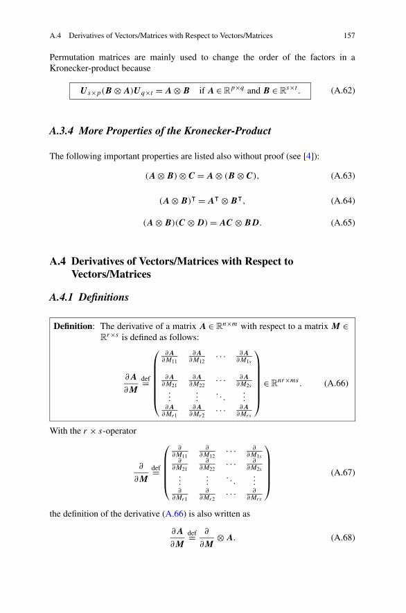
Permutation matrices are mainly used to change the order of the factors in aKronecker-product because
U s×p(B ⊗ A)Uq×t = A ⊗ B if A ∈ Rp×q and B ∈ R
s×t . (A.62)
A.3.4 More Properties of the Kronecker-Product
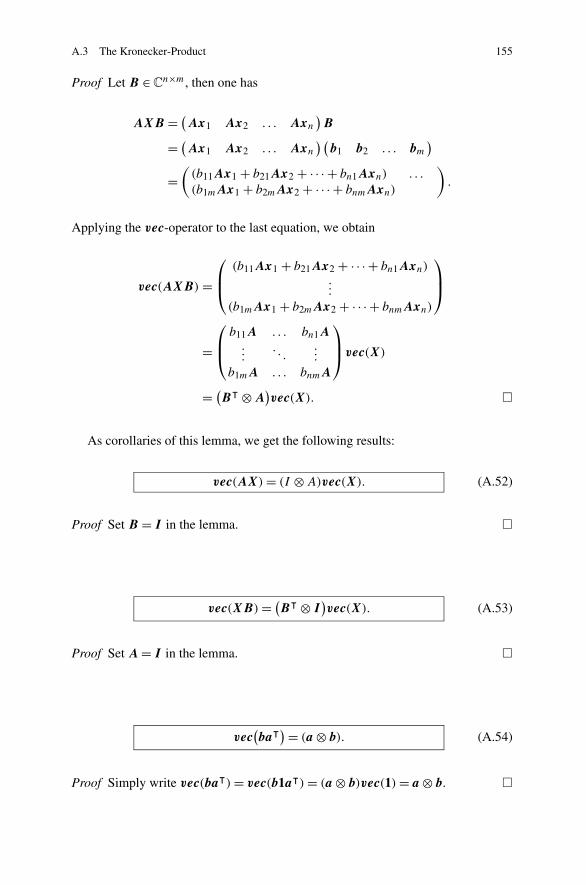
The following important properties are listed also without proof (see [4]):
(A ⊗ B) ⊗ C = A ⊗ (B ⊗ C), (A.63)
(A ⊗ B)ᵀ = Aᵀ ⊗ Bᵀ, (A.64)
(A ⊗ B)(C ⊗ D) = AC ⊗ BD. (A.65)
A.4 Derivatives of Vectors/Matrices with Respect toVectors/Matrices
A.4.1 Definitions
Definition: The derivative of a matrix A ∈ Rn×m with respect to a matrix M ∈
Rr×s is defined as follows:
∂A
∂M
def=
⎛⎜⎜⎜⎜⎜⎜⎝
∂A∂M11
∂A∂M12
· · · ∂A∂M1s
∂A∂M21
∂A∂M22
· · · ∂A∂M2s
......
. . ....
∂A∂Mr1
∂A∂Mr2
· · · ∂A∂Mrs
⎞⎟⎟⎟⎟⎟⎟⎠
∈ Rnr×ms. (A.66)
With the r × s-operator
∂
∂M
def=
⎛⎜⎜⎜⎜⎝
∂∂M11
∂∂M12
· · · ∂∂M1s
∂∂M21
∂∂M22
· · · ∂∂M2s
......
. . ....
∂∂Mr1
∂∂Mr2
· · · ∂∂Mrs
⎞⎟⎟⎟⎟⎠
(A.67)
the definition of the derivative (A.66) is also written as
∂A
∂M
def= ∂
∂M⊗ A. (A.68)
158 A Vectors and Matrices
Thus one can show that
(∂A
∂M
)ᵀ=
(∂
∂M⊗ A
)ᵀ=
((∂
∂M
)ᵀ⊗ Aᵀ
)= ∂Aᵀ
∂Mᵀ . (A.69)
For the derivatives of vectors with respect to vectors one has:
∂f ᵀ
∂p
def= ∂
∂p⊗ f ᵀ =
⎛⎜⎜⎜⎜⎜⎝
∂f ᵀ∂p1∂f ᵀ∂p2...
∂f ᵀ∂pr
⎞⎟⎟⎟⎟⎟⎠
=
⎛⎜⎜⎜⎜⎜⎝
∂f1∂p1
∂f2∂p1
· · · ∂fn
∂p1∂f1∂p2
∂f2∂p2
· · · ∂fn
∂M2...
.... . .
...∂f1∂pr
∂f2∂pr
· · · ∂fn
∂ps
⎞⎟⎟⎟⎟⎟⎠
∈ Rr×n (A.70)
and
∂f
∂pᵀdef= ∂
∂pᵀ ⊗ f =(
∂
∂p⊗ f ᵀ
)ᵀ=
(∂f ᵀ
∂p
)ᵀ∈ R
n×r . (A.71)
A.4.2 Product Rule
Let A = A(α) and B = B(α). Then we obviously have
∂(AB)
∂α= ∂A
∂αB + A
∂B
∂α. (A.72)
In addition, (A.66) can be rewritten as:
∂A
∂M=
∑i,k
Es×tik ⊗ ∂A
∂mik
, M ∈ Rs×t . (A.73)
Using (A.72) and (A.73), this product rule can be derived:
∂(AB)
∂M=
∑i,k
Es×tik ⊗ ∂(AB)
∂mik
=∑i,k
Es×tik ⊗
(∂A
∂mik
B + A∂B
∂mik
)
=(
∂
∂M⊗ A
)(I t ⊗ B) + (I s ⊗ A)
(∂
∂M⊗ B
)
= ∂A
∂M(I t ⊗ B) + (I s ⊗ A)
∂B
∂M. (A.74)
A.5 Differentiation with Respect to Time 159
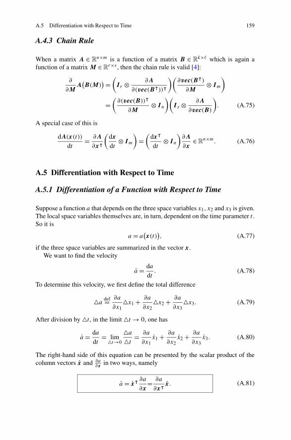
A.4.3 Chain Rule
When a matrix A ∈ Rn×m is a function of a matrix B ∈ R
k×� which is again afunction of a matrix M ∈ R
r×s , then the chain rule is valid [4]:
∂
∂MA
(B(M)
) =(
I r ⊗ ∂A
∂(vec(Bᵀ))ᵀ
)(∂vec(Bᵀ)
∂M⊗ Im
)
=(
∂(vec(B))ᵀ
∂M⊗ In
)(I s ⊗ ∂A
∂vec(B)
). (A.75)
A special case of this is
dA(x(t))
dt= ∂A
∂xᵀ
(dx
dt⊗ Im
)=
(dxᵀ
dt⊗ In
)∂A
∂x∈ R
n×m. (A.76)
A.5 Differentiation with Respect to Time
A.5.1 Differentiation of a Function with Respect to Time
Suppose a function a that depends on the three space variables x1, x2 and x3 is given.The local space variables themselves are, in turn, dependent on the time parameter t .So it is
a = a(x(t)
), (A.77)
if the three space variables are summarized in the vector x.We want to find the velocity
a = da
dt. (A.78)
To determine this velocity, we first define the total difference
�adef= ∂a
∂x1�x1 + ∂a
∂x2�x2 + ∂a
∂x3�x3. (A.79)
After division by �t , in the limit �t → 0, one has
a = da
dt= lim�t→0
�a
�t= ∂a
∂x1x1 + ∂a
∂x2x2 + ∂a
∂x3x3. (A.80)
The right-hand side of this equation can be presented by the scalar product of thecolumn vectors x and ∂a
∂x in two ways, namely
a = xᵀ ∂a
∂x= ∂a
∂xᵀ x. (A.81)
160 A Vectors and Matrices
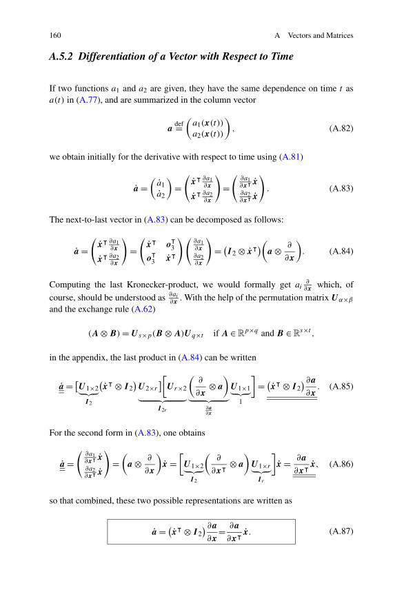
A.5.2 Differentiation of a Vector with Respect to Time
If two functions a1 and a2 are given, they have the same dependence on time t asa(t) in (A.77), and are summarized in the column vector
adef=
(a1(x(t))
a2(x(t))
), (A.82)
we obtain initially for the derivative with respect to time using (A.81)
a =(
a1a2
)=
(xᵀ ∂a1
∂x
xᵀ ∂a2∂x
)=
(∂a1∂xᵀ x∂a2∂xᵀ x
). (A.83)
The next-to-last vector in (A.83) can be decomposed as follows:
a =(
xᵀ ∂a1∂x
xᵀ ∂a2∂x
)=
(xᵀ o
ᵀ3
oᵀ3 xᵀ
)(∂a1∂x∂a2∂x
)= (
I 2 ⊗ xᵀ)(a ⊗ ∂
∂x
). (A.84)
Computing the last Kronecker-product, we would formally get ai∂∂x which, of
course, should be understood as ∂ai
∂x . With the help of the permutation matrix Uα×β
and the exchange rule (A.62)
(A ⊗ B) = U s×p(B ⊗ A)Uq×t if A ∈ Rp×q and B ∈R
s×t ,
in the appendix, the last product in (A.84) can be written
a = [U1×2︸ ︷︷ ︸
I 2
(xᵀ ⊗ I 2
)U2×r
][U r×2
︸ ︷︷ ︸I 2r
(∂
∂x⊗ a
)
︸ ︷︷ ︸∂a∂x
U1×1︸ ︷︷ ︸1
]= (
xᵀ ⊗ I 2) ∂a
∂x. (A.85)
For the second form in (A.83), one obtains
a =(
∂a1∂xᵀ x∂a2∂xᵀ x
)=
(a ⊗ ∂
∂x
)x =
[U1×2︸ ︷︷ ︸
I 2
(∂
∂xᵀ ⊗ a
)U1×r︸ ︷︷ ︸
I r
]x = ∂a
∂xᵀ x, (A.86)
so that combined, these two possible representations are written as
a = (xᵀ ⊗ I 2
) ∂a
∂x= ∂a
∂xᵀ x. (A.87)
A.5 Differentiation with Respect to Time 161
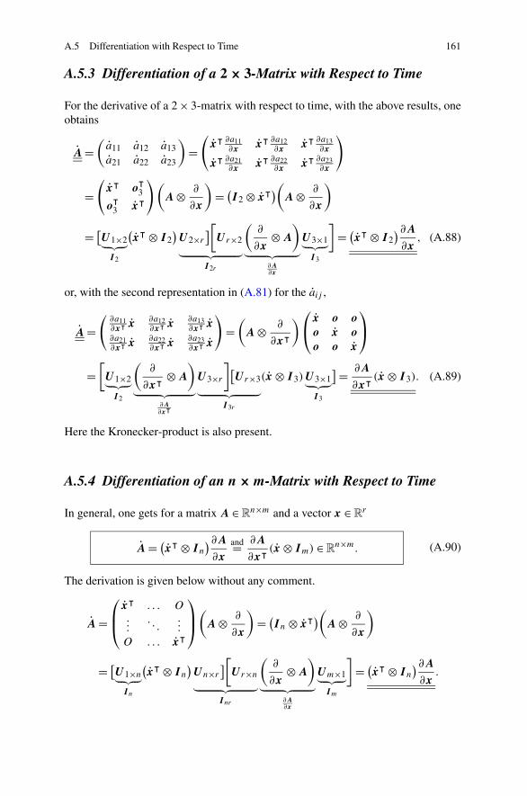
A.5.3 Differentiation of a 2 × 3-Matrix with Respect to Time
For the derivative of a 2 × 3-matrix with respect to time, with the above results, oneobtains
A =(
a11 a12 a13a21 a22 a23
)=
(xᵀ ∂a11
∂x xᵀ ∂a12∂x xᵀ ∂a13
∂x
xᵀ ∂a21∂x xᵀ ∂a22
∂x xᵀ ∂a23∂x
)
=(
xᵀ oᵀ3
oᵀ3 xᵀ
)(A ⊗ ∂
∂x
)= (
I 2 ⊗ xᵀ)(A ⊗ ∂
∂x
)
= [U1×2︸ ︷︷ ︸
I 2
(xᵀ ⊗ I 2
)U2×r
][U r×2
︸ ︷︷ ︸I 2r
(∂
∂x⊗ A
)
︸ ︷︷ ︸∂A∂x
U3×1︸ ︷︷ ︸I 3
]= (
xᵀ ⊗ I 2)∂A
∂x, (A.88)
or, with the second representation in (A.81) for the aij ,
A =(
∂a11∂xᵀ x ∂a12
∂xᵀ x ∂a13∂xᵀ x
∂a21∂xᵀ x ∂a22
∂xᵀ x ∂a23∂xᵀ x
)=
(A ⊗ ∂
∂xᵀ
)⎛⎝
x o o
o x o
o o x
⎞⎠
=[U1×2︸ ︷︷ ︸
I 2
(∂
∂xᵀ ⊗ A
)
︸ ︷︷ ︸∂A∂xᵀ
U3×r
][U r×3
︸ ︷︷ ︸I 3r
(x ⊗ I 3)U3×1︸ ︷︷ ︸I 3
] = ∂A
∂xᵀ (x ⊗ I 3). (A.89)
Here the Kronecker-product is also present.
A.5.4 Differentiation of an n × m-Matrix with Respect to Time
In general, one gets for a matrix A ∈Rn×m and a vector x ∈ R
r
A = (xᵀ ⊗ In
)∂A
∂x
and= ∂A
∂xᵀ (x ⊗ Im) ∈Rn×m. (A.90)
The derivation is given below without any comment.
A =⎛⎜⎝
xᵀ . . . O...
. . ....
O . . . xᵀ
⎞⎟⎠
(A ⊗ ∂
∂x
)= (
In ⊗ xᵀ)(A ⊗ ∂
∂x
)
= [U1×n︸ ︷︷ ︸
In
(xᵀ ⊗ In
)Un×r
][U r×n
︸ ︷︷ ︸Inr
(∂
∂x⊗ A
)
︸ ︷︷ ︸∂A∂x
Um×1︸ ︷︷ ︸Im
]= (
xᵀ ⊗ In
)∂A
∂x.
162 A Vectors and Matrices
A =(
A ⊗ ∂
∂xᵀ
)⎛⎜⎝
x . . . O...
. . ....
O . . . x
⎞⎟⎠ =
(A ⊗ ∂
∂xᵀ
)(In ⊗ x)
=[U1×n︸ ︷︷ ︸
In
(∂
∂xᵀ ⊗ A
)
︸ ︷︷ ︸∂A∂xᵀ
Um×r
][U r×m
︸ ︷︷ ︸Imr
(x ⊗ Im)Um×1] = ∂A
∂xᵀ (x ⊗ In).
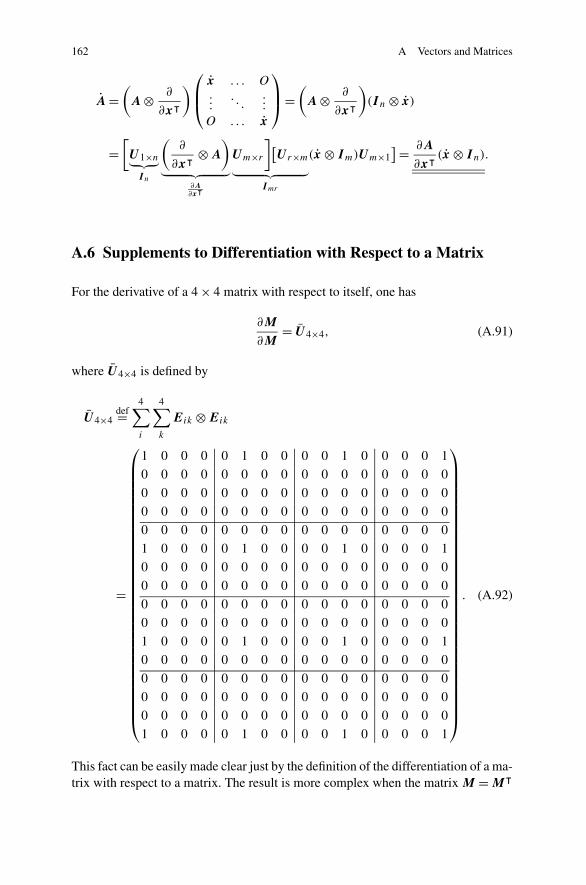
A.6 Supplements to Differentiation with Respect to a Matrix
For the derivative of a 4 × 4 matrix with respect to itself, one has
∂M
∂M= U4×4, (A.91)
where U4×4 is defined by
U4×4def=
4∑i
4∑k
Eik ⊗ Eik
=
⎛⎜⎜⎜⎜⎜⎜⎜⎜⎜⎜⎜⎜⎜⎜⎜⎜⎜⎜⎜⎜⎜⎜⎜⎜⎜⎜⎜⎜⎜⎜⎜⎝
1 0 0 0 0 1 0 0 0 0 1 0 0 0 0 1
0 0 0 0 0 0 0 0 0 0 0 0 0 0 0 0
0 0 0 0 0 0 0 0 0 0 0 0 0 0 0 0
0 0 0 0 0 0 0 0 0 0 0 0 0 0 0 0
0 0 0 0 0 0 0 0 0 0 0 0 0 0 0 0
1 0 0 0 0 1 0 0 0 0 1 0 0 0 0 1
0 0 0 0 0 0 0 0 0 0 0 0 0 0 0 0
0 0 0 0 0 0 0 0 0 0 0 0 0 0 0 0
0 0 0 0 0 0 0 0 0 0 0 0 0 0 0 0
0 0 0 0 0 0 0 0 0 0 0 0 0 0 0 0
1 0 0 0 0 1 0 0 0 0 1 0 0 0 0 1
0 0 0 0 0 0 0 0 0 0 0 0 0 0 0 0
0 0 0 0 0 0 0 0 0 0 0 0 0 0 0 0
0 0 0 0 0 0 0 0 0 0 0 0 0 0 0 0
0 0 0 0 0 0 0 0 0 0 0 0 0 0 0 0
1 0 0 0 0 1 0 0 0 0 1 0 0 0 0 1
⎞⎟⎟⎟⎟⎟⎟⎟⎟⎟⎟⎟⎟⎟⎟⎟⎟⎟⎟⎟⎟⎟⎟⎟⎟⎟⎟⎟⎟⎟⎟⎟⎠
. (A.92)
This fact can be easily made clear just by the definition of the differentiation of a ma-trix with respect to a matrix. The result is more complex when the matrix M = Mᵀ
A.6 Supplements to Differentiation with Respect to a Matrix 163
From a sheet of letter paper, one can form a cylinder or a cone, but it is impossibleto obtain a surface element of a sphere without folding, stretching or cutting. Thereason lies in the geometry of the spherical surface: No part of such a surface canbe isometrically mapped onto the plane.
B.1 Curvature of a Curved Line in Three Dimensions
In a plane, the tangent vector remains constant when one moves on it: the plane hasno curvature. The same is true for a straight line when the tangent vector coincideswith the line. If a line in a neighbourhood of one of its points is not a straight line, itis called a curved line. The same is valid for a curved surface. We consider curves inthe three-dimensional space with the position vector x(q) of points parametrized bythe length q . The direction of a curve C at the point x(q) is given by the normalizedtangent vector
t(q)def= x′(q)
‖x′(q)‖ ,
with x′(q)def= ∂x(q)
∂q. Passing through a curve from a starting point x(q0) to an end-
point x(q) does not change the tangent vector t in a straight line, the tip of thetangent vector does not move, thus describing a curve of length 0. If the curve iscurved, then the tip of the tangent vector describes an arc of length not equal tozero. As arc length we call the integral over a curved arc with endpoints q0 and q
(q > q0):∫ q
q0
+√
x′21 + x′2
2 + x′23 dq =
∫ q
q0
+√x′ᵀx′ dq =
∫ q
q0
∥∥x′∥∥dq. (B.1)
This formula arises as follows: Suppose the interval [q0, q] is divided by the pointsq0 < q1 < · · · < qn = q , then the length σn of the inscribed polygon in the curve
(B.2)By the mean value theorem of differential calculus, for every smooth curve betweenqk and qk+1 there exists a point q
(i)k such that
xi(qk) − xi(qk+1) = x′i
(q
(i)k
)(qk+1 − qk) (B.3)
for i = 1,2 and 3. Inserting (B.3) into (B.2) yields
σn =n∑
k=0
[qk+1 − qk]√[
x′1
(q
(1)k
)]2 + [x′
2
(q
(2)k
)]2 + [x′
3
(q
(3)k
)]2. (B.4)
From (B.4) one gets, as qk+1 − qk → 0, (B.1).A measure of the curvature of a curve is the rate of change of the direction. The
curvature is larger when the change of direction of the tangent vector t is greater.Generally, we therefore define as a curvature of a curve C at a point x(q0)
κ(q0)def= lim
q→q0
length of t
length of x= ‖t ′(q0)‖
‖x′(q0)‖ , (B.5)
where
length of tdef=
∫ q
q0
∥∥t ′∥∥dq
and
length of xdef=
∫ q
q0
∥∥x′∥∥dq.
A straight line has zero curvature. In the case of a circle, the curvature is con-stant; the curvature is greater, the smaller the radius. The reciprocal value 1/κ of thecurvature is called the curvature radius.
B.2 Curvature of a Surface in Three Dimensions
B.2.1 Vectors in the Tangent Plane
Already in the nineteenth century, Gauss investigated how from the measurementson a surface one can make conclusions about its spatial form. He then came to hismain result, the Theorema Egregium, which states that the Gaussian curvature of a
B.2 Curvature of a Surface in Three Dimensions 167
surface depends only on the internal variables gij and their derivatives. This resultis deduced in the following.
Suppose an area is defined as a function x(q1, q2) ∈ R3 of the two coordinates
q1 and q2. At a point P of the surface, the tangent plane is, for example, spanned by
the two tangent vectors x1def= ∂x
∂q1and x2
def= ∂x∂q2
. If the two tangent vectors x1 andx2 are linearly independent, any vector in the tangent plane can be decomposed ina linear combination of the two vectors, e.g. as
v1x1 + v2x2.
The scalar product of two vectors from the tangent plane is then defined as
(v · w)def= (
v1xᵀ1 + v2x
ᵀ2
)(w1x1 + w2x2
)
= vᵀ
⎛⎝
xᵀ1
xᵀ2
⎞⎠ [x1,x2]w = vᵀ
⎛⎝
xᵀ1 x1 x
ᵀ1 x2
xᵀ2 x1 x
ᵀ2 x2
⎞⎠w = vᵀGw.
As xᵀ1 x2 = x
ᵀ2 x1, the matrix Gᵀ = G is symmetric. In addition, one has
‖v‖ = √(v · v) = √
vᵀGv.
Now we want to define the curvature by oriented parallelograms. Let v ∧ w be theoriented parallelogram defined by the vectors v and w in that order. w∧v = −v∧wis then the parallelogram with the opposite orientation, area(w∧v) = −area(v∧w).The determinant of the matrix G is then obtained as
On the other hand, one has ‖x1 × x2‖ = ‖x1‖ · ‖x2‖ · sinΘ , and so
‖x1 × x2‖ = √g = area(x1 ∧ x2). (B.6)
For the vector product of two vectors v and w from the tangent plane, one gets, onthe other hand,
(v1x1 + v2x2
) × (w1x1 + w2x2
)
= v1w1 (x1 × x1)︸ ︷︷ ︸0
+v1w2(x1 × x2) + v2w1 (x2 × x1)︸ ︷︷ ︸−(x1×x2)
+v2w2 (x2 × x2)︸ ︷︷ ︸0
= (v1w2 − v2w1)
︸ ︷︷ ︸def=detR
(x1 × x2),
168 B Some Differential Geometry
or
area(v ∧ w) = detR · area(x1 ∧ x2),
so
area(v ∧ w) = detR√
g. (B.7)
The area of the parallelogram spanned by two vectors in the tangential surface isthus determined by the vector components and the surface defining the matrix G.
B.2.2 Curvature and Normal Vectors
For two-dimensional surfaces, one should define the curvature at a point withoutusing the tangent vectors directly because there are infinitely many of them in thetangent plane. However, any smooth surface in R
3 has at each point a unique normaldirection, which is one-dimensional, so it can be described by the unit normal vector.A normal vector at x(q) is defined as the normalized vector perpendicular to thetangent plane:
n(q)def= x1 × x2
‖x1 × x2‖ .
If the surface is curved, the normal vector changes with displacement according to
ni (q)def= ∂n(q)
∂qi.
These change vectors ni lie in the tangent plane because
∂(n · n)
∂qi= 0 =
(∂n
∂qi· n
)+
(n · ∂n
∂qi
)= 2(ni · n).
The bigger the area spanned by the two change vectors n1 and n2 lying in the tangentplane, the bigger the curvature at the considered point. If Ω is an area of the tangentsurface which contains the point under consideration, then the following curvaturedefinition is obvious:
κ(q)def= lim
Ω→q
area of n(Ω)
area of Ω= lim
Ω→q
∫∫Ω
‖n1(q) × n2(q)‖dq1 dq2∫∫
Ω‖x1(q) × x2(q)‖dq1 dq2
= ‖n1(q) × n2(q)‖‖x1(q) × x2(q)‖ = area of n1(q) ∧ n2(q)
area of x1(q) ∧ x2(q). (B.8)
Since both n1 and n2 lie in the tangent plane, they can be displayed as linear com-binations of the vectors x1 and x2:
n1 = −b11x1 − b2
1x2 and n2 = −b12x1 − b2
2x2. (B.9)
B.2 Curvature of a Surface in Three Dimensions 169
Combining together the coefficients −bji in the matrix B , this corresponds to the
matrix R in (B.7), and (B.6) then yields the Gauss-curvature
κ(q) = detB. (B.10)
To confirm the Theorema Egregium of Gauss, one must now shown that B dependsonly on the inner values gij and their derivatives!
B.2.3 Theorema Egregium and the Inner Values gij
First, we examine the changes of the tangent vectors xk by looking at their deriva-tives
xjkdef= ∂xk
∂qj= ∂2x
∂qj ∂qk, (B.11)
which implies that
xjk = xkj . (B.12)
Since the two vectors x1 and x2 are a basis for the tangent plane and the vector n isorthonormal to this plane, any vector in R
3, including the vector xjk , can assembledas a linear combination of these three vectors:
xjk = Γ 1jkx1 + Γ 2
jkx2 + bjkn. (B.13)
The vectors xjk can be summarized in a 4 × 2-matrix as follows:
∂2x
∂q∂qᵀ =(
x11 x12x21 x22
)= Γ 1 ⊗ x1 + Γ 2 ⊗ x2 + B ⊗ n, (B.14)
where
Γ idef=
(Γ i
11 Γ i12
Γ i21 Γ i
22
)
and
Bdef=
(b11 b12b21 b22
).
Multiplying (B.14) from the left by the matrix (I 2 ⊗ nᵀ), due to nᵀxi = 0 and(I 2 ⊗ nᵀ)(B ⊗ n) = B ⊗ (nᵀn) = B ⊗ 1 = B , one finally obtains
B = (I 2 ⊗ nᵀ) ∂2x
∂q∂qᵀ =(
nᵀx11 nᵀx12nᵀx21 nᵀx22
), (B.15)
170 B Some Differential Geometry
i.e. the 2 × 2-matrix B is symmetric. This matrix is called the Second Fundamen-tal Form of the surface. The First Quadratic Fundamental Form is given by theconnection
G = ∂xᵀ
∂q· ∂x
∂qᵀ , (B.16)
or more precisely, by the right-hand side of the equation for the squared line elementds of the surface:
ds2 = dqᵀ Gdq.
Gauss designates, as is still in elementary geometry today, the elements of the matrixG in this way:
G =(
E F
F G
).
While G therefore plays a critical role in determining the length of a curve in an area,B is, as we will see later, decisively involved in the determination of the curvatureof a surface. A further representation of the matrix B is obtained from the derivativeof the scalar product of the mutually orthogonal vectors n and xi :
nᵀ ∂x
∂qᵀ = 0ᵀ;
because this derivative is, according to (A.73),
∂
∂q
(nᵀ ∂x
∂qᵀ
)= ∂nᵀ
∂q· ∂x
∂qᵀ + (I 2 ⊗ nᵀ) ∂2x
∂q∂qᵀ = 02×2.
With (B.15) we obtain
B = −∂nᵀ
∂q· ∂x
∂qᵀ , (B.17)
i.e. a further interesting form for the matrix B
B = −(
nᵀ1 x1 n
ᵀ1 x2
nᵀ2 x1 n
ᵀ2 x2
). (B.18)
The two equations (B.9) can be summarized to a matrix equation as follows:
[n1|n2] = ∂n
∂qᵀ = ∂x
∂qᵀ
(−b1
1 −b12
−b21 −b2
2
)= ∂x
∂qᵀ · B. (B.19)
This used in (B.18) together with (B.16) yields
B = −Bᵀ · ∂xᵀ
∂q· ∂x
∂qᵀ = −BᵀG,
B.2 Curvature of a Surface in Three Dimensions 171
or transposed
B = −GB, (B.20)
since B and G are both symmetric matrices. Our goal remains to show that theGaussian curvature depends only on the gij ’s and their derivatives with respect toqk , i.e., according to (B.10), one must show that for the matrix B
κ(q) = detB
is valid. We first examine the matrix G. For this purpose, its elements are differen-tiated:
∂gij
∂qk
= xᵀikxj + x
ᵀjkxi .
With (B.13) we obtain
xᵀj xik = Γ 1
ikxᵀj x1 + Γ 2
ikxᵀj x2 + bikx
ᵀj n
= Γ 1ikgj1 + Γ 2
ikgj2.
If we define
Γjik
def= Γ 1ikgj1 + Γ 2
ikgj2
and assemble all four components into a matrix Γ j , we obtain
(Γ 1
j1 Γ 2j1
Γ 1j2 Γ 2
j2
)=
(Γ 1
j1 Γ 2j1
Γ 1j2 Γ 2
j2
)(g11 g12g21 g22
)= Γ jG
ᵀ (B.21)
or, because of Gᵀ = G,
Γ j = Γ jG. (B.22)
It is therefore true that
∂gij
∂qk
= Γjik + Γ i
jk. (B.23)
With the following expression of three different derivatives, one obtains
∂gij
∂qk
+ ∂gik
∂qj
− ∂gjk
∂qi
= Γjik + Γ i
jk + Γ kij + Γ i
jk − Γjik − Γ k
ji , (B.24)
so
Γ ijk = 1
2
(∂gij
∂qk
+ ∂gik
∂qj
− ∂gjk
∂qi
). (B.25)
172 B Some Differential Geometry
Multiplying (B.22) from the right with
G−1 def=(
g[−1]11 g
[−1]12
g[−1]21 g
[−1]22
),
one gets the relation
Γ j = Γ jG−1, (B.26)
i.e. element by element
Γ �jk = 1
2
∑i
g[−1]i� Γ i
jk, (B.27)
so with (B.25)
Γ �jk = 1
2
∑i
g[−1]i�
(∂gij
∂qk
+ ∂gik
∂qj
− ∂gjk
∂qi
). (B.28)
This clarifies the relationship of the Christoffel-symbols Γ �jk with the gij and their
derivatives. Now the direct relationship of these variables with the Gaussian curva-ture κ has to be made. One gets this finally by repeated differentiation of xjk withrespect to q�:
xjk�def= ∂xjk
∂q�=
∑i
∂Γ ijk
∂q�xi +
∑i
Γ ij�xi� + ∂bjk
∂q�n + bjkn�
=∑
i
(∂Γ i
jk
∂q�+ Γ i
j�Γip� − bjkb
i�
)xi +
(∂bjk
∂q�+
∑p
Γpjkbp�
)n. (B.29)
Interchanging in (B.29) k and �, we obtain
xj�k =∑
i
(∂Γ i
j�
∂qk+ Γ i
jkΓipk − bj�b
ik
)xi +
(∂bj�
∂qk+
∑p
Γpj�bpk
)n. (B.30)
Subtracting the two third-order derivatives, we obtain
0 = xj�k − xjk� =∑
i
[Ri�
jk − (bj�b
ik − bjkb
i�
)]xi + (· · · )n, (B.31)
with
Ri�jk
def= ∂Γ ij�
∂qk− ∂Γ i
jk
∂q�+
∑p
Γp
j�Γip� −
∑p
ΓpjkΓ
ipk. (B.32)
B.2 Curvature of a Surface in Three Dimensions 173
Since the vectors x1,x2 and n are linearly independent, the square bracket in (B.31)must be zero, which implies
Ri�jk = bj�b
ik − bjkb
i�. (B.33)
Defining
Ri�jk =
∑i
gihRi�jk, (B.34)
one gets
Ri�jk = g1hbj�b
1k − g1hbjkb
1� + g2hbj�b
2k − g2hbjkb
2� = bj�bkh − bjkb�h. (B.35)
In particular,
R1212 = b22b11 − b21b21 = detB. (B.36)
It is therefore true that
κ(q) = det B = detB
detG= R12
12
g,
κ(q) = R1212
g, (B.37)
which has finally proved the Theorema Egregium because, due to (B.34), Ri�jk de-
pends on Ri�jk ; according to (B.32), Ri�
jk only depends on Γ kij and their derivatives
and, in accordance with (B.25), the Γ kij ’s depend only on the gik’s and their deriva-
tives. In the form
κ(q) = detB
detG, (B.38)
the paramount importance of the two fundamental forms is expressed.
Remarks
1. Euclidean geometry of is based on a number of Axioms that require no proofs.One is the parallel postulate stating that to every line one can draw through apoint not belonging to it one and only one other line which lies in the same planeand does not intersect the former line. This axiom is replaced in the hyperbolicgeometry in that it admits infinitely many parallels. An example is the surfaceof a hyperboloid. In the elliptical geometry, for example, on the surface of anellipsoid and, as a special case, on a spherical surface, there are absolutely noparallels because all great circles, which are here the “straight lines”, meet in
174 B Some Differential Geometry
two points. In Euclidean geometry, the distance between two points with theCartesian coordinates x1, x2, x3 and x1 + dx1, x2 + dx2, x3 + dx3 is simply
ds =√
dx21 + dx2
2 + dx23 ,
and in the other two geometries this formula is replaced by
ds2 = a1 dx21 + a2 dx2
2 + a3 dx23 ,
where the coefficients ai are certain simple functions of xi , in the hyperboliccase, of course, different than in the elliptic case. A convenient analytical repre-sentation of curved surfaces is the above used Gaussian parameter representationx = x(q1, q2), where Gauss attaches as curved element:
ds2 = E dq21 + 2F dq1 dq2 + Gdq2
2 .
As an example, we introduce the Gauss-specific parameter representation of theunit sphere, with θ = q1 and ϕ = q2:
x1 = sin θ cosϕ, x2 = sin θ sinϕ, x3 = cosϕ.
For the arc element of the unit sphere, we obtain
ds2 = dθ2 + sin2 θ(dϕ)2.
Riemann generalized the Gaussian theory of surfaces, which is valid fortwo-dimensional surfaces in three-dimensional spaces, to p-dimensional hyper-surfaces in n-dimensional spaces, i.e. where
x = x(q1, . . . , qp) ∈ Rn
is a point on the hypersurface. He made in addition the fundamentally importantstep, to set up a homogeneous quadratic function of dqi with arbitrary functionsof the qi as coefficients, as the square of the line elements (quadratic form)
ds2 =∑ik
gik dqi dqk = dqᵀGdq.
.2. The above-occurring Ri�
jk can be used as matrix elements of the 4 × 4-matrix R,the Riemannian Curvature Matrix, to be constructed as a block matrix as follows:
R =(
R11 R12
R21 R22
),
where the 2 × 2 sub-matrices have the form:
Ri� =(
Ri�11 Ri�
12
Ri�21 Ri�
22
).
B.2 Curvature of a Surface in Three Dimensions 175
In particular, R1212 is the element in the top right corner of the matrix R = GR.
3. Expanding the representation of x(q + �q) in a Taylor series, one obtains
x(q + �q) = x(q) +∑
i
xi�qi + 1
2
∑i,k
xik�qi�qk + σ(3).
Subtracting x(q) on both sides of this equation and multiplying the result fromthe left with the transposed normal vector nᵀ, we obtain
nᵀ[x(q + �q) − x(q)
] =∑
i
nᵀxi︸︷︷︸0
�qi + 1
2
∑i,k
nᵀxik︸ ︷︷ ︸bik
�qi�qk + σ(3)
= nᵀ�x(q)def= ��.
Thus
d�≈1
2
∑i,k
bik dqi dqk.
The coefficients of the second fundamental form, i.e. the elements of the ma-trix B , Gauss denotes by L,M and N . Then the distance d� of the pointx(q1 + dq1, q2 + dq2) to the tangent surface at the point x(q1, q2) is
d�≈1
2
(Ldq2
1 + 2M dq1 dq2 + N dq22
).
The normal curvature κ of a surface at a given point P and in a given direction q
is defined as
κdef= Ldq2
1 + 2M dq1 dq2 + N dq22
E dq21 + 2F dq1 dq2 + Gdq2
2
. (B.39)
The so-defined normal curvature depends, in general, on the chosen direc-tion dq . Those directions, in which the normal curvatures at a given point as-sume an extreme value, are named the main directions of the surface at thispoint. As long as we examine real surfaces, the quadratic differential formE dq2
1 + 2F dq1 dq2 + Gdq22 is positive definite, i.e. it is always positive for
dq �= 0. Thus the sign of the curvature depends only on the quadratic differentialform Ldq2
1 + 2M dq1 dq2 + N dq22 in the numerator of (B.39). There are three
cases:
(a) LN − M2 > 0, i.e. B is positive definite, and the numerator retains the samesign, in each direction one is looking. Such a point is called an ellipticalpoint. An example is any point on an ellipsoid, in particular, of course, on asphere.
(b) LN −M2 = 0, i.e. B is semi-definite. The surface behaves at this point as atan elliptical point except in one direction where is κ = 0. This point is calledparabolic. An example is any point on a cylinder.
176 B Some Differential Geometry
(c) LN − M2 < 0, i.e. B is indefinite. The numerator does not keep the samesign for all directions. Such a point is called hyperbolic, or a saddle point.An example is a point on a hyperbolic paraboloid.
Dividing the numerator and the denominator in (B.39) by dq2 and introducing
dq1/dq2def= λ, we obtain
κ(λ) = L + 2Mλ + Nλ2
E + 2Fλ + Gλ2(B.40)
and from this the extreme values from
dκ
dλ= 0
as those satisfying(E + 2Fλ + Gλ2)(M + Nλ) − (
L + 2Mλ + Nλ2)(F + Gλ) = 0. (B.41)
In this case, the resulting expression for κ is
κ = L + 2Mλ + Nλ2
E + 2Fλ + Gλ2= M + Nλ
F + Gλ. (B.42)
Since furthermore
E + 2Fλ + Gλ2 = (E + Fλ) + λ(F + Gλ)
and
L + 2Mλ + Nλ2 = (L + Mλ) + λ(M + Nλ),
(B.40) can be transformed into the simpler form
κ = L + Mλ
E + Fλ. (B.43)
From this the two equations for κ follow:
(κE − L) + (κF − M)λ = 0,
(κF − M) + (κG − N)λ = 0.
These equations are simultaneously satisfied if and only if
det
(κE − L κF − M
κF − M κG − N
)= 0. (B.44)
This can also be written as
det(κG − B) = 0. (B.45)
B.2 Curvature of a Surface in Three Dimensions 177
This is the solvability condition for the eigenvalue equation
κG − B = 0,
which can be transformed into
κI − G−1B = 0. (B.46)
This results in a quadratic equation for κ . The two solutions are called the principalcurvatures and are denoted as κ1 and κ2. The Gaussian curvature κ of a surface at agiven point is the product of the principal curvatures κ1 and κ2 of the surface in thispoint. According to Vieta’s root theorem, the product of the solutions is equal to thedeterminant of the matrix G−1B , so finally,
κ = κ1κ2 = det(G−1B
) = detB
detG= LN − M2
EG − F 2.
Appendix CGeodesic Deviation
Geodesics are the lines of general manifolds along which, for example, free particlesmove. In a flat space the relative velocity of each pair of particles is constant, so thattheir relative acceleration is always equal to zero. Generally, due to the curvature ofspace, the relative acceleration is not equal to zero.
The curvature of a surface can be illustrated as follows [21]. Suppose there aretwo ants on an apple which leave a starting line at the same time and follow withthe same speed geodesics which are initially perpendicular to the start line. Initially,their paths are parallel, but, due to the curvature of the apple, they are approachingeach other from the beginning. Their distance ξ from one another is not constant,i.e., in general, the relative acceleration of the ants moving on geodesics with con-stant velocity is not equal zero if the area over which they move is curved. So thecurvature can be indirectly perceived through the so-called geodesic deviation ξ .
The two neighboring geodesics x(u) and x(u) have the distance
ξ(u)def= x(u) − x(u), (C.1)
where u is the proper time or distance.The mathematical descriptions of these geodesics are
¨x + (I 4 ⊗ ˙xᵀ)
Γ ˙x = 0, (C.2)
x + (I 4 ⊗ xᵀ)
Γ x = 0. (C.3)
The Christoffel-matrix Γ is approximated by
Γ ≈ Γ + ∂Γ
∂xᵀ (ξ ⊗ I 4). (C.4)
Subtracting (C.3) from (C.2) and considering (C.1) and (C.4), one obtains
With ˙x = ξ + x and neglecting quadratic and higher powers of ξ and ξ , one obtainsfrom (C.5)
ξ + (I 4 ⊗ ξ
ᵀ)Γ x + (
I 4 ⊗ xᵀ)Γ ξ + (
I 4 ⊗ xᵀ) ∂Γ
∂xᵀ (ξ ⊗ I 4)x = 0. (C.6)
Hence
Dξ
du= ξ + (
I 4 ⊗ ξᵀ)Γ x (C.7)
and
D2ξ
du2= D
du
(ξ + (
I 4 ⊗ ξᵀ)Γ x
)
= ξ + d
du
{(I 4 ⊗ ξᵀ
)Γ x
} + (I 4 ⊗ [
ξ + (I 4 ⊗ ξᵀ
)Γ x
]ᵀ)Γ x
= ξ + d
du
{(I 4 ⊗ ξᵀ
)Γ x
} + (I 4 ⊗ ξ
ᵀ)Γ x + (
I 4 ⊗ [(I 4 ⊗ ξᵀ
)Γ x
]ᵀ)Γ x.
(C.8)
For the second term, by (C.3), one gets
d
du
{(I 4 ⊗ ξᵀ
)Γ x
} = (I 4 ⊗ ξ
ᵀ)Γ x + (
I 4 ⊗ ξᵀ) ∂Γ
∂xᵀ (x ⊗ I 4)x + (I 4 ⊗ ξᵀ
)Γ x
= (I 4 ⊗ ξ
ᵀ)Γ x + (
I 4 ⊗ ξᵀ) ∂Γ
∂xᵀ (x ⊗ I 4)x
− (I 4 ⊗ ξᵀ
)Γ
(I 4 ⊗ xᵀ)
Γ x. (C.9)
Equation (C.9) used in (C.8) yields
D2ξ
du2= ξ + (
I 4 ⊗ ξᵀ)
Γ x + (I 4 ⊗ ξᵀ
) ∂Γ
∂xᵀ (x ⊗ I 4)x − (I 4 ⊗ ξᵀ
)Γ
(I 4 ⊗ xᵀ)
Γ x
+ (I 4 ⊗ ξ
ᵀ)Γ x + (
I 4 ⊗ [(I 4 ⊗ ξᵀ
)Γ x
]ᵀ)Γ x. (C.10)
Remark Since the sub-matrices Γ i are symmetric, it is generally true that(I 4 ⊗ aᵀ)
Γ b = (I 4 ⊗ bᵀ
)Γ a. (C.11)
In addition, one has (I 4 ⊗ aᵀ)Γ b = Γ (I 4 ⊗ a)b = Γ (b ⊗ a) and (I 4 ⊗ bᵀ)Γ a =Γ (I 4 ⊗ b)a = Γ (a ⊗ b), thus, due to (C.11),
Γ (b ⊗ a) = Γ (a ⊗ b). (C.12)
With (C.11), one has from (C.10)
ξ + (I 4 ⊗ ξ
ᵀ)Γ x + (
I 4 ⊗ xᵀ)Γ ξ
C Geodesic Deviation 181
= D2ξ
du2− (
I 4 ⊗ ξᵀ) ∂Γ
∂xᵀ (x ⊗ I 4)x
+ (I 4 ⊗ ξᵀ
)Γ
(I 4 ⊗ xᵀ)
Γ x − (I 4 ⊗ [(
I 4 ⊗ ξᵀ)Γ x
]ᵀ)Γ x. (C.13)
For (I 4 ⊗ ξᵀ)Γ (I 4 ⊗ xᵀ)Γ x one can write
(I 4 ⊗ ξᵀ
)Γ
(I 4 ⊗ xᵀ)
Γ x = (I 4 ⊗ ξᵀ
)Γ Γ (I 4 ⊗ x)x, (C.14)
and the expression (I 4 ⊗ [(I 4 ⊗ ξᵀ)Γ x]ᵀ)Γ x can be rewritten as
(I 4 ⊗ [(
I 4 ⊗ ξᵀ)Γ x
]ᵀ)Γ x
= Γ(I 4 ⊗ (
I 4 ⊗ ξᵀ)Γ x
)x
= Γ(I 16 ⊗ ξᵀ
)(I 4 ⊗ Γ x)x = (
I 4 ⊗ ξᵀ)(Γ ⊗ I 4)(I 4 ⊗ Γ )(I 4 ⊗ x)x. (C.15)
With (C.14) (in somewhat modified form) and (C.15) one obtains for (C.13)
ξ + (I 4 ⊗ ξ
ᵀ)Γ x + (
I 4 ⊗ xᵀ)Γ ξ
= D2ξ
du2− (
I 4 ⊗ ξᵀ) ∂Γ
∂xᵀ (x ⊗ I 4)x
+ (I 4 ⊗ ξᵀ
)[Γ Γ − (Γ ⊗ I 4)(I 4 ⊗ Γ )
](x ⊗ x). (C.16)
Equation (C.16) used in (C.6) provides
D2ξ
du2= −(
I 4 ⊗ xᵀ) ∂Γ
∂xᵀ (ξ ⊗ I 4)x + (I 4 ⊗ ξᵀ
) ∂Γ
∂xᵀ (x ⊗ I 4)x
+ (I 4 ⊗ ξᵀ
)[Γ Γ − (Γ ⊗ I 4)(I 4 ⊗ Γ )
](x ⊗ x). (C.17)
As the 16 × 16-matrix ∂Γ∂xᵀ is symmetric, the first term of the right-hand side can
transformed as follows:
(I 4 ⊗ xᵀ) ∂Γ
∂xᵀ (ξ ⊗ I 4)x = (I 4 ⊗ xᵀ) ∂Γ
∂xᵀU4×4(I 4 ⊗ ξ)x
= (I 4 ⊗ ξᵀ
) ∂Γ
∂xᵀU4×4(I 4 ⊗ x)x.
This in (C.17) provides
D2ξ
du2= (
I 4 ⊗ ξᵀ)[ ∂Γ
∂xᵀ − ∂Γ
∂xᵀU4×4
](x ⊗ I 4)x
+ (I 4 ⊗ ξᵀ
)[Γ Γ − (Γ ⊗ I 4)(I 4 ⊗ Γ )
](x ⊗ x), (C.18)
182 C Geodesic Deviation
and finally,
D2ξ
du2= (
I 4 ⊗ ξᵀ)[
∂Γ
∂xᵀ (I 16 − U4×4) + (Γ Γ − (Γ ⊗ I 4)(I 4 ⊗ Γ )
)]
︸ ︷︷ ︸−R
(x ⊗ x).
(C.19)Using a slightly modified Riemannian curvature matrix R, we finally obtain for thedynamic behavior of the geodesic deviation
D2ξ
du2+ (
I 4 ⊗ ξᵀ)R(x ⊗ x) = 0. (C.20)
In a flat manifold, i.e. in a gravity-free space one has R ≡ 0 and in Cartesian co-ordinates D/du = d/du so that (C.20) reduces to the equation d2ξ/du2 = 0 whosesolution is the linear relationship ξ(u) = ξ0 ·u+ ξ0. If R �= 0, gravity exists and thesolution of (C.20) is nonlinear, curved.
Appendix DAnother Ricci-Matrix
The Ricci-matrix RRic is now defined as the sum of the sub-matrices on the maindiagonal of R
RRicdef=
3∑ν=0
Rνν . (D.1)
Analogously, we define
RRicdef=
3∑ν=0
Rνν
. (D.2)
From (2.194) it can immediately be read that the Ricci-matrix RRic is symmetricbecause R
γ γαβ = R
γ γβα . It is also true that
R = (G−1 ⊗ I 4
)R,
so
Rγ δ = (g−T
γ ⊗ I 4)R
δ =3∑
ν=0
g[−1]γ ν R
νδ, (D.3)
where g−Tγ is the γ th row of G−1 and R
δis the matrix consisting of the sub-matrices
in the δth block column of R, i.e. the matrix elements are
Rγδαβ =
3∑ν=0
g[−1]γ ν Rνδ
αβ . (D.4)
With the help of (D.3), the Ricci-matrix is obtained as
The curvature scalar R is obtained from the Ricci-matrix by taking the trace
Rdef=
∑α
RRic,αα =∑α
∑γ
∑ν
g[−1]γ ν Rαα
νγ =∑γ
∑ν
g[−1]γ ν RRic,νγ . (D.8)
Conversely, we obtain a corresponding relationship
Rγ δαβ =
3∑ν=0
gγνRνδαβ. (D.9)
From (2.165) it directly follows that
RRic,αβ =3∑
γ=0
(∂
∂xβ
Γ γαγ − ∂
∂xγ
Γγαβ +
3∑ν=0
ΓγβνΓ
νγα −
3∑ν=0
Γ γγ νΓ
ναβ
)(D.10)
and from (2.168)
RRic,αβ =3∑
γ=0
(∂
∂xβ
Γ γαγ − ∂
∂xγ
Γγαβ +
3∑ν=0
Γ ναβΓ ν
γ γ −3∑
ν=0
Γ ναγ Γ ν
γβ
). (D.11)
Symmetry of the Ricci-Matrix RRic Even if R itself is not symmetric, the fromR derived Ricci-matrix RRic is symmetric; this will be shown in the following. Thesymmetry will follow from the components equation (D.10) of the Ricci-matrix.One sees immediately that the second and fourth summands are symmetric in α
and β .The symmetry of the term
∑3γ=0
∂∂xβ
Γγαγ in α and β is not seen directly. This can
be checked using the Laplace-expansion theorem for determinants.1 Developing thedeterminant of G along the γ th row yields
1The sum of the products of all elements of a row (or column) with their adjuncts is equal to thedeterminant’s value.
D Another Ricci-Matrix 185
where Aγβ is the element in the γ th row and βth column of the adjoint of G. If g[−1]βγ
is the (βγ )th element of the inverse of G, then g[−1]βγ = 1
gAγβ , so Aγβ = g g
[−1]βγ .
Thus we obtain∂g
∂gγβ
= Aγβ = g g[−1]βγ ,
or
δg = g g[−1]βγ δgγβ,
or
∂g
∂xα
= g g[−1]βγ
∂gγβ
∂xα
,
i.e.
1
g
∂g
∂xα
= g[−1]βγ
∂gγβ
∂xα
. (D.12)
Using (2.62), on the other hand, one has
3∑γ=0
Γ γαγ =
3∑γ=0
3∑β=0
g[−1]βγ
2
(∂gγβ
∂xα
+ ∂gαβ
∂xγ
− ∂gαγ
∂xβ
),
i.e. the last two summands cancel out and it remains to deal with
3∑γ=0
Γ γαγ =
3∑γ=0
3∑β=0
1
2g
[−1]βγ
∂gγβ
∂xα
.
It follows from (D.12) that
3∑γ=0
∂
∂xβ
Γ γαγ =
3∑γ=0
3∑β=0
1√|g|∂2√|g|∂xα∂xβ
. (D.13)
But this form is immediately seen symmetric in α and β .Now it remains to shown that the third term in (D.10) is symmetric. Its expression
is3∑
γ=0
3∑ν=0
ΓγβνΓ
νγα.
Now one can see that this term is symmetric because
3∑γ,ν=0
ΓγβνΓ
νγα =
3∑γ,ν=0
ΓγνβΓ ν
αγ =3∑
ν,γ=0
Γ νγβΓ γ
αν.
All this shows that the Ricci-matrix RRic is symmetric.
186 D Another Ricci-Matrix
Divergence of the Ricci-Matrix RRic Multiplying the Bianchi-identities (2.199)in the form of
∂
∂xκ
Rνδαβ + ∂
∂xβ
Rνκαδ + ∂
∂xδ
Rνβακ = 0
with gγν and summing over ν, we obtain in P , since there ∂G∂x = 0,
∂
∂xκ
3∑ν=0
gγνRνδαβ + ∂
∂xβ
3∑ν=0
gγνRνκαδ + ∂
∂xδ
3∑ν=0
gγνRνβακ = 0.
Combined with (D.9) this becomes
∂
∂xκ
Rγ δαβ + ∂
∂xβ
Rγ καδ + ∂
∂xδ
Rγβακ = 0. (D.14)
The second term, according to (2.172), may be written as
− ∂
∂xβ
Rγ δακ .
Substituting now γ = δ and summing over γ , one obtains
∂
∂xκ
RRic,αβ − ∂
∂xβ
RRic,ακ +3∑
γ=0
∂
∂xγ
Rγβακ = 0. (D.15)
In the third summand, one can, according to (2.171), replace Rγβακ by −R
αβγ κ . If we
set α = β and sum over α, we obtain for (D.15) with the trace Rdef= ∑3
α=0 RRic,αα
of the Riccati-matrix RRic
∂
∂xκ
R −3∑
α=0
∂
∂xα
RRic,ακ −3∑
γ=0
∂
∂xγ
RRic,γ κ = 0. (D.16)
If in the last sum the summation index γ is replaced by α, we can finally summarize:
∂
∂xκ
R − 23∑
α=0
∂
∂xα
RRic,ακ = 0. (D.17)
One would get the same result, if one were to start with the equation:
∂
∂xκ
Rγ δαβ − 2
∂
∂xβ
Rγ δακ = 0. (D.18)
D Another Ricci-Matrix 187
Indeed, if we set δ = γ and sum over γ , we get first
∂
∂xκ
RRic,αβ − 2∂
∂xβ
RRic,ακ = 0.
If we now set α = β and sum over α, we will again arrive at (D.17).A different result is obtained when starting from (D.18) (with ν instead of γ )
first, multiplying this equation by g[−1]γ ν to get
∂
∂xκ
g[−1]γ ν Rνδ
αβ − 2∂
∂xβ
g[−1]γ ν Rνδ
ακ = 0,
then again setting γ = δ and summing over γ and ν and noting (D.6):
∑γ
∑ν
∂
∂xκ
g[−1]γ ν R
νγαβ − 2
∑γ
∑ν
∂
∂xβ
g[−1]γ ν Rνγ
ακ
= ∂
∂xκ
RRic,αβ − 2∂
∂xβ
RRic,ακ = 0.
If we now take α = η and sum over α, we finally obtain the important relationship
∂
∂xκ
R − 2∑α
∂
∂xα
RRic,ακ = 0. (D.19)
These are the four equations for the four spacetime coordinates x0, . . . , x3.Finally, this overall result can be represented as
�∇ᵀ(
RRic − 1
2RI 4
)= 0ᵀ. (D.20)
References
1. V.I. Arnold, Mathematical Methods of Classical Mechanics (Springer, Berlin, 1978)2. G. Barton, Introduction to the Relativity Principle (Wiley, New York, 1999)3. H. Bondi, Relativity and Common Sense (Dover Publications, Dover, 1986)4. J.W. Brewer, Kronecker products and matrix calculus in system theory. IEEE Trans. Circuits
Syst. 772–781 (1978)5. J.J. Callahan, The Geometry of Spacetime (Springer, Berlin, 2000)6. S. Carrol, Spacetime and Geometry: An Introduction to General Relativity (Addison Wesley,
San Francisco, 2003)7. S. Chandrasekhar, The Mathematical Theory of Black Holes (Clarendron Press, Oxford, 1983)8. I. Ciufolini, J.A. Wheeler, Gravitation and Inertia (Princeton University Press, Princeton,
1995)9. R. D’Inverno, Introducing Einstein’s Relativity (Clarendon Press, New York, 1992)
10. A. Einstein, Relativity, The Special and the General Theory, 2nd edn. (Edit Benei Noaj, 2007)11. A. Föppl, Über einen Kreiselversuch zur Messung der Umdrehungsgeschwindigkeit der Erde.
Sitzungsber. Bayer. Akad. Wiss. 34, 5–28 (1904)12. J. Foster, J.D. Nightingale, A Short Course in General Relativity (Springer, Berlin, 1995)13. R.G. Gass, F.P. Esposito, L.C.R. Wijewardhansa, L. Witten, Detecting event horizons and
stationary surfaces (1998). arXiv:gr-qc/9808055v14. R. Geroch, Relativity from A to B (Chicago University Press, Chicago, 1981)15. O. Gron, S. Hervik, Einstein’s General Theory of Relativity (Springer, New York, 2007)16. O. Gron, A. Naess, Einstein’s Theory (Springer, New York, 2011)17. J.B. Hartle, Gravity: An Introduction to Einstein’s General Relativity (Addison Wesley, San
Francisco, 2003)18. S.W. Hawking, G.F.R. Ellis, The Large Scale Structure of Space-Time (Cambridge University
Press, Cambridge, 1973)19. I.R. Kenyon, General Relativity (Oxford University Press, Oxford, 1990)20. L.D. Landau, E.M. Lifschitz, Classical Theory of Fields: 2. Course of Theoretical Physics
Series (Butterworth Heinemann, Stoneham, 1987)21. C.W. Misner, K.S. Thorne, J.A. Wheeler, Gravitation (Freeman, San Francisco, 1973)22. R.A. Mould, Basic Relativity (Springer, Berlin, 2002)23. J. Natario, General Relativity Without Calculus (Springer, Berlin, 2011)24. W. Rindler, Essential Relativity (Springer, Berlin, 1977)25. L. Sartori, Understanding Relativity: A Simplified Approach to Einstein’s Theories (University
of California Press, Berkeley, 1996)26. B.F. Schutz, A First Course in General Relativity (Cambridge University Press, Cambridge,
1985)27. H. Stephani, General Relativity (Cambridge University Press, Cambridge, 1977)
28. J. Stewart, Advanced General Relativity (Cambridge University Press, Cambridge, 1991)29. T. Takeuchi, An Illustrated Guide to Relativity (Cambridge University Press, Cambridge,
2010)30. E.F. Taylor, J.A. Wheeler, Spacetime Physics (Freeman, New York, 1992)31. E.F. Taylor, J.A. Wheeler, Black Holes (Addison Wesley, Reading, 2000)32. E.F. Taylor, J.A. Wheeler, Exploring Black Holes: Introduction to General Relativity (Addison
Wesley, San Francisco, 2000)33. M. von Laue, Die Relativitätstheorie. Erster Band: Die spezielle Relativitätstheorie, 7th edn.
(Vieweg, Wiesbaden, 1961)34. R. Wald, General Relativity (Chicago University Press, Chicago, 1984)35. R. Wald, Space, Time and Gravity: Theory of the Big Bang and Black Holes (University Press,
Chicago, 1992)36. S. Weinberg, Gravitation and Cosmology (Wiley, New York, 1972)37. W.J. Wild, A matrix formulation of Einstein’s vacuum field equations, gr-qc/9812095, 31 Dec.