1 APPENDIX Appendix 1. The first appendix presents in an extended fashion the methodology described in short in Section 2 of the main body of the article. 1. The inference function for margins method. Sklar (1959) showed that multivariate distribution can be decomposed into marginal distributions and a dependence function between them. This linking function is called a copula. Formally, let be an n- dimensional distribution function with margins ,…,. Then, there exists a n-copula such that for all in : (1) Under an additional assumption that ,…,are continuous, the copula function is uniquely determined and for any the following relation holds: (2) where is the generalised inverse function for all . The assumption of continuity proves particularly convenient for the estimation of parametric distributions. Let be a sample data matrix, where . If the joint distribution is times differentiable, the density is equal to the product of marginal densities characterised by parameters and the copula density with parameter (Patton (2006)): (3) This implies that the joint log-likelihood is the sum of univariate log-likelihoods and the copula log- likelihood: (4) This form suggests an IFM estimation procedure, consisting of separate estimation of the parameters of marginal distributions and then copula parameter conditionally on marginal distributions’ parameters fixed, rather than a computationally much more involved, though asymptotically efficient joint estimation of parameters for margins and copulas by maximum likelihood (ML). The IFM method was proposed by Joe and Hu (1997) and is commonly applied in similar settings (Patton,
Transcript
1
APPENDIX
Appendix 1.
The first appendix presents in an extended fashion the methodology described in short in
Section 2 of the main body of the article.
1. The inference function for margins method.
Sklar (1959) showed that multivariate distribution can be decomposed into marginal distributions and
a dependence function between them. This linking function is called a copula. Formally, let be an n-
dimensional distribution function with margins ,…, . Then, there exists a n-copula such that for
all in :
(1)
Under an additional assumption that ,…, are continuous, the copula function is uniquely
determined and for any the following relation holds:
(2)
where is the generalised inverse function for all .
The assumption of continuity proves particularly convenient for the estimation of parametric
distributions. Let be a sample data matrix, where . If the joint
distribution is times differentiable, the density is equal to the product of marginal densities
characterised by parameters and the copula density with parameter
(Patton (2006)):
(3)
This implies that the joint log-likelihood is the sum of univariate log-likelihoods and the copula log-
likelihood:
(4)
This form suggests an IFM estimation procedure, consisting of separate estimation of the parameters
of marginal distributions and then copula parameter conditionally on marginal distributions’
parameters fixed, rather than a computationally much more involved, though asymptotically efficient
joint estimation of parameters for margins and copulas by maximum likelihood (ML). The IFM
method was proposed by Joe and Hu (1997) and is commonly applied in similar settings (Patton,
2
2006, Dias and Embrechts, 2010, Christoffersen et al., 2012), primarily because it is computationally
much more effective than the ML method, while the IFM estimator remains asymptotically normal
(see Joe, 1997). The IFM method amounts to first, maximising the likelihood for margins
over -s to obtain transformed variable which is
distributed uniformly on a unit interval, and second, maximising the likelihood of the copula function
over . In our application we use the IFM method and limit ourselves to
two-dimensional distributions, that is dependence between pairs of variables. We use Matlab R2011b,
A. Patton’s Copula Toolbox and J.P. LeSage’s jplv7 toolbox.
1.1. Modelling marginal distributions
Following the IFM method, in the first step we specify parametrically the marginal distributions. To
this end, we need an appropriate family of models. We decide to model the data in a broad tradition of
GARCH framework which captures most of stylised facts observed in financial data (volatility
clustering, asymmetry of gains and losses, thick tails, etc.). In many applications,
a simple GARCH(1,1) model seems to be a reasonable approximation of the underlying process’
dynamics and complex specification search hardly improves forecasting abilities of the model (Hansen
and Lunde, 2001). However, the IFM method requires the marginal distributions to be well-specified
and may be non-robust against misspecifications (Kim et al., 2007). Therefore, the right
implementation of the method involves allowing for a broad family of models from which the right
model will be chosen, as well as using appropriate tests to choose the best alternative from the set of
competing models.
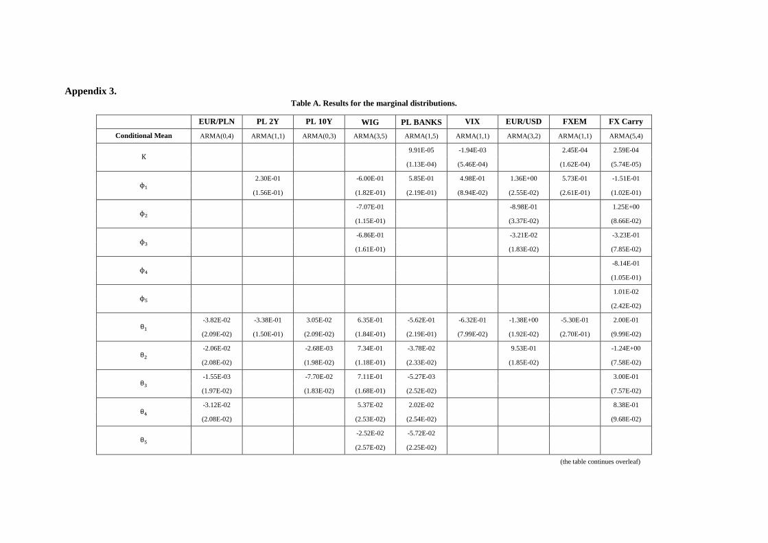
Consider the variable of interest . It is a logarithmic rate of return or a difference depending on the
variable under consideration (e.g. rate of return for currencies, but difference for interest rates). Its
conditional mean is parameterised as ARMA(R,M):
(5)
In the models we consider the maximum possible orders of autoregressive and moving average terms
are low in order to favour more parsimonious representations.
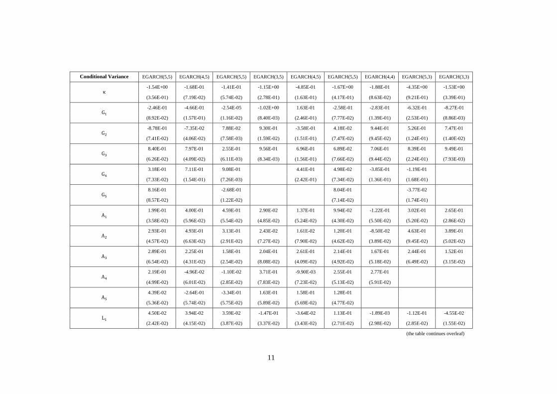
We model the conditional variance of each of the variables either as a pure GARCH(P,Q) or as one of
the asymmetric extensions, EGARCH(P,Q) and GJR(P,Q).
The GARCH(P,Q) model is given as:
(6)
3
with constraints:
The GARCH(P,Q) model is symmetric in that it ignores the sign of the error term. It is now, however,
a well-known phenomenon that financial variables exhibit asymmetries in response to good and bad
news, which traditionally is related to the leverage effect (Black, 1976), or volatility feedback effect
(Campbell and Hentschel, 1992). Thus, an appropriate model should allow for asymmetric news
impact on conditional volatility, i.e. good news ( ) having different effect than bad news
( ). The two important parameterisations are GJR(P,Q) and EGARCH(P,Q). In the GJR(P,Q),
the conditional variance is specified as:
(7)
where if and otherwise, with constraints:
The conditional variance in the EGARCH(P,Q) parameterisation is given by:
(8)
We restrain the maximum orders of P and Q, analogous to the conditional mean specification. Finally,
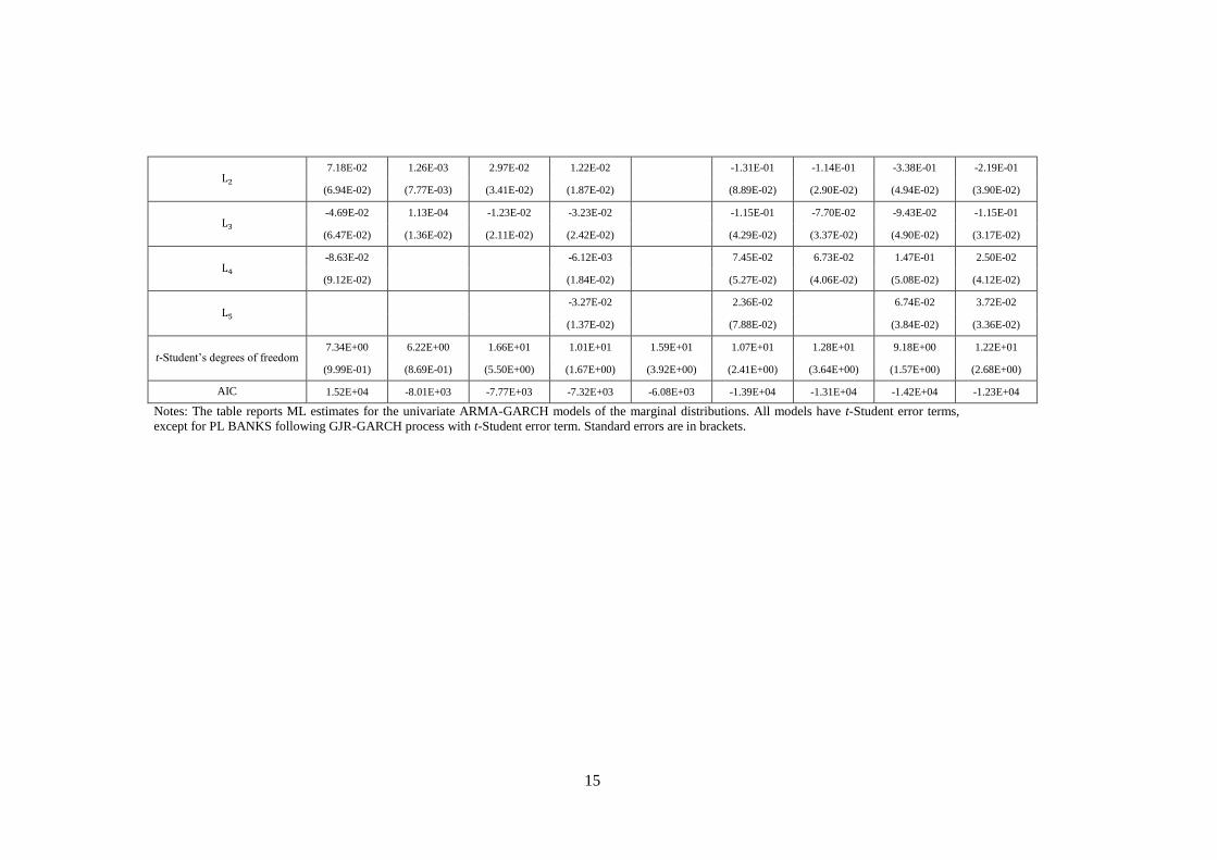
we allow the error term in each of the models to follow either normal or t-Student distribution. The
models are fitted using standard quasi-maximum likelihood estimation (QMLE) method.
A significant advantage of using the IFM method is that the specifications of margins can be tested
using standard diagnostics to ensure that they fit the data well. In the post-estimation analysis, we
employ Ljung-Box test for autocorrelation of the standardised residuals and Engle’s ARCH test for the
presence of the remaining ARCH effects in the residuals . We also employ the Berkowitz (2001)
4
procedure to test if the hypothetical model’s probability integral transform produces observations
which are independently and identically distributed .
Finally, using the conditional cumulative distribution function of the selected model, we transform our
variable of interest into a distributed variable which serves as an input for the second step of
the IFM method. In doing this, we calculate
(9)
which we call transformed variable, where is the information set available at time
comprising past realisations of the variable of interest and is the estimated vector of parameters.
1.2. Modelling the dependence structure
The second stage of the IFM method consists of exploring the sole dependence between the two
random variables using copula functions.
We chose a set of standard, static, parametric functions, most popular in the literature. They allow a
wide range of dependence relations, including asymmetric tail dependence particularly important for
investigating contagion effect. Thus, relations ranging from complete independence to dependence of
differing grade, also in stress times, can be modelled.
The definition of contagion which we employ in the present paper can be operationalised with the so-
called asymptotic tail dependence coefficients introduced by Sibuya (1960) (hereinafter TDC), which,
thus, become our measure of contagion. The coefficients describe the propensity of markets to crash or
boom together, i.e. they measure the dependence between extreme outcomes of the variables. The
upper (lower) TDC is a limiting probability of one variable exceeding (falling behind) a high-order
(low-order) quantile, given that the other variable exceeds (falls behind) the same quantile. Formally,
if is a vector of continuous random variables with marginal distributions and ,
respectively, then the upper and lower TDCs are defined as:
(10)
and:
(11)
If the upper or lower TDC equals zero, the respective extreme values are independent, otherwise we
say that there is dependence between extreme values of the variables considered. Importantly, for the
copulas considered in this paper the TDCs are simple functions of copula parameters. The choice of a
particular copula may in some cases restrict admissible asymptotic dependence (e.g. Gaussian copula
implies asymptotic independence). The Table below gives an overview of the copulas we employ
5
along with their TDCs. Recall that copula functions are defined on a unitary box, ,
where and are distributed as .
Table A. Copula functions and their characteristics.
Copula name
Normal
, where is the bivariate standardised
Gaussian cdf with Pearson’s correlation and is the
inverse of the univariate standardised Gaussian cdf
0
Clayton
0
Rotated
Clayton
,
where is Clayton copula 0
Plackett
, for
,
, for
0
Frank
0
Gumbel exp ,
0
Rotated
Gumbel
,
where is Gumbel copula 0
t-Student
, where is the bivariate t-Student cdf
with parameter and degrees of freedom and is the
inverse of the univariate t-Student cdf with degrees of
freedom
Symmetrised
Joe-Clayton
(SJC)
, where
, for , , and
Independence
copula
0
Having obtained a bi-variate pseudo-sample from any two transformed variables of interest as in eq.
(9), parameters of the above copulas are obtained by maximising the respective likelihood functions.
1.3. Testing copula functions
The IFM procedure amounts to estimating under the assumption that the copula linking marginal
distributions indeed belongs to a chosen family of copulas , i.e. under .
The goodness-of-fit tests, reviewed and compared in Monte Carlo studies by Genest et al. (2009) and
Berg (2009), aim at the complementary issue of testing whether
holds. To our knowledge, the cited papers are the latest available and most comprehensive studies
of such methods in the literature. The experiments are designed to assess, in a number of different
6
setups, the ability of various goodness-of-fit tests to maintain the nominal levels and their power
against a variety of alternatives. The only method that ranks among three best performing in both
power studies is the goodness-of-fit procedure introduced in Genest et al. (2008), ranking first in
Genest et al. (2009) and second in Berg (2009). It is based on the “empirical copula” (a-theoretic
information on the dependence structure, to be defined below), it thus belongs to a class of “blanket
tests” applicable to all copula structures and free of any strategic choices for their use or parameter
fine-tuning. Its implementation involves, however, approximating p-values for testing with a
bootstrap procedure.
The idea is to compare the distance between the “empirical copula” with the estimated parametric one.
To assess whether the distance is significantly different from zero, a bootstrap procedure is
implemented. As the input, the goodness-of-fit test takes the maximally invariant with respect to
continuous, strictly increasing transformations of the components of bivariate distribution statistic, i.e.
ranks obtained from the pseudo-sample . The information on dependence comprised in
the pseudo-sample is summarised in the “empirical copula”
(12)
for , where is obtained by dividing the rank of (in a set ) by , and -
by dividing the respective rank of . The test statistics is based on the empirical process
, and it is given by the Cramer-von Mises statistic
(13)
whose large values imply the rejection of . Asymptotic p-values could in theory be deduced from
the limiting distribution of the above statistic. However, as the asymptotic behaviour of the empirical
process depends on the family of copulas under the composite and on the unknown true parameter
, whose estimate is used in instead, the only viable way to execute statistical test is to resort to
specially adapted parametric bootstrap procedure. It consists of the following steps:
1) Compute and estimate
2) Compute
3) For a large repeat the following for :
a. Generate a random sample from the distribution
b. Using the random sample compute
and estimate
c. Compute
analogously to 2)
4) Approximate p-value with
.
7
The final question, if the above goodness-of-fit test admits more than one copula, concerns the choice
of one particular function for further analysis. We chose the parametric copula with the lowest
distance to the “empirical copula”, as measured by . Then, we compute the TDCs.
8
Appendix 2.
Table A. Definitions of variables and their transformations.
Variable Definition Transformation
EURPLN Nominal spot exchange rate of euro expressed in Polish zloty R
PL2Y 2-year Polish government generic bond yield (%). Currency denomination:
Polish zloty. D
PL10Y 10-year Polish government generic bond yield (%). Currency
denomination: Polish zloty. D
WIG
Warsaw Stock Exchange (WSE) WIG index, total return index which
includes dividends. The index includes all companies listed on the main
market and excludes foreign companies and investment funds. Currency
denomination: Polish zloty.
R
PLBANKS Sub-index of the WIG index which includes 14 banks listed on the WSE R
VIX
CBOE volatility index which reflects a market estimate of future volatility,
based on the weighted average of the implied volatilities for a wide range
of option strikes for the S&P500 index. Commonly used as a market risk-
aversion and uncertainty indicator
R
EURUSD Nominal spot exchange rate of euro expressed in US dollars R
EMCARRY
JPMorgan Income FX index tracking a strategy to generate positive returns
by depositing money in a high yielding currency and borrowing money in a
lower yielding currency, thereby earning the interest rate differential or
“carry”. The strategy analyzes the monthly return generated by an
investment in 14 currency pairs and select the 4 pairs with the highest ratio
of return to risk; and then replicate an equally-weighted trading position in
these 4 currency pairs. Currency of denomination: Euro.
R
EMFX
Morgan Stanley Capital International (MSCI) currency index which sets
the weights of each of 25 currencies equal to the relevant country weight in
the MSCI Emerging Markets equity index (see MSCI). The index
measures total investment performance for included currencies stemming
from appreciation/depreciation against US dollar and from return from
interest earned in holding the currencies.
R
DE2Y 2-year German government generic bond (Bund) yield (%). Currency
denomination: Euro. D
DE10Y 10-year German government generic bond (Bund) yield (%). Currency
denomination: Euro. D
US2Y 2-year US government note yield (%). Currency denomination: US dollar. D
US10Y 10-year US government note yield (%). Currency denomination: US dollar. D
EMBI
Emerging Markets Bond Global Diversified Index measuring the total
return performance of international government bonds issued by emerging
market countries. In order to qualify for index membership, the debt must
be more than one year to maturity and have more than USD 500 million
outstanding inter alia.
D
SP500 Standard and Poor’s index of 500 stocks in US, capitalization-weighted.
Currency denomination: US dollar. R
DAX German total return stock index of 30 stocks with largest capitalization.
Currency denomination: Euro. R
EUBANKS Euro Stoxx Banks index, capitalization-weighted, including 32 EMU
countries banking sector stocks. Currency denomination: Euro. R