Draft Channel Migration Assessment Clallam County 1 December 2011 Appendix D Relative Water Surface Elevation (RWSE) Method Description This is a step-by-step explanation GIS practitioners can use to create a relative surface model. This explanation is geared toward river systems and generating water surface models. The model was originally built under ArcGIS 9.3.2. Definition: A relative surface model is a way by which a user-defined surface can be shown graphically across varying terrain. For example, an inundation map can be created showing which areas on a floodplain (variable surface) are below the flood stage elevation (user-defined surface). Theory The basic theory behind relative surface models is simple. First, a base-surface must be available for the project area. The base surface is most commonly derived from LiDAR. Secondly, a user-defined surface is created. This user-defined surface is commonly a water surface depicting a flood stage, or base flow in a perched river system. The two surfaces are subtracted from one another creating a new “relative” surface with the value “zero” equal to the user-defined surface elevation. As a result, it is easy for the user to graphically display those areas above the user-defined surface (positive numbers) in one color gradation and those areas below (negative numbers) in a different color gradation. This can be used to show flood inundation areas, perched floodplains, cut and fill areas in a grade plan, or any other comparison between two surfaces. Where the theory becomes more complex is during the user-defined surface creation. It is not practical to manually populate an entire grid with specified elevations. Also, in the case of water surfaces, the user-defined surface should be relatively flat. A series of 3-D cross sections is the best approximation method from which the user-defined surface can be created in a river system. In the simplest scenario, the river would run perfectly straight, parallel to the valley it occupies. As a result, all cross sections would be perpendicular to both the river and the valley, and the user-defined surface would be relatively flat across the entire floodplain. Because rivers have meanders and often do not flow either straight or parallel to the valley, a compromise must be made. The compromise is that cross sections should be drawn both perpendicular to the valley and perpendicular to the channel. To do this, the cross sections often end up with kinks or bends in them. The fewer the kinks the better, but drawing a cross section that is perpendicular to the channel and perpendicular to the valley is key. Depending on the water surface being modeled, the cross sections should be drawn roughly perpendicular to the dominant flow vector. Sometimes the high flow vectors are much more uniform in their direction than are the low flow vectors. As a result, fewer kinks should be required to model a high flow given this scenario. The goal is to create a user-defined surface that accurately portrays the predicted water surface across the entire floodplain from a series of cross sections. To achieve this, once the cross sections are drawn, each cross section line must be populated with an elevation equal to the elevation of the water surface at that location. Then all of the cross sections are combined into a surface (Tin then converted to a Grid). When the created surface is
Transcript
Draft Channel Migration Assessment Clallam County
1 December 2011
Appendix D Relative Water Surface Elevation (RWSE) Method Description This is a step-by-step explanation GIS practitioners can use to create a relative surface model. This explanation is geared toward river systems and generating water surface models. The model was originally built under ArcGIS 9.3.2.
Definition: A relative surface model is a way by which a user-defined surface can be shown graphically across varying terrain. For example, an inundation map can be created showing which areas on a floodplain (variable surface) are below the flood stage elevation (user-defined surface).
Theory
The basic theory behind relative surface models is simple. First, a base-surface must be available for the project area. The base surface is most commonly derived from LiDAR. Secondly, a user-defined surface is created. This user-defined surface is commonly a water surface depicting a flood stage, or base flow in a perched river system. The two surfaces are subtracted from one another creating a new “relative” surface with the value “zero” equal to the user-defined surface elevation. As a result, it is easy for the user to graphically display those areas above the user-defined surface (positive numbers) in one color gradation and those areas below (negative numbers) in a different color gradation. This can be used to show flood inundation areas, perched floodplains, cut and fill areas in a grade plan, or any other comparison between two surfaces.
Where the theory becomes more complex is during the user-defined surface creation. It is not practical to manually populate an entire grid with specified elevations. Also, in the case of water surfaces, the user-defined surface should be relatively flat. A series of 3-D cross sections is the best approximation method from which the user-defined surface can be created in a river system. In the simplest scenario, the river would run perfectly straight, parallel to the valley it occupies. As a result, all cross sections would be perpendicular to both the river and the valley, and the user-defined surface would be relatively flat across the entire floodplain. Because rivers have meanders and often do not flow either straight or parallel to the valley, a compromise must be made. The compromise is that cross sections should be drawn both perpendicular to the valley and perpendicular to the channel. To do this, the cross sections often end up with kinks or bends in them. The fewer the kinks the better, but drawing a cross section that is perpendicular to the channel and perpendicular to the valley is key. Depending on the water surface being modeled, the cross sections should be drawn roughly perpendicular to the dominant flow vector. Sometimes the high flow vectors are much more uniform in their direction than are the low flow vectors. As a result, fewer kinks should be required to model a high flow given this scenario.
The goal is to create a user-defined surface that accurately portrays the predicted water surface across the entire floodplain from a series of cross sections. To achieve this, once the cross sections are drawn, each cross section line must be populated with an elevation equal to the elevation of the water surface at that location. Then all of the cross sections are combined into a surface (Tin then converted to a Grid). When the created surface is
Draft Channel Migration Assessment Clallam County
2 December 2011
subtracted from the base surface, the difference represents the value above or below the calculated surface.
*Warning* This method does not produce a true inundation area; it simply illustrates the areas above or below the specified surface throughout the modeled extent. It is up to the user to determine if the results of the surface model accurately reflect inundation potential.
Methods
• Create cross sections spanning the entire valley as would be done in HEC-RAS, or use the HEC-GeoRAS cross sections.
• Add a field to the cross sections called “Elev” o Use the field “Double” to ensure enough decimal places.
• Close the cross sections and remove them from the MXD. • Navigate to where the cross sections shapefile is saved using file explorer (not Arc
Catalog), and open the cross section *.dbf file with Excel. • Populate the “Elev” column with the desired elevations. The “Elev” field can be
populated with water surface elevations copied-and-pasted from HEC-RAS (since the cross sections correspond with those in HEC-RAS) or otherwise defined as required by the user. If not using HEC-RAS, the user-defined elevation will typically equal the water surface elevation at the point where the cross section intersects the river in the LiDAR.
o Format the cells in this column as “Number” with up to 10 decimal places. • Add the cross section shapefile to the MXD again. • Using 3D Analyst, convert features to 3D
o Select the cross section shapefile o Select “Elev” as the input feature attribute
• Using 3D Analyst, Create a Tin from features o Click in the box for the 3D cross sections
Set the height source = “Elev” o Click in the box for a Bounding Polygon (if you have created one)
Set the height source = “none” Select “Hard Clip”
• Using 3D Analyst, convert Tin to Raster o Set the cell size equal to the cell size of the base raster (LiDAR).
• Using Spatial Analyst – Raster Calculator o Expand the calculator to view all options by clicking the right-facing double
arrow button. o Click “Float” under Arithmetic to calculate using floating values. o Within the parantheses of the “Float” command, subtract the new surface grid
from the base (LiDAR) grid. The algorithm should look like this: Float([LiDAR]-[newGrid])
o If the calculation isn’t working properly try: Close everything. Reboot the computer, Save the LiDAR and new Grid in their own file on the C:/ drive Make sure there are no spaces or long names in the path to the chosen
directory on the C:/ drive
Draft Channel Migration Assessment Clallam County
3 December 2011
Open a new MXD with only the LiDAR and new Grid Turn off all other programs Try the calculation again.
• Change the symbology as necessary to display the new Relative Surface Model as desired.
• Double check the results to see if there are any abnormal surface features (holes or peaks).
• Right click on the calculation in the Table of Contents and select “Make Permanent” • Save the Relative Surface Model in the project folder. • Create a README text file in the same folder with an explanation of the values used to
create the Relative Surface Model and anything else that should be documented with regard to the creation and use of the Relative Surface Model. Be sure to include the full path of the Relative Surface Model in the README text so the two can be reunited if separated.
Figure 1: Model builder diagram for Method 2 for deriving a relative water surface elevation DEM.
Step 1:Extract Values to features
Step 2: IDW Step 3: Raster Math
1. open Extract Values tool: enter water surface point file and Bare Earth grid.
2. open IDW tool: enter water surface point file with elevations.Set extent to union of inputs and mask.
3. open raster math tool: enter Bare earth grid and IDW output grid. Set precision to ‘Float’.
Relative Water Surface Elevation Model Diagram
Three layers are required: 1. point file of water surface locations 2. Bare Earth grid 3. mask to limit interpolation
Draft Channel Migration Assessment Clallam County
4 December 2011
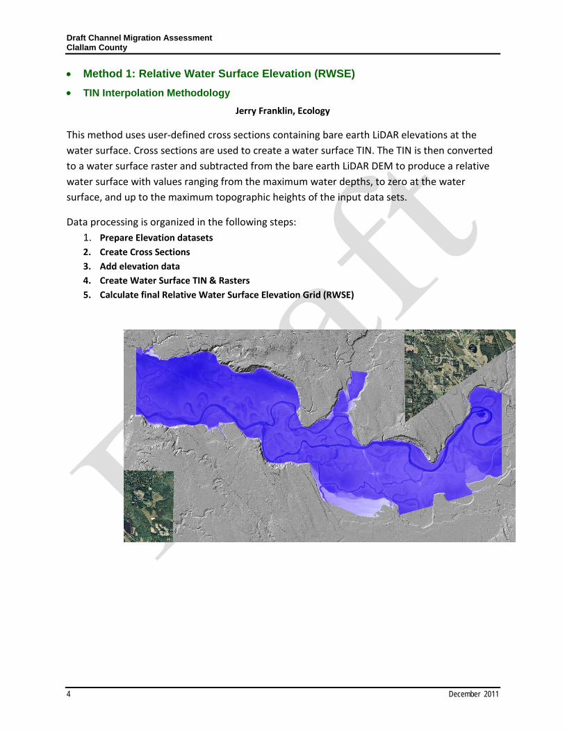
• Method 1: Relative Water Surface Elevation (RWSE) • TIN Interpolation Methodology
Jerry Franklin, Ecology
This method uses user-defined cross sections containing bare earth LiDAR elevations at the water surface. Cross sections are used to create a water surface TIN. The TIN is then converted to a water surface raster and subtracted from the bare earth LiDAR DEM to produce a relative water surface with values ranging from the maximum water depths, to zero at the water surface, and up to the maximum topographic heights of the input data sets.
Data processing is organized in the following steps: 1. Prepare Elevation datasets 2. Create Cross Sections 3. Add elevation data 4. Create Water Surface TIN & Rasters 5. Calculate final Relative Water Surface Elevation Grid (RWSE)
Draft Channel Migration Assessment Clallam County
5 December 2011
Elevation dataset preparation
• Mosaic ‘Bare Earth’ LiDAR tiles if necessary to create one continuous surface for analysis ArcToolbox [data management tool|raster|mosaic to new raster] [set cell size to 6’ (equal to LiDAR)]
• Create shaded relief Spatial Analyst [surface analysis|hillshade] [set cell size to 6’ (equal to LiDAR)]
[name file and specify output location] Use 3D Analyst to determine cross section extent Cross Sections
• Create cross sections of the valley floor perpendicular to the mainstem Use [New line graphic tool]
Draft Channel Migration Assessment Clallam County
6 December 2011
• Use Xtools Pro to Convert Graphics to Shapes Select all graphic lines
[xtools pro|feature conversions|convert graphics to shapes] Name shapefile “xsections”
Calculate elevation values
• Add elevation to attribute table Open cross section attribute table
[OPTIONS| addfield| Name: ‘elev’|Type:Double]
• Edit attribute table to add elevations from LiDAR shade relief [Editor|start editing] Label the cross section shapefile to see ID’s Open cross section attribute table and move aside to view the LiDAR shaded relief
• Extract Bare Earth DEM’ elevation values Using the shaded relief as a guide, use the Identity Tool to Identify from the ‘Bare Earth DEM‘ elevation pixel values where the cross sections intersect with the mainstem. [It is important to extract water surface elevations from the Bare Earth DEM] Manually enter pixel values into attribute table by selecting the ‘elev’ cell of the corresponding polyline and typing in the pixel value
• When done entering all elevation values [ Editor|stop editing|save edits]
Draft Channel Migration Assessment Clallam County
7 December 2011
• Convert Features to 3D for use in creating Relative Water Surface Raster TIN 3D Analyst: [Convert Features to 3D] Input features = xsect.shp Source of heights Input feature attribute: ‘elev’ Output 3D xsection shapefile
Create Rasters
• Create a Raster Tin from 3D cross sections [3D Analyst: Create/Modify Tin| Create TIN from features] input layer= 3D xsection shapefile
height source = ‘Elev’ triangulate as = ‘hardline’ output TIN
The resulting TIN should appear similar to the image above
Draft Channel Migration Assessment Clallam County
8 December 2011
• Create Raster Grid from the 3D TIN to subtract the RWSE grid from the Bare Earth elevation grid. [3D Analyst| convert Tin to Raster] Input TIN = wse_tin Attribute = Elevation Z factor = 1.000 Cell size = 6 (the cell size of Bare Earth grid) Output RWSE Raster
Open the resulting grid properties and change the symbology to stretched and a color ramp of blue. The grid should appear similar to the image above. Create final Relative Water Surface Elevation Grid (RWSE)
Each cell of the RWSE grid should contain values of zero at the water surface taken from the Bare Earth grid and range from the greatest elevation difference above and below the extracted water surface elevation (e.g. zero at the water surface to six feet of bathymetry below the water and hundreds of feet of topography above the water.)
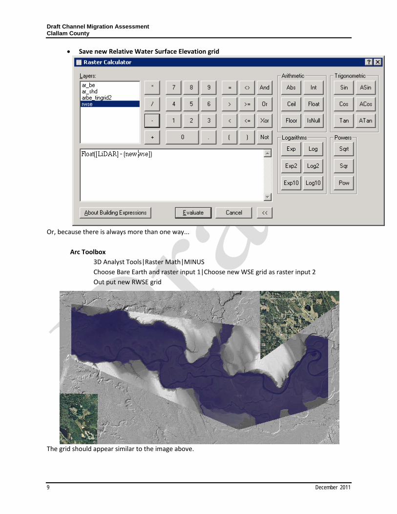
• Spatial Analyst – Raster Calculator (Subtract Raster_WSE from LiDAR) Expand the calculator [Choose the ‘Float’ Arithmetic function] [Choose the Bare Earth grid first, subtraction, then choose the new wse grid] [Evaluate] The calculation should look as follows: Float([LiDAR]-[new wse])
Draft Channel Migration Assessment Clallam County
9 December 2011
• Save new Relative Water Surface Elevation grid Right click on the calculation grid in the Table of Contents and select “Make Permanent”
Or, because there is always more than one way...
Arc Toolbox 3D Analyst Tools|Raster Math|MINUS
Choose Bare Earth and raster input 1|Choose new WSE grid as raster input 2 Out put new RWSE grid
The grid should appear similar to the image above.
Draft Channel Migration Assessment Clallam County
10 December 2011
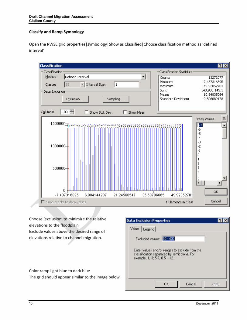
Classify and Ramp Symbology Open the RWSE grid properties|symbology|Show as Classified|Choose classification method as ‘defined interval’ Choose ‘exclusion’ to minimize the relative elevations to the floodplain Exclude values above the desired range of elevations relative to channel migration.
Color ramp light blue to dark blue The grid should appear similar to the image below.
Draft Channel Migration Assessment Clallam County
11 December 2011
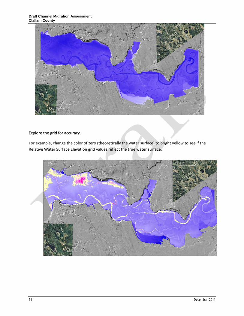
Explore the grid for accuracy.
For example, change the color of zero (theoretically the water surface) to bright yellow to see if the Relative Water Surface Elevation grid values reflect the true water surface.
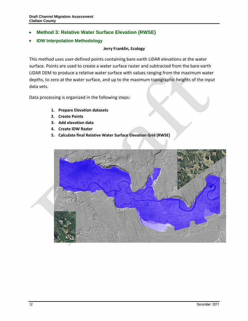
This method uses user-defined points containing bare earth LiDAR elevations at the water surface. Points are used to create a water surface raster and subtracted from the bare earth LiDAR DEM to produce a relative water surface with values ranging from the maximum water depths, to zero at the water surface, and up to the maximum topographic heights of the input data sets.
Data processing is organized in the following steps:
1. Prepare Elevation datasets 2. Create Points 3. Add elevation data 4. Create IDW Raster 5. Calculate final Relative Water Surface Elevation Grid (RWSE)
Draft Channel Migration Assessment Clallam County
13 December 2011
Elevation dataset preparation
• Mosaic ‘Bare Earth’ LiDAR tiles if necessary to create one continuous surface for analysis ArcToolbox [data management tool|raster|mosaic to new raster] [set cell size to 6’ (equal to LiDAR)]
• Create shaded relief Spatial Analyst [surface analysis|hillshade] [set cell size to 6’ (equal to LiDAR)]
[name file and specify output location] Use 3D Analyst to determine cross section extent Elevation Points
• Create points along the mainstem watersurface Use [New point graphic tool]
Draft Channel Migration Assessment Clallam County
14 December 2011
• Use Xtools Pro to Convert Graphics to Shapes Select all points
[xtools pro|feature conversions|convert graphics to shapes] Name shapefile “wse_pnts”
Calculate elevation values
• Add elevation to attribute table ArcToolbox [Spatial Analyst Tools|Extraction|Extract Values to points]
Input Point Feature = wse_pnts Input Raster = Bare Earth LiDAR
Output shapefile = wse_pnt_el The resulting table should contain elevation values at the intersection of the point file and raster dataset.
This function will add an attribute to the output point file “rastervalu’ Add a new field called ‘elev’ and calc ‘elev’ = ‘rastervalu’
• Add elevation attribute to table Open point attribute table
[OPTIONS| addfield| Name: ‘elev’|Type:Double]
[right click on the title ‘rastervalu’|Options :delete field]
Create Raster using IDW Interpolation function
ArcToolbox [Spatial Analyst Tool|Interpolation|IDW] input point featurer= 3D pointfile Z value = ‘Elev’ Output Cell size = 6 Choose Environments at the bottom of the box Choose General Settings Extent = same as bare earth LiDAR extent
Draft Channel Migration Assessment Clallam County
15 December 2011
The grid should appear similar to the image above. Export the resulting ‘calculation’ file as a grid; cell size = 6
Open the resulting grid properties and change the symbology to stretched and a color ramp of blue. The grid should appear similar to the image above. Create final Relative Water Surface Elevation Grid (RWSE)
Each cell of the RWSE grid should contain values of zero at the water surface taken from the Bare Earth grid and range from the greatest elevation difference above and below the extracted water surface elevation (e.g. zero at the water surface to six feet of bathymetry below the water and hundreds of feet of topography above the water.)
• Spatial Analyst – Raster Calculator (Subtract Raster_WSE from LiDAR) Expand the calculator [Choose the ‘Float’ Arithmetic function]
Draft Channel Migration Assessment Clallam County
16 December 2011
[Choose the Bare Earth grid first, subtraction, then choose the new wse grid] [Evaluate] The calculation should look as follows: Float([LiDAR]-[new wse])
• Save new Relative Water Surface Elevation grid Right click on the calculation grid in the Table of Contents and select “Make Permanent”
Or, because there is always more than one way...
Arc Toolbox 3D Analyst Tools|Raster Math|MINUS
Choose Bare Earth and raster input 1|Choose new WSE grid as raster input 2 Out put new RWSE grid
The grid should appear similar to the image above.
Draft Channel Migration Assessment Clallam County
17 December 2011
Classify and Ramp Symbology Open the RWSE grid properties|symbology|Show as Classified|Choose classification method as ‘defined interval’ Choose ‘exclusion’ to minimize the relative elevations to the floodplain Exclude values above the desired range of elevations relative to channel migration.
Color ramp light blue to dark blue The grid should appear similar to the image below.
Draft Channel Migration Assessment Clallam County
18 December 2011
Explore the grid for accuracy.
For example, change the color of zero (theoretically the water surface) to bright yellow to see if the Relative Water Surface Elevation grid values reflect the true water surface.