190
APPENDIX F Attachments from Comment Letter U

APPENDIX F Attachments from Comment Letter U


APPENDIX F-1 EH City Creek Scour Analysis Final Report


Engineering & Hydrosystems Inc.
Engineering & Hydrosystems Phone 303-683-5191
8122 SouthPark Lane Fax 303-683-0940
Littleton, CO 80120
City Creek
Scour Analysis for Inland Feeder Pipeline Crossing
Prepared for:
Black & Veatch 6300 South Syracuse Way, #300 Centennial, CO 80111

I
Table of Contents
INTRODUCTION......................................................................................................................................................1
OBJECTIVE..............................................................................................................................................................3
PROJECT APPROACH...........................................................................................................................................3
Problem Definition .................................................................................................................................................3
Reach Degradation ...............................................................................................................................................3
Local Scour............................................................................................................................................................5
Combined Effect....................................................................................................................................................6
Approach................................................................................................................................................................6
AVAILABLE DATA ...................................................................................................................................................7
METHODOLOGY.....................................................................................................................................................7
Geomorphic Characterization...............................................................................................................................7
Hydrology Analysis................................................................................................................................................7
Hydraulic Modeling................................................................................................................................................8
Bed Material Characterization ..............................................................................................................................8
Scour Analyses....................................................................................................................................................10
RESULTS ...............................................................................................................................................................17
Geomorphic Characterization.............................................................................................................................17
Field Reconnaissance.........................................................................................................................................17
Existing Topography ...........................................................................................................................................23
Historical Morphologic Analysis..........................................................................................................................25
Hydrology.............................................................................................................................................................26
Hydraulics ............................................................................................................................................................27
Material Characterization ....................................................................................................................................30

II
Bed Material Gradation .......................................................................................................................................30
Erosion Resistance .............................................................................................................................................30
Scour Analysis.....................................................................................................................................................31
Reach Degradation .............................................................................................................................................31
Local Scour..........................................................................................................................................................36
SUMMARY .............................................................................................................................................................38
DESIGN ALTERNATIVES.....................................................................................................................................38
Channel Widening without Boundary Hardening ..............................................................................................41
Riprap Chute........................................................................................................................................................41
Single Vertical Drop Structure ............................................................................................................................42
Multiple Grade Control Structures ......................................................................................................................43
REFERENCES.......................................................................................................................................................44
APPENDIX A – HYDROLOGY CALCULATIONS ..............................................................................................A-1
APPENDIX B – HEC-RAS MODEL.....................................................................................................................B-1
APPENDIX C – ERODIBILITY INDEX METHOD...............................................................................................C-1
APPENDIX D – ARMOR LAYER ........................................................................................................................D-1
APPENDIX E – STABLE SLOPE........................................................................................................................E-1
APPENDIX F – BEND SCOUR ........................................................................................................................... F-1
APPENDIX G – HEADCUT HYDRAULICS ........................................................................................................G-1
APPENDIX H - BLACK & VEATCH RIPRAP GRADATION CALCULATIONS.................................................H-1

III
LIST OF FIGURES
Figure 1. Site Location Map (Obtained From Google Earth) .................................................................................2
Figure 2. Schematic of Lane's Stream Balance (Taken from Rosgen 1996 after Lane 1955).............................4
Figure 3. Erosion Threshold for Earth Materials with Erodibility Index K > 0.1 (Annandale 1995; 2006) ............9
Figure 4. Erosion Threshold for Earth Materials With Erodibility Index K < 0.1 (Annandale 1996; 2006) ..........10
Figure 5. Pipeline Crossing Cross Section...........................................................................................................13
Figure 6. Flow Around a Bend, Showing Spiraling Transverse Flow and Longitudinal Flow (Annandale 2006)14
Figure 7. Headcut Hydraulics (Annandale 2006) ..................................................................................................15
Figure 8. City Creek Exiting San Bernardino National Forest..............................................................................18
Figure 9. City Creek Entering Santa Ana River....................................................................................................19
Figure 10. Photo of the Pipeline Crossing (Upstream is on the Right)................................................................19
Figure 11. City Creek at Highland Ave Looking Downstream .............................................................................20
Figure 12. Channelization of City Creek (Base Line St and Boulder Ave in Background), Looking Downstream20
Figure 13. Schematic of Historic, Current, and Possible Future Geomorphic Conditions of City Creek............21
Figure 14. City Creek Downstream of Baseline Street ........................................................................................22
Figure 15. Headwall of Mining Pit In Floodplain Downstream of Baseline Street...............................................22
Figure 16. City Creek Longitudinal Profile Indicating Head Cut Locations..........................................................24
Figure 17. Photograph of City Creek in 2003 .......................................................................................................25
Figure. 18 Photograph of City Creek in 2005 .......................................................................................................25
Figure 19. Location of USGS Stream Flow Gage 11055800 ...............................................................................27
Figure 20. Pipeline Cross-sections Used for the HEC-RAS Models ...................................................................28
Figure 21. Average Flow Velocities at Pipeline Crossing (Calculated with HEC-RAS)......................................28
Figure 22. Shear Stress at Channel Bottom at Pipeline Crossing (Calculated with HEC-RAS) ........................29
Figure 23. Stream Power at Channel Bottom at pipeline crossing (Calculated with HEC-RAS) ........................29
Figure 24. Bed Material Gradation (Chang 1995).................................................................................................30

IV
Figure 25. Existing Grain Size Distribution and Calculated Armor Layer D50 for All Four Geometries Evaluated ................................................................................................................................................................32
Figure 26. Predicted Armor Layer Gradation Using Gessler (1970) Compared to Existing Bed Material Gradation at Pipeline Crossing. .............................................................................................................................33
Figure 27. Estimated Scour Depths Associated With Armor Layer Formation...................................................34
Figure 28. Location and Dimensions of Bend Analyzed.......................................................................................37
Figure 29. Three-Dimensional Image of Calculated Bend Scour at the Pipeline Crossing................................37
Figure 30. Conceptual Configuration of Riprap Lined Rock Chute. Exact Dimensions to be Determined During Preliminary and Final Design. ................................................................................................................................42
Figure 31. Conceptual Sketch of Single Drop Structure. .....................................................................................42
Figure 32. Multiple Rock Chutes...........................................................................................................................43
LIST OF TABLES
Table 1. Available Data ............................................................................................................................................7
Table 2. City Creek Flood Peak Discharges .........................................................................................................26
Table 3. Threshold Stream Power at Pipeline Crossing ......................................................................................30
Table 4. Armor Layer Particle Diameter and Associated Depth of Degradation Results at the Pipeline Crossing..................................................................................................................................................................32
Table 5. Armor Layer Particle Diameter and Associated Depth of Degradation Results at Existing Headcuts33
Table 6. Base Level Information and Estimated Time for Stable Conditions to Establish if Median Bed Material Particle Size Dominates in the Determination of Quasi-Equilibrium Conditions ..................................................35
Table 7. Estimated Stable Slope, Depth of Degradation, and Rate of Scour at Pipeline Crossing Assuming Median Bed Material Diameter Control .................................................................................................................35
Table 8. Comparison Between Stream Power in Bend and Erosion Threshold.................................................36
Table 9. Backroller Stream Power Associated with Active Headcuts .................................................................38
Table 10. Optional Mitigation Measures ...............................................................................................................40
Table 11. Comparison of Erosive Capacity of Water for Design Flood Conditions and the Threshold Stream Power of an Armor Layer that is Expected to Form Under Such Conditions.......................................................41

DRAFT: 2/22/06 1
INTRODUCTION
The Inland-Feeder Pipeline runs beneath City Creek in the reach between Highland Avenue and Boulder Avenue in Southwest San Bernardino County, California (Figure 1). The 12-foot diameter pressurized pipeline was originally buried 20 feet below the City Creek thalweg (Chang 1995). The creek experienced relatively high discharges during the winter of 2004/2005, which led to flooding concerns. As a consequence, the conveyance capacity of the creek was increased by excavating an earthen trapezoidal channel in the stream reach of interest, with a length of about 1.5 miles. The excavation changed the channel morphology from a braided stream to a single-thread stream with a consequent change in hydraulic characteristics. The erosive capacity in the single-thread stream is greater than that of a braided stream, resulting in increased scour at the crossing. An initial rough estimate indicated that the amount of cover above the pipeline has decreased by 8 to 10 feet. At this time, it is not clear if this is due to construction activities or the new channelized conditions. Metropolitan Water District (MWD) requested Engineering & Hydrosystems Inc. (E&H) to evaluate the risk posed to the pipeline by the altered hydraulic and sediment transport regime and to propose mitigation measures, if necessary.

DRAFT: 2/22/06 2
Figure 1. Site Location Map (Obtained From Google Earth)

DRAFT: 2/22/06 3
OBJECTIVE
The objective of this investigation is to determine if the existing soil cover above the Inland Feeder Pipeline is adequate to protect it against future scour that may occur within City Creek. If the cover is inadequate mitigation measures are be proposed and evaluated for fatal flaws.
PROJECT APPROACH
Problem Definition
Changing the fluvial geomorphologic characteristics of City Creek from a braided to a single-thread stream in the vicinity of the Inland Feeder Pipeline crossing concentrates the erosive capacity of the water on the bed of the excavated channel. This concentration in the water results in increased erosion, characterized as reach degradation and local scour. Reach degradation is the result of erosion along a stream reach, i.e. a general decrease in average reach elevations. Local scour is a response to hydraulic action at local stream irregularities. Such stream irregularities increase the local turbulence intensity in the flowing water, resulting in local lowering of the stream bed. By quantifying the reach degradation and local scour it is possible to assess the risk of stream degradation to the Inland Feeder Pipeline.
Reach Degradation
Reach degradation is the result of erosion manifested over a long river reach (say e.g. between Highlands Avenue and Baseline Avenue, or an even longer distance). When general erosion occurs over a stream reach the average bed elevations along the river reach decrease. Degradation will continue until the variables determining stream channel characteristics are in balance. This is known as a quasi-equilibrium condition, due to the fact that flow variability will always result in varying channel geometry, within certain limits.
The principal parameters determining stable reach conditions are water discharge, sediment properties and channel geometry. A simplified explanation of the relationship between stable reach conditions and the variables determining quasi-equilibrium is given by Lane (Figure 2). This simplification of fluvial geomorphic response to changes in hydrologic, geometric and sediment characteristics in river systems is useful for conceptually understanding and explaining river behavior.
Lane’s balance indicates that a river is in quasi-equilibrium (i.e. in balance) for a particular combination of water discharge, sediment characteristics, and channel geometry. The sediment characteristics are represented by sediment load (shown on the left hand scale bucket) and by sediment diameter (represented by the scale on the left arm of the balance). The bucket containing the sediment load can be moved to the left or right along the left arm of the scale, depending on the representative diameter of the sediment. Coarsening of the sediment requires moving the scale pan containing the sediment to the left. If the sediment diameter decreases in size, the scale pan is moved to the right. A change in sediment load, i.e. either an increase or decrease in load, is represented by changing the amount of sediment on the scale pan.
Similarly, the amount of water discharging in the river is represented by the jug containing water on the right hand side of the balance. The geometric characteristics of a river or creek are represented by longitudinal slope. If the river or creek slope increases, the pan containing the

DRAFT: 2/22/06 4
water is moved towards the right. If the slope decreases, the pan is moved towards the left. Additionally, if the discharge in the river or creek increases, the amount of water in the jug on the right hand scale pan is increased.
The anticipated fluvial geomorphologic response of a river or creek is determined by making observations on the movement of the indicator in the middle of the scale. If the scale tips towards the right, the indicator moves towards the left, indicating degradation. Alternatively, if the scale tips towards the left, the pointer moves towards the right indicating aggradation.
Figure 2. Schematic of Lane's Stream Balance (Taken from Rosgen 1996 after Lane 1955)
For example, to interpret the anticipated response of City Creek to the channelization project one proceeds as follows. By changing the channel characteristics from a braided channel to a single channel, the amount of discharge is effectively increased. This is deduced from the fact that the amount of discharge per channel in a braided system is less than the combined discharge in a single-thread channel. Additionally, the average channel slope has been increased because of the reduction in sinuosity. A braided channel is much more sinuous than the straight, channelized reach. Therefore, by increasing the amount of water in the jug shown in the Lane diagram (representing the increased concentration of flow in the channel) and by moving the scale pan containing the jug to the right (indicating an increase in slope), one expects the scale pointer to move towards the left; indicating degradation.
An important part of the reach analysis is to quantify the relationship between sediment characteristics, water discharge and channel slope. The objective of such an analysis is to quantify the long-term stable reach slope. Such an analysis assumes that the sediment and water discharge characteristics are known.
The water discharge characteristic is represented by the magnitude of what is known as the channel-forming discharge, which is normally defined as approximately equal to the 2-year

DRAFT: 2/22/06 5
recurrence interval discharge (Annable1994 and Andrews1980). This is a discharge that occurs on a regular basis, regular enough to exert a dominant impact on the long term characteristics of a stream reach.
When considering the impact of sediment characteristics on the long term stable stream slope it is necessary to account for the characteristics of the bed material gradation. Stream bed material gradations can consist of fine material only, coarse material only, or a combination of fine and coarse material. Coarse material is defined, somewhat arbitrarily, as sediment particles that cannot be moved by the water flowing in the stream during channel-forming discharge.
From a stable slope analysis point of view, the scenarios where the bed material consists of almost uniformly distributed fine or coarse particles, the long term stable slope can be related to the median diameter of the bed material. This is done by making use of established techniques relating discharge, sediment particle diameter and channel slope. These methods are identified in the report section dealing with methodology.
Should the bed material gradation consist of both fine and coarse material, an additional analysis is required. In such cases it is possible that the coarse material can form an armor layer consisting of the coarsest sediment particles in the bed material mix. An armor layer develops when the fine sediment particles that can be removed by the flowing water have been removed and are no longer present in the top layer of the bed material. In such a case only the coarse material remains in the top stream bed material layer. The latter forms a continuous layer along the bed surface and protects the underlying fine material from scour. Experience has shown that the formation of armor layers is possible if the amount of coarse material in the sediment gradation equals 10% or more (Pemberton and Lara 1984).
Once it has been established that it is possible for an armor layer to form, it is necessary to determine the amount of scour that will occur before the layer is in place. This scour occurs due to the removal of fine particles from the upper layer of the bed material. If it is desired to know the stable slope of the stream once an armor layer has established, the amount of scour prior to armor layer formation at various locations along the stream reach is determined. Connecting these elevations it is possible to develop an estimate of the stable long section of the stream. Methods for determining the potential for armor layer formation and the amount of scour that will occur prior to armor layer formation are presented in the section dealing with methodology.
Local Scour
Local scour occurs due to increased flow turbulence developing in the immediate vicinity of an irregularity in stream geometry. Such irregularities include bridge piers, flow contraction due to the presence of bridge abutments, and irregularities in a stream bed profile, such as headcuts. A headcut is a sudden drop in a river bed. When a water jet discharges over a drop it can lead to the formation of a backroller between the upstream, vertical face of the headcut and the point of jet impact. If the erosive capacity of the water in the backroller is greater than the ability of the earth material in the headcut face to resist erosion, this material will erode and the headcut will move upstream. This action is known as headcut migration. The magnitude of the erosive capacity of water in the immediate vicinity of local irregularities is usually significantly greater than the erosive capacity of water merely flowing over a stream bed with a regular, continuous slope. Therefore, the rate of scour at irregularities is usually greater than that associated with reach degradation.

DRAFT: 2/22/06 6
Combined Effect
The total scour at the pipeline crossing is the sum of the reach degradation and local scour. When combining the quantitative results of the analyses, appropriate interpretation of results is required. The long term elevations of the stream thalweg is represented by the maximum elevations of either the stable slope determined using the median particle diameter of the sediment gradation or that associated with the degradation of the stream bed associated with the formation of bed armoring.
The process of combining the local scour estimates with the long term stable thalweg depends on the kind of local scour. If the local scour is the result of bridge pier scour or contraction scour between bridge abutments, it is normally subtracted from the long term stable bed profile. This is justified if an armor layer that formed on the bed is unable to resist the increase in erosive capacity of the water at these irregularities.
If the local scour is due to the presence of headcuts these are normally not subtracted from the stable bed elevation. The reason for this is that headcuts are interpreted as geomorphic processes accelerating the river processes leading to long term stability. These processes are perceived to occur during the interim phases, prior to establishment of the long term stable reach slope.
Approach
The approach followed in this investigation entails combining fluvial geomorphologic and fluvial hydraulic expertise and experience to assess scour potential at the Inland Feeder Pipeline crossing at City Creek. As standard practice, E&H takes a watershed approach to geomorphic investigations. In order to understand the erosion/deposition processes at a single cross section, which in this case is the pipeline crossing, it is imperative to understand the processes occurring within the system, i.e. the watershed.
By following this approach the investigation included visiting the site, conducting a fly-over with a helicopter provided by MWD, and conducting detailed scour analyses using fluvial geomorphologic and fluvial hydraulic principles. This assessment entailed conducting a fluvial geomorphologic characterization of the watershed and the stream reach up to the confluence with the Santa Ana River, followed by hydrologic and hydraulic analyses, stream bed material characterization, and, finally, a scour analysis. The latter consisted of quantifying reach degradation and local scour as conceptually outlined in the previous section. Once the extent of long term erosion has been quantified, the risk of pipeline exposure was determined and optional protection techniques identified for safeguarding the pipeline crossing against the effects of scour.

DRAFT: 2/22/06 7
AVAILABLE DATA
In order to conduct our analyses, the hydrology, geometry, bed material characteristics, and historical condition of the reach are required. Table 1 lists the data collected and used for our analyses.
Table 1. Available Data
Source Data MWD Photographs of City Creek (pre and post channelization) MWD Chang, Howard H. 1995. Inland Feeder Pipeline, San
Bernardino Segment (Contract 3): Fluvial Study of City Creek for Pipeline Placement. Prepared for Dames and Moore
MWD Bridge surveys of Highland Avenue, Baseline Street, and Boulder Avenue
MWD AutoCAD topographical map of site created from surveyed data
USGS Annual peak stream flow data from USGS gage 11055800 for the period of record (1920-2004)
METHODOLOGY
Geomorphic Characterization
Geomorphic characterization of the watershed is critical for understanding the potential mechanisms for scour. A geomorphic analysis involves studying the current field conditions, site topography and historical site and watershed conditions. Current field conditions including vegetation, presence/absence of headcuts, condition of tributaries, bank shape and steepness, viewed in terms of the fluvial geomorphologic balance represented by Figure 2, allow an interpretation of the current channel stability. Topographic maps of the site enhance the field information by allowing detailed calculations of the stream morphometry. Historical analysis of stream channel plan form using current and historical aerial photographs and investigations of the changes in the longitudinal stream profile using current and historic topographic maps and surveys add to the interpretation of the condition of the creek or river, and potential future trends.
Hydrology Analysis
The scour analysis required peak discharge magnitudes associated with the 2- and 100-year recurrence intervals. Chang (1995) provides hydrologic data, i.e. peak discharges for the 10-year, 50-year, 100-year 3-hour, 100-year 24-hour, and the Standard Project Flood (SPF). For this investigation, the channel-forming discharge was also required.
Channel forming discharge is the discharge that is assumed to play the dominant role in determining the long-term morphology of a river or stream, which is of principal interest in this investigation. The channel-forming discharge for City Creek was assumed to be represented
DRAFT: 2/22/06 8
by the 2-year recurrence interval flow. The selection of a 2-year recurrence interval flow implies that the long-tem morphology of rivers is determined by flows that occur on a regular basis. This, of course, does not mean that major floods, such as a 50- or 100- year flood, will not affect morphometry. On the contrary, such floods affect short term response of river and creek morphometry and should be accounted for in infrastructure design.
The 2-yr discharge for City Creek was calculated using a log Pearson type III analysis. The log Pearson type III is a type of probability distribution used in the United States for relating flood-peak magnitude and probability of occurrence (Haan et al. 1994). Yearly peak discharge data was obtained from USGS gage 11055800, located on City Creek approximately one mile upstream of the Pipeline crossing. This gage provided 85 years of annual peak discharge data. The calculations are contained in Appendix A.
Hydraulic Modeling
It is necessary to quantify the hydraulic parameters associated with the 2-yr and 100-yr flows at the crossing and along the creek to calculate the potential scour depth. The hydraulic characteristics of the 2-yr flood were used to estimate long term stable creek conditions; while those of the 100-year flow are used to assess short term, i.e. event-based, impacts.
The HEC-RAS software was used to quantify the hydraulic parameters of the creek. HEC-RAS v. 3.1.3 (USACE 2005) is a software package that can perform one-dimensional steady flow and unsteady flow hydraulic calculations for networks of natural and constructed channels. Developed by the Hydrologic Engineering Center at the U.S. Army Corps of Engineers, the system comprises a graphical user interface, separate hydraulic analysis components, data storage and management capabilities, and graphics and reporting facilities. Data requirements include channel geometry, flow data and hydraulic boundary conditions. HEC-RAS model input and output are included in Appendix B.
Bed Material Characterization
Bed material characterization entails quantifying the physical properties and erosion resistance of the stream bed material. In the case of City Creek the bed material consists of non-cohesive sediment and physical characterization is accomplished by conducting gradation analyses on the earth material. Determination of the erosion resistance of the bed material can be accomplished by making use of acknowledged methods, such as the Shields (1936) diagram and the Erodibility Index Method (EIM) (Annandale 1995). The principal method for quantifying erosion resistance used during the course of this project is the EIM. This method has been used for a number of years and has been shown to correlate favorably with field experience (Annandale 2006). However, other methods, including the Shields diagram, are used to estimate reach degradation.
The EIM defines a threshold between erosion and non-erosion by relating the erosive capacity of water, expressed in terms of stream power, and the relative ability of earth material to resist erosion, expressed in terms of the erodibility index (Appendix C). The index is the scalar product of the values of its constituent parameters and takes the form:
K = Ms * Kb * Kd * Js (0.1) Ms = mass strength number Kb = particle/block size number = 1000 * (d (in meters))3 for non-cohesive particulate matter Kd = discontinuity or inter-particle bond shear strength number = tangent of the angle of internal friction in the case of non-cohesive particulate matter

DRAFT: 2/22/06 9
Js = relative ground structure number d = characteristic particle size; = median particle size in the case of no armoring; = armor material size in the presence of armoring.
The numbers identified above are quantified by making use of tables in Annandale (1995, 2006). The Erodibility Index K for a particular earth material is used to determine the threshold stream power per unit area. If the stream power of the water is greater than the threshold stream power, the earth material will erode. If it is lower, the earth material will not erode. The erosion thresholds for earth materials with K > 0.1 and K < 0.1, respectively, are shown on Figure 3 and Figure 4.
The stream power exerted by the water can be obtained from the HEC-RAS model for open channel flow conditions. It is quantified by analytical means for other flow conditions, such as those present at bridge piers, headcuts and hydraulic jumps (Annandale 2006).
Figure 3. Erosion Threshold for Earth Materials with Erodibility Index K > 0.1 (Annandale 1995; 2006)
0.1
1
10
100
1000
10000
1.00E-02 1.00E-01 1.00E+00 1.00E+01 1.00E+02 1.00E+03 1.00E+04
Erodibility Index
Stre
am P
ower
KW
/m2
Erosion
No Erosion

DRAFT: 2/22/06 10
Figure 4. Erosion Threshold for Earth Materials With Erodibility Index K < 0.1 (Annandale 1996; 2006)
Scour Analyses
Reach Degradation
Pemberton and Lara (1984) outline an analytical approach for implementing the concept of the Lane balance (Figure 2) in practice, i.e. estimating reach degradation and quantifying the long term stable slope for quasi-equilibrium conditions. It is important to note that analytical techniques contained in this publication do not address streambed and/or valley controls such as rock outcrops, vegetation, or manmade changes. “A control in the channel may in some cases prevent any appreciable degradation from occurring above it. Conversely, a change or removal of an existing control may initiate the degradation process (Pemberton and Lara 1984).”
Reach Degradation Associated with Armor Layer Formation The formation of an armor layer is associated with bed scour, which results due to the removal of fine bed material particles subject to erosion. Once the fine particles have been removed and the armor layer has established, scour ceases. Reach degradation associated with the formation of armor layers is therefore equal to the amount of overall degradation occurring prior to armor layer formation. Pemberton and Lara (1984) recommend using the following five methods for estimating the characteristic armor layer particle size (see Appendix D for detail):
1. Meyer-Peter, Muller sediment transport equation,
2. Competent bottom velocity method;
3. Lane’s tractive force theory;
4. Shields diagram; and
0.000001
0.00001
0.0001
0.001
0.01
0.1
1
1E-11 1E-10 1E-09 1E-08 0.0000001 0.000001 0.00001 0.0001 0.001 0.01 0.1 1
Erodibility Index
Stre
am P
ower
(kW
/m2)
Erosion
No Erosion

DRAFT: 2/22/06 11
5. Yang incipient motion
Gessler (1970) established a method that was found to be very useful for estimating armor layer characteristics. This method is more detailed and has been found to provide satisfactory results when compared to field observations (Oehy 1999). A unique feature of the Gessler method is that it results in a sediment gradation curve of the armor layer. This method has also been used to estimate the armor layer characteristics.
Once the physical characteristics of the armor layer are known, the amount of scour is calculated by making use of an equation recommended by Pemberton and Lara (1984), i.e.
d a1y y 1p
= − ∆ (0.2)
where dy = amount of scour, measured in the vertical direction; ay = thickness of the armor
layer; p∆ = percentage of material in the original bed material gradation that is equal to or exceeds the armor layer particle size.
Example calculations and results when implementing these six methods for determining armor layer size and using equation (0.2) to estimate scour associated with armor layer formation are included in Appendix D.
Reach Degradation in the Absence of Armor Layer Formation
Reach degradation associated with flow conditions in the absence of armor layer formation is a function of the difference between the stream slope prior to establishment of stable flow conditions and that after establishment of stable flow conditions, as previously outlined. Streams subject to degradation will decrease their longitudinal slope until a new level of equilibrium is reached. As degradation occurs the longitudinal slope of the river gradually decreases, and, with it, the erosive capacity of the water. Once the erosive capacity of the water is equal to the erosion threshold of the bed material a stable slope has been established.
The methods implemented by Pemberton and Lara (1984) for calculating stable slope include (see Appendix E for detail on implementing these methods):
1. Schoklitsch bedload equation;
2. Meyer-Peter Muller sediment transport equation;
3. Shields diagram; and
4. Lane’s relationship for critical tractive force assuming clear water-flow in canals.
The results obtained by implementing the four methods listed above are interpreted and a long term stable slope for the stream assigned.
Local Scour
Mechanisms of local degradation include contraction scour, pier scour, abutment scour, bed form scour (dune formation and propagation), headcut migration, bend scour, and low-flow channel incisement. During the field investigation it was determined that contraction scour; pier

DRAFT: 2/22/06 12
scour, abutment scour, bed form scour and low-flow channel incisement would not be the large-scale factors influencing bed stability at the Pipeline. The only two significant local scour features identified are bend scour and headcut migration.
Bridge pier and contraction scour were not considered due to the fact that these scour types do not currently affect scour at the pipeline. The Pipeline crossing is not within the limits of any pier or abutment scour associated with the Highland Avenue or Baseline Street bridges.
Additionally, the Highland Avenue Bridge crossing contains a concrete apron overlying the earth material. The crossing at Baseline Street is a concrete box culvert. The concrete linings will protect this infrastructure against the effects of scour as long as they remain in place. It is therefore important to prevent scour occurring just downstream of these concrete aprons from destroying the aprons themselves. Significant scour just downstream of the Highland Avenue Bridge is already present. Gravel mining downstream of the Baseline Street crossing (see discussion further on) may also have an adverse impact on the long term stability of this culvert. Should scour just downstream of the creek crossings destroy the protective layer provided by the concrete linings, the additional scour may have an adverse effect on scour at the Inland Feeder Pipeline crossing.
The particle sizes present in the bed are not prone to dune formation or dune migration. We therefore expect that dune formation will play an insignificant role.
Low-flow channel incisement can potentially pose problems if not taken into account in the mitigation design. Figure 5 indicates incision may have already occurred. However, although low-flow channel incisement currently appears to play a role, the channel is expected to assume a braided condition in the long term (decades from now), with relatively small channel depths. (This assessment is discussed below in GEOMORPHIC CHARACTERIZATION section.) Therefore, low-flow incisement would be a relatively insignificant amount of scour relative to the overall long-term degradation. When developing mitigation designs it should be prepared in a manner that will encourage formation of a braided channel configuration. Low-flow channel incisement potential has therefore not been investigated as it will be accounted for in the mitigation design.
The principal local scour features considered in this investigation are bend scour and headcut migration.

DRAFT: 2/22/06 13
1425
1430
1435
1440
1445
1450
1455
1460
0 50 100 150 200 250 300
Station (ft)
Elev
atio
n (ft
)
Figure 5. Pipeline Crossing Cross Section
Bend Scour The potential for and the magnitude of bend scour are determined by first quantifying the magnitude of the stream power of the water flowing around the bend, and comparing it with the erosion threshold of the material in the stream bed. Once it has been established that the bed material can potentially scour, i.e. the erosion threshold is exceeded when water flows around the bend, then the magnitude of the scour is determined by making use of a three-dimensional analytical model.
The magnitude of the stream power flowing around a bend can be calculated by making use of a method described by Annandale (2006). The total stream power around a bend can be quantified as,
total channel bendP P P= + (0.3)
where totalP = total stream power around the bend; channelP = stream power that would normally
exist in a straight stream reach = fQsγ ; γ = unit weight of water; Q = water discharge; fs = energy slope of the flowing water. The stream power caused by the spiraling flow as water discharges around a bend bendP is calculated by solving the following integral, Chang (1992) (see Appendix F). The variables in the integral are defined on Figure 6.

DRAFT: 2/22/06 14
2
1
2r D
bend r 0c
uP v dz drr
= ρ ⋅∫ ∫ (0.4)
Figure 6. Flow Around a Bend, Showing Spiraling Transverse Flow and Longitudinal Flow (Annandale 2006)
If the comparison of the total stream power calculated with equations (0.3) and (0.4), and the threshold stream power of the earth material within the bend indicates scour potential, the magnitude of the bend scour is determined by making use of an analytical technique developed by Odgaard (1986). The method is not explained here, but an example of its application to City Creek is presented in Appendix F. It was considered necessary to estimate bend scour as the current configuration of flow over the Inland Feeder Pipeline occurs around a bend.
Headcut Migration Potential Multiple, active head cuts were noted during the field visit. Headcut migration, as explained previously in the report, is a long term scour mechanism, which, over time, aids in achieving equilibrium in the channel. The potential for headcut migration was assessed on a local level by evaluating the existing headcuts and quantifying the stream power discharging over the drops in the stream bed (Figure 7) and comparing it with the erosion threshold stream power of the bed material. In particular, it is necessary to quantify the magnitude of the stream power of back-rollers forming upstream of the impingement point of the water jet discharging over the drop and impacting the drop face. Methods for quantifying the magnitude of the stream power at a headcut for both super- and sub-critical upstream flow are detailed in Annandale (2006).
1r 2r U Spiraling
transverse flow
v D
cr

DRAFT: 2/22/06 15
yp
1
2
Figure 7. Headcut Hydraulics (Annandale 2006)
As the jet impinges onto the downstream bed of the stream at an angle θ it splits into two, part of it flowing upstream to form a backroller (unit discharge of backroller is 3q ) and the rest
flowing downstream. The unit discharge flowing in a downstream direction ( 1q ) is equal to the
unit discharge q once equilibrium is reached. The discharge 3q from the roller feeds back into the jet at A, with the same amount of water discharging back into it at the point of impingement. The discharge in the jet at the elevation of point A is therefore equal to 3q q+ , leading to a local widening of the jet. It can be shown (Moore 1941) that the ratio between the flows is,
( )( )
1
3
1 cos1 cos
θθ
+=
− (0.5)
By applying the momentum equation Henderson (1966) shows that
( )1 cos2mVV θ= ⋅ + (0.6)
and that
1.06cos
32c
zy
θ =∆
+ (0.7)
Expressing the total energy head loss as
Backroller
Jet Impingement
Headcut face

DRAFT: 2/22/06 16
2
132 2
mc
VE z y yg
∆ = ∆ + ⋅ − −⋅
(0.8)
where 1y = downstream depth, it can be shown that the total energy loss can be expressed in dimensionless form solely as a function of the drop height and critical depth at the drop, i.e.
2
13 1 3 1.0612 4 2 3
2c c c c
c
yE z zy y y y z
y
∆ ∆ ∆ = + − − ⋅ + ⋅ + ∆ +
(0.9)
With this estimate of energy head loss at the base of a headcut known, it is now possible to estimate the total rate of energy dissipation per unit width of flow (and thus the stream power per unit width of flow) at the point of impingement (impact) at the base of a headcut.
2
13 1 3 1.0612 4 2 3
2
impact cc c c
c
yz zSP q yy y y z
y
γ
∆ ∆ = ⋅ ⋅ ⋅ + − − ⋅ + ⋅ + ∆ +
(0.10)
By using an equation derived by Henderson (1966) to calculate the portion of the energy loss in the backroller it is possible to calculate its rate of energy dissipation. This is the power per unit width of flow that will interact with the face of a headcut.
2
1 3 1.0614 2 3
2
backroller cc
c
zSP qyy z
y
γ
∆ = + + ∆ +
(0.11)
The stream power per unit area on the face of the headcut can therefore be determined by dividing equation (0.11) by the depth of the pool py that forms behind the jet. This can be
calculated with an equation developed by Chamani and Beirami (2002).
( )2
2 211 1
1
2 2 1p c
c c
y yy Fr Fry y y
= + − +
(0.12)

DRAFT: 2/22/06 17
The authors tested this equation for both super- and sub-critical flow in the reaches upstream of the drop. The best agreement with experimental results was found for sub-critical flow. Example calculations are provided in Appendix G.
RESULTS
Geomorphic Characterization
Field Reconnaissance
The field reconnaissance took place at the end of September 2005. The investigation included both ground and aerial assessment. The headwaters of City Creek originate in the San Bernardino National Forest (Figure 8), resulting in high bed loads that are aggravated by forest fires. High sediment loads have been reported in the Creek, especially during post-fire conditions. The high bed load is maintained as the Creek passes over the Inland Feeder Pipeline. This reach is characterized by relatively steep slopes and large particles comprising the channel bed and banks (cobble and boulder).
The confluence between City Creek and the Santa Ana River is about 3.5 miles downstream of the Pipeline crossing (Figure 9). The Santa Ana River, with very high sediment loads and characterized by a wide, braided channel, acts as the local base level for City Creek. Therefore, if the Santa Ana River would experience a significant adjustment in bed elevation it will, in turn, adversely affect City Creek. No signs of adverse impacts on City Creek, originating from the Santa Ana River, have been observed during the site visit. Degradation in City Creek originates from other sources, particularly human intervention.
The largest man-made impact at the pipeline crossing (Figure 10) is the recent channelization, which commences at Highland Ave (Figure 11) and continues downstream towards Baseline Street (Figure 12). All vegetation in this part of the channel, which existed prior to channelization, has been removed (compare Figure 17 and Figure. 18). The channelization project resulted in a significantly decreased width and a trapezoidal channel shape with side-slopes graded at about 3H:1V.
This channelization has completely altered the erosion and deposition processes occurring between Highlands Ave and Baseline Street. Chang noted in 1995 that this reach “has been found to have a mild trend for sediment deposition.” Multiple headcuts migrating upstream were observed during the 2005 field investigation, which is indicative of an actively degrading reach.
By channelizing this reach, the depositional zone has been moved farther downstream (Figure 13). This reach has now become an erosional zone and the sediment is carried farther downstream. If no human intervention would be imposed on the creek from here onwards, through geologic time City Creek would return to the quasi-equilibrium conditions noted in 1995. However, in the near future, the Pipeline is in danger of being exposed and interim action is required to protect it against scour.
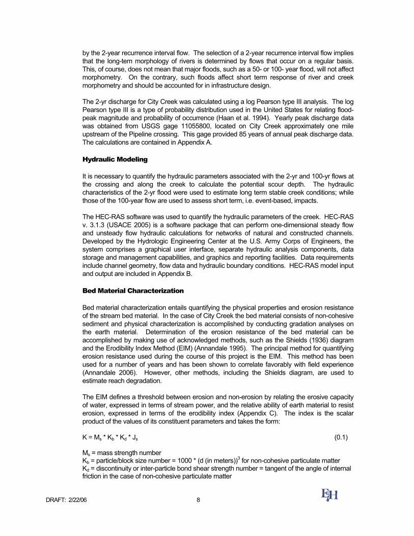
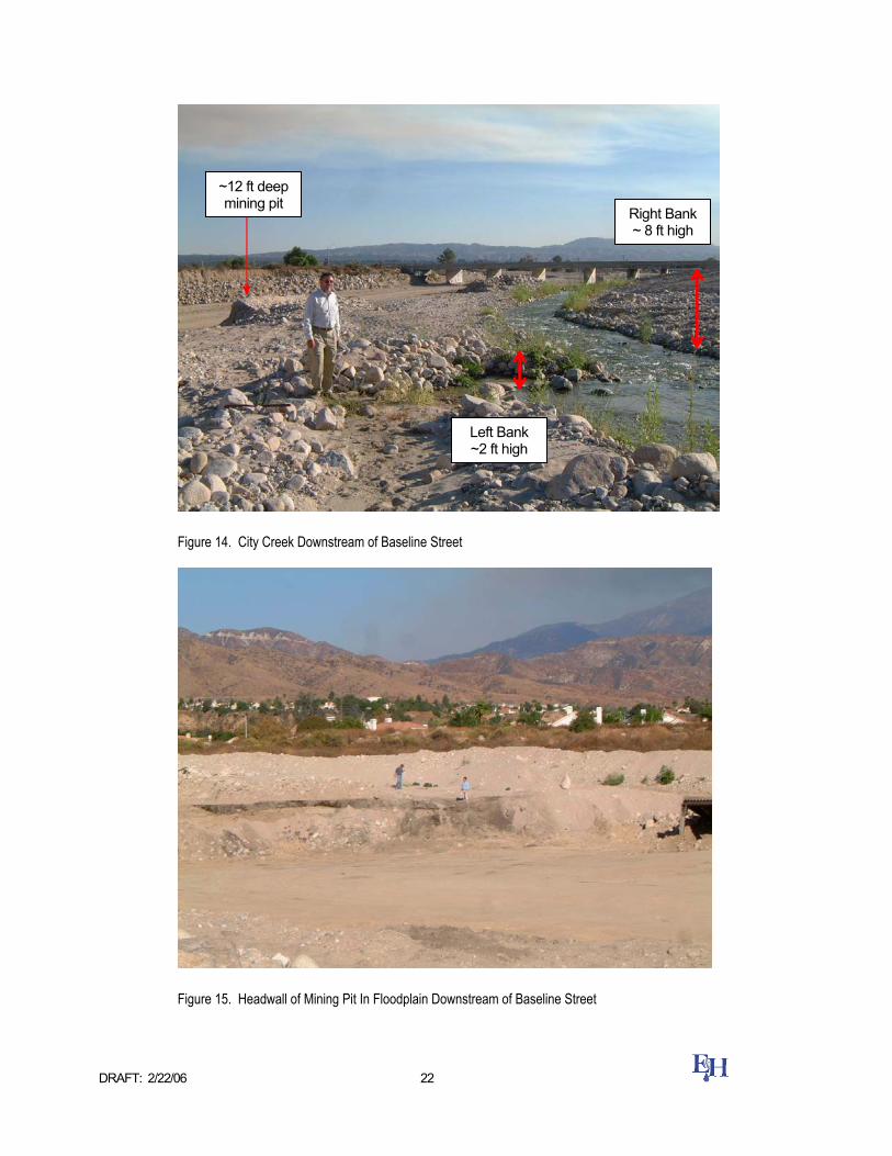
Further downstream, i.e. upstream of Boulder Avenue and downstream of Baseline Street, aggregate mining adversely impacts creek stability (Figure 14 and Figure 15). In this reach the channel flows along the right creek bank. The left bank of the small stream consists of small cobbles, about 2 feet high (Figure 14). The left floodplain has been completely excavated and currently forms a mine pit (see Figure 14 and Figure 15). If a large discharge were to flow down City Creek the presence of the pit could potentially lead to the initiation of a large headcut. The

DRAFT: 2/22/06 18
headcut could threaten Baseline Street Bridge and could potentially cause significant degradation at the Pipeline Crossing if bridge road crossing failure occurs. For purposes of this study, we assumed that any headcut associated with the pit would be arrested at Baseline Street. This position is based on the assumption that the road will be maintained and kept in good condition.
Figure 8. City Creek Exiting San Bernardino National Forest

DRAFT: 2/22/06 19
Figure 9. City Creek Entering Santa Ana River
Figure 10. Photo of the Pipeline Crossing (Upstream is on the Right)
Santa Ana River
City Creek
Approximate location of
pipeline crossing

DRAFT: 2/22/06 20
Figure 11. City Creek at Highland Ave Looking Downstream
Figure 12. Channelization of City Creek (Base Line St and Boulder Ave in Background), Looking Downstream

DRAFT: 2/22/06 21
Sant
a An
aSan Bernardino National Forest
Hig
hlan
d
Bas
e Li
ne
ErosionSediment Transport (erosion/deposition)Sediment Transport (deposition)Deposition
Sant
a An
aSan Bernardino National Forest
Hig
hlan
d
Base
Lin
e
Sant
a An
aSan Bernardino National Forest
Hig
hlan
d
Base
Lin
e
Conditions Identified in 1995
Conditions Identified in 2005
Future Conditions: No Man-Made Influence
Channelizing the stream has moved the erosional and depositional zones farther downstream. The slope will becomesteeper in the area of interest.
The deposition in downstream reachestranslates into a decrease in slope. Depositionwill start migrating upstream. Through geologic time, the stream channel will return to the equilibrium conditions identified in 1995. In the near future, the Inland Feeder Pipeline is in danger of being exposed.
Sant
a An
aSa
nta
AnaSan Bernardino
National ForestSan Bernardino National Forest
Hig
hlan
d
Bas
e Li
ne
ErosionSediment Transport (erosion/deposition)Sediment Transport (deposition)Deposition
ErosionSediment Transport (erosion/deposition)Sediment Transport (deposition)Deposition
Sant
a An
aSa
nta
AnaSan Bernardino
National ForestSan Bernardino National Forest
Hig
hlan
d
Base
Lin
e
Sant
a An
aSa
nta
AnaSan Bernardino
National ForestSan Bernardino National Forest
Hig
hlan
d
Base
Lin
e
Conditions Identified in 1995
Conditions Identified in 2005
Future Conditions: No Man-Made Influence
Channelizing the stream has moved the erosional and depositional zones farther downstream. The slope will becomesteeper in the area of interest.
The deposition in downstream reachestranslates into a decrease in slope. Depositionwill start migrating upstream. Through geologic time, the stream channel will return to the equilibrium conditions identified in 1995. In the near future, the Inland Feeder Pipeline is in danger of being exposed.
Figure 13. Schematic of Historic, Current, and Possible Future Geomorphic Conditions of City Creek
DRAFT: 2/22/06 22
Figure 14. City Creek Downstream of Baseline Street
Figure 15. Headwall of Mining Pit In Floodplain Downstream of Baseline Street
Right Bank ~ 8 ft high
Left Bank ~2 ft high
~12 ft deep mining pit

DRAFT: 2/22/06 23
Existing Topography
The site topography was obtained from drawings provided by MWD (Plate 1). The current average longitudinal slope of the creek is 0.027 ft/ft, while that in the vicinity of the pipe crossing is 0.039 ft/ft. The longitudinal profile of the main thalweg (Figure 16) illustrates the presence of headcuts throughout the reach. Most of these headcuts are actively migrating upstream.

DRAFT: 2/22/06 24
1250
1300
1350
1400
1450
1500
0 1000 2000 3000 4000 5000 6000 7000 8000 9000 10000
Station (ft)
Elev
atio
n (ft
)Thalweg ProfileHighland Ave.Inland Feeder PipelineBaseline St.Boulder Ave.8 ft headcut
5 ft headcut
4 ft headcut
5 ft headcut
4 ft headcut
4 ft headcut
Figure 16. City Creek Longitudinal Profile Indicating Head Cut Locations

DRAFT: 2/22/06 25
Figure 17. Photograph of City Creek in 2003
Figure. 18 Photograph of City Creek in 2005
Historical Morphologic Analysis
E&H did not conduct a full investigation into the historical morphology of the channel. The reason for this is that the recent alterations to the channel are deemed to have a more substantial impact on the hydraulics and sediment transport of the creek than what historical trends would show. This is readily apparent when comparing Figure 17 and Figure. 18. The removal of vegetation significantly increased the erosion potential of the channel, as did the channelization imposed on the creek.
Pipeline Crossing
Pipeline Crossing

DRAFT: 2/22/06 26
Hydrology
The majority of the hydrologic data required for the analysis, i.e. the flood peak estimates for the10-yr 24-hr, 50-yr 24-hr,,100-yr 3-hr, 100-yr 24-hr, and the Standard Project Flood are contained in the report by Chang (1995). Additionally, an estimate of the 2-yr recurrence interval flood, i.e. the assumed dominant flow, is also required for estimating stable creek conditions.
To estimate the magnitude of the 2-yr storm, the yearly peak discharge data was obtained from USGS gage 11055800 located on City Creek approximately one mile upstream of the Pipeline crossing (Figure 19). This gage provided 85 years of annual peak discharges. Using a log Pearson type III distribution, the 2-yr flood peak was calculated as 400 cfs (see Appendix A). The flood peak discharges obtained with the statistical analysis are compared with those from Chang (1995) – see Table 2. The highlighted discharges were used for analyzing scour in order to be consistent with previous studies.
Table 2. City Creek Flood Peak Discharges
Log Pearson III Chang (1995)
Recurrence Discharge (cfs) Discharge (cfs) Standard Project Flood N/A 15000
100-yr (24-hr storm) 8548 10500 100-yr (3-hr storm) N/A 13000
50-yr 5983 6600 25-yr 4021 N/A 10-yr 2174 2150 5-yr 1221 N/A 2-yr 400 N/A
1.0101-yr 19 N/A

DRAFT: 2/22/06 27
Figure 19. Location of USGS Stream Flow Gage 11055800
Hydraulics
The hydraulic parameters required for conducting the reach and local scour analysis were calculated by making use of a HEC-RAS model. The primary HEC-RAS model represents existing conditions (EXST). Additionally, three other HEC-RAS models to simulate construction of a trapezoidal channel with varying channel bottom widths of 50 ft (ALT50), 70 ft (ALT 70), and 100 ft (ALT100) were also developed. The results from these three models were used to evaluate potential design alternatives (see DESIGN ALTERNATIVES section). The cross-section for all four models at the pipeline crossing is shown on Figure 20. A steady-state solution procedure was used to simulate flow in the creek using the highlighted discharges in Table 2. The model information is included in Appendix C and results are summarized on Figure 21 - Figure 23.
USGS Gage 11055800

DRAFT: 2/22/06 28
1425
1430
1435
1440
1445
1450
1455
1460
-50 0 50 100 150 200 250 300
Station (ft)
Elev
atio
n (ft
)
EXST ALT50 ALT70 ALT100
Figure 20. Pipeline Cross-sections Used for the HEC-RAS Models
0
5
10
15
20
25
30
35
40
45
50
EXST ALT50 ALT70 ALT100
HEC-RAS Model Name
Velo
city
(ft/s
)
2-yr10-yr50-yr100-yr 24-hr100-yr 3-hrFlood
Figure 21. Average Flow Velocities at Pipeline Crossing (Calculated with HEC-RAS)

DRAFT: 2/22/06 29
0
5
10
15
20
25
EXST ALT50 ALT70 ALT100
HEC-RAS Model Name
Shea
r Str
ess
(lbf/f
t2 )2-yr10-yr50-yr100-yr 24-hr100-yr 3-hrFlood
Figure 22. Shear Stress at Channel Bottom at Pipeline Crossing (Calculated with HEC-RAS)
0
2
4
6
8
10
12
14
16
EXST ALT50 ALT70 ALT100
HEC-RAS Model Name
Stre
am P
ower
(kW
/m2 )
2-yr10-yr50-yr100-yr 24-hr100-yr 3-hrFlood
Figure 23. Stream Power at Channel Bottom at pipeline crossing (Calculated with HEC-RAS)

DRAFT: 2/22/06 30
Material Characterization
Bed Material Gradation
The bed material gradation (Figure 24) for City Creek was obtained from Chang (1995). We found no reason to believe that the essential character of the bed material in City Creek changed since 1995 and therefore used the same gradation for execution of our study.
0.01 0.1 1 10 100 1 .103 1 .1040
10
20
30
40
50
60
70
80
90
100
Screen size, mm
Perc
ent f
iner
Figure 24. Bed Material Gradation (Chang 1995)
Erosion Resistance
The erosion resistance of bed material was estimated for both the median bed material particle size and the median armor layer particle size. The median particle size is determined as 25mm from Figure 24. The armor layer particle size range is estimated between 125mm and 435mm for dominant flow conditions at the pipeline crossing and other locations upstream of the Baseline Street Crossing. These are the armor layer sizes that are anticipated to develop over the long term. The erosion threshold stream powers for these particle sizes are shown in Table 3.
Table 3. Threshold Stream Power at Pipeline Crossing
Material Type
Median Size (mm)
Threshold Stream Power (W/m2)
Bed material 25 15.5 Armor Layer (small) 125 181 Armor Layer (large) 435 3250

DRAFT: 2/22/06 31
Scour Analysis
Reach Degradation
Armor Layer Formation
The hydraulic parameters for the 2-yr discharge in the EXST, ALT50, ALT70 and ALT100 HEC-RAS models were used to determine if an armor layer will form at the pipeline crossing and, if so, how much scour will occur until its complete formation. Table 4 summarizes the results of the analysis conducted at the pipeline crossing using the Meyer-Peter Muller; Competent Bottom Velocity; Lane’s Tractive Force; Shields Diagram; Yang Incipient Motion, and Gessler methods.
Figure 25 compares the median armor layer diameter at the pipeline crossing with the original bed material gradation. This comparison indicates that it is possible for an armor layer to form from this bed material. All the calculated sizes are associated with percentage passing values indicating that 10% or more of the bed material is equal to or greater than the calculated particle size. This satisfies Pemberton and Lara’s (1984) criterion.
Once the armor layer sizes were determined, the scour depth that will occur prior to formation of the armor layer was calculated using equation (0.2). Example calculations are presented in Appendix D and results at the pipeline are also summarized in Table 4.
Table 4 indicates that the median diameter of the armor layer can be as much as 17 in (435mm), with an associated scour depth prior to formation of 23 ft (7 m). Should it be possible to widen the channel and maintain this configuration when water discharges through the section, the armor layer diameter that will develop can be as small as 6 in (150 mm) and an associated scour depth of about 4 ft (1.2 m). Implementation of such widening should be conducted with care. If not implemented correctly, the same scenario found during the 2004 / 2005 floods will occur, i.e. deepening of the channel by low flow incisement. This will concentrate the flow, as is currently the case, essentially reverting back to current conditions.
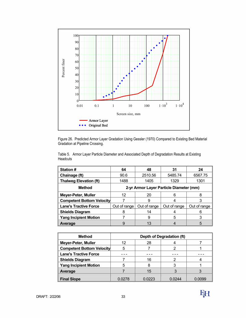
Figure 26 shows the predicted armor layer gradation using the Gessler (1970) approach for existing conditions. It is compared with the stream bed material gradation curve and shows that the particle sizes required for armor layer formation are present in the virgin material.
In addition to investigating armoring at the pipeline crossing, he bed degradation subject to formation of an armor layer has also been calculated at four existing headcuts, located at stations 64, 48, 31, and 24 in the EXST HEC-RAS model, using the hydraulic parameters for the 2-yr discharge from the EXST model. The armor layer median size and associated depth of degradation for these locations can be seen in Table 4. Figure 27 indicates an increase in scour depth associated with armor layer formation in the upstream reaches, and lower values just upstream of the Baseline Street crossing. The reason for this is that the erosive capacity of the water in the vicinity of the pipeline is greater due to flow concentration in the incised channel, while damming of flow upstream of the Baseline Street bridge results in lower stream power, and therefore smaller armor layer size requirements to maintain channel bed stability.

DRAFT: 2/22/06 32
Table 4. Armor Layer Particle Diameter and Associated Depth of Degradation Results at the Pipeline Crossing
Armor Layer Particle Diameter (in) Method EXST ALT50 ALT70 ALT100
Meyer-Peter, Muller 20 10 9 7 Competent Bottom Velocity 15 7.5 6 4 Lane's Tractive Force Out of range 4 4 4 Shields Diagram 14 7 6 5 Yang Incipient Motion 16 8 6 5 Gessler D50 20 16 13 12 Average Particle Diameter 17 9 7 6
Depth of Degradation (ft)
Method EXST ALT50 ALT70 ALT100 Meyer-Peter, Muller 28 9 7 5 Competent Bottom Velocity 18 6 4 2 Lane's Tractive Force - - - 2 2 2 Shields Diagram 16 5 5 3 Yang Incipient Motion 21 6 4 3 Gessler D50 29 8 6 4 Average Depth of Degradation 23 8 6 4
0
10
20
30
40
50
60
70
80
90
100
0.001 0.01 0.1 1 10 100
Grain Size, in
Perc
ent P
assi
ng
GSD @ Highland Avenue EXST ALT50 ALT70 ALT100
Figure 25. Existing Grain Size Distribution and Calculated Armor Layer D50 for All Four Geometries Evaluated
DRAFT: 2/22/06 33
0.01 0.1 1 10 100 1 .103 1 .1040
10
20
30
40
50
60
70
80
90
100
Armor LayerOriginal BedArmor LayerOriginal Bed
Screen size, mm
Perc
ent f
iner
Figure 26. Predicted Armor Layer Gradation Using Gessler (1970) Compared to Existing Bed Material Gradation at Pipeline Crossing.
Table 5. Armor Layer Particle Diameter and Associated Depth of Degradation Results at Existing Headcuts
Station # 64 48 31 24 Chainage (ft) 90.6 2510.56 5485.74 6567.75 Thalweg Elevation (ft) 1488 1405 1329 1301
Method 2-yr Armor Layer Particle Diameter (mm)
Meyer-Peter, Muller 12 20 6 8 Competent Bottom Velocity 7 9 4 3 Lane's Tractive Force Out of range Out of range Out of range Out of range Shields Diagram 8 14 4 6 Yang Incipient Motion 7 9 5 3 Average 9 13 4 5
Method Depth of Degradation (ft)
Meyer-Peter, Muller 12 28 4 7 Competent Bottom Velocity 5 7 2 1 Lane's Tractive Force - - - - - - - - - - - - Shields Diagram 7 16 2 4 Yang Incipient Motion 5 8 3 1 Average 7 15 3 3
Final Slope 0.0278 0.0223 0.0244 0.0099

DRAFT: 2/22/06 34
1250
1300
1350
1400
1450
1500
0 1000 2000 3000 4000 5000 6000 7000 8000 9000 10000
Station (ft)
Elev
atio
n (ft
)Thalweg Profile
Highland Ave.
Inland Feeder Pipeline
Baseline St.
~ Pipe Elev.
'Armor Layer Stable Slopes'
Figure 27. Estimated Scour Depths Associated With Armor Layer Formation

DRAFT: 2/22/06 35
Stable Longitudinal Stream Slope associated with Median Particle Size
The potential for armor layer formation in City Creek indicates that the quasi-equilibrium creek slope will be subject to the formation of such a layer. Nevertheless, the stable slopes associated with the median grain size of the original bed material have been calculated in order to be complete.
The stable slope associated with the median particle size of the original bed gradation is likely to be much milder than that associated with the armor layer. The scour at the Pipeline, should stable slope conditions associated with the median particle size govern, is calculated by pivoting a line around the baselevel at the Baseline Street culvert. The relevant elevations and distances used in such a calculation are shown in Table 6. The estimated stable channel slopes for these conditions are presented in Table 7.
Table 6. Base Level Information and Estimated Time for Stable Conditions to Establish if Median Bed Material Particle Size Dominates in the Determination of Quasi-Equilibrium Conditions
Grade Control Structure Location: Baseline St. Culvert Elevation of Thalweg of Baseline St. Culvert: 1296 ft Distance Between Pipeline and Baseline St.: 4947.18 ft Current Thalweg Elevation at Pipeline Crossing: 1430 ft Estimated Time for Stable Conditions to establish 100 yr
Table 7. Estimated Stable Slope, Depth of Degradation, and Rate of Scour at Pipeline Crossing Assuming Median Bed Material Diameter Control
Bottom Width (ft) EXST ALT50 ALT70 ALT100 Scholitsch 0.18% 0.41% 0.53% 0.69%
Meyer-Peter, Muller 0.22% 0.60% 0.73% 0.88% Shields Diagram 0.30% 0.84% 1.00% 1.30%
Lane's Tractive Force 0.31% 0.87% 1.10% 1.30%
Stab
le S
lope
Average 0.26% 0.68% 0.84% 1.00% Scholitsch 125 114 108 100
Meyer-Peter, Muller 123 104 98 91 Shields Diagram 119 92 85 70
Lane's Tractive Force 119 91 80 70
Deg
rada
tion
@ P
ipel
ine
(ft)
Average 121 100 93 85 Average Scour Per Year (ft/yr)* 1.21 1.00 0.93 0.85
*Assumes 100 years for full degradation depth
Although the total depth of degradation at the pipeline crossing for this method was calculated to be 121 ft, this is not the predicted total depth of erosion due to the presence of coarse material in the bed and the potential for armor layer formation.
Net Reach Degradation
The net amount of scour, in the absence of human intervention, at the pipeline crossing is controlled by an armor layer formation, if the necessary particle gradations are present in

DRAFT: 2/22/06 36
the bed material, or the median particle size slope, if coarse materials are not present. The reason for this is that once the stable condition has established at a certain elevation in the stream bed, it is assumed not to degrade any further.
The estimated reach degradation depth at the pipeline crossing is therefore 23ft below the current bed elevation at the pipeline crossing assuming that armoring occurs (Table 4).
Local Scour
Bend Scour
Figure 28 shows the bend in current existence in the vicinity of the pipeline crossing. The additional scour that could occur as a result of flow around this bend was estimated for dominant flow conditions using the procedures outlined before for existing conditions. This entails calculating the total stream power around the bend and comparing it with the erosion resistance of the bed and bank material. If this comparison indicates scour potential, the next step is to calculate the additional scour depth around the bend resulting from bend flow.
Using the procedure by Chang (1992) for existing conditions and the 2-year recurrence interval discharge it is found that the maximum total stream power around the bend is 1470 W/m2. A comparison between earth material erosion resistance and the maximum stream power around the bend is provided in Table 8. This comparison indicates that it is possible for the stream bed material to erode prior to and after the formation of an armor layer.
The scour depth around the bend was estimated using the Odgaard (1986) three-dimensional analytical model. The result of the calculation is shown on Figure 29. Estimated scour depth, in addition to what would occur without the bend, is about 0.5m (18 inches).
Table 8. Comparison Between Stream Power in Bend and Erosion Threshold.
Material Type Erosion
Threshold (W/m2)
Total Stream Power around Bend (W/m2)
Erosion? (Yes / No)
Original Bed Material 15.2 1470 Yes Armor Layer 944 1470 Yes

DRAFT: 2/22/06 37
Figure 28. Location and Dimensions of Bend Analyzed
Figure 29. Three-Dimensional Image of Calculated Bend Scour at the Pipeline Crossing.

DRAFT: 2/22/06 38
Headcut Migration
Headcuts were noted during the field visit. Headcut migration is a long term scour mechanism that over time aids in achieving equilibrium in the channel, at which time the channel bed will be armored. To illustrate that the current headcut will migrate upstream, we calculated the erosive capacity of the backroller at the base of the headcut drop and compared it with the threshold stream power of the base material. The results for the seven headcuts observed on site are presented in Table 9. The table illustrates that the stream power associated with the back roller is higher than the erosion threshold of the existing bed materials and that the headcuts will migrate upstream.
Table 9. Backroller Stream Power Associated with Active Headcuts
Stream Power (W/m2) Drop Height (ft) Back Roller Threshold
64 4 2280 15.2 57 3 749 15.2 56 6 1989 15.2 48 5 2589 15.2 35 4 1300 15.2 31 4 1077 15.2 24 3 620 15.2
SUMMARY
It is concluded that the scour in City Creek will continue in the future in the absence of intervention. The scour process will be aided by headcut migration, and will stabilize once an armor layer has formed throughout the reach. This results in approximately 23ft of scour at the pipeline crossing, below the current elevation. It was found that bend scour at the pipeline crossing is on the order of about 18 inches, which makes the total predicted depth of erosion at the Pipeline to be 25ft.
It has also been shown that degradation of the river reach will continue even if the cross section is widened quite substantially. In order to mitigate the scour at the pipeline, the essential design approach should be to make the slope milder, while concurrently widening the channel section. Re-vegetation of the channel bed and banks will assist in further stabilizing the reach.
DESIGN ALTERNATIVES
The approach to the design of mitigation measures is based on the insight we developed during the course of the analysis. Our interpretation of the fluvial geomorphic nature of the reach indicates that it is possible for it to return to a depositional zone in the very long term (geologic time). However, in following the course to reverting back to a depositional zone, our analysis indicates that scour up to a maximum depth of about 23ft below current thalweg elevations will first occur. It is therefore necessary to protect the pipeline against the consequences of such an event. For design purposes we ignore the geologic time

DRAFT: 2/22/06 39
scenario, i.e. the area eventually reverting back to a depositional zone. However, this insight is used to conceptualize a stable mitigation design.
The focus of the mitigation design approach should be to provide a design configuration that will accelerate the geomorphic process to revert the river reach containing the pipeline crossing back to a depositional zone. In principal this can be accomplished by designing mitigation elements that will reduce the river slope and prevent occurrence of low-flow channel incision.
The recommended design flood equals the 100-year, 3-hr design discharge. Should MWD require implementation of the Standard Project Flood, this discharge should replace our recommendation. The discharge for designing mitigation measures is considerably larger than the discharge used to estimate long term quasi-equilibrium conditions. This is for obvious reasons. When assessing long-term stability, it is appropriate to use the associated dominant discharge. However, for protection, it is necessary to use a large design flood, with an appropriate probability of occurrence to protect infrastructure and public safety.
The table below lists optional mitigation strategies and indicates our assessment of anticipated feasibility. A description of each measure is provided below the table. It should be noted that E&H’s commission was to recommend potential mitigation measures in a conceptual manner. However, we have conducted preliminary analyses to identify potential fatal flaws. Exact sizing of structures can be accomplished once a preferred solution has been selected.

DRAFT: 2/22/06 40
Table 10. Optional Mitigation Measures
Mitigation Measure Feasible? (Yes / No) Comment
Channel Widening; without boundary hardening
No The current situation developed after a widened channel was created to pass a flood. The inability of a non-hardened widened channel bed to resist the erosive capacity of water led to the development of an incised channel. This is confirmed by comparing the erosive capacity of the water flowing for design flow conditions in wide channels to the erosion resistance of the bed material, even after armoring has occurred. The comparison indicates that the channel bottom will scour.
Riprap Chute Yes A riprap chute terminating in a riprap energy dissipater basin can be used to guide flows to lower elevations below the pipeline crossing. Feasible rock sizes are obtained when the chute is about 200ft to 250ft wide, with a slope of about 1V:5H. Rock sizes are roughly ½ ton rock.
Single Vertical Drop Structure
No A structure consisting of a single, vertical drop is not considered be feasible. The drop height is anticipated to be too high. It poses engineering and construction problems, and is a potential public safety hazard.
Multiple Drops Yes Multiple drops, using a concept similar to the riprap chute is considered feasible. It adds redundancy and diminishes public safety concerns. Multiple drops using vertical walls (concrete or sheet piling) is considered less desirable from an engineering and construction, and public safety points of view.

DRAFT: 2/22/06 41
Channel Widening without Boundary Hardening
It is not considered feasible to propose a concrete-lined channel to protect the pipeline against the effects of scour. This alternative mitigation design therefore entails widening the channel without boundary hardening.
Ideally, if flow is spread over a wider channel the erosive capacity of the water per unit area of the bed is expected to decrease. A comparison of the applied stream power to the channel bed during design flood conditions and the threshold stream power of an armor layer associated with a 100 ft wide channel is presented in Table 11. The comparison indicates that the channel bottom is likely to scour. Experience during the 2004 / 2005 floods indicate that this is a reasonable expectation. The bed of the trapezoidal channel that was created scoured and was incised. Channel widening without hardening of the boundary is not considered a feasible solution to the scour problem.
Table 11. Comparison of Erosive Capacity of Water for Design Flood Conditions and the Threshold Stream Power of an Armor Layer that is Expected to Form Under Such Conditions.
Erosive Capacity of SPF in ALT100 Armored Channel 12.3 kW/m2 Erosive Threshold of Armor Layer for ALT100 0.24 kW/m2
Riprap Chute
This mitigation design entails filling the area above and upstream of the pipeline crossing to create a mild slope and force a depositional area. The milder sloped channel reach terminates in a riprap-lined chute, which guides the water to a lower elevation to meet the thalweg of the downstream channel. The riprap in the chute protects the pipeline and the underlying earth material against scour. The mild slope upstream of the riprap chute forces deposition of sediment, and prevents formation of an incised channel. Chute slopes of 20% or less can feasibly be protected against scour with approximately ½ ton rock. This might be a feasible solution provided adequate availability of rock. The rirprap rock size will be confirmed and more design detail provided if a decision is made to implement this potential design solution.

DRAFT: 2/22/06 42
Figure 30. Conceptual Configuration of Riprap Lined Rock Chute. Exact Dimensions to be Determined During Preliminary and Final Design.
Single Vertical Drop Structure
The essential concept when implementing a single drop structure is to create a mild channel slope upstream of the drop structure by backfilling, establish sub-critical flow conditions, force deposition of sediment in the reach upstream of the drop, and prevent formation of an incised channel in this sub-reach of the channel. Our opinion is that the vertical drop associated with such a structure will be too great. This presents the designer with hydraulic, geotechnical and structural design problems that might be difficult to overcome, in addition to public safety concerns (Figure 31). Design details to facilitate construction of such a structure need resolving.
Figure 31. Conceptual Sketch of Single Drop Structure.
Fill
Mild slope and depositional zone
Mild Slope and depositional zone

DRAFT: 2/22/06 43
Multiple Grade Control Structures
The implementation of multiple grade control structures is a design mitigation approach with merit. Two optional approaches can be followed. The drop structures can be constructed of a hard material, i.e. vertical concrete walls or sheet piling; or it can be constructed of riprap, similar to the riprap design chute.
If a vertical drop structure is constructed E&H recommends against using drops in excess of 3ft. Such a design will require a large number of drop structures; approximately 20 to 40, depending on layout detail and is most probably not feasible.
Implementation of this concept becomes more feasible when using riprap chutes (Figure 32). The reason for this is that the individual drops that can be accommodated are greater than when using a vertical drop. As the water flows down the inclined slopes of these structures, it dissipates energy on a continuous basis.
A potential benefit of using multiple grade control structures is that they may exhibit greater overall stability. For example, if one of the structures fails the other may be assist in preventing overall failure. Such a system is characterized by increased redundancy, making is safer. Additionally, the use of smaller drops reduces public safety concerns.
Figure 32. Multiple Rock Chutes.
Mild Slope and Depositional Zone
Multiple Rock Chutes

DRAFT: 2/22/06 44
REFERENCES
Annable, W.K. 1994. Morphological relations of rural water courses in southeastern Ontario for use in natural channel design, Masters thesis, Univ. of Guelph, School of Engineering, Guelph, Ontario, Canada.
Andrews, E.D. 1980. Effective and bankfull discharges of streams in the Yampa River Basin,
Colorado and Wyoming, Journal of Hydrology, 46: 311-330. Annandale, G.W. 2006. Scour Technology, McGraw-Hill, New York. Annandale, G.W. 1995. Erodibility. Journal of Hydraulic Research 33:471-494. Chamani, M.R. and M.K. Beirami. “Flow Characteristics at Drops” Journal of Hydraulic
Engineering, 128(8), 2002.
Chang, Howard H. 1992. Fluvial Processes in River Engineering. Krieger Publishing Company. Malabar, Florida.
Chang, Howard H. 1995. Inland Feeder Pipeline, San Bernardino Segment (Contract 3):
Fluvial Study of City Creek for Pipeline Placement. Prepared for Dames and Moore. Gessler, J. 1971. Beginning & Ceasing of Sediment Motion.” River Mechanics, H.W. Shen,
ed Hseieh Wen Shen, Fort Collins, Colorado, 7, 1-22.
Google Earth 2006. [Google Earth version 3.0.0762] 34º 07’ 40.87” N, 117 º 11’ 20.50” W
Haan C.T., B. J. Barfield, and J.C. Hayes. 1994. Design hydrology and sedimentology for small catchments. San Diego CA : Academic Press Inc.
Haestad Methods, Inc. 2003. FlowMaster v.6.1 [computer software]. www.haestad.com. Lane, E.W. 1955. The importance of fluvial morphology in hydraulic engineering. American
Society of Engineering, Proceedings. 81. Paper 745: 1-17. Leopold, Luna B. 1994. A View of the River. Cambridge, Massachusetts: Harvard University
Press. Odgaard, A.J., "Meander Flow Model Parts I and II", Journal of Hydraulic Engineering, Vol.
112, No. 12, December 1986, ASCE, pp. 1117-1150. Pemberton, EL and JM Lara. 1984. Computing Degradation and Local Scour. Technical
Guideline for Bureau of Reclamation. Denver, Colorado. Rosgen, David L. 1996. Applied river morphology. Pagosa Springs, CO : Wildland Hydrology. U.S. Army Corps of Engineers (USACE). 2001. HEC-RAS River Analysis System v. 3.3.1
[computer software]. www.hec.usace.army.mil. USGS, 2006 Gage 11055800 Annual Peak Streamflow Data for period of record.
http://nwis.waterdata.usgs.gov/nwis/peaks/?site_no=11055800&agency_cd=USGS.

DRAFT: 2/22/06 45

APPENDIX A – HYDROLOGY CALCULATIONS

DRAFT 2/22/2006 A-1
Appendix A: HYDROLOGY
Objective
In the Chang Study (1995) provided by the Metropolitan Water District (MWD), a hydrologic study of the watershed was performed and the following recurrence interval discharges were reported: 10-year 24-hour, 50-year 24-hour, 100-year 3-hour, 100-year 24-hour, and the project flood. Although these discharges were used in our study, the discharge of interest in estimating the stability of the channel is the dominant discharge, in this case the two-year recurrence interval discharge.
In order to evaluate the two-year discharge, yearly peak discharge data was obtained form USGS gage 11055800 (2005) and analyzed using a Log Pearson III distribution (Haan & Barfield, 1994). The results of the Log Pearson III distribution were compared to the reported discharges in the Chang Study.
Assumptions
• All discharges reported in by Chang (1995) are considered accurate;
• There are no trends in the data;
• The data represent independent hydrologic events;
• The flows are from a single population; and
• Measurement errors are random, unbiased, and have a relatively small variance.
Calculations
To estimate the magnitude of the two-year storm and verify the values reported by Chang (1995), the yearly peak discharge data was obtained form USGS gage 11055800 located on City Creek approximately one mile upstream of the Inland Feeder Pipeline crossing (Figure A-1). This gage provided 85 years of historical annual peak discharge data (Table A-1).
Figure A-1: Location of USGS Streamflow Gage 11055800
USGS Gage 11055800

DRAFT 2/22/2006 A-2
Table A-1: Historical Annual Peak Discharge from USGS Gage 11055800
Year Peak Discharge (cfs) Year Peak Discharge
(cfs)
1920 350 1963 163 1921 1320 1964 64 1922 1090 1965 292 1923 720 1966 1310 1924 345 1967 3080 1925 74 1968 217 1926 2360 1969 7000 1927 1930 1970 205 1928 369 1971 100 1929 196 1972 722 1930 78 1973 492 1931 146 1974 126 1932 442 1975 103 1933 62 1976 326 1934 374 1977 860 1935 166 1978 2510 1936 580 1979 359 1937 1500 1980 3630 1938 6900 1981 103 1939 400 1982 330 1940 378 1983 1140 1941 2420 1984 287 1942 172 1985 200 1943 2300 1986 530 1944 1030 1987 108 1945 940 1988 108 1946 1000 1989 262 1947 285 1990 175 1948 250 1991 460 1949 100 1992 853 1950 198 1993 1910 1951 71 1994 188 1952 937 1995 2260 1953 132 1996 445 1954 631 1997 1360 1955 115 1998 2210 1956 862 1999 37 1957 1650 2000 162 1958 1350 2001 105 1959 358 2002 8.7 1960 42 2003 272 1961 92 2004 8000 1962 648

DRAFT 2/22/2006 A-3
It is possible to estimate the magnitude of discharges for various recurrence intervals by fitting the data to a particular probability distribution. Four commonly used distributions are the following: Normal, Lognormal, Extreme Value 1, and Log Pearson III. Skewness, a measure of the symmetry of the data, is a good parameter to determine the best probability distribution to fit the data and the equation to calculate skewness can be seen below:
( )
( )( )
3
31 2i
sx
n X XC
n n S−
=− −∑
. (A.1)
The skewness of the raw data set was calculated to be 3.3. Table A-2 provides the optimal skewness values for each probability distribution. To test the appropriateness of the Lognormal distribution, the coefficient of variance, vC , must be determined:
xvSCX
= (A.2)
where xS is the standard deviation 2 2i
x
X nXS
n 1
− = −
∑ and X is the mean iXXn
= ∑ .
vC was calculated to be 1.57 and according to Table A-2 the appropriate skewness for the
Lognormal distribution should be close to 33 v vC C+ , which in this case is equal to 8.64.
Due to the magnitude of the skewness, the most appropriate probability distribution is the Log Pearson III (LPIII). The LPIII is capable of handling any skewness values a data set yields.
Table A-2 Appropriate Skewness Values for Possible Probability Distributions
Distribution SkewnessNormal 0Lognormal 33 v vC C+Extreme Value I 1.139Log Pearson III Any value
Following are the steps involved in using the LPIII distribution:
1. transform the n original observations, iX , to logarithmic values, iY , by the relation
i iY logX= ; (A.3)
2. compute the mean logarithm, Y
iYYn
=∑; (A.4)
3. compute the standard deviation of the logarithm, YS

DRAFT 2/22/2006 A-4
2 2i
y
Y nYS
n 1−
=−
∑ ; (A.5)
4. compute the coefficient of skewness SC from
( )( )( )
3
31 2i
sY
n Y YC
n n S−
=− −∑
; (A.6)
5. compute
T Y TY Y S K= + (A.7)
where TK is from the Frequency Factors for Pearson Type III Distribution Table for all desired recurrence intervals; and
6. calculate
logT TX anti Y= (A.8)
Results
The magnitude of the 200, 100, 50, 25, 10, 5, 2, and 1.01 year discharges calculated using a LPIII distribution can be seen in Table 2 along with the 100, 50, and 10 year discharges reported in the Chang 1995 report. The discharges estimated using the LPIII distribution as well as those provided in the Chang Study are shown in Table A-3. All discharges used in our evaluation are highlighted in yellow.
Table A-3: City Creek Hydrology
Log Pearson III Dames & Moore 1995
Recurrence Discharge (cfs) Discharge (cfs) Standard Project Flood N/A 15000
100-yr (24-hr storm) 8548 10500 100-yr (3-hr storm) N/A 13000
50-yr 5983 6600 25-yr 4021 N/A 10-yr 2174 2150 5-yr 1221 N/A 2-yr 400 N/A
1.0101-yr 19 N/A

DRAFT 2/22/2006 A-5
References
Haan C.T., B. J. Barfield, and J.C. Hayes. 1994. Design Hydrology and Sedimentology for Small Catchments. San Diego CA: Academic Press Inc.
Chang, Howard H., 1995. Inland Feeder Pipeline, San Bernardino Segment (Contract 3) Fluvial Study of City Creek foe Pipeline Placement. Rancho Santa Fe CA
USGS, 2006 Gage 11055800 Annual Peak Streamflow Data for period of record. http://nwis.waterdata.usgs.gov/nwis/peaks/?site_no=11055800&agency_cd=USGS.

APPENDIX B – HEC-RAS MODEL

DRAFT 2/22/2006 B-1
Appendix B: HEC-RAS Modeling
Introduction
HEC-RAS [Version 3.1.3] was used to determine the erosive capacity of City Creek and to quantify the anticipated hydraulic characteristics at the Inland Feeder Pipeline crossing.
The primary HEC-RAS model represents existing conditions (EXST). In addition to evaluating the hydraulic parameters for the existing conditions, three alternative HEC-RAS models were constructed to simulate construction of a trapezoidal channel with channel bottom widths of 50 ft (ALT50), 70 ft (ALT 70), or 100 ft (ALT100). All models were run in steady state. The cross-section for the pipeline crossing for all four models can be seen in Figure B-2.
Assumptions
General assumptions made for this model were:
• One Dimensional Flow: The system of equations used to solve the hydraulics of the channel in HEC-RAS only takes into account one dimensional flow. The hydraulics around the structures can be two and three dimensional.
• Hydrology: The magnitude of the 10-year, 50-year, 100-year 3-hour, 100-year 24-hour, and Standard Project Flood developed in Chang (1995) is assumed to still be valid for this site. This is a reasonable assumption as the creek discharges directly from the San Bernardino forest and no known changes have taken place in this area since execution of the previous study by Chang (1995).

DRAFT 2/22/2006 B-2
Input
Figure B-1. Cross Section Locations for EXST, ALT50, ALT70, and ALT100
1425
1430
1435
1440
1445
1450
1455
1460
-50 0 50 100 150 200 250 300
Station (ft)
Elev
atio
n (ft
)
EXST ALT50 ALT70 ALT100
Figure B-2.: Pipeline Cross-sections Used for the HEC-RAS Models (looking upstream)
Boulder Ave.
Inland Feeder Pipeline Crossing
Highland Ave.
Baseline St.
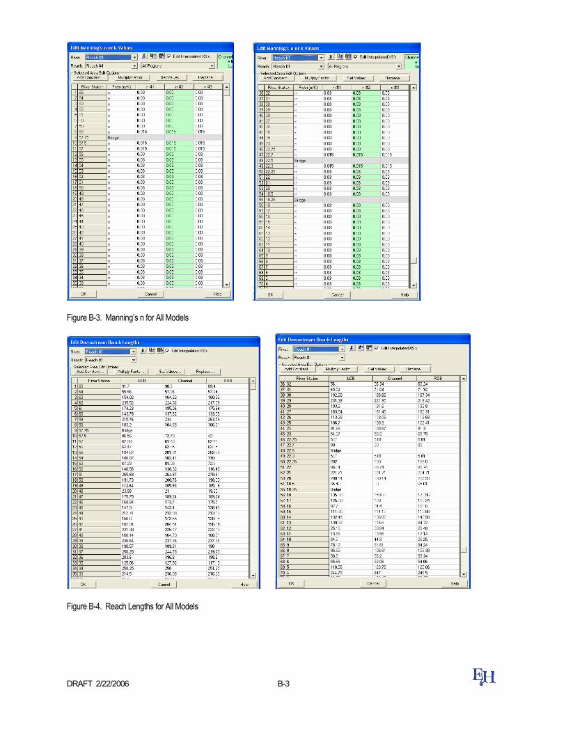
DRAFT 2/22/2006 B-3
Figure B-3. Manning’s n for All Models
Figure B-4. Reach Lengths for All Models

DRAFT 2/22/2006 B-4
Figure B-5. Contraction/Expansion Coefficients for All Models
Figure B-6. Bank Stations for EXST

DRAFT 2/22/2006 B-5
Figure B-7. Bank Stations for ALT50 Figure B-8. Bank Stations for ALT70
Figure B-9. Bank Stations for ALT100

DRAFT 2/22/2006 B-6
Figure B-10. Levee Stations for EXST
Figure B-11. Steady Flow Input File for All Models
Figure B-12. Boundary Condition Input File for All Models

DRAFT 2/22/2006 B-7
OUTPUTS
Overview
Figure B-13 thru Figure B-15 display the channel velocity, shear stress, and stream power for all four models (EXST, ALT50, ALT70, ALT100) for all six storm discharges.
The majority of the calculations were made using the 2-yr discharge for the various HEC-RAS models, Table B-1 thru Table B-4 display the 2-yr discharge output for the EXST, ALT50, ALT70, and ALT100 models.
0
5
10
15
20
25
30
35
40
45
50
EXST ALT50 ALT70 ALT100
HEC-RAS Model Name
Velo
city
(ft/s
)
2-yr10-yr50-yr100-yr 24-hr100-yr 3-hrFlood
Figure B-13: Flow Velocities

DRAFT 2/22/2006 B-8
0
5
10
15
20
25
EXST ALT50 ALT70 ALT100
HEC-RAS Model Name
Shea
r Str
ess
(lbf/f
t2 )
2-yr10-yr50-yr100-yr 24-hr100-yr 3-hrFlood
Figure B-14: Shear Stress at Channel Bottom
0
2
4
6
8
10
12
14
16
EXST ALT50 ALT70 ALT100
HEC-RAS Model Name
Stre
am P
ower
(kW
/m2 )
2-yr10-yr50-yr100-yr 24-hr100-yr 3-hrFlood
Figure B-15: Stream Power at Channel Bottom

DRAFT 2/22/2006 B-9
Table B-1. EXST - Existing Conditions (2-yr Storm Event) Output
HEC-RAS Plan: EXST-Final River: Reach #1 Reach: Reach #1 Profile: 2-yrRiver Sta Profile Q Total Min Ch
ElW.S. Elev
Crit W.S.
E.G. Elev
E.G. Slope
Vel Chnl
Flow Area
Top Width
Froude # Chl
Shear Chan
(cfs) (ft) (ft) (ft) (ft) (ft/ft) (ft/s) (sq ft) (ft) (lb/sq ft) (lb/ft s) (kW/m 2 )65 2-yr 400 1490 1492.08 1492.60 1493.85 0.0250 10.84 38.54 27.30 1.49 2.54 27.56 0.4064 2-yr 400 1488 1489.86 1490.33 1491.41 0.0287 10.25 41.83 39.15 1.55 2.42 24.78 0.3663 2-yr 400 1484 1485.60 1486.38 1488.34 0.0646 13.39 30.61 30.84 2.25 4.42 59.22 0.8662 2-yr 400 1480 1481.94 1482.28 1483.14 0.0261 8.96 46.85 45.45 1.45 1.93 17.30 0.2561 2-yr 400 1475 1476.89 1477.14 1477.90 0.0215 8.20 50.84 48.21 1.32 1.61 13.21 0.1960 2-yr 400 1470 1471.80 1472.09 1472.88 0.0262 8.34 47.95 45.01 1.42 1.74 14.48 0.2159 2-yr 400 1465 1466.74 1467.22 1468.33 0.0319 10.18 39.97 34.49 1.61 2.46 25.01 0.3658 2-yr 400 1462 1462.58 1462.89 1463.62 0.0149 8.37 49.79 95.81 1.94 0.54 4.48 0.07
57.75 Bridge57.5 2-yr 400 1457 1457.78 1458.39 1460.71 0.0508 13.74 29.12 60.13 3.48 1.53 21.02 0.31
57 2-yr 400 1455 1455.44 1455.87 1457.10 0.0323 10.35 38.78 88.05 2.74 0.89 9.25 0.1356 2-yr 400 1450 1451.45 1452.02 1453.22 0.0511 10.82 38.83 51.02 1.95 3.03 32.79 0.4855 2-yr 400 1444 1446.30 1447.12 1449.11 0.0674 13.47 29.92 29.17 2.27 4.51 60.74 0.8954 2-yr 400 1440 1441.50 1441.75 1442.49 0.0263 8.03 50.24 52.26 1.41 1.64 13.17 0.1953 2-yr 400 1435 1437.65 1438.12 1439.10 0.0326 9.77 42.31 41.61 1.60 2.32 22.68 0.3352 2-yr 400 1430 1432.11 1433.05 1435.13 0.0430 14.30 29.90 22.22 1.95 4.41 63.03 0.9251 2-yr 400 1425 1427.08 1427.71 1429.13 0.0383 11.48 34.83 26.35 1.76 3.08 35.41 0.5250 2-yr 400 1420 1421.82 1422.22 1423.11 0.0241 9.39 46.40 46.01 1.42 2.03 19.05 0.2849 2-yr 400 1415 1416.76 1417.15 1418.05 0.0259 9.28 45.37 43.61 1.46 2.03 18.85 0.2848 2-yr 400 1410 1412.23 1412.80 1414.04 0.0404 10.82 37.24 34.21 1.75 2.86 30.92 0.4547 2-yr 400 1405 1407.94 1409.33 1412.53 0.0629 17.20 23.26 12.32 2.21 6.40 110.01 1.6146 2-yr 400 1400 1402.84 1403.55 1405.17 0.0294 12.23 32.70 17.35 1.57 3.17 38.82 0.5745 2-yr 400 1395 1397.78 1398.32 1399.44 0.0279 10.34 38.70 26.69 1.51 2.43 25.15 0.3744 2-yr 400 1391 1392.91 1393.54 1395.00 0.0306 11.59 34.51 21.21 1.60 2.96 34.27 0.5043 2-yr 400 1385 1387.31 1387.88 1389.24 0.0257 11.12 35.96 20.66 1.49 2.66 29.60 0.4342 2-yr 400 1380 1382.24 1382.88 1384.29 0.0353 11.47 34.86 24.36 1.69 3.02 34.61 0.5041 2-yr 400 1375 1377.53 1378.14 1379.63 0.0355 12.50 38.05 39.19 1.74 3.43 42.90 0.6340 2-yr 400 1370 1372.17 1372.52 1373.45 0.0256 9.10 44.00 36.05 1.44 1.97 17.90 0.2639 2-yr 400 1365 1367.45 1368.10 1369.47 0.0278 11.98 39.51 40.67 1.56 3.03 36.34 0.5338 2-yr 400 1360 1362.23 1362.74 1363.92 0.0228 11.26 42.03 34.43 1.45 2.63 29.63 0.4337 2-yr 400 1355 1357.48 1358.05 1359.10 0.0273 10.28 40.43 35.88 1.51 2.40 24.67 0.3636 2-yr 400 1350 1351.70 1352.02 1352.83 0.0239 8.62 47.61 44.09 1.39 1.78 15.35 0.2235 2-yr 400 1345 1346.59 1347.03 1347.99 0.0366 10.58 45.86 60.59 1.71 2.69 28.50 0.4234 2-yr 400 1340 1341.99 1342.56 1343.80 0.0394 10.80 37.04 31.65 1.76 2.83 30.59 0.4533 2-yr 400 1335 1336.87 1337.14 1337.89 0.0228 8.16 50.18 47.37 1.35 1.62 13.26 0.1932 2-yr 400 1330 1331.54 1331.79 1332.51 0.0242 7.92 51.14 51.91 1.37 1.57 12.46 0.1831 2-yr 400 1329 1330.20 1330.44 1331.16 0.0213 8.17 52.20 50.25 1.31 1.60 13.04 0.1930 2-yr 400 1325 1327.24 1327.72 1328.79 0.0284 9.99 40.05 30.17 1.53 2.32 23.18 0.3429 2-yr 400 1320 1322.87 1323.16 1323.94 0.0251 8.33 48.02 43.41 1.40 1.71 14.28 0.2128 2-yr 400 1315 1316.95 1317.25 1318.03 0.0255 8.35 47.90 43.98 1.41 1.73 14.43 0.2127 2-yr 400 1310 1312.28 1312.59 1313.37 0.0234 8.39 48.06 44.23 1.37 1.70 14.29 0.2126 2-yr 400 1306 1308.14 1308.38 1309.00 0.0169 7.98 59.17 68.77 1.19 1.46 11.63 0.1725 2-yr 400 1304 1305.76 1305.90 1306.41 0.0213 6.54 62.48 76.89 1.24 1.14 7.47 0.1124 2-yr 400 1301 1302.67 1302.84 1303.40 0.0265 6.86 58.69 75.86 1.36 1.30 8.89 0.1323 2-yr 400 1297 1299.68 1299.79 1300.40 0.0184 6.83 59.18 59.48 1.18 1.18 8.03 0.12
22.75 2-yr 400 1297 1299.65 1299.89 0.0021 3.92 103.83 48.21 0.46 0.30 1.17 0.0222.7 2-yr 400 1296.83 1297.61 1298.19 1299.65 0.0197 11.47 34.88 44.99 2.30 0.92 10.56 0.1522.5 Bridge22.3 2-yr 400 1295.49 1297.82 1296.83 1298.04 0.0006 3.82 104.62 45.00 0.44 0.07 0.28 0.00
22.25 2-yr 400 1295 1297.26 1297.26 1297.97 0.0125 6.77 59.13 43.05 1.01 1.06 7.15 0.1022 2-yr 400 1291 1292.01 1292.01 1292.17 0.0025 1.75 127.67 97.30 0.40 0.09 0.16 0.0021 2-yr 400 1288 1289.53 1290.00 1291.43 0.0436 11.06 36.15 32.26 1.84 3.01 33.33 0.4920 2-yr 400 1283 1283.97 1284.00 1284.89 0.0315 7.72 51.79 62.75 1.50 1.62 12.51 0.18
18.5 2-yr 400 1273 1274.98 1274.67 1274.99 0.0002 0.81 442.34 339.81 0.13 0.02 0.01 0.0018.25 Bridge
18 2-yr 400 1273 1273.99 1273.99 1274.37 0.0147 4.93 81.12 108.69 1.01 0.68 3.37 0.0517 2-yr 400 1271 1271.51 1271.51 1271.79 0.0176 4.11 92.91 175.28 1.03 0.54 2.24 0.0316 2-yr 400 1269 1270.26 1270.00 1270.55 0.0059 4.29 94.02 82.73 0.69 0.44 1.90 0.0315 2-yr 400 1267 1269.07 1269.07 1269.74 0.0120 6.55 61.05 45.72 1.00 1.00 6.52 0.1014 2-yr 400 1265 1265.33 1266.03 1267.25 0.0430 3.11 37.05 41.34 1.34 0.45 1.39 0.0213 2-yr 400 1264 1265.04 1265.04 1265.31 0.0062 3.26 103.41 123.46 0.65 0.29 0.96 0.0112 2-yr 400 1262 1263.53 1263.62 1264.04 0.0204 5.75 69.56 94.75 1.18 0.93 5.37 0.0811 2-yr 400 1261 1262.66 1262.81 1263.25 0.0259 6.17 64.80 94.83 1.32 1.10 6.80 0.1010 2-yr 400 1260 1262.52 1262.56 1262.97 0.0167 5.42 73.76 94.49 1.08 0.81 4.41 0.06
9 2-yr 400 1259 1260.42 1260.79 1261.64 0.0324 8.87 45.09 45.21 1.57 2.01 17.81 0.268 2-yr 400 1258 1259.96 1259.86 1260.45 0.0104 5.62 71.22 60.66 0.91 0.76 4.28 0.067 2-yr 400 1257 1258.87 1258.73 1259.21 0.0067 5.01 91.63 97.24 0.75 0.58 2.88 0.046 2-yr 400 1255 1257.54 1257.73 1258.37 0.0194 7.30 54.81 50.03 1.23 1.32 9.62 0.145 2-yr 400 1254 1256.70 1256.80 1257.50 0.0147 7.17 55.79 42.33 1.10 1.20 8.58 0.134 2-yr 400 1253 1255.11 1255.24 1255.88 0.0160 7.02 57.01 47.89 1.13 1.18 8.31 0.123 2-yr 400 1250 1251.61 1251.72 1252.22 0.0161 6.77 66.68 77.83 1.13 1.12 7.61 0.112 2-yr 400 1248 1250.15 1250.00 1250.57 0.0068 5.71 80.82 65.57 0.78 0.70 4.02 0.061 2-yr 400 1245 1247.54 1247.62 1248.20 0.0173 6.54 61.18 60.09 1.14 1.09 7.10 0.100 2-yr 400 1243 1245.05 1245.13 1245.62 0.0174 6.07 65.92 73.17 1.13 0.97 5.90 0.09
Power Chan

DRAFT 2/22/2006 B-10
Table B-2. ALT50 (2-yr Storm Event) Output
HEC-RAS Plan: ALT50 River: Reach #1 Reach: Reach #1 Profile: 2-yr
River Sta Profile Q Total Min Ch El
W.S. Elev Crit W.S. E.G. Elev E.G.
Slope Vel Chnl Flow Area
Top Width
Froude # Chl
Shear Chan
(cfs) (ft) (ft) (ft) (ft) (ft/ft) (ft/s) (sq ft) (ft) (lb/sq ft) (lb/ft s) (kW/m 2 )55 2-yr 400 1444 1444.65 1445.23 1446.87 0.1058 12.06 33.66 53.89 2.64 4.28 51.60 0.7554 2-yr 400 1440 1441.07 1441.23 1441.86 0.0195 7.22 56.75 56.40 1.23 1.30 9.37 0.1453 2-yr 400 1435 1435.82 1436.23 1437.20 0.0484 9.52 42.82 54.90 1.86 2.47 23.46 0.3452 2-yr 400 1430 1430.76 1431.23 1432.37 0.0621 10.27 39.64 54.55 2.08 2.94 30.19 0.4451 2-yr 400 1425 1425.89 1426.23 1427.04 0.0362 8.71 46.85 55.34 1.63 2.01 17.49 0.2650 2-yr 400 1420 1421.08 1421.23 1421.85 0.0185 7.11 57.63 56.49 1.20 1.25 8.91 0.1349 2-yr 400 1415 1415.99 1416.23 1416.91 0.0249 7.77 52.62 55.96 1.37 1.54 11.98 0.1748 2-yr 400 1410 1410.82 1411.23 1412.18 0.0472 9.45 43.14 54.93 1.84 2.42 22.89 0.3347 2-yr 400 1405 1405.52 1406.23 1409.01 0.2210 15.07 26.86 53.13 3.68 7.19 108.29 1.5846 2-yr 400 1400 1400.97 1401.23 1401.93 0.0266 7.94 51.52 55.84 1.42 1.62 12.83 0.19
Power Chan
Table B-3. ALT70 (2-yr Storm Event) Output
HEC-RAS Plan:ALT70 River: Reach #1 Reach: Reach #1 Profile: 2-yr
River Sta Profile Q Total Min Ch El
W.S. Elev Crit W.S. E.G. Elev E.G.
Slope Vel Chnl Flow Area
Top Width
Froude # Chl
Shear Chan
(cfs) (ft) (ft) (ft) (ft) (ft/ft) (ft/s) (sq ft) (ft) (lb/sq ft) (lb/ft s) (kW/m 2 )55 2-yr 400 1444 1444.53 1444.99 1446.27 0.1077 10.64 37.92 73.18 2.58 3.56 37.90 0.5554 2-yr 400 1440 1440.87 1440.99 1441.50 0.0200 6.40 63.37 75.24 1.21 1.09 6.99 0.1053 2-yr 400 1435 1435.67 1435.99 1436.75 0.0484 8.36 48.39 74.03 1.80 2.03 16.96 0.2552 2-yr 400 1430 1430.62 1430.99 1431.87 0.0620 9.01 44.87 73.75 2.01 2.42 21.76 0.3251 2-yr 400 1425 1425.73 1425.99 1426.63 0.0360 7.65 52.94 74.40 1.57 1.65 12.62 0.1850 2-yr 400 1420 1420.88 1420.99 1421.50 0.0195 6.35 63.93 75.28 1.19 1.07 6.79 0.1049 2-yr 400 1415 1415.82 1415.99 1416.53 0.0248 6.83 59.39 74.92 1.33 1.27 8.65 0.1348 2-yr 400 1410 1410.68 1410.99 1411.73 0.0468 8.27 48.88 74.07 1.77 1.98 16.41 0.2447 2-yr 400 1405 1405.42 1405.99 1408.22 0.2353 13.47 29.91 72.52 3.66 6.17 83.04 1.2146 2-yr 400 1400 1400.80 1400.99 1401.55 0.0267 6.98 58.03 74.81 1.37 1.34 9.33 0.14
Power Chan
Table B-4. ALT100 (2-yr Storm Event) Output
HEC-RAS Plan: ALT100 River: Reach #1 Reach: Reach #1 Profile: 2-yr
River Sta Profile Q Total Min Ch El
W.S. Elev Crit W.S. E.G. Elev E.G.
Slope Vel Chnl Flow Area
Top Width
Froude # Chl
Shear Chan
(cfs) (ft) (ft) (ft) (ft) (ft/ft) (ft/s) (sq ft) (ft) (lb/sq ft) (lb/ft s) (kW/m 2 )55 2-yr 400 1444 1444.43 1444.78 1445.75 0.1076 9.24 43.49 102.58 2.49 2.88 26.65 0.3954 2-yr 400 1440 1440.71 1440.78 1441.19 0.0201 5.58 72.27 104.25 1.17 0.89 4.96 0.0753 2-yr 400 1435 1435.55 1435.78 1436.36 0.0482 7.26 55.43 103.27 1.73 1.64 11.93 0.1752 2-yr 400 1430 1430.51 1430.78 1431.45 0.0621 7.84 51.35 103.04 1.94 1.96 15.36 0.2251 2-yr 400 1425 1425.60 1425.78 1426.27 0.0355 6.62 60.85 103.59 1.51 1.32 8.76 0.1350 2-yr 400 1420 1420.73 1420.78 1421.18 0.0183 5.42 74.39 104.37 1.12 0.83 4.51 0.0749 2-yr 400 1415 1415.66 1415.78 1416.21 0.0250 5.96 67.68 103.98 1.29 1.03 6.16 0.0948 2-yr 400 1410 1410.55 1410.78 1411.35 0.0473 7.22 55.75 103.29 1.72 1.62 11.70 0.1747 2-yr 400 1405 1405.34 1405.78 1407.43 0.2302 11.62 34.56 102.05 3.50 4.91 57.12 0.8346 2-yr 400 1400 1400.65 1400.78 1401.22 0.0268 6.09 66.22 103.90 1.33 1.09 6.62 0.10
Power Chan
References
Chang, Howard H. 1995. Inland Feeder Pipeline, San Bernardino Segment (Contract 3): Fluvial Study of City Creek for Pipeline Placement. Prepared for Dames and Moore.
U.S. Army Corps of Engineers (USACE). 2001. HEC-RAS River Analysis System v. 3.3.3 [computer
software]. www.hec.usace.army.mil
BOSS International, Inc. 2000. BOSS RMS for AutoCAD version 2000 Windows [software package]. Madison, WI: BOSS International, Inc.

APPENDIX C – ERODIBILITY INDEX METHOD

DRAFT 2/22/2006 C-1
Appendix C: Erodibility Index Calculations
Introduction
Through the use of the Erodibility Index Method, EIM, (Annandale 1995) and data provided in the Chang Study (1995), it was possible to evaluate the scour threshold of the existing material of City Creek. In addition, the EIM was used to determine the erosive threshold of the armor layer (Appendix D).
Methodology
The potential erodibility of the riverbanks and bed was determined by making use of the Erodibility Index Method (Annandale 1995; Annandale 2006). The Erodibility Index Method defines a threshold between erosion and non-erosion by relating the erosive power of water, expressed in terms of stream power, and the relative ability of earth material to resist erosion, expressed in terms of the erodibility index. The index is the scalar product of the values of its constituent parameters and takes the form:
s b d sK M K K J= ⋅ ⋅ ⋅ (C.1)
Ms = mass strength number Kb = particle/block size number Kd = discontinuity or inter-particle bond shear strength number = tangent of the angle of internal
friction Js = relative ground structure number
Ms is based on the SPT count of non-cohesive material, and can be obtained by making use of Table C-1.
• Table C-1. Mass Strength Number (Annandale, 1995, 2006)
Soil Type Consistency Identification in Profile SPT Blow Count Ms
Very loose Crumbles very easily when scraped with geologic pick 0-4 0.02
Loose Small resistance to penetration by sharp end of geologic pick 4-10 0.04
Medium dense Considerable resistance to penetration by sharp end of geologic pick 10-30 0.09
Dense
Very high resistance to penetration of sharp end of geologic pick - requires many blows of pick for excavation 30-50 0.19
Very dense High resistance to repeated blows of geologic pick - requires power tools for excavation 50-80 0.41
Non-
cohe
sive
80+ see rock
For non-cohesive material, the particle/block size number, Kb is defined in terms of the median grain size, D50 (in meters) (Annandale 1995; 2006):
3501000*bK D=
(C.2)
The shear strength number, Kd was determined by:
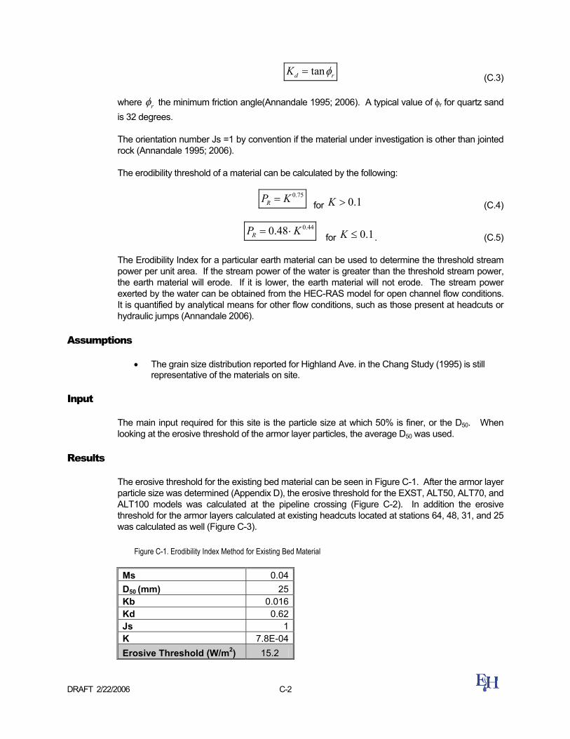
DRAFT 2/22/2006 C-2
tand rK φ=
(C.3)
where rφ the minimum friction angle(Annandale 1995; 2006). A typical value of φr for quartz sand is 32 degrees.
The orientation number Js =1 by convention if the material under investigation is other than jointed rock (Annandale 1995; 2006).
The erodibility threshold of a material can be calculated by the following:
0.75
RP K= for 0.1K > (C.4)
0.440.48RP K= ⋅
for 0.1K ≤ . (C.5)
The Erodibility Index for a particular earth material can be used to determine the threshold stream power per unit area. If the stream power of the water is greater than the threshold stream power, the earth material will erode. If it is lower, the earth material will not erode. The stream power exerted by the water can be obtained from the HEC-RAS model for open channel flow conditions. It is quantified by analytical means for other flow conditions, such as those present at headcuts or hydraulic jumps (Annandale 2006).
Assumptions
• The grain size distribution reported for Highland Ave. in the Chang Study (1995) is still representative of the materials on site.
Input
The main input required for this site is the particle size at which 50% is finer, or the D50. When looking at the erosive threshold of the armor layer particles, the average D50 was used.
Results
The erosive threshold for the existing bed material can be seen in Figure C-1. After the armor layer particle size was determined (Appendix D), the erosive threshold for the EXST, ALT50, ALT70, and ALT100 models was calculated at the pipeline crossing (Figure C-2). In addition the erosive threshold for the armor layers calculated at existing headcuts located at stations 64, 48, 31, and 25 was calculated as well (Figure C-3).
Figure C-1. Erodibility Index Method for Existing Bed Material
Ms 0.04D50 (mm) 25Kb 0.016Kd 0.62Js 1K 7.8E-04Erosive Threshold (W/m2) 15.2

DRAFT 2/22/2006 C-3
Figure C-2. Erodibility Index Method for Median Armor Layer Particle Size Calculated at the Pipeline Crossing
At Pipeline Crossing Parameter EXST ALT50 ALT70 ALT100
Ms 0.09 0.09 0.09 0.09D50 (mm) 436 224 183 156
Kb 82.8 11.3 6.1 3.8Kd 0.6 0.6 0.6 0.6Js 1 1 1 1K 4.7 0.6 0.3 0.2
Erosive Threshold (W/m2) 944 392 301 244
Figure C-3. Erodibility Index Method for Median Armor Layer Particle Size Calculated for Active Headcuts
Existing Headcut Station #'s Parameter 64 48 31 25
Ms 0.09 0.09 0.09 0.09D50 (mm) 217 328 114 129
Kb 10.2 35.2 1.5 2.2Kd 0.6 0.6 0.6 0.6Js 1 1 1 1K 0.6 2.0 0.1 0.1
Erosive Threshold (W/m2) 375 648 161 190
References
1. Annandale, G. W., (1995), Erodibility, Journal of Hydraulic Research, Journal of Hydraulic Research, Vol. 33, No. 4, pp. 471-494.

APPENDIX D – ARMOR LAYER

DRAFT 2/22/2006 D-1
Appendix D: Armor Layer
Introduction
Degradation can be controlled by formation of an armor layer or by a stable slope. The formation of an armor layer will generally occur if the channel contains more than 10 percent coarse material which cannot be transported under dominant flow conditions. The Gessler method (1970) is an additional method for calculating armor layer that is not included in Pemberton and Lara (1984). The following six methods can be used for calculating armor layer formation:
1) Meyer-Peter, Muller (bedload transport equation);
2) Competent bottom velocity;
3) Lane’s tractive force theory;
4) Shields diagram;
5) Yang incipient motion; and
6) Gessler method.
Assumptions
• The grain size distribution at Highland Ave. reported in the Chang study (1995) reflects the current bed gradation at the pipeline crossing.
• Clear water, i.e. no sediment is being transported from upstream;
• The two-year discharge of 400cfs is the dominant discharge, the flow effecting the ultimate shape and hydraulics of the channel;
• The degraded channel will have the same hydraulic conditions as the existing channel;
• The ultimate slope of the degraded channel will be equal to that of the existing channel
Input
All hydraulic input data obtained from HEC-RAS results (Table D-1andTable D-2) and all gradation input obtained from the Highland Ave. grain size distribution (Figure D- 1) (Chang 1995).

DRAFT 2/22/2006 D-2
Table D-1. Input Parameters for Armor Layer and Gessler Method Calculations for EXST, ALT50, SLT70, and ALT100
Method 1: Meyer-Peter, Muller Variable EXST ALT50 ALT70 ALT100 Comment
d1 0.64 m 0.23 m 0.19 m 0.16 m mean water depth at pipeline crossing
SE_1 0.043 m/m 0.062 m/m 0.062 m/m 0.062 m/m Energy gradient slope
nls 0.03 0.03 0.03 0.03 Manning's roughness for the channel bed
D90_1 970 mm 970 mm 970 mm 970 mm Particle size at which 90 percent of the bed material is finer
K1 0.058 0.058 0.058 0.058 constant
∆p1 0.15 0.22 0.24 0.26 Decimal percentage of original bed material larger than the armor size Dc Method 2: Competent Bottom Velocity Method
Variable EXST ALT50 ALT70 ALT100 Comment Vm 4.36 m/s 3.08 m/s 2.719 m/s 2.37 m/s mean channel velocity
∆p2 0.17 0.25 0.29 0.33 Decimal percentage of original bed material larger than the armor size Dc Method 3: Lane's Tractive Force Method
Variable EXST ALT50 ALT70 ALT100 Comment d 0.64 m 0.23 m 0.19 m 0.16 m mean water depth at pipeline crossing S 0.043 m/m 0.062 m/m 0.062 m/m 0.062 m/m Energy gradient slope
∆p3 n/a 0.3 0.34 0.35 Decimal percentage of original bed material larger than the armor size Dc
Method 4: Shields Method Variable EXST ALT50 ALT70 ALT100 Comment
Tstar 0.047 0.047 0.047 0.047 Dimensionless shear stress
∆p4 0.18 0.25 0.24 0.31 Decimal percentage of original bed material larger than the armor size Dc
Method 5: Yang Incipient Motion Method Variable EXST ALT50 ALT70 ALT100 Comment
Re 2.931 x 10³ 3.62 x 10³ 3.634 x 10³ 3.751 x 10³ Reynold's number
ν 0.929 x 10⁻⁶
m2/s 0.929 x 10⁻⁶
m2/s 0.929 x 10⁻⁶
m2/s 0.929 x 10⁻⁶
m2/s kinematic viscosity @ 25 deg. C
D50 25 mm 25 mm 25 mm 25 mm Particle size at which 50 percent of the bed material is finer
∆p5 0.22 0.18 0.18 0.16 Decimal percentage of original bed material larger than the armor size Dc

DRAFT 2/22/2006 D-3
Method 6:Gessler
Variable EXST ALT50 ALT70 ALT100 Comment D50 25 mm 25 mm 25 mm 25 mm Particle size at which 50 percent of the bed material is finer
D90 970 mm 970 mm 970 mm 970 mm Particle size at which 90 percent of the bed material is finer
Q 400 ft3/s 400 ft3/s 400 ft3/s 400 ft3/s Flow rate M 2.69 2.69 2.69 2.69 Approximate bank slope (MH:1V) at sample location S 0.049 0.039 0.039 0.039 Approximate bed slope at sample location b 17 ft 50 ft 70 ft 100 ft Approximate bottom width of the channel at sample location
γs 25970 N/m3 25970 N/m3 25970 N/m3 25970 N/m3 Specific weight of sediment
γ 9800 N/m3 9800 N/m3 9800 N/m3 9800 N/m3 Specific weight of water
ρ 1000 kg/m3 1000 kg/m3 1000 kg/m3 1000 kg/m3 Density of water
υ 1.31x10⁻⁶ m2/s 1.31x10⁻⁶ m2/s 1.31x10⁻⁶ m2/s 1.31x10⁻⁶ m2/s Kinematic viscosity of water g 9.807 m/s2 9.807 m/s2 9.807 m/s2 9.807 m/s2 Acceleration due to gravity h' 2.11 ft 0.76 ft 0.62 ft 0.51 ft Depth of flow f's 0.03 0.03 0.03 0.03 Friction factor of the bank R' 1.31 ft 0.72 ft 0.61 ft 0.5 ft Hydraulic radius R's 0.55 ft 0.36 ft 0.3 ft 0.24 ft Hydraulic radius for channel sides
R'b 1.64 ft 0.76 ft 0.62 ft 0.51 ft Hydraulic radius of channel bottom P' 22.84 ft 54.8 ft 73.95 ft 103.2 ft Wetted Perimeter P's 6.84 ft 4.8 ft 4 ft 3.2 ft Wetted Perimeter for channel sides
A' 29.9 ft2 39.64 ft2 44.87 ft2 51.35 ft2 Cross sectional area
A's 3.63 ft2 1.7 ft2 1.2 ft2 0.76 ft2 Cross sectional area for channel sides
A'b 26.27 ft2 37.92 ft2 43.7 ft2 50.59 ft2 Cross sectional area of channel bottom U' 13.38 ft/s 10.09 ft/s 8.92 ft/s 7.79 ft/s Average flow velocity
∆pA50 0.15 0.19 0.19 0.21 Decimal percentage of original bed material larger than the armor size Dc

DRAFT 2/22/2006 D-4
Table D-2. Input Parameters for Armor Layer Calculations for Active Headcuts
Method 1: Meyer-Peter, Muller Variable #64 #48 #31 #25 Comment
d1 0.567 m 0.68 m 0.366 m 0.536 m mean water depth at pipeline crossing
SE_1 0.0287 m/m 0.0404 m/m 0.0213 m/m 0.0213 m/m Energy gradient slope nls 0.03 0.03 0.03 0.03 Manning's roughness for the channel bed
D90_1 970 mm 970 mm 970 mm 970 mm Particle size at which 90 percent of the bed material is finer K1 0.058 0.058 0.058 0.058 constant
∆p1 0.2 0.15 0.28 0.24 Decimal percentage of original bed material larger than the armor size Dc Method 2: Competent Bottom Velocity Method
Variable #64 #48 #31 #25 Comment
Vm 2.914 m/s 3.27 m/s 2.34 m/s 1.95 m/s mean channel velocity
∆p2 0.26 0.24 0.31 0.36 Decimal percentage of original bed material larger than the armor size Dc
Method 3: Lane's Tractive Force Method Variable #64 #48 #31 #25 Comment
d 0.567 m 0.68 m 0.366 m 0.536 m mean water depth at pipeline crossing S 0.0287 m/m 0.0404 m/m 0.0213 m/m 0.0213 m/m Energy gradient slope
∆p3 n/a n/a 0.34 n/a Decimal percentage of original bed material larger than the armor size Dc
Method 4: Shields Method Variable #64 #48 #31 #25 Comment
Tstar 0.047 0.047 0.047 0.047 Dimensionless shear stress
∆p4 0.24 0.18 0.34 0.26 Decimal percentage of original bed material larger than the armor size Dc
Method 5: Yang Incipient Motion Method Variable #64 #48 #31 #25 Comment
Vm 2.914 m/s 3.27 m/s 2.34 m/s 1.95 m/s Particle size at which 50 percent of the bed material is finer
∆p5 0.26 0.22 0.31 0.36 Decimal percentage of original bed material larger than the armor size Dc

DRAFT 2/22/2006 D-5
0
10
20
30
40
50
60
70
80
90
100
0.001 0.01 0.1 1 10 100
Grain Size, in
Perc
ent P
assi
ng
GSD @ Highland Avenue
Figure D- 1. Highland Ave. Grain Size Distribution (Chang 1995)Calculations
Calculations
The hydraulic results for the two-year discharge for all four HEC-RAS models (EXST, ALT50, ALT70, and ALT100) were used to estimate the size of the armor layer particles, depth of degradation at the pipeline crossing, and new slope using the thalweg at Baseline St. as the control point. In addition, the armor layer, depth of degradation, and associated new slope were calculated using the hydraulic results for the 2-year discharge in the EXST model for four active head cuts at chainage: 91 ft, 2511 ft, 5486 ft, and 6568 ft with drop heights of 4 ft, 5 ft, 4 ft, and 3 ft, respectively(the Gessler Method was not used in these evaluations). By evaluating the expected armor layer formation and associated degradation at existing headcuts it is possible to estimate the slope of the channel as it reaches equilibrium.
All calculations were conducted using MathCAD. The EXST armor layer and Gessler Method MathCAD Calculations can be seen on the following pages, which serves as an example calculation. Calculations for the ALT50, ALT70, and ALT100 models and the four existing headcuts were conducted using the same MathCAD calculations. The results for all of the calculations can be seen in the Results section, Table D-1.

DRAFT 2/22/2006 D-6
City Creek Degradation Limited by Armoring
Created By: Amber Fuxan Date: January 25th, 2006
Five methods are analyzed for computing the degradation limited by armoring for the Salt Creek channel (Pemberton and Lara, 1984). Calculations have been performed using the 2yr design discharge.
Method 1: Meyer-Peter, Muller d1 0.64:= mean water depth at pipeline crossing (m)
Energy Gradient slope (m/m) SE_1 0.043:=
Manning's roughness for the channel bed n1s 0.03:=
in (mm) D90_1 970:=
K1 0.058:= Constant (metric)
Dc1d1 SE_1⋅
K1n1s
D90_1
1
6
3
2
⋅
:=
Dc1 509.602= Dc1 is in (mm)
Method 2: Competent Bottom Velocity Method Vm 4.36:= mean channel velocity (m/s)
Dc2 20.2 Vm2
⋅:=
Dc2 383.994= Dc2 is in (mm)
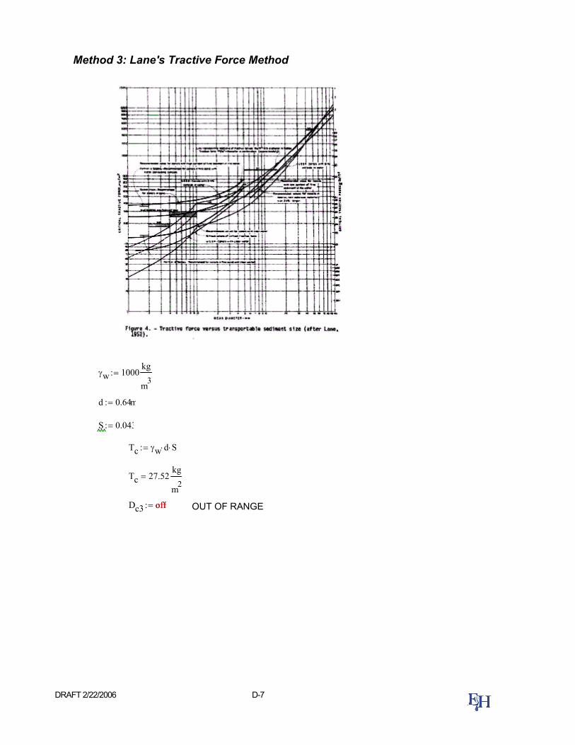
DRAFT 2/22/2006 D-7
Method 3: Lane's Tractive Force Method
γw 1000kg
m3:=
d 0.64m:=
S 0.043:=
Tc γw d⋅ S⋅:=
Tc 27.52kg
m2=
Dc3 off:= off OUT OF RANGE

DRAFT 2/22/2006 D-8
Method 4: Shields Method
γs 2650kg
m3:=
Tstar 0.047:= This value for dimensionless shear stress obtained from stable slope calculations method 3.
Dc4Tc
Tstar γs γw−( )⋅:=
Dc4 354.868mm=
Method 5: Yang Incipient Motion Method
Vm 4.36=
Dc5 0.0216Vm2
⋅ 1000⋅:=
Dc5 410.607= Answer is in mm
Dc5 mm⋅ 16.166in=
Method 6: Gessler Approach Method
From the following file: G:\Projects\City Creek\Analysis\Gessler Armor Layer\Gessler Armor Layer - City Creek.xmcd
DA50 520 mm⋅:= DA90 1300 mm⋅:=

DRAFT 2/22/2006 D-9
Summary
Dc1 509.602=
Dc2 383.994=
Dc3 :=
Dc4 354.868mm=
Dc5 410.607=
DA50 520mm=
Davg
Dc1 Dc2+Dc4mm
+DA50mm
+ Dc5+
5:=
Davg 435.814= in mm
Depth to Armor and Volume Computations
Meyer - Peter Muller Depth of Degradation
ya1 3 Dc1⋅ mm⋅:= Thickness of the armor layer, which equals two times the mean diameter of particles in the armor layer
ya1 1.529m=
Decimal percentage of original bed material larger than the armor size Dc.∆p1 0.15:=
yd1 ya11
∆p11−
⋅:=
yd1 8.663m=

DRAFT 2/22/2006 D-10
Competent Bottom Velocity Depth of Degradation
ya2 3 Dc2⋅ mm⋅:= Thickness of the armor layer, which equals two times the mean diameter of particles in the armor layer
ya2 1.152m=
Decimal percentage of original bed material larger than the armor size Dc.∆p2 0.17:=
yd2 ya21
∆p21−
⋅:=
yd2 5.624m=
Lane's Tractive Force Depth of Degradation
ya3 3 Dc3⋅ mm⋅:= Dc3 Thickness of the armor layer, which equals two times the mean diameter of particles in the armor layer
ya3 =ya3
Decimal percentage of original bed material larger than the armor size Dc. OUT OF RANGE
∆p3 :=
yd3 ya31
∆p31−
⋅:= ya3
yd3 =yd3

DRAFT 2/22/2006 D-11
Shields Diagram Depth of Degradation
ya4 3 Dc4⋅:= Thickness of the armor layer, which equals two times the mean diameter of particles in the armor layer
ya4 1.065m=
Decimal percentage of original bed material larger than the armor size Dc.∆p4 0.18:=
yd4 ya41
∆p41−
⋅:=
yd4 4.85m=
Yang Incipient Motion Depth of Degradation
ya5 3 Dc5⋅ mm⋅:= Thickness of the armor layer, which equals two times the mean diameter of particles in the armor layer
ya5 1.232m=
Decimal percentage of original bed material larger than the armor size Dc.∆p5 0.16:=
yd5 ya51
∆p51−
⋅:=
yd5 6.467m= yd5 21.217ft=
Gessler D50 Depth of Degradation
yaA50 3 DA50⋅:= Thickness of the armor layer, which equals two times the mean diameter of particles in the armor layer
yaA50 1.56 m=
Decimal percentage of original bed material larger than the armor size Dc.∆pA50 0.15:=
ydA50 yaA501
∆pA501−
⋅:=
ydA50 8.84m= D

DRAFT 2/22/2006 D-12
Gessler D90 Depth of Degradation
yaA90 3 DA90⋅:= Thickness of the armor layer, which equals two times the mean diameter of particles in the armor layer
yaA90 3.9 m=
Decimal percentage of original bed material larger than the armor size Dc.∆pA90 0.08:=
ydA90 yaA901
∆pA901−
⋅:=
ydA90 44.85m=
Average Depth of Degradation
yaAVG 2 Davg⋅ mm⋅:= Thickness of the armor layer, which equals two times the mean diameter of particles in the armor layer
yaAVG 0.872m=
Decimal percentage of original bed material larger than the armor size Dc.∆pAVG 0.17:=
ydAVG yaAVG1
∆pAVG1−
⋅:=
ydAVG 4.256m=

DRAFT 2/22/2006 D-13
City Creek Armor Layer Calculations using the Gessler Approach (Gessler 1970)
Created By: Amber Fuxan Date: January 25th, 2006
Calculations for Bed Material Location: Highland Avenue
Free-flowing Conditions: Q = 400 cfs
Particle Size Distribution
% finer d (mm)
All inputs are highlighted in yellow.
Read from Graph:
D50 25 mm⋅:=
D90 970 mm⋅:=
datas
1
5
12.5
34
52
78
92
100
0.07
.3
1.2
4.7
32
230
1000
2000
:=
finer datas0⟨ ⟩
:= size datas1⟨ ⟩
mm⋅:=
1 .10 5 1 .10 4 1 .10 3 0.01 0.1 1 100
10
20
30
40
50
60
70
80
90
100
Screen size, m
Perc
ent f
iner
finer
size
i 1 8..:=

DRAFT 2/22/2006 D-14
Input Parameters:
Q 400ft3
s⋅:= Flow rate
Q 11.327m3 s-1⋅=
M 2.69:= Approximate bank slope (MH:1V) at sample location
S 0.049mm
⋅:= Approximate bed slope at sample location
b 17ft:= Approximate bottom width of the channel at sample location
γs 25970N
m3⋅:= Specific weight of sediment
γ 9800N
m3⋅:= Specific weight of water
ρ 1000N s2
⋅
m4⋅:= Density of water
ν 0.00000131m2
s⋅:= Kinematic viscosity of water
g 9.807m s-2⋅= Acceleration due to gravity
Calculated Input Parameters:
ks D90:= Controlling roughness for the bank
ks 0.97m=
Pb b:= Pb 5.182m= Wetted perimeter of the bed
fb 2.21 2.03 log0.0251
S
⋅+
2−:=
fb 0.381= Friction factor of the bed

DRAFT 2/22/2006 D-15
Input the known value or a guess value for each of the parameters below. Subscript (s) refers to the banks of the channel, subscript (b) refers to the bed of the channel, and variables without a subscript refer to the overall parameter for the system.
h' 2.11ft:= Depth of flow
f's .03:= Friction factor of the bank
R' 1.31ft:=
R's 0.55ft:= Hydraulic radii
R'b 1.64ft:=
P' 22.84ft:= Wetted perimeters
P's 6.84ft:=
A' 29.9 ft2⋅:=
A's 3.63 ft2⋅:= Cross-sectional areas
A'b 26.27 ft2⋅:=
U' 13.38fts
⋅:= Average flow velocity (Calculations are very sensitive to this guess. If Mathcad does not calculate values below, try changing this guess.)

DRAFT 2/22/2006 D-16
The following is the system of equations that provide the relationships required to solve for the parameters listed previously. Equations based on Darcy-Weisbach's flow equation and taken from Oehy (1999)
Given
U'28 g⋅f's
R's⋅ S⋅ R'sA'sP's
U'28 g⋅fb
R'b⋅ S⋅ R'b
A'bPb
f's 2.21 2.03 logR'sks
⋅+
2−
R'A'P'
P's h' 1 M2+⋅ U'
QA'
P' Pb 2 P's⋅+
A' h' b M h'⋅+( )⋅
A' A'b 2 A's⋅+
h
fs
R
Rs
Rb
P
Ps
A
As
Ab
U
Find h' f's, R', R's, R'b, P', P's, A', A's, A'b, U',( ):=

DRAFT 2/22/2006 D-17
Solution to system of equations:
h 0.689m= Depth of flow
fs 0.365= Friction factor of the bank
R 0.531m= Overall hydraulic radius
Rs 0.518m= Hydraulic radius for the banks
Rb 0.541m= Hydraulic radius for the bed
P 9.137m= Overall wetted perimeter
Ps 1.978m= Wetted perimeter for the banks
A 4.849m2= Total cross-sectional area
As 1.024m2= The area of the bank subarea
Ab 2.802m2= The area of the bed subarea
U 2.336m s-1⋅= Average flow velocity
f8 g⋅
U2R⋅ S⋅:= f 0.374= Average friction factor

DRAFT 2/22/2006 D-18
Stress calculations:
τb γ Rb⋅ S⋅:=
τb 259.644N
m2= Bed shear stress
ubτb
ρ:=
Shear velocity, measure of the intensity of turbulent fluctuations. ub 0.51
ms
=
r 1 7..:=
davg r
sizer sizer 1−+
2:= Average grain sizes for gradation
Reynold's Number for each size fraction in gradation Rer
ub davg r⋅
ν:=
Below are equations that define of Shield's Diagram piecewise (τs1 - τs6) and τstar is an "if statement" to determine which portion of the diagram applies to a given Re value:
τs1r .115 Rer( ) .79279−⋅:=
τs2r 2.65633− 10 5−⋅ Rer( )6
⋅ 7.8492210 4−⋅ Rer( )5
⋅+ 9.2373310 3−⋅ Rer( )4
⋅−
5.4734310 2−⋅ Rer( )3
⋅ 1.6793410 1−⋅ Rer( )2
⋅− 2.3531510 1−⋅ Rer⋅+ 4.7516110 2−
⋅( )−+
...:=
τs3r .032:=
τs4r 4.8492166501818110 9−⋅ Rer( )3
⋅ 2.3693403636785910 6−⋅ Rer( )2
⋅− 3.8048049563885610 4−⋅ Rer⋅+
2.544995046687310 2−⋅+
...
:=
τs5r .046:=
τs6r .047:=
τstarr if Rer 2≤ τs1r, if Rer 8<( ) τs2r, if Rer 19≤ τs3r, if Rer 217< τs4r, if Rer 397≤ τs5r, .047,( ),( ),( ), , :=

DRAFT 2/22/2006 D-19
davgr
-41.85·10-47.5·10-32.95·10
0.018
0.131
0.615
1.5
m
= Rer
71.96291.729
31.147·1037.138·1045.096·1052.392·1055.835·10
= τstarr0.0420.046
0.047
0.047
0.047
0.047
0.047
=
τcr τstarr 1− davg r⋅ γs γ−( )⋅:= Critical shear stress for each size fraction in gradation
Ratio of critical shear stress of each size fraction to average shear stress in river ττr 1−
τcr
τb:=
Theoretical Armor Layer Calculations:
Probability that a grain of given size will not erode, fit from Gessler plot of q versus τc/τb:
qr if ττr 1− 2.8< 0.0716545194773488ττr 1−( )4⋅ 0.496929374396984ττr 1−( )3
⋅−
0.987737827575074ττr 1−( )2⋅ 0.104758490295694ττr 1−⋅−+
...
0.0527834049124749+...
, 1.0,
:=
q∆Pr qr finerr finerr 1−−( )⋅:= Intermediate Calculation
τcr0
0.514
2.194
13.946
99.559
467.39431.14·10
m-1 kg s-2⋅⋅
= davgr-41.85·10-47.5·10-32.95·10
0.018
0.131
0.615
1.5
m
= ττr 1−
0-31.979·10-38.451·10
0.054
0.383
1.8
4.391
= qr
0.0530.053
0.052
0.05
0.131
0.919
1
= q∆Pr0.2110.394
1.117
0.899
3.416
12.861
8
=

DRAFT 2/22/2006 D-20
Σq∆P
1
7
r
q∆Pr∑=
:= Σq∆P 26.898= Summation of all q∆P0 terms for use in determining ∆PA.
∆PArq∆Pr
Σq∆P:= Incremental probability function of armoring layer (missing probability = 0 for finest
grain size).
PAincompleter1
r
r
∆PAr∑=
:= Cumulative probability function of armoring layer (missing probability = 0 for finest grain size). See following page for complete grain size distribution, PAr.
r 0 7..:= Increase counter variable to account for entire set of grain sizes given initially.
PAr if r 0 0, PAincompleter,( )( ) 100⋅:= Add initial probability = 0 for finest grain size in armor layer distribution--COMPLETE ARMOR LAYER DISTRIBUTION expressed in percent.
Resulting Armor Layer Particle Size Distribution:
sizer mm⋅
-87·10-73·10-61.2·10-64.7·10-53.2·10-42.3·10-31·10-32·10
m2
= PAr
00.785
2.251
6.405
9.746
22.445
70.258
100
= ∆PAr
0-37.849·10
0.015
0.042
0.033
0.127
0.478
0.297
=

DRAFT 2/22/2006 D-21
1 .10 5 1 .10 4 1 .10 3 0.01 0.1 1 100
10
20
30
40
50
60
70
80
90
100
Armor LayerOriginal BedArmor LayerOriginal Bed
Screen size, m
Perc
ent f
iner
Read from Graph: DA50 520 mm⋅:= DA90 1300 mm⋅:=

DRAFT 2/22/2006 D-22
Results
The armor layer particle diameter and depth of degradation results for the EXST, ALT50, ALT70, and ALT100 models at the pipeline crossing can be seen in Table D-3. Table D-4 reflects the armor layer and degradation results for four existing headcuts at stations 64, 48, 31, and 25.
Table D-3. Armor Layer Results for Two-Year Discharge for All Models
Armor Layer Particle Diameter (in) Method EXST ALT50 ALT70 ALT100
Meyer-Peter, Muller 20 10 9 7 Competent Bottom Velocity 15 7.5 6 4 Lane's Tractive Force Out of range 4 4 4 Shields Diagram 14 7 6 5 Yang Incipient Motion 16 8 6 5 Gessler D50 20 16 13 12 Average Particle Diameter 17 9 7 6
Depth of Degradation (ft)
Method EXST ALT50 ALT70 ALT100 Meyer-Peter, Muller 28 9 7 5 Competent Bottom Velocity 18 6 4 2 Lane's Tractive Force - - - 2 2 2 Shields Diagram 16 5 5 3 Yang Incipient Motion 21 6 4 3 Gessler D50 29 8 6 4 Average Depth of Degradation 23 8 6 4

DRAFT 2/22/2006 D-23
Table D-4. Armor Layer Results for Two-Year Discharge for Active Headcuts
Section # 64 48 31 25 Chainage (ft) 91 2511 5486 6568 Thalweg Elevation (ft) 1488 1405 1329 1301
Method Armor Layer Particle Diameter (in) Meyer-Peter, Muller 12 20 6 8 Competent Bottom Velocity 7 9 4 3 Lane's Tractive Force Out of range Out of range Out of range Out of range Shields Diagram 8 14 4 6 Yang Incipient Motion 7 9 5 3 Average 9 13 4 5
Method Depth of Degradation (ft)
Meyer-Peter, Muller 12 28 4 7 Competent Bottom Velocity 5 7 2 1 Lane's Tractive Force - - - - - - - - - - - - Shields Diagram 7 16 2 4 Yang Incipient Motion 5 8 3 1 Average Depth of Degradation 7 15 3 3
References
Chang, Howard H. 1995. Inland Feeder Pipeline, San Bernardino Segment (Contract 3): Fluvial Study of City Creek for Pipeline Placement. Prepared for Dames and Moore.
Gessler, J. 1971. Beginning & Ceasing of Sediment Motion.” River Mechanics, H.W. Shen,
ed Hseieh Wen Shen, Fort Collins, Colorado, 7, 1-22.
Pemberton, EL and JM Lara. 1984. Computing Degradation and Local Scour. Technical Guideline for Bureau of Reclamation. Denver, Colorado.
U.S. Army Corps of Engineers (USACE). 2001. HEC-RAS River Analysis System v. 3.3.3
[computer software]. www.hec.usace.army.mil

APPENDIX E – STABLE SLOPE
APPENDIX F – BEND SCOUR
APPENDIX G – HEADCUT HYDRAULICS

DRAFT 2/22/2006 E-1
Appendix E: STABLE SLOPE
Introduction
Degradation limited by a stable slope is based on the degrading process controlled by zero or negligible transport of the material forming the bed of the stream channel. This method is applied to streams where the amount of coarse material is insufficient to form an armor layer. The methods used in Pemberton and Lara (1984) to calculate a stable slope are:
1) Schoklitsch bedload equation;
2) Meyer-Peter Muller bedload equation for beginning transport;
3) Shields diagram for no motion; and
4) Lane’s relationship for critical tractive force assuming clear water-flow in canals.
Assumptions
• The grain size distribution at Highland Ave. reported in the Chang study (1995) reflects the current bed gradation at the pipeline crossing;
• Clear water, i.e. no sediment is being transported from upstream;
• The two-year discharge of 400cfs is the dominant discharge, the flow effecting the ultimate shape and hydraulics of the channel; and

DRAFT 2/22/2006 E-2
Input
All hydraulic input data obtained from HEC-RAS results and all gradation input obtained from the Highland Ave. grain size distribution (Figure E-1).
• Table E-1. Stable Slope Input Parameters for EXST, ALT50, SLT70, and ALT100
All Methods Variable EXST ALT50 ALT70 ALT100 Comment
Q 400 cfs 400 cfs 400 cfs 400 cfs Dominant discharge QB 375.56 cfs 389.23 cfs 393.6 cfs 396.35 cfs Average flow over bed of channel B 17 ft 17 ft 17 ft 17 ft Bottom width of channel d 2.11 ft 0.76 ft 0.62 ft 0.51 ft Average flow depth R 1.31 ft 0.72 ft 0.61 ft 0.5ft Average hydraulic radius
D50 25 mm 25 mm 25 mm 25 mm Mean particle size D90 970 mm 970 mm 970 mm 970 mm Particle size at which 90% of bed material by weight is finer n 0.03 0.03 0.03 0.03 Manning's roughness coefficient for bed of the channel
Method 1: Schoklitsch Variable EXST ALT50 ALT70 ALT100 Comment
K1 0.000293 0.000293 0.000293 0.000293 Constant (metric) Method 2: Meyer-Peter, Muller
Variable EXST ALT50 ALT70 ALT100 Comment K2 0.058 0.058 0.058 0.058 Constant (metric)
Method 3: Shields Diagram Variable EXST ALT50 ALT70 ALT100 Comment
υ 0.929 x10⁻⁶
m2/s 0.929x10⁻⁶
m2/s 0.929x10⁻⁶
m2/s 0.929x10⁻⁶
m2/s Kinematic viscosity of water @ 25 degrees C
ρw 997 kg/m3 997 kg/m3 997 kg/m3 997 kg/m3 Density of water @ 25 degrees C ρs 2650 kg/m3 2650 kg/m3 2650 kg/m3 2650 kg/m3 Particle density S 0.043 m/m 0.062 m/m 0.062 m/m 0.062 m/m Energy gradient slope (first guess at stable slope)
Method 4: Lane's Tractive Force Variable EXST ALT50 ALT70 ALT100 Comment
Tc 2000 g/m2 2000 g/m2 2000 g/m2 2000 g/m2 Critical tractive force read from Lane Tractive Force diagram based on D50

DRAFT 2/22/2006 E-3
• Table E-2. Description of Control Point and Degradation Life
Grade Control Structure Location: Base Line Rd. Culvert Elevation of Thalweg of Base Line Rd. Culvert: 1296 ft Distance Between Pipeline and Base Line Rd.: 4947.18 ft Current Thalweg Elevation at Pipeline Crossing: 1430 ft Life of Degradation: 100 yr
0
10
20
30
40
50
60
70
80
90
100
0.001 0.01 0.1 1 10 100
Grain Size, in
Perc
ent P
assi
ng
GSD @ Highland Avenue
• Figure E-1. Highland Ave. Grain Size Distribution (Chang 1995) Calculations
The stable slope and depth of degradation were conducted using the two year (dominant) discharge for the EXST, ALT50, ALT70, and ALT100 HEC-RAS models. All the stable-slope equations use dominant discharge, which has been assumed as the 2-yr discharge for this site.
In order to calculate the new slope, identification of a downstream grade control or local baselevel is required. The local baselevel for City Creek is the Santa Ana River. However, for this investigation, we assumed that the culvert at Base Line Road would be maintained and that this will act as the grade control structure for the Pipeline crossing. The culvert, which is about 1 mile downstream of the crossing, will function as a grade control for the Pipeline crossing because all the flow in the creek is routed through a concrete box culvert. The depth of scour at the Pipeline crossing was calculated using this location as the grade control.

DRAFT 2/22/2006 E-4
Salt Creek Compute Long-Term Stable Slope (Grade Control @ Baseline Culvert)
Created By: Mike George Edited By: Amber Fuxan Date: January 13th, 2006
Four methods are analyzed for computing the long-term stable slope for the future design of the Salt Creek channel (Pemberton and Lara, 1984). Calculations have been performed using the 2yr design discharge.
Q 400ft3
s:= Dominant discharge for City Creek based on Log Pearson III distribution applied to
USGS gage 1105580 data
QB 375.56ft3
s:= Average flow over bed of channel (from HEC-RAS)
B 17ft:= Bottom width of channel
d 2.11ft:= Average flow depth in channel (from HEC-RAS)
R 1.31ft:= Average hydraulic radius (from HEC-RAS)
D50 25mm:= Mean particle size (based on gradations provided to E&H)
D90 970mm:= Average particle size at which 90% of bed material by weight is finer (based on gradations provided to E&H)
n 0.03:= Manning's roughness coefficient for bed of the channel
Method 1: Scholitsch Method
K1 0.000293:= Constant
SL_1 K1
D50 1000⋅
SIUnitsOf D50( )
BSIUnitsOf B( )
⋅
Q
SIUnitsOf Q( )
0.75
⋅:= D50 is in mm.
SL_1 1.822 10 3−×=
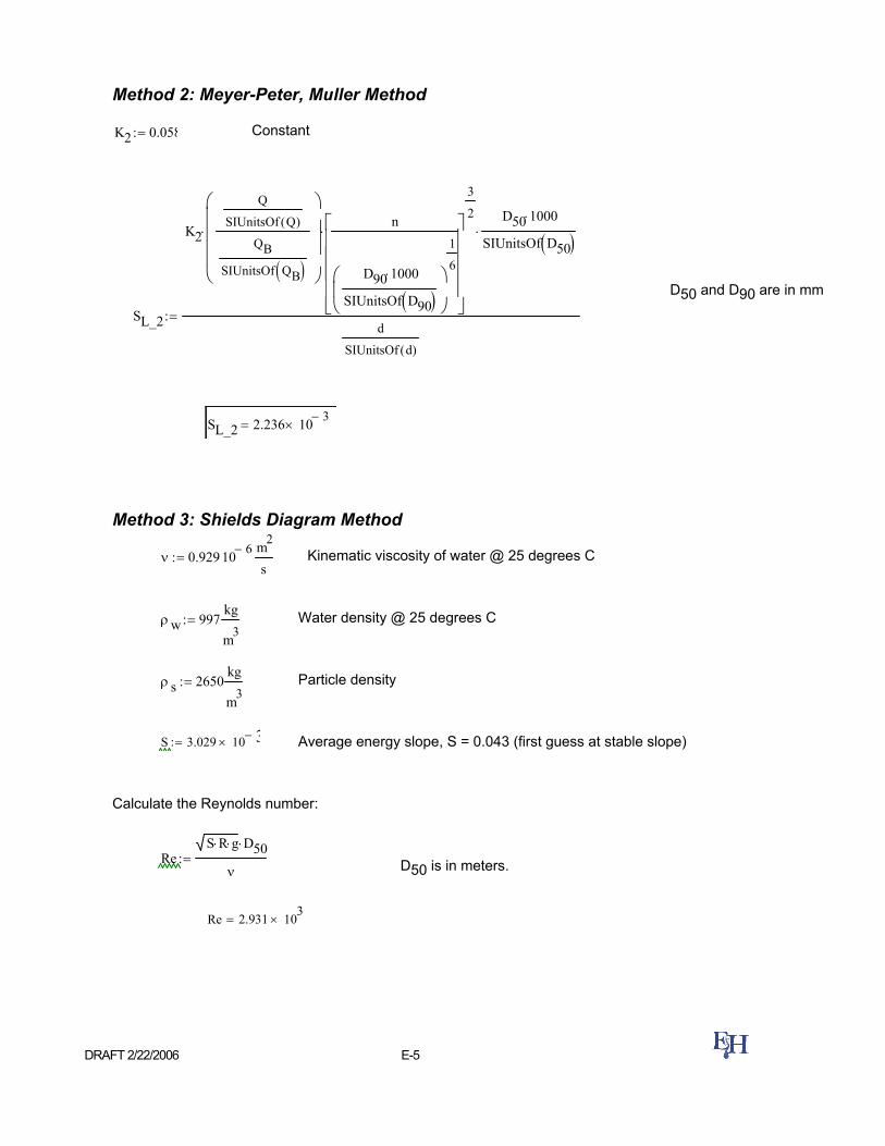
DRAFT 2/22/2006 E-5
Method 2: Meyer-Peter, Muller Method
K2 0.058:= Constant
D50 and D90 are in mm
SL_2
K2
Q
SIUnitsOf Q( )
QB
SIUnitsOf QB( )
⋅n
D90 1000⋅
SIUnitsOf D90( )
1
6
3
2⋅
D50 1000⋅
SIUnitsOf D50( )⋅
d
SIUnitsOf d( )
:=
SL_2 2.236 10 3−×=
Method 3: Shields Diagram Method
ν 0.929 10 6−⋅
m2
s:= Kinematic viscosity of water @ 25 degrees C
ρ w 997kg
m3:= Water density @ 25 degrees C
ρ s 2650kg
m3:= Particle density
S 3.029 10 3− ×:= Average energy slope, S = 0.043 (first guess at stable slope)
Calculate the Reynolds number:
ReS R⋅ g⋅ D50⋅
ν:= D50 is in meters.
Re 2.931 103× =

DRAFT 2/22/2006 E-6
Below are equations that define of Shield's Diagram piecewise (τs1 - τs6) and τstar is an "if statement" to determine which portion of the diagram applies to a given Re value:
τs1 Re( ) .115 Re .79279−⋅:=
τs2 Re( ) 2.65633− 10 5−⋅ Re6
⋅ 7.8492210 4−⋅ Re5
⋅+ 9.2373310 3−⋅ Re4
⋅−
5.4734310 2−⋅ Re3
⋅ 1.6793410 1−⋅ Re2
⋅− 2.3531510 1−⋅ Re⋅+ 4.7516110 2−
⋅( )−+
...:=
τs3 .032:=
τs4 Re( ) 4.8492166501818110 9−⋅ Re3
⋅ 2.3693403636785910 6−⋅ Re2
⋅− 3.8048049563885610 4−⋅ Re⋅+ 2.544995046687310 2−
⋅+:=
τs5 .046:=
τs6 .047:=
τstar Re( ) if Re 2≤ τs1 Re( ), if Re 8<( ) τs2 Re( ), if Re 19≤ τs3, if Re 217< τs4 Re( ), if Re 397≤ τs5, .047,( ),( ),( ), , :=
τstar Re( ) 0.047=
The stable slope may then be calculated as:
Stable slope as calculated by Shields method. SL_3 Re( )
τstar Re( ) ρ s ρ w−( )⋅ D50⋅
ρ w d⋅:=
SL_3 Re( ) 3.029 10 3−×= Iterate this value by placing it in the "S" value above
until a stable slope is reached.
Method 4: Lane's Tractive Force Method
The stable slope, SL, can be determined by making use of the following figure. Read the corresponding tractive force based on the mean particle size (D50).
D50 25mm=

DRAFT 2/22/2006 E-7
SL_4 3.119 10 3−×=
Summary of Results
SL_1 1.822 10 3−×=
SL_2 2.236 10 3−×=
SL_3 Re( ) 3.029 10 3−×=
SL_4 3.119 10 3−×=
Average 2.552 10 3−×=
Tc 2000gm
m2:= Read from graph depending on D50
SL_4Tc
ρ w d⋅:=
Average14
SL_1 SL_2+ SL_3 Re( )+ SL_4+( )⋅:=
Stable slope as calculated by Lane's tractive force method

DRAFT 2/22/2006 E-8
Results
The average slope of City Creek for current conditions is approximately 2.7*10-2, which is anticipated to change to approximately 2.6*10-3 (the average of the estimated slopes for EXST in Table E-3) for developed conditions. This is approximately a 10 fold decrease in the estimated slope.
Based on the stated assumptions, it is estimated that the rate of scour is about 1-2 ft/yr if no remedial action is taken.
• Table E-3. Estimated Stable Slope, Total Degradation, and Rate of Scour at Pipeline Crossing
Bottom Width (ft) EXST ALT50 ALT70 ALT100 Schoklitsch 0.18% 0.41% 0.53% 0.69%
Meyer-Peter, Muller 0.22% 0.60% 0.73% 0.88% Shields Diagram 0.30% 0.84% 1.00% 1.30%
Lane's Tractive Force 0.31% 0.87% 1.10% 1.30%
Stab
le S
lope
Average 0.26% 0.68% 0.84% 1.00% Schoklitsch 125 114 108 100
Meyer-Peter, Muller 123 104 98 91 Shields Diagram 119 92 85 70
Lane's Tractive Force 119 91 80 70
Deg
rada
tion
@ P
ipel
ine
(ft)
Average 121 100 93 85 Average Scour Per Year (ft/yr)* 1.21 1.00 0.93 0.85
* Assumes 100 years for full degradation depth
References
Chang, Howard H. 1995. Inland Feeder Pipeline, San Bernardino Segment (Contract 3): Fluvial Study of City Creek for Pipeline Placement. Prepared for Dames and Moore.
Pemberton, EL and JM Lara. 1984. Computing Degradation and Local Scour. Technical
Guideline for Bureau of Reclamation. Denver, Colorado. U.S. Army Corps of Engineers (USACE). 2001. HEC-RAS River Analysis System v. 3.3.3
[computer software]. www.hec.usace.army.mil

DRAFT: 2/22/06 F-1
Appendix F: Bend Scour
Introduction A channel bend exists in the vicinity of the pipeline crossing. It is necessary to investigate the additional scour that will occur due to the presence of this bend. To do so, the transverse stream power was investigated using the Chang method (1992) to evaluate the total stream power around the bend. If the magnitude of the stream power is greater than the erosive threshold of the bed material scour will occur and additional scour depth was evaluated using the Odgaard Method (1986).
The bend scour was only investigated for existing channel geometry (EXST) because the bend would most likely be removed if widening the channel was implemented.
Input All hydraulic input parameters were obtained from the EXST 2-year discharge HEC-RAS model and bed gradation characteristics were obtained from the Highland Ave. grain size distribution in the Chang study (1995).
• Table F-1. Input Parameters for the Chang Method
Chang Input Variable Value Comment Dmax 2.1 ft. Maximum depth along bend S0 0.049 ft/ft Average slope through bend rc 62.5 ft. Radius of curvature along center line ∆r 22 ft. Average width Rh 1.3 ft. Average hydraulic radius Lreach 100 ft. Length vRM51 14.3 ft/s Maximum velocity κ 0.4 von Karman's coefficient η 0.03 Manning coefficient for roughness ρ 1.94 slug/ft3 Density of water γ 62.4 pcf Unit weight of water
• Table F-2. Input Parameters for the Odgaard Method
Odgaard Input Variable Value Comment Q 400 ft3/s Dominant discharge (2-year) D 0.025 m Size of bed material S0 0.049 ft/ft Slope rc 62.5 ft. Radius of curvature along center line W 22 ft. Average water surface width dc 2.1 ft. Average flow depth υ 1.1*10-6 m2/s Kinematic viscosity ELws 1432.11 ft Water surface elevation
Calculations

DRAFT: 2/22/06 F-2
City Creek Chang Method: Transverse Stream Power Around a Bend
Created By: Amber Fuxan Date: January 25th, 2006
Parameters Dmax 2.1:= Maximum depth along bend [ft]
S0 0.049:= Average slope through the bend
rc 62.5:= Radius of curvature along center line [ft]
∆r 22:= Essentially the average width [ft]
Rh 1.3:= Average hydraulic radius [ft]
Lreach 100:= Length from [ft]
vRM51 14.3:= Should be a maximum velocity, used an average velocity because we didn't have a maximum velocity [ft/s].
U vRM51:=
κ 0.4:= von Karman's coefficient
η 0.03:= Manning coefficient for roughness
ρ 1.94:= Density of water (slug/ft^3)
γ 62.4:= Unit weight of water (pcf)
The transverse velocity, vt, can be considered a constant if known at the location of interest, i.e. at the point of maximum velocity within a particular bend. By assuming that the transverse flow velocity at the water surface in the cross section defines the magnitude of the transverse circulating velocity, the transverse velocity can be calculated with equations (8.87) and (8.88) in Chang, i.e.
fη
0.093 Rh
1
6⋅
2:=
m1 κ8f
0.5⋅:= Equation 8.31 from Chang p. 199.

DRAFT: 2/22/06 F-3
Equation 8.88 from Chang p. 215
F1f2
0.5 103
1κ
59
f2
0.5⋅−
⋅:=
F2κ
Dmax
f2
0.5⋅
m11 m1+
⋅:=
L 0 1, Lreach..:= vt0 0:=
vt L( ) vt0 3.068938401008914567210 4−⋅ L⋅ exp 4.549978259067432210210 3−
⋅ L⋅( )⋅ exp 4.5499782590674322102− 10 3−⋅ L⋅( )⋅+:=
0 20 40 60 80 1000
0.02
0.04Transverse Velocity around Bend
Distance
Velo
city
(ft/s
)
vt L( )
L
Pt L( )ρ vt L( )⋅
rc∆r⋅ U2
⋅1 m1+
m1
2
⋅1
12
m1
+
⋅ Dmax⋅:= Transverse Power along the bend
vt0
0
L
sF1Urc
⋅ e 0
L
sF2⌠⌡
d
⋅
⌠⌡
d
e 0
L
sF2⌠⌡
d−
⋅+ expand vt0 .15137125026831095056L e.32671626038048332459e-1 L⋅ e .32671626038048332459e-1−( ) L⋅⋅⋅⋅+→

DRAFT: 2/22/06 F-4
0 20 40 60 80 1000
5
10Transverse Power
Pt L( )
L
Pl γ Dmax⋅ S0⋅ vRM51⋅:= Longitudinal Power along the bend Pl 91.81973=
Pt 0( ) 0=
P L( ) Pl Pt L( )+:= Total Power
P 95( ) 100.781333= Total Power in lbf/fts. Need to multiply by .01459 to get kW/m2
0 20 40 60 80 10090
95
100
105Total Power
P L( )
L
vt s( ) vt0
0
s
sF1Urc
⋅ e 0
s
sF2⌠⌡
d
⋅
⌠⌡
d
e 0
s
sF2⌠⌡
d−
⋅+
Result P 95( ) .01459⋅:=
Result 1.47 100×=

DRAFT 2/22/2006 F-5
City Creek Odgaard Bend Scour
Created By: Dr. George Annandale Date: January 25th, 2006
MEANDER FLOW MODEL - Constant Radius Reach Solution The model in this Mathcad program is based on the paper by Odgaard, A.J., "Meander Flow Model Parts I and II", Journal of Hydraulic Engineering, Vol. 112, No. 12, December 1986, ASCE, pp. 1117-1150. The model is valid for steady, subcritical, turbulent flow in alluvial channel curves with uniform bed sediment and accounts for development and decay of flow through a bend. Constraints are: 1. The channel width is assumed to be constant. 2. The centerline radius of curvature is assumed large compared to channel width. 3. The flow-depth is small compared with the width. 4. Cross-sectional velocity components are small compared with down-channel components 5. Turbulence is isotropic

DRAFT 2/22/2006 F-6
The method has been tested with field data and was found to provide accurate representation of the long- and cross-sectional geometry of meandering rivers. The solution presented herewith is for constant radius bends. The solution for "sine-generated" meander curves is provided separately. Input requirements:
Q 400ft3
sec⋅:= D 0.0250m⋅:= S0 0.049:= rc 62.5 ft⋅:=
(two-year flood)
W 22 ft⋅:= dc 2.1 ft⋅:= ν 1 10 6−⋅
m2
sec⋅:= ELws 1432.11ft⋅:=
where Q = discharge; D = size of the bed material; S0 = slope; W = average water surface width; dc = average flow depth; ν = kinematic viscosity; rc = radius of bend at centerline. The effective water surface width, b, that is used in the calculations, is calculated as the average water surface width, W, less two times the average flow depth, dc:
b W 2 dc⋅−:=
b 17.8ft=
The average velocity at the center of the channel can therefore be calculated as:
ucQ
b dc⋅:=
uc 3.262ms
=
Assuming that the soil particle density (ρs) and the water density (ρ) is given by
ρ s 2650kg
m3⋅:=
ρ 1000kg
m3⋅:=
the particle Froude Number at the centerline of the channel can be calculated as,
FDcuc
ρ s ρ−( ) g⋅ D⋅
ρ
:=
FDc 5.128=

DRAFT 2/22/2006 F-7
Shear velocity, u*, is determined as,
ustar g S0⋅ dc⋅:=
ustar 0.555ms
=
With von Karman's coefficient, κ, equal to
κ 0.4:=
the friction factor m can be calculated as:
mdash κuc
ustar⋅:=
mdash 2.352=
and the particle Reynolds number is,
Rstar ustarDν
⋅:=
Rstar 1.386 104×=
N, a factor used in the calculation of the transverse velocity component, is equal to:
N2 mdash⋅ 1+
2 κ2
⋅ mdash⋅
:=
N 7.578=
The coefficient G that is used to calculate the variation in flow velocity along the distance s is determined as:
G2 κ
2⋅ b⋅
mdash 1+( )2 dc⋅:=
G 0.241=
With an assumed value of the Shields parameter, θ, equal to
θ 0.047:=

DRAFT 2/22/2006 F-8
and the particle shape parameter, α, equal to
α 1.27:=
it is possible to calculate the coefficients adash, bdash and cdash that are used to calculate the change in transverse bed slope in a bend as a function of curvilinear distance:
adash16 κ⋅ N⋅( ) mdash 2+( )⋅ dc⋅
3 α⋅ θ⋅ mdash 1+( )⋅ FDc⋅ b⋅:=
adash 1.754=
bdash32 κ
3⋅ N⋅( ) mdash 2+( )⋅
3 α⋅ θ⋅ mdash 1+( )2⋅ FDc⋅
:=
bdash 1.419=
cdash16 κ
2⋅ N⋅ dc⋅
mdash 1+( ) rc⋅:=
cdash 0.194=
Calculation of Variation in Bed Topography as a Function of Distance along the Bend The solution for the variation in the transverse bed slope in the stream can now be calculated by dividing the stream reach into straight and constant radius reaches, and performing the following calculations for each reach: a. Identify the starting point for each reach computation, i.e. the section with known values of STc and dSTc/ds (e.g. at the location where the cross-over between adjacent bends, where STc = 0, the derivative dSTc/ds (or, in dimensionless form, dSTc/dσ)may often be taken to be zero. Additional Input Required are the following: The transverse slope at the upstream end of the Constant Radius Reach is:
STci 0.00:=
It is also required to quantify the rate of change of the transverse slope at the upstream end of the Constant Radius Reach (dSTc/dσ) represented by STcRC0, as follows:
STcRC0 0:=

DRAFT 2/22/2006 F-9
The value of the transverse bed slope for the fully developed, constant radius bend flow can be calculated as follows,
STc0 3α
2⋅
θ( ) mdash 1+( )⋅ FDc⋅ dc⋅ b⋅
κ mdash 2+( )⋅ b⋅ rc⋅⋅:=
STc0 0.137=
The progression of STc depends on whether the system is over-, critically, or under-damped. The distinction as to whether the system is over- or critically damped, or whether it is under-damped can be made for the dimensionless distance, σ = s/b, along the bend, as follows (s= distance along centerline of channel, b = effective channel width):
For, α' 90deg:= Inscribed angle along bend
smax rc α'⋅:= s0smax
10:=
s1smax
10
2smax10
, smax..:=
σ s1( )s1b
:= σis0b
:=
The remainder of the calculations can be completed as follows:
For
ψSTcRC0
STc0 STci−:=
ψ 0=
and,
ω 0.5 4 bdash⋅ adash2
−⋅:= φ atanψ−
ω
adash2 ω⋅
+
:=
ω 0.806= φ 0.827=

DRAFT 2/22/2006 F-10
and
λ1 0.5 adash− adash2 4 bdash⋅−+
⋅:=
λ2 0.5 adash− adash2 4 bdash⋅−−
⋅:=
λ1 0.877− 0.806i+= λ2 0.877− 0.806i−=
the value of the function E (equation 34 in the Odgaard paper) that is a function of the system's damping characteristics can be calculated as follows:
E s1( ) 1ψ
ω
adash2 ω⋅
−
2
+
cos ω σ s1( ) σi−( )⋅ φ− e0.5− adash⋅ σ s1( ) σi−( )⋅
⋅
⋅ adash2 4 bdash⋅≤if
eλ1 σ s1( ) σi−( )⋅ λ2 ψ+
λ2 λ1−⋅
eλ2 σ s1( ) σi−( )⋅ λ1 ψ+
λ2 λ1−⋅
− otherwise
:=
The change in transverse slope along the bend is therefore as follows:
STc s1( ) STc0 STc0 STci−( ) E s1( )⋅−:=
Transverse Slope STc as a Function of Distance s
0 5 10 15 20 25 300
0.05
0.1
0.15
Perimeter Distance (m)
Tran
sver
se B
ed S
lope
at r
c
STc s1( )
s1

DRAFT 2/22/2006 F-11
For a curved reach, the change in depth is:
β s1( ) STc s1( )rcdc
⋅:=
and,
d r s1,( ) dcrrc
β s1( )⋅:= Er r s1,( ) ELws d r s1,( )−:=
smaxsmax
UnitsOf smax( ):=
rcrc
UnitsOf rc( ):= dcdc
UnitsOf dc( ):=
bb
UnitsOf b( ):=
N1 10:=
Freeboard 0 ft⋅:= Freeboard is difference between ELws and the ground surface
ELconcave Freeboard( ) ELws Freeboard+:= assign ground surface on concave side of bend
ELconc ELconcave Freeboard( ):=
ELconvex ELws:= assign ground surface on convex side of bend
ELwsELws
UnitsOf ELws( ):=
ELconcELconc
UnitsOf ELconc( ):= ELconvexELconvex
UnitsOf ELconvex( ):=

DRAFT 2/22/2006 F-12
d x y( )
dr k, 0←
θ r k, 0←
xr k, 0←
yr k, 0←
ELg1 ELconvex←
ELg2 ELconc←
r 1 2, N1 3⋅..∈for
k 1 2, N1 3⋅..∈for
s2 ksmaxN1
⋅←
r2 rcb2
− rbN1
⋅+←
σs2b
←
E 1ψ
ω
adash2 ω⋅
−
2
+
cos ω σ σi−( )⋅ φ− e0.5− adash⋅ σ σi−( )⋅
⋅
⋅ adash2 4 bdash⋅≤if
eλ1 σ σi−( )⋅ λ2 ψ+
λ2 λ1−⋅
eλ2 σ σi−( )⋅ λ1 ψ+
λ2 λ1−⋅
− otherwise
←
STC STc0 STc0 STci−( ) E⋅−←
β1 STCrcdc
⋅←
dr k, dcr2rc
β1
⋅←
dr k, ELws dr k,−←
θ r k,s2rc
←
xr k, r2 cos θ r k,( )⋅←
yr k, r2 sin θ r k,( )⋅←
r 1 2, N1..∈for
k 1 2, N1..∈for
k' k N1−←
s2 k'smaxN1
⋅←
r2 rcb2
− rrc
b2
−
2 N1⋅ 1+⋅−←
dr k, ELg1←
r N1 1+ N1 2+, 2 N1⋅..∈for
k N1 1+ N1 2+, 2 N1⋅..∈for
:=

DRAFT 2/22/2006 F-13
X submatrix x 1, N1, 1, N1,( ):=
Y submatrix y 1, N1, 1, N1,( ):=
D submatrix d 1, N1, 1, N1,( ):=
X2 submatrix x N1 1+, 2N1, N1 1+, 2N1,( ):=
Y2 submatrix y N1 1+, 2N1, N1 1+, 2N1,( ):=
D2 submatrix d N1 1+, 2N1, N1 1+, 2N1,( ):=
X3 submatrix x 2 N1⋅ 1+, 3N1, 2 N1⋅ 1+, 3N1,( ):=
Y3 submatrix y 2 N1⋅ 1+, 3N1, 2 N1⋅ 1+, 3N1,( ):=
D3 submatrix d 2 N1⋅ 1+, 3N1, 2 N1⋅ 1+, 3N1,( ):=
DD stack D 0⟨ ⟩D 1⟨ ⟩
, D 2⟨ ⟩, D 3⟨ ⟩
, D 4⟨ ⟩, D 5⟨ ⟩
, D 6⟨ ⟩, D 7⟨ ⟩
, D 8⟨ ⟩, D 9⟨ ⟩
,( ):=
DD2 stack D20⟨ ⟩
D21⟨ ⟩
, D22⟨ ⟩
, D23⟨ ⟩
, D24⟨ ⟩
, D25⟨ ⟩
, D26⟨ ⟩
, D27⟨ ⟩
, D28⟨ ⟩
, D29⟨ ⟩
,
:=
DD3 stack D30⟨ ⟩
D31⟨ ⟩
, D32⟨ ⟩
, D33⟨ ⟩
, D34⟨ ⟩
, D35⟨ ⟩
, D36⟨ ⟩
, D37⟨ ⟩
, D38⟨ ⟩
, D39⟨ ⟩
,
:=
XX stack X 0⟨ ⟩X 1⟨ ⟩
, X 2⟨ ⟩, X 3⟨ ⟩
, X 4⟨ ⟩, X 5⟨ ⟩
, X 6⟨ ⟩, X 7⟨ ⟩
, X 8⟨ ⟩, X 9⟨ ⟩
,( ):=
XX2 stack X20⟨ ⟩
X21⟨ ⟩
, X22⟨ ⟩
, X23⟨ ⟩
, X24⟨ ⟩
, X25⟨ ⟩
, X26⟨ ⟩
, X27⟨ ⟩
, X28⟨ ⟩
, X29⟨ ⟩
,
:=
XX3 stack X30⟨ ⟩
X31⟨ ⟩
, X32⟨ ⟩
, X33⟨ ⟩
, X34⟨ ⟩
, X35⟨ ⟩
, X36⟨ ⟩
, X37⟨ ⟩
, X38⟨ ⟩
, X39⟨ ⟩
,
:=

DRAFT 2/22/2006 F-14
YY stack Y 0⟨ ⟩Y 1⟨ ⟩
, Y 2⟨ ⟩, Y 3⟨ ⟩
, Y 4⟨ ⟩, Y 5⟨ ⟩
, Y 6⟨ ⟩, Y 7⟨ ⟩
, Y 8⟨ ⟩, Y 9⟨ ⟩
,( ):=
YY2 stack Y20⟨ ⟩
Y21⟨ ⟩
, Y22⟨ ⟩
, Y23⟨ ⟩
, Y24⟨ ⟩
, Y25⟨ ⟩
, Y26⟨ ⟩
, Y27⟨ ⟩
, Y28⟨ ⟩
, Y29⟨ ⟩
,
:=
YY3 stack Y30⟨ ⟩
Y31⟨ ⟩
, Y32⟨ ⟩
, Y33⟨ ⟩
, Y34⟨ ⟩
, Y35⟨ ⟩
, Y36⟨ ⟩
, Y37⟨ ⟩
, Y38⟨ ⟩
, Y39⟨ ⟩
,
:=
DD stack DD DD2, DD3,( ):=
XX stack XX XX2, XX3,( ):=
YY stack YY YY2, YY3,( ):=
Depth augment XX YY, DD,( ):=
max DD( ) 436.507= S0 0.049:= rc 62.5 ft⋅:=
max XX( ) 27.266=
max YY( ) 27.606= ν 1 10 6−
⋅m2
sec⋅:=
min DD( ) 435.386=
min XX( ) 0=
min YY( ) 0.122=

DRAFT 2/22/2006 F-15
Scour Depth due to Bend:
Scour max DD( ) min DD( )−dc
SIUnitsOf dc( )−:=
Scourmax Scour m⋅:=
Scourmax 1.579ft= below the original river bed
mesh 100:=
3D Image of Bed Topography around a Bend
XX YY, DD,( )

DRAFT 2/22/2006 F-16
Results
Due to the fact that the total bend stream power exceeds the erosive threshold of the existing bed materials (15.2 W/m2), scour can be expected around the bend. The expected stream power and additional scour due to the bend can be seen in Table F-3.
• Table F-3. Results for the Chang and Odgaard Methods
Chang Transverse Stream Power At end of Curve (95ft) 0.13 kW/m2
Total Stream Power At end of Curve (95ft) 1.47 kW/m2
Odgaard Depth of excess degradation at 95 ft through the bend: 1.578 ft
References
Chang, Howard H. 1992. Fluvial Processes in River Engineering. Krieger Publishing Company. Malabar, Florida.
Odgaard, A.J., "Meander Flow Model Parts I and II", Journal of Hydraulic Engineering,
Vol. 112, No. 12, December 1986, ASCE, pp. 1117-1150.

DRAFT 2/22/2006 G-1
Appendix G: Headcut Hydraulics
Introduction
Headcuts larger than 6 ft were observed during the site visit. It was deemed necessary to estimate the anticipated stream power produced by the impact of a jet falling over the head cut and the stream power of the back roller to adequately protect the pipeline from headcut migration. Superciritcal flow was observed for all discharges and for all models in HEC-RAS, therefore, a procedure developed by Chamani and Beirami (2002) for supercritical flow over headcuts was utilized.
Assumptions
• The approach slope is equal to zero. • A rectangular channel. • It is a free overfall, the nappe is unsubmerged. • The density is assumed constant throughout the calculation. The change in density
due to aeration is neglected. • Uniform velocity distribution throughout, α = 1 and β = 1. • Hydrostatic pressure distribution on the flow upstream, downstream, and at the pool. • Friction losses are negligible. • The jet angle where it hits the pool (ϕ) is equal to jet angle at the nappe base (β),
see Figure 1. • The retardation of jet velocity at the pool level affects only the vertical velocity
component, not the horizontal. Input
All hydraulic input parameters were obtained from the cross sections upstream of the headcuts in the EXST, ALT50, ALT70, and ALT100 2-year discharge HEC-RAS models.
• Table G-1. Input Parameters for the Headcut Calculations at the Pipeline Crossing
Headcut Hydraulics Variable EXST ALT50 ALT70 ALT100 Comment
q 25.2 ft2/s 7.7 ft2/s 5.6 ft2/s 3.9 ft2/s Unit discharge (discharge/avg width) H 15 ft 5 ft 4 ft 3 ft Drop height (armor layer depth of degradation)
Fr1 1.95 2.08 2.01 1.94 Approach Froude number, upstream from drop
• Table G-2. Input Parameters for Existing Headcut Calculations
Headcut Hydraulics Cross-Section Station
Variable 64 57 56 48 35 31 24
Comment
q 19.8 ft2/s 4.6 ft2/s 15 ft2/s 21.2 ft2/s 11.9 ft2/s 9.4 ft2/s 5.3 ft2/s Unit discharge (discharge/avg width)
H 4 ft 3 ft 6 ft 5 ft 4 ft 4 ft 3 ft Drop height (armor layer depth of degradation)
Fr1 1.55 2.74 1.95 1.75 1.41 1.31 1.24 Approach Froude number, upstream from drop

DRAFT 2/22/2006 G-2
Calculations
The flow characteristics for each headcut analyzed were derived from HEC-RAS results at the location of the pipeline crossing and at the location of existing headcuts. The inputs for the stream power calculation are unit discharge, drop height, and approach Froude number. The unit discharge was found by dividing the discharge by the average width. The drop height used for the EXST, ALT50, ALT70, and ALT100 headcut calculations correlates to the expected average degradation due to armoring at the pipeline crossing. The drop heights for the existing headcuts are the current drop heights of the headcuts on site as seen in the topographic AutoCAD drawing. See attached MathCAD sheet for an example of the calculations.

DRAFT 2/22/2006 G-3
City Creek Supercritical flow Over Headcuts
Created By: Amber Fuxan Date: January 25th, 2006
This sheet calculates the stream power in the backroller of a jet plunging over a headcut, with a supercritical approach flow. It also assumes that the downstream depth, Y2, is unknown.
Given: Unit discharge, drop height, approach Froude number.
γ 9820N
m3⋅:=
q 18ft2
s⋅:= Unit discharge
g 9.807m
s2=
H 15 ft⋅:= Drop height
Fr1 1.95:= Approach Froude Number, upstream from the drop.
The upstream cross-section has the subscript 1. The downstream cross-section has the subscript 2. The pool characteristics have the subscript, P.
From given parameters calculate the critical depth, approach depth, and velocity. (Assuming a prismatic rectangular channel.)
ycq2
g
1
3
:= yc 0.658m= Critical Depth (yc)
Y1q2
g Fr12
⋅
1
3
:= Y1 1.384ft= Approach Depth (Y1)

DRAFT 2/22/2006 G-4
V1qY1
:= V1 13.01fts
= Approach Velocity (V1)
Yp1 1.018m:= Estimated value, used in iteration.
A2 Fr1
2⋅
1 2Fr12
+:= A 0.884=
A and B are defined and used by Chamani and Beirami(2002).
B 1 0.5 Fr12
⋅+HY1
+Yp1Y1
−:= B 3.366=
β is the angle at which the jet strikes the downstream channel bed. β acos
1− 18A
2 B⋅++
2
:= β 1.278=
Gill (1979) used the momentum equation to show the reduction in flow velocity as the jet struck the pool. Vm = 0.5V(1-cos(β)). Where V is the jet velocity above the pool. This equation combined with the energy equation is used by Chamani and Beirami (2002) to find the relationship between V and the pool depth, Yp.
Vm121 cos β( )+( )⋅ 2 g⋅ Y1 1 0.5 Fr1
2⋅+
⋅ H+ Yp1−
⋅⋅:=
The mean velocity of jet in mixing zone just below pool surface, Vm. Vm 6.235
ms
=

DRAFT 2/22/2006 G-5
The downstream flow depth, Y2, can be found using Gill's method and the energy equation:
Y2 .02 m⋅:= Guess value, used for solve block below.
f Y2( ) Y23 1
2 g⋅Vm2 2 g⋅ Yp1⋅+
⋅ Y2
2⋅
−q2
2g+:=
Given
f Y2( ) 0
Y2 Find Y2( ):=
Y2 0.227m= Downstream flow depth (Y2).
Note: 0<Y2<yc yc 0.658m= yc 2.159ft=
The pool depth, YP,can be calculated using the momentum and continuity principles for a control volume between cross-sections 1 and 2.
Yp Y1Y2Y1
2
2 Fr12
⋅Y1Y2
⋅+ 2 Fr1
2⋅ 1+
−⋅:=
Yp 1.018m= Iterate by changing Yp1 until error is minimized.
errorYp Yp1−
Yp100⋅:= error 8.091 10 3−
×= Minimize Error
Calculate change in energy between upstream and downstream of the drop.
∆E H
qY1
2
2g+ Y1+ Y2−
qY2
2
2g−:=
∆E 2.795m=
Find the rate of energy dissipation at the downstream end of the jet (Erodibility eq. 2)
Ptotal γ q⋅ ∆E⋅:=
Rate of energy dissipation at the downstream end of the jet. Ptotal 45.903
kWm
=

DRAFT 2/22/2006 G-6
Find the rate of energy dissipation in the backroller (Erodibility eq. 9).
q3q 1 cos β( )−( )⋅
1 cos β( )+:=
q3 0.924m2
s= Unit discharge for the backroller.
Pbackroller γ q3⋅Vm2
2g⋅:=
Rate of energy dissipation in the backroller. Pbackroller 17.984
kWm
=
Find the rate of energy dissipation for the jet impacting the pool/bed.
Pimpact Ptotal Pbackroller−:=
Rate of energy dissipation at jet impact. Pimpact 27.92
kWm
=
To find the stream power per unit width, you need to divide by a length. For the back roller the length is (the depth of the pool plus the distance from the drop to jet impact). The location of the jet impact is needed.
θ 0:= Take off angle from drop.
Vm 6.235ms
= Impact velocity, calculated above.
Dimensions of inner core of Jet (Ski-Jump Jet Hydraulics MathCAD worksheet). Dj Y1
V1Vm
⋅:=
Turbulence coefficient (Ski-Jump Jet Hydraulics MathCAD worksheet). K2 1:=
hvV12
2g:=
hv 0.802m=

DRAFT 2/22/2006 G-7
Lt tan θ( ) tan θ( )2 1−( ) H⋅
K2 Y1 hv+( )⋅ cos θ( )2⋅
−+
2⋅ K2⋅ Y1 hv+( )⋅ cos θ( )⋅:=
Location where jet impacts the plunge pool, equation from Ski-Jump Hydraulics MathCAD worksheet.
Lt 4.73m=
Lbackroller Yp Lt+( ):= Length the backroller is in contact with.
Lbackroller 5.748m=
With area and backroller stream power calculated, the stream power per unit width for the backroller can be calculated.
Rate of energy dissipation per unit area in the backroller.
PbackrollerLbackroller
3.12854kW
m2=
To find the stream power per unit width, you need to divide by an area. For the jet impact, the area is (unit width) times (dimensions of the inner core of the jet).
Limpact Dj:=
Limpact 0.336m=
With area and impact stream power calculated, the stream power per unit width for the jet impact can be calculated.
PimpactLimpact
83.019kW
m2= Rate of energy dissipation per unit area at jet
impact.
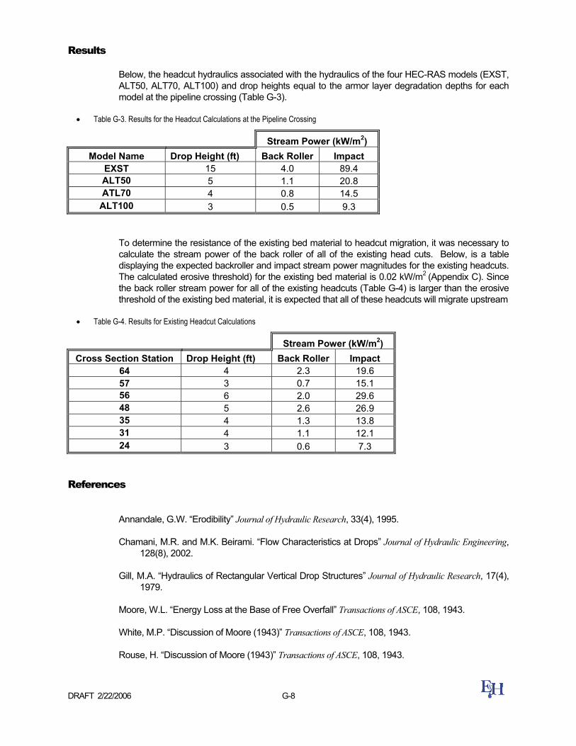
DRAFT 2/22/2006 G-8
Results
Below, the headcut hydraulics associated with the hydraulics of the four HEC-RAS models (EXST, ALT50, ALT70, ALT100) and drop heights equal to the armor layer degradation depths for each model at the pipeline crossing (Table G-3).
• Table G-3. Results for the Headcut Calculations at the Pipeline Crossing
Stream Power (kW/m2) Model Name Drop Height (ft) Back Roller Impact
EXST 15 4.0 89.4 ALT50 5 1.1 20.8 ATL70 4 0.8 14.5
ALT100 3 0.5 9.3
To determine the resistance of the existing bed material to headcut migration, it was necessary to calculate the stream power of the back roller of all of the existing head cuts. Below, is a table displaying the expected backroller and impact stream power magnitudes for the existing headcuts. The calculated erosive threshold) for the existing bed material is 0.02 kW/m2 (Appendix C). Since the back roller stream power for all of the existing headcuts (Table G-4) is larger than the erosive threshold of the existing bed material, it is expected that all of these headcuts will migrate upstream
• Table G-4. Results for Existing Headcut Calculations
Stream Power (kW/m2) Cross Section Station Drop Height (ft) Back Roller Impact
64 4 2.3 19.6 57 3 0.7 15.1 56 6 2.0 29.6 48 5 2.6 26.9 35 4 1.3 13.8 31 4 1.1 12.1 24 3 0.6 7.3
References
Annandale, G.W. “Erodibility” Journal of Hydraulic Research, 33(4), 1995.
Chamani, M.R. and M.K. Beirami. “Flow Characteristics at Drops” Journal of Hydraulic Engineering, 128(8), 2002.
Gill, M.A. “Hydraulics of Rectangular Vertical Drop Structures” Journal of Hydraulic Research, 17(4), 1979.
Moore, W.L. “Energy Loss at the Base of Free Overfall” Transactions of ASCE, 108, 1943.
White, M.P. “Discussion of Moore (1943)” Transactions of ASCE, 108, 1943.
Rouse, H. “Discussion of Moore (1943)” Transactions of ASCE, 108, 1943.

APPENDIX F-2 WEST Foothill Pipeline Scour Analysis Draft


DRAFT REPORT
SCOUR EVALUATION FOR THE FOOTHILL PIPELINE CROSSING CITY CREEK IN THE CITY OF HIGHLAND, CA
December 22, 2008
Prepared For:
SAN BERNARDINO VALLEY MUNICIPAL WATER DISTRICT 380 East Vanderbilt Way SAN BERNARDINO, CA 92408 (909)-387-9200
Prepared By: WEST CONSULTANTS, INC. 11440 W. BERNARDO COURT, SUITE 360 SAN DIEGO, CA 92127-1644 (858) 487-9378
WEST Project No.990C01

WEST Consultants, Inc. Foothill Pipeline Scour Analysis
i
TABLE OF CONTENTS
1. Introduction.......................................................................................................................... 1-1 1.1. Purpose......................................................................................................................... 1-1 1.2. Reach Description........................................................................................................ 1-2 1.3. Data Collection ............................................................................................................ 1-3 1.4. Acknowledgments........................................................................................................ 1-4
2. Hydrology ............................................................................................................................ 2-1 2.1. Flood Frequency Discharge Data................................................................................. 2-1 2.2. Historical Hydrograph ................................................................................................. 2-1 2.3. 100-Year Hydrograph .................................................................................................. 2-4
3. Hydraulic Analysis............................................................................................................... 3-1 3.1. Model Development..................................................................................................... 3-1 3.2. Model Parameters ........................................................................................................ 3-1 3.3. Bridges and Culverts.................................................................................................... 3-1
4. Sediment Transport Analysis............................................................................................... 4-1 4.1. General......................................................................................................................... 4-1 4.2. Sediment Parameters.................................................................................................... 4-2 4.3. Bed Sediment Characteristics ...................................................................................... 4-2 4.4. Sediment Boundary Conditions ................................................................................... 4-6 4.5. Quasi-Unsteady Flow Data .......................................................................................... 4-7 4.6. Results.......................................................................................................................... 4-8 4.7. Local Scour ................................................................................................................ 4-10 4.8. Total Scour................................................................................................................. 4-11
5. References............................................................................................................................ 5-1
LIST OF TABLES
Table 2-1. Adopted Flood Frequency Results for City Creek. .................................................... 2-1
Table 2-2. 89-year Historic Hydrograph (Mean Daily Flows). ................................................... 2-2
Table 2-3. 25-year Precipitation Values. ..................................................................................... 2-4
Table 4-1. Equilibrium Sediment Inflow Load............................................................................ 4-6
Table 4-2. Estimated Antidune Scour. ....................................................................................... 4-11
Table 4-3. Total Predicted Scour at Pipeline Crossing. ............................................................. 4-11

WEST Consultants, Inc. Foothill Pipeline Scour Analysis
ii
LIST OF FIGURES
Figure 1-1. Location Map. ........................................................................................................... 1-2
Figure 1-2. FEMA FIRM Panel No. 06071C8702H.................................................................... 1-3
Figure 2-1. USGS Gage No. 11055800 Record........................................................................... 2-2
Figure 2-2. Calculated 100-year Storm Hydrograph for City Creek. .......................................... 2-4
Figure 3-1. City Creek HEC-RAS Cross Sections. ..................................................................... 3-1
Figure 4-1. Sediment Sample Locations...................................................................................... 4-3
Figure 4-2. Sediment Gradation Data (1). ................................................................................... 4-4
Figure 4-3. Sediment Gradation Data (2). ................................................................................... 4-5
Figure 4-4. Sediment Inflow Load Rating Curve. ....................................................................... 4-7
Figure 4-5. Long-Term Invert Change at Pipeline Crossing - No Sediment Load...................... 4-8
Figure 4-6. Long-Term Invert Change at Pipeline Crossing – 20% of Equilibrium Sediment Load (Laursen Method Failed to Provide Stable Solution)……………. ............. 4-9
Figure 4-7. 100-Year Flood Invert Change at Pipeline Crossing - No Sediment Load............. 4-10
LIST OF APPENDICES
Appendix A: HEC-RAS Hydraulic Model Results

INTRODUCTION
WEST Consultants, Inc. Foothill Pipeline Scour Analysis
1-1
1. Introduction
1.1. Purpose The purpose of this study is to perform a sediment transport, scour, and channel stability analysis for the City Creek Channel (Channel) near the San Bernardino Valley Municipal Water District (District) Foothill Pipeline. The pipeline is located about 1,000 ft downstream of Highland Avenue in the City of Highland, California. The results of this study will be utilized in the selection and design of the pipeline scour protection alternatives. The pipeline crosses under the Channel along the base of the San Bernardino Mountains. At the Channel crossing, the pipeline is encased in reinforced concrete that is 2 feet thick on the top and 1 foot thick on the sides and bottom. When constructed, the pipeline had a minimum of 8 feet of cover within the Channel. During the winter of 2004/2005, the San Bernardino County Flood Control District (SBCFCD) changed the Channel’s configuration from a wide, “braided” stream to a “single thread” earthen trapezoidal channel. This has changed the hydraulic characteristics of the channel. In April of 2006, the District visited the site and found that all of the cover had been removed from the pipeline and approximately 6 feet of the downstream side of the concrete encasement was exposed. Under emergency permits with the SBCFCD, the U.S. Army Corps of Engineers and the California Department of Fish and Game, the District arranged for the placement of large boulders on the downstream side of the pipeline to help prevent further erosion. Many of these rocks were later washed downstream which required the subsequent placement of larger rocks. The Metropolitan Water District of Southern California (MWDSC) Inland Feeder Pipeline (Inland Feeder) also crosses the Channel just upstream from the Foothill pipeline. MWDSC was aware of this problem and had already completed a scour analysis. The MWDSC scour analysis concluded that “the channel has not yet achieved equilibrium” and will continue to erode. It also concluded that there was not yet enough field work to determine the extent of erosion. MWDSC and the District shared the cost to prepare a conceptual design report. However, this report also concluded that it is difficult to recommend an alternative not knowing the final extent of scour. Given the importance of the Foothill pipeline as the foundation of regional water infrastructure in this area (it provides direct deliveries of water to four of the District’s largest customers), the goal of this study is to:
1) Estimate the long-term (50 years or longer) configuration of the City Creek channel between Highland Avenue and Base Line Road.
2) Estimate the depth and width of potential erosion that will occur at the pipeline.
3) Prepare conceptual designs and cost estimates for one or more alternatives that would protect the pipeline.
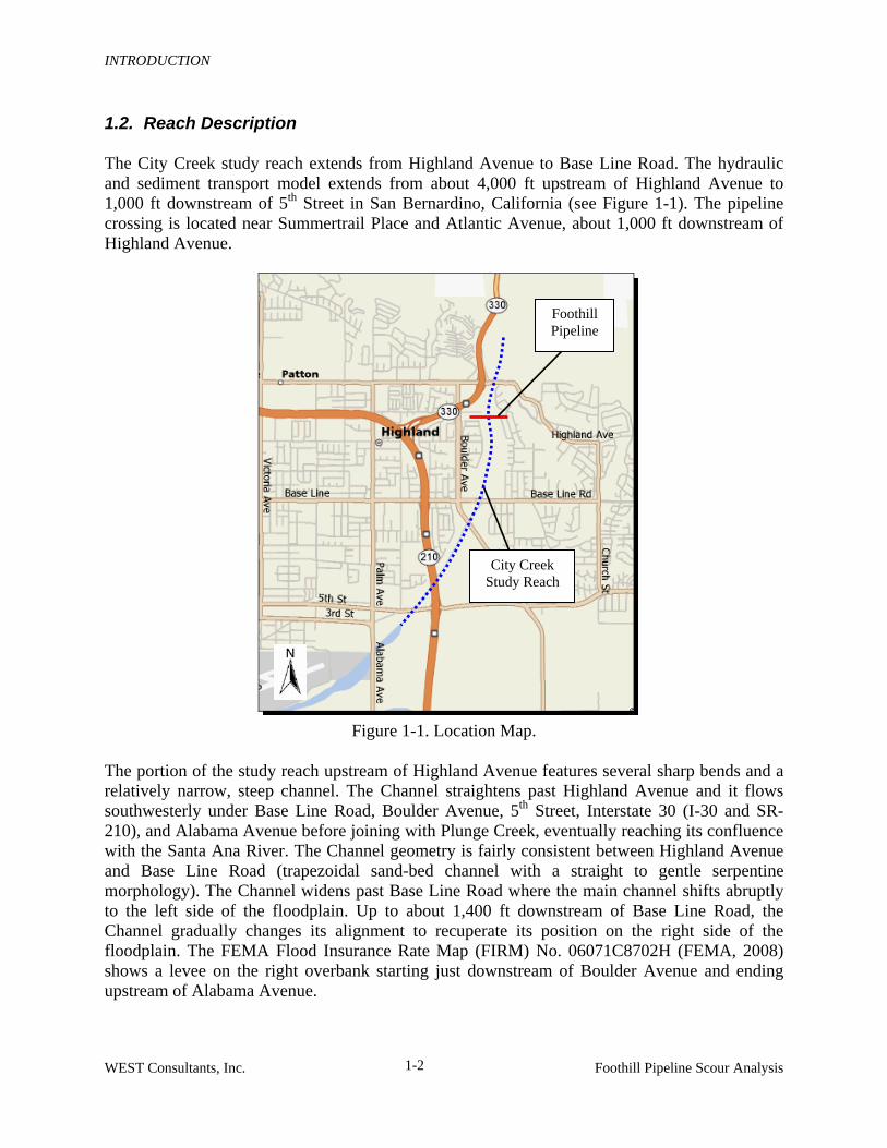
INTRODUCTION
WEST Consultants, Inc. Foothill Pipeline Scour Analysis
1-2
1.2. Reach Description The City Creek study reach extends from Highland Avenue to Base Line Road. The hydraulic and sediment transport model extends from about 4,000 ft upstream of Highland Avenue to 1,000 ft downstream of 5th Street in San Bernardino, California (see Figure 1-1). The pipeline crossing is located near Summertrail Place and Atlantic Avenue, about 1,000 ft downstream of Highland Avenue.
Figure 1-1. Location Map.
The portion of the study reach upstream of Highland Avenue features several sharp bends and a relatively narrow, steep channel. The Channel straightens past Highland Avenue and it flows southwesterly under Base Line Road, Boulder Avenue, 5th Street, Interstate 30 (I-30 and SR-210), and Alabama Avenue before joining with Plunge Creek, eventually reaching its confluence with the Santa Ana River. The Channel geometry is fairly consistent between Highland Avenue and Base Line Road (trapezoidal sand-bed channel with a straight to gentle serpentine morphology). The Channel widens past Base Line Road where the main channel shifts abruptly to the left side of the floodplain. Up to about 1,400 ft downstream of Base Line Road, the Channel gradually changes its alignment to recuperate its position on the right side of the floodplain. The FEMA Flood Insurance Rate Map (FIRM) No. 06071C8702H (FEMA, 2008) shows a levee on the right overbank starting just downstream of Boulder Avenue and ending upstream of Alabama Avenue.
City Creek Study Reach
Foothill Pipeline
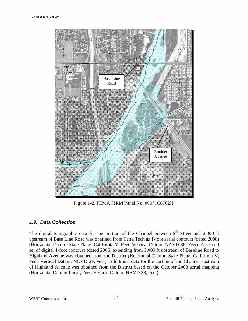
INTRODUCTION
WEST Consultants, Inc. Foothill Pipeline Scour Analysis
1-3
Figure 1-2. FEMA FIRM Panel No. 06071C8702H.
1.3. Data Collection The digital topographic data for the portion of the Channel between 5th Street and 2,000 ft upstream of Base Line Road was obtained from Tetra Tech as 1-foot aerial contours (dated 2008) (Horizontal Datum: State Plane, California V, Feet. Vertical Datum: NAVD 88, Feet). A second set of digital 1-foot contours (dated 2006) extending from 2,000 ft upstream of Baseline Road to Highland Avenue was obtained from the District (Horizontal Datum: State Plane, California V, Feet. Vertical Datum: NGVD 29, Feet). Additional data for the portion of the Channel upstream of Highland Avenue was obtained from the District based on the October 2008 aerial mapping (Horizontal Datum: Local, Feet. Vertical Datum: NAVD 88, Feet).
Base Line Road
Boulder Avenue

INTRODUCTION
WEST Consultants, Inc. Foothill Pipeline Scour Analysis
1-4
The flow frequency information for City Creek was found in the 2008 City Creek Levee report (Tetra Tech, 2008). Historical flows were downloaded from the Internet for the USGS Stream Gage No. 11055800 (City Creek, http://waterdata.usgs.gov/nwis/uv?11055800). No flow information for City Creek is indicated in the Flood Insurance Study (FIS) for San Bernardino County. The aerial images for the study reach were downloaded from the National Map Seamless Server (http://seamless.usgs.gov/). WEST performed a field reconnaissance of the site on July 17, 2008 to document field conditions necessary for the development of the sediment transport model. The field inspection included an assessment of stream behavior and morphology in the vicinity of the pipeline crossing, existing and potential scour problems, and estimates of hydraulic parameters. Observations made regarding channel stability, aggradation/degradation, hydraulic roughness, bed material size, and hydraulic or sediment transport controls were used throughout this study. WEST also collected bed sediment samples to determine streambed characteristics (representative sediment grain sizes). NMG Geotechnical Inc. analyzed the sediment samples and developed gradation curves (discussed in Section 4.3 of this report) used in the sediment transport model.
1.4. Acknowledgments Mr. Martin Teal, PE, PH, was the WEST project manager. Dr. Dragoslav Stefanovic, PE, was the lead hydraulic engineer who performed hydraulic, sediment transport, and scour analyses. Ms. Daniela Todesco, PE, assisted with the data collection and hydraulic analysis. The project manager for the District was Mr. Michael Esquer.

HYDROLOGY
WEST Consultants, Inc. Foothill Pipeline Scour Analysis
2-1
2. Hydrology The flood frequency discharge data for the Channel were obtained from Tetra Tech (2008). The historic hydrograph (for the long-term sediment transport analysis) was based on the 89-year flow record at USGS Gage No. 11055800 (one mile upstream of the pipeline crossing). The 100-year event hydrograph was generated by WEST to match the 100-year peak flow obtained from the flood frequency analysis.
2.1. Flood Frequency Discharge Data The flood frequency discharges for the City Creek were estimated by Tetra Tech (2008) as follows:
Table 2-1. Adopted Flood Frequency Results for City Creek.
COMPUTED PROBABILITY CURVE FLOW (CFS) PERCENT
CHANCE EXCEEDANCE
RETURN FREQUENCY
(YEAR) At USGS
Stream Gauge 11055800
At Boulder Avenue At 5th Street
0.2 500 21,000 21,780 28,220 0.5 200 14,000 14,520 18,820 1.0 100 10,100 10,470 13,570 2.0 50 7,100 7,360 9,540 5.0 20 4,060 4,210 5,460
10.0 10 2,500 2,590 3,360 20.0 5 1,390 1,440 1,870
2.2. Historical Hydrograph
A continuous historical hydrograph for City Creek consisting of 89 years of mean daily flows was developed by WEST based on the records of USGS Gage No. 11055800 – City Creek at Highland Avenue (see Figure 2-1). Only days in which the gage had positive readings were considered. This historical hydrograph was prepared to simulate the long-term bed changes in the study reach as requested by the District.
The final hydrograph used in this study (see Table 2-2) was reduced to 424 days by eliminating those days in which the readings (or estimates) were less than 100 cfs (flows below 100 cfs were considered to have little influence on shaping the channel morphology).

HYDROLOGY
WEST Consultants, Inc. Foothill Pipeline Scour Analysis
2-2
USGS Gage No. 11055800
0
200
400
600
800
1000
1200
1400
1600
1800
2000
2200
2400
2600
2800
3000
3200
3400
6/4/1916 2/11/1930 10/21/1943 6/29/1957 3/8/1971 11/14/1984 7/24/1998 4/1/2012
Date
Flo
w (
cfs
)
Figure 2-1. USGS Gage No. 11055800 Record.
Table 2-2. 89-year Historic Hydrograph (Mean Daily Flows).
Day 1 2 3 4 5 6 7 8 9 10 11 12 13 Q (cfs) 134 166 120 190 117 138 138 393 109 339 249 101 112
Day 14 15 16 17 18 19 20 21 22 23 24 25 26 Q (cfs) 247 149 101 520 227 137 104 216 385 288 191 143 119
Day 27 28 29 30 31 32 33 34 35 36 37 38 39 Q (cfs) 105 268 140 106 620 1040 725 840 330 157 258 628 1200
Day 40 41 42 43 44 45 46 47 48 49 50 51 52 Q (cfs) 365 191 116 134 104 129 135 310 172 131 245 142 129
Day 53 54 55 56 57 58 59 60 61 62 63 64 65 Q (cfs) 106 162 346 363 153 372 240 160 116 120 217 130 149
Day 66 67 68 69 70 71 72 73 74 75 76 77 78 Q (cfs) 115 170 254 1990 735 262 208 160 144 337 491 334 238
Day 79 80 81 82 83 84 85 86 87 88 89 90 91 Q (cfs) 192 153 123 105 140 104 136 525 507 200 110 176 203
Day 92 93 94 95 96 97 98 99 100 101 102 103 104 Q (cfs) 130 239 197 140 107 122 107 118 131 105 263 716 124
Day 105 106 107 108 109 110 111 112 113 114 115 116 117 Q (cfs) 119 294 234 122 422 547 250 150 105 318 124 131 157
Day 118 119 120 121 122 123 124 125 126 127 128 129 130 Q (cfs) 397 137 147 182 329 133 136 127 118 332 126 472 127
Day 131 132 133 134 135 136 137 138 139 140 141 142 143 Q (cfs) 134 113 140 126 119 238 153 199 150 101 221 352 192
Day 144 145 146 147 148 149 150 151 152 153 154 155 156

HYDROLOGY
WEST Consultants, Inc. Foothill Pipeline Scour Analysis
2-3
Q (cfs) 120 133 110 124 168 243 434 207 245 114 205 310 242 Day 157 158 159 160 161 162 163 164 165 166 167 168 169
Q (cfs) 541 328 202 170 190 158 127 115 104 125 322 409 144 Day 170 171 172 173 174 175 176 177 178 179 180 181 182
Q (cfs) 137 276 210 158 192 197 507 1290 320 142 120 140 120 Day 183 184 185 186 187 188 189 190 191 192 193 194 195
Q (cfs) 308 302 269 2070 1460 642 268 162 120 160 190 1020 3360 Day 196 197 198 199 200 201 202 203 204 205 206 207 208
Q (cfs) 2900 2220 1340 886 620 445 330 248 238 217 197 182 189 Day 209 210 211 212 213 214 215 216 217 218 219 220 221
Q (cfs) 166 155 148 138 136 134 134 132 123 104 118 105 104 Day 222 223 224 225 226 227 228 229 230 231 232 233 234
Q (cfs) 247 199 248 129 102 197 117 747 791 257 162 232 110 Day 235 236 237 238 239 240 241 242 243 244 245 246 247
Q (cfs) 122 411 725 408 829 740 317 226 170 138 114 126 116 Day 248 249 250 251 252 253 254 255 256 257 258 259 260
Q (cfs) 118 107 130 144 167 122 104 120 1320 291 226 331 760 Day 261 262 263 264 265 266 267 268 269 270 271 272 273
Q (cfs) 1170 741 615 645 746 474 370 280 213 170 139 120 256 Day 274 275 276 277 278 279 280 281 282 283 284 285 286
Q (cfs) 474 501 478 317 271 420 363 277 235 210 177 153 135 Day 287 288 289 290 291 292 293 294 295 296 297 298 299
Q (cfs) 118 110 104 105 176 112 115 222 124 264 145 243 269 Day 300 301 302 303 304 305 306 307 308 309 310 311 312
Q (cfs) 235 153 124 107 103 106 114 105 128 250 124 117 209 Day 313 314 315 316 317 318 319 320 321 322 323 324 325
Q (cfs) 124 152 120 109 775 364 131 168 284 260 737 783 621 Day 326 327 328 329 330 331 332 333 334 335 336 337 338
Q (cfs) 331 213 163 134 120 115 105 310 199 138 112 127 464 Day 339 340 341 342 343 344 345 346 347 348 349 350 351
Q (cfs) 728 301 215 231 224 185 169 168 150 135 125 117 110 Day 352 353 354 355 356 357 358 359 360 361 362 363 364
Q (cfs) 103 110 117 129 284 277 116 181 108 719 552 187 124 Day 365 366 367 368 369 370 371 372 373 374 375 376 377
Q (cfs) 449 264 168 132 112 103 109 102 208 222 144 135 634 Day 378 379 380 381 382 383 384 385 386 387 388 389 390
Q (cfs) 239 122 136 355 158 441 457 177 111 220 121 141 552 Day 391 392 393 394 395 396 397 398 399 400 401 402 403
Q (cfs) 110 250 195 492 1650 2000 1600 460 300 200 160 135 115 Day 404 405 406 407 408 409 410 411 412 413 414 415 416
Q (cfs) 200 150 105 182 160 500 275 400 200 150 128 120 112 Day 417 418 419 420 421 422 423 424
Q (cfs) 105 151 152 281 140 222 117 170
Table 2-2 (continued).

HYDROLOGY
WEST Consultants, Inc. Foothill Pipeline Scour Analysis
2-4
2.3. 100-Year Hydrograph
The 100-year storm hydrograph was developed by WEST following the San Bernardino County Hydrology Manual (Manual, 1986) procedures for the Unit Hydrograph Method. Because the 100-year peak flow of 10,470 cfs (at Boulder Avenue) was already estimated, WEST calibrated the Unit Hydrograph parameters to match the above peak flow. The contributing subbasin area for Gage No. 11055800 was estimated at 20.7 square miles. Point precipitation values were obtained from an online version of NOAA Atlas 14 (http://hdsc.nws.noaa.gov) as presented in Table 2-3. WEST utilized the 25-year precipitation which SBCFCD has found to match the FEMA’s 50-percent confidence level for calculating the 100-year peak flow.
Table 2-3. 25-year Precipitation Values.
25-year Precipitation (inches)
5-minutes 15-minutes 1 hour 2 hours 3 hours 6 hours 0.48 0.91 1.52 2.15 2.70 4.12
The lag was estimated at 1.2 hours based on the stream length, centroidal stream length, and drainage slope using the empirical formula presented in the Manual and it was adjusted to 1.1125 hours to match the 100-year peak flow value of 10,470 cfs. The maximum loss rate was calculated as 0.33 in/hr based on studies from nearby basins (e.g., WEST 2009 – Daley Basin). Initial abstractions were omitted for conservative purposes. The S-graph for Mountain Conditions was used based on the Manual guidelines. A hydrologic model for the City Creek basin was created using HEC-HMS Version 3.3. The resulting 100-year hydrograph utilized in this study is shown in Figure 2-2.
City Creek 100-yr Hydrograph at Boulder Avenue
0
2000
4000
6000
8000
10000
12000
0:00 2:00 4:00 6:00 8:00 10:00 12:00 14:00 16:00 18:00
Time (hours)
Flo
w (
cfs
)
City Creek 100-yr Hydrograph at Boulder Avenue
0
2000
4000
6000
8000
10000
12000
0:00 2:00 4:00 6:00 8:00 10:00 12:00 14:00 16:00 18:00
Time (hours)
Flo
w (
cfs
)
Figure 2-2. Calculated 100-year Storm Hydrograph for City Creek.

HYDRAULIC ANALYSIS
WEST Consultants, Inc. Foothill Pipeline Scour Analysis
3-1
3. Hydraulic Analysis
3.1. Model Development WEST combined the topographic data from Tetra Tech (2008), and the District (2006 and 2008) to generate a Triangular Irregular Network (TIN). The Vertical Datum for the Tetra Tech data is NAVD 88. The 2006 District data are referenced to the NGVD 29 vertical datum and had to be increased by 2.68 ft (obtained using Vertcon, NGS 2003) to account for the difference between the two vertical datums [Vertcon shows a difference between the datums of 0.822 m (2.7 ft) at Boulder Avenue and of 0.812 m (2.66 ft) at 5th Avenue; on average, the difference is 2.68 ft]. WEST utilized the ArcGIS program (Version 9.1) to extract the cross section profiles from the TIN in order to develop the hydraulic model of City Creek. Cross sections were then imported into the HEC-RAS (River Analysis System) computer program, Version 4.0 (USACE, 2008). All the elevations in the model and the computed water surface elevations are referenced to the NAVD 88 vertical datum. The upstream model end is located some 4,000 ft upstream from Highland Avenue, while the downstream end is located 1,200 ft downstream of 5th Avenue. Cross sections were spaced approximately every 200 ft based on the locations of bends, bridges, and contraction/expansion areas along the reach. Shorter cross section spacing was generally avoided to ensure sediment transport model stability. Cross sections were cut at the upstream and downstream face of bridges in order to follow the bridge modeling approach of HEC-RAS. A plan view of the HEC-RAS model with cross section locations is shown in Figure 3-1. The cross sections plots are provided in Appendix A.
3.2. Model Parameters A subcritical flow regime was assumed in the hydraulic analysis. The downstream boundary condition was based on normal depth for a friction slope of 0.006 (i.e., average channel slope in the study reach near the downstream boundary). Manning’s n values representing the roughness of the main channel and the overbanks for the Channel were determined based upon field observations, aerial photographs, and reference to pertinent publications such as Cowan (1956) and Chow (1959). The Manning’s n value of 0.03 (0.04 upstream of Highland Avenue) was used for the sand-bed channel without vegetation. The overbank Manning’s n value was estimated to be 0.04 (0.05 upstream of Highland Avenue). These relatively low roughness coefficients are on the conservative side (maximizing scour) because they do not include increased resistance by larger bed material (cobbles and boulders) observed in the field.

HYDRAULIC ANALYSIS
WEST Consultants, Inc. Foothill Pipeline Scour Analysis
3-1
Figure 3-1. City Creek HEC-RAS Cross Sections.
3.3. Bridges and Culverts There are four bridges in the study reach - Highland Avenue, Boulder Avenue, I-30, and 5th Street - and one set of culverts at Base Line Road. The Base Line Road culverts are low flow culverts. Bridge and culvert details such as low chord elevations, deck thickness, piers, and culvert dimensions were obtained from as-built construction drawings. Because all the bridges in the study area span the entire width of the Channel without causing constriction to the flow, ineffective flow limits were not needed at these locations. At the 100-year peak discharge, none of the bridges were overtopped. Only Base Line Road is overtopped, being a low crossing with insufficient capacity to convey the flow.
Highland Avenue
Base Line Road
Boulder Avenue
I-30
5th Avenue

SEDIMENT TRANSPORT ANALYSIS
WEST Consultants, Inc. Foothill Pipeline Scour Analysis
4-1
4. Sediment Transport Analysis
4.1. General The objective of the sediment transport analysis is to identify baseline sediment transport characteristics of the Channel near the pipeline and to simulate its long-term bed elevation changes (degradation/aggradation). The local scour components (e.g., low-flow channel incision, flow concentration at severe stream bends and/or structures, antidune scour, etc.) were added to the long-term channel degradation to obtain the total scour depth at the pipeline crossing. A baseline (existing) conditions sediment transport model was created using the geometry from the hydraulic model described in the previous section. The sediment transport module of HEC-RAS (Version 4.0) was used to conduct the numerical sediment transport modeling in this study. The sediment module requires a geometry file, a quasi-unsteady flow file, and a sediment file. The model first calculates the hydraulics of each discharge increment in a hydrograph to determine hydraulic parameters such as flow depth, water velocity, and effective flow width for each cross section. Then the sediment transport potential is computed at each cross section using the hydraulics of the main channel. Sediment contribution at the upstream end of the reach being modeled is simulated by the use of a sediment vs. discharge relation (rating curve), or equilibrium load, and is specified by the user. This load is compared to the sediment transport potential of the cross section. If the inflowing load is larger than the transport potential, the difference is deposited in the cross section. If the inflowing load is less than the transport potential, sediment is picked up (scoured) from the bed, taking into account the availability of material in the bed. The sediment load leaving the cross section then becomes the inflowing load to the next downstream cross section. This continues until the most downstream cross section is simulated. For the next discharge in the hydrograph, the hydraulics are again computed using the new bed geometry formed by the previous discharge. The cycle is repeated until the entire hydrograph is simulated. The creation of the sediment transport model required the development/adjustment of the hydraulic model, hydraulic analysis for the water discharges being simulated, input of representative streambed material size distributions, selection of movable bed limits, creation of an inflowing sediment rating curve, and development of a design hydrograph (including the design single event and the representative long-term hydrograph). It is important to note that model limits should always be larger than the project limits both upstream and downstream (to minimize the influence of uncertain boundary conditions – starting water surface elevation at the downstream end and inflowing sediment load at the upstream end). Therefore, WEST located the downstream model boundary downstream of 5th Street. The upstream model boundary was located about 4,000 ft upstream of Highland Avenue, such that the entire study reach extends about 3 miles.

SEDIMENT TRANSPORT ANALYSIS
WEST Consultants, Inc. Foothill Pipeline Scour Analysis
4-2
4.2. Sediment Parameters Guidance from the U.S. Army Corps of Engineers computer program SAM (2002) and other references was used to select the most appropriate sediment transport relationship. Several transport functions were considered for the given range of hydraulic and sediment characteristics of the study reach: Yang, Toffaleti, Meyer-Peter and Muller, Ackers-White, Engelund-Hansen, and Laursen (Copeland). The following characteristics of the reach were identified: the median particle size D50 is between 1 mm and 40 mm (most samples have D50 less than 5 mm); the average bed slope is 0.025 ft/ft; the average flow velocity is between 5 and 15 ft/s; the average flow depth is between 1 and 10 ft; and the average channel width is between 30 and 100 ft. Yang’s method is highly applicable to sands up to 2 mm in size (Williams, 1995). It can also be used for gravel transport (extended formulation, included in HEC-RAS) up to 7 mm in size. The Ackers-White formulation was based on flume data and was found inapplicable to relatively larger flow depths (Williams, 1995). The Engelund-Hansen formulation is developed for finer sand (up to 1 mm). The Toffaleti function was developed for large rivers and generally applies to sand transport up to 2 mm in size. The Laursen (Copeland) function was originally developed for fine sand (up to 1 mm in size) and extended by Copeland to gravel sizes (up to 29 mm). The Meyer-Peter and Muller (MPM) function is recommended for gravel transport (up to 30 mm in size). Because the median grain size found in City Creek varies between 1 mm and 40 mm (predominantly below 5 mm), there is no single transport function that is the “best” for the entire range of sediment particles. Therefore, WEST investigated three sediment transport functions [Yang, Laursen (Copeland), and MPM] that are most appropriate for sand and gravel transport. The vertical thickness of the sediment control volume is the “maximum depth” of sediment in the input data. This depth was set at 30-50 ft (to allow the development of maximum scour) for all cross sections except for Sta. 13282 and Sta. 13004 (upstream and downstream of Highland Avenue), where a concrete channel lining acts as a fixed-bed control (hard point). Sediment dynamics tend to be more significant within the active channel, where the bed can either degrade or aggrade in response to erosion or deposition. The overbank areas tend to be more stable and normally are free of erosion, but can experience deposition. Therefore, movable bed (erosion) limits were roughly defined at the limits of the active channel which is formed by a dominant (channel-forming discharge). The dominant discharge for streams in arid regions corresponds to a less frequent event, on the order of the 5- to 10-year flood peak (RCE, 1994). In this study, the movable bed (erosion) limits generally correspond to a flow of 2,000 cfs based on the flood frequency analysis (Tetra Tech, 2008). At some locations which experience significant sediment deposition, these limits had to be widened to promote numerical stability. Deposition (but not erosion) was allowed outside of the movable bed limits using the Bed Change Option in the sediment data module of HEC-RAS.
4.3. Bed Sediment Characteristics NMG Geotechnical Inc. provided gradation curves for nine sediment samples (S-1 through S-11, excluding S-3 and S-4) covering the study reach from Boulder Avenue to the upstream model limit. These samples were taken from the channel bed on July 17, 2008 by WEST (see Figure

SEDIMENT TRANSPORT ANALYSIS
WEST Consultants, Inc. Foothill Pipeline Scour Analysis
4-3
4-1 for the location of the sediment samples). The material encountered was predominantly poorly graded sand with some gravel (see Figure 4-2 and Figure 4-3). The particle size distributions were entered into the sediment data editor of HEC-RAS. Sediment sample S-2 was used as representative for the entire portion of the Channel upstream of Highland Avenue, while sediment sample S-11 was used for the portion of the Channel downstream of Boulder Avenue. The cross sections in the HEC-RAS model closest to the sample sediment locations were assigned the corresponding gradation curve, while a gradual transition was assumed for all the cross sections in between (for these cross sections, the “interpolated” option was selected in the HEC-RAS sediment editor).
Figure 4-1. Sediment Sample Locations.
Pipeline Location

SEDIMENT TRANSPORT ANALYSIS
WEST Consultants, Inc. Foothill Pipeline Scour Analysis
4-4
Figure 4-2. Sediment Gradation Data (1).

SEDIMENT TRANSPORT ANALYSIS
WEST Consultants, Inc. Foothill Pipeline Scour Analysis
4-5
Figure 4-3. Sediment Gradation Data (2).

SEDIMENT TRANSPORT ANALYSIS
WEST Consultants, Inc. Foothill Pipeline Scour Analysis
4-6
4.4. Sediment Boundary Conditions Due to the lack of information on inflowing sediment load into the study reach, an equilibrium sediment load was determined. The load was developed for a range of discharges from 100 to 10,000 cfs by executing the HEC-6T sediment transport model (an advanced version of HEC-6) with the recirculation option applied to a supply reach upstream of Highland Avenue. Sediment sample S-2 was assumed representative of the supply reach. The recirculation option instructs the program to use the current sediment discharge at the downstream end of the supply reach (Sta. 17090) as the sediment inflow at the upstream end (Sta. 17565) for the subsequent time step; when quasi-equilibrium is attained, the sediment load entering the reach is about equal to the load leaving the reach, with no further changes in bed elevations along the supply reach. Simulations were run for three years (using the Yang transport method) with a time step of 2 hours. The resulting inflowing sediment load is shown in Table 4-1 and plotted in Figure 4-4. Table 4-1 also shows the fraction of inflowing load per sediment size class. This information was entered as the upstream sediment rating curve into the HEC-RAS sediment data editor.
Table 4-1. Equilibrium Sediment Inflow Load.
Q (cfs) 100 500 2,000 5,000 10,000 Qsed
(tons/day) 6,500 50,000 220,000 610,000 1,000,000
Classification Grain
Size (mm) Fraction of inflowing load
VFS 0.088 0.289 0.201 0.359 0.159 0.166 FS 0.177 0.268 0.323 0.474 0.399 0.376 MS 0.354 0.157 0.148 0.063 0.182 0.229 CS 0.707 0.138 0.175 0.052 0.134 0.117
VCS 1.414 0.116 0.120 0.047 0.111 0.097 VFG 2.828 0.003 0.001 0.000 0.000 0.000 FG 5.657 0.005 0.002 0.000 0.000 0.000 MG 11.314 0.011 0.005 0.000 0.002 0.002 CG 22.627 0.007 0.006 0.000 0.002 0.003
VCG 45.255 0.000 0.012 0.001 0.007 0.007

SEDIMENT TRANSPORT ANALYSIS
WEST Consultants, Inc. Foothill Pipeline Scour Analysis
4-7
y = 45.786x1.1043
R2 = 0.9951
1000
10000
100000
1000000
10000000
10 100 1000 10000 100000
Qw (cfs)
Qs
(to
ns
/da
y)
Figure 4-4. Sediment Inflow Load Rating Curve.
4.5. Quasi-Unsteady Flow Data Sediment transport calculations in HEC-RAS (Version 4.0) are based on quasi-unsteady hydraulics. This approach approximates a flow hydrograph by a series of steady flow profiles associated with corresponding flow durations (HEC, 2008). Each flow series is specified by a flow value, corresponding flow duration, and computational increment. A stage-discharge rating curve was developed for starting water surface elevations at the downstream boundary (Sta. 600) using a normal depth assumption (for a channel invert slope of 0.006 in the vicinity of the boundary). The hydraulic model described in Section 3 was used to determine the rating curve. The historical inflow hydrograph described in Section 2 was used as input at the upstream boundary in the quasi-unsteady editor. The computational time increment was specified at 2 hours for the historical hydrograph, while it was set at 5 min for the 100-year single event (high flows require a finer time step for computational stability). These time steps were found to produce stable numerical results while still providing computationally efficient model runs.
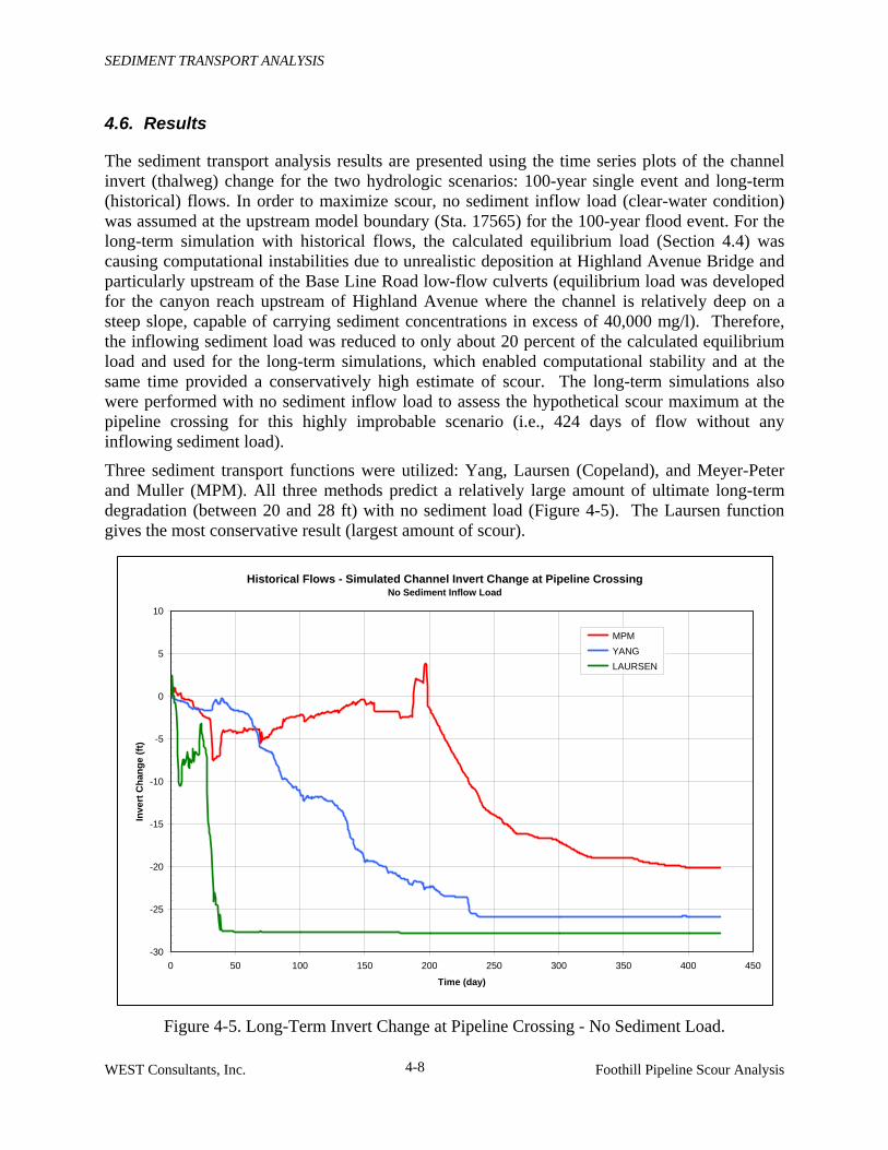
SEDIMENT TRANSPORT ANALYSIS
WEST Consultants, Inc. Foothill Pipeline Scour Analysis
4-8
Historical Flows - Simulated Channel Invert Change at Pipeline CrossingNo Sediment Inflow Load
-30
-25
-20
-15
-10
-5
0
5
10
0 50 100 150 200 250 300 350 400 450
Time (day)
Inv
ert
Ch
an
ge
(ft
)
MPM
YANG
LAURSEN
4.6. Results
The sediment transport analysis results are presented using the time series plots of the channel invert (thalweg) change for the two hydrologic scenarios: 100-year single event and long-term (historical) flows. In order to maximize scour, no sediment inflow load (clear-water condition) was assumed at the upstream model boundary (Sta. 17565) for the 100-year flood event. For the long-term simulation with historical flows, the calculated equilibrium load (Section 4.4) was causing computational instabilities due to unrealistic deposition at Highland Avenue Bridge and particularly upstream of the Base Line Road low-flow culverts (equilibrium load was developed for the canyon reach upstream of Highland Avenue where the channel is relatively deep on a steep slope, capable of carrying sediment concentrations in excess of 40,000 mg/l). Therefore, the inflowing sediment load was reduced to only about 20 percent of the calculated equilibrium load and used for the long-term simulations, which enabled computational stability and at the same time provided a conservatively high estimate of scour. The long-term simulations also were performed with no sediment inflow load to assess the hypothetical scour maximum at the pipeline crossing for this highly improbable scenario (i.e., 424 days of flow without any inflowing sediment load).
Three sediment transport functions were utilized: Yang, Laursen (Copeland), and Meyer-Peter and Muller (MPM). All three methods predict a relatively large amount of ultimate long-term degradation (between 20 and 28 ft) with no sediment load (Figure 4-5). The Laursen function gives the most conservative result (largest amount of scour).
Figure 4-5. Long-Term Invert Change at Pipeline Crossing - No Sediment Load.

SEDIMENT TRANSPORT ANALYSIS
WEST Consultants, Inc. Foothill Pipeline Scour Analysis
4-9
Historical Flows - Simulated Channel Invert Change at Pipeline Crossing20% of Equilibrium Sediment Inflow Load
-25
-20
-15
-10
-5
0
5
0 50 100 150 200 250 300 350 400 450
Time (day)
Inve
rt C
han
ge
(ft
)
MPM
YANG
For a more realistic scenario with 20 percent of equilibrium sediment load (Figure 4-6), the Laursen method failed to produce a computationally stable solution. The MPM method experienced unrealistic deposition at the upstream boundary and predicted more scour with the sediment inflow load than for clear-water conditions (this result is questionable). It appears that the Yang transport function provides the physically most realistic result for this scenario.
Figure 4-6. Long-Term Invert Change at Pipeline Crossing – 20% of Equilibrium Sediment Load (Laursen Method Failed to Provide Stable Solution).
For the 100-year single flood event (Figure 4-7), the Yang transport function surprisingly does not predict any significant scour. The MPM formulation shows degradation of 1.5 ft at the end of the flood. The Laursen method gives the most conservative prediction of 7.5 feet of scour.
It should be noted that several levels of conservatism are reflected in the above scour results: 1) All the simulations were carried out neglecting the presence of large boulders that the District placed on the downstream side of the pipeline to help prevent further erosion. This was done in case the boulders are washed away as it was the case in the past; 2) The erosion limits were fixed in place (approximately at the bank stations corresponding to the channel-forming discharge) during simulations, which also maximizes scour. In reality, large channel degradation predicted by the model would cause exceedence of the maximum stable bank height, which would lead to mass failure and lateral bankline retreat; 3) Sediment samples taken in the field are generally skewed toward sand particle sizes, neglecting the observed larger material that would likely provide additional armoring of the channel bed; 4) Roughness coefficients for sand-bed used in the model are relatively low and do not account for increased resistance by larger bed material.

SEDIMENT TRANSPORT ANALYSIS
WEST Consultants, Inc. Foothill Pipeline Scour Analysis
4-10
100-Year Storm Event - Simulated Channel Invert Change at Pipeline CrossingNo Sediment Inflow Load
-8.0
-7.0
-6.0
-5.0
-4.0
-3.0
-2.0
-1.0
0.0
1.0
0:00 2:00 4:00 6:00 8:00 10:00 12:00 14:00 16:00 18:00 20:00
Time (hour)
Inv
ert
Ch
an
ge
(ft
) MPM
YANG
LAURSEN
Figure 4-7. 100-Year Flood Invert Change at Pipeline Crossing - No Sediment Load.
4.7. Local Scour Two local scour components also were considered in addition to the long-term channel degradation and 100-year scour: 1) antidune scour that occurs in steep, sand-bed channels during high flows (passage of antidunes past a point in the channel can increase the magnitude of scour); 2) potential channel incision during low-flows. The antidune scour is generally determined as one-half the antidune height which can be estimated as follows (RCE, 1994):
2280 Ra yFh π= . < y Where: ha = antidune height y = hydraulic depth of flow FR = Froude number = 1.0 (assuming subcritical flow)

SEDIMENT TRANSPORT ANALYSIS
WEST Consultants, Inc. Foothill Pipeline Scour Analysis
4-11
The antidune scour was estimated for the 100-year flood peak (10,500 cfs) and the maximum flow in the historical flow record (3,400 cfs). The antidune scour corresponding to these two discharges is given in Table 4-2. The low-flow channel incision is estimated at 2.0 ft.
Table 4-2. Estimated Antidune Scour.
Discharge (cfs) Depth y (ft) Antidune Height ha (ft) Scour (ft) 3,400 5 4.4 2.5
10,500 10 8.8 4.5
4.8. Total Scour Total scour is found as a combination of the long-term degradation or the single storm event scour and local scour components. The results are summarized in Table 4-3 (rounded up to the nearest foot). The sediment transport model scour (Degradation) is based on the Yang function for the long-term scenario, and on the Laursen (Copeland) function for the 100-year flood. The amount of scour in scenario 1 is the anticipated ultimate scour at the pipeline crossing using historical flow conditions if no scour mitigation alternative is in place. The predicted scour in scenario 2 is the maximum scour that may be expected during the 100-year flood event in any given year (having a 1 percent chance of being equaled or exceeded) if no scour protection is in place.
Table 4-3. Total Predicted Scour at Pipeline Crossing.
Scenario/Scour Degradation (ft) Antidune (ft) Low-Flow Incision (ft) Total (ft) 1) Long-Term 15.0 2.5 2.0 20.0
2) 100-Year Flood 7.5 4.5 2.0 14.0

REFERENCES
WEST Consultants, Inc. Foothill Pipeline Scour Analysis
5-1
5. References
Flood Emergency Management Agency (FEMA). Flood Insurance Study, San Bernardino County, California, and Incorporated Areas, August 28, 2008.
Hydrologic Engineering Center (HEC). HEC-GeoRAS – GIS Tools for support of HEC-RAS using ArcGIS– User’s Manual. Version 4, U.S. Army Corps of Engineers, Hydrologic Engineering Center, Davis, California, September 2005.
Hydrologic Engineering Center (HEC). HEC-RAS River Analysis System – User’s Manual. Version 4.0, U.S. Army Corps of Engineers, Hydrologic Engineering Center, Davis, California, March 2008.
National Geodetic Survey (NGS). VERTCON - North American Vertical Datum Conversion Utility, http://www.ngs.noaa.gov/TOOLS/Vertcon/vertcon.html, 2003.
Tetra Tech (2008). City Creek Levee Hydrologic and Hydraulic Analyses, Draft Report, February 2008.
Cowan, W.L. Estimating Hydraulic Roughness Coefficients, Agricultural Engineering,
Vol. 37, No. 7, pp. 473-475, 1956.
Resource Consultants & Engineers, Inc. (RCE). Sediment and Erosion Design Guide. Prepared for Albuquerque Metropolitan Arroyo Flood Control Authority (AMAFCA), November 1994.
San Bernardino County. Hydrology Manual, August 1986. U.S. Army Corps of Engineers. SAM Hydraulic Design Package for Channels. Coastal
and Hydraulics Laboratory, U.S. Army Engineer Research and Development Center, Vicksburg, Mississippi, 2002.
WEST Consultants, Inc. FEMA Map Revision for City Creek and Plunge Creek,
September 2008. WEST Consultants, Inc. San Bernardino County FEMA Levee Certification, August
2009. Williams, D.T. Selection and Predictability of Sand Transport Relations Based upon a
Numerical Index, Doctoral Dissertation, Colorado State University, Fort Collins, CO, 1995.

APPENDIX A
HEC-RAS Hydraulic Model Results
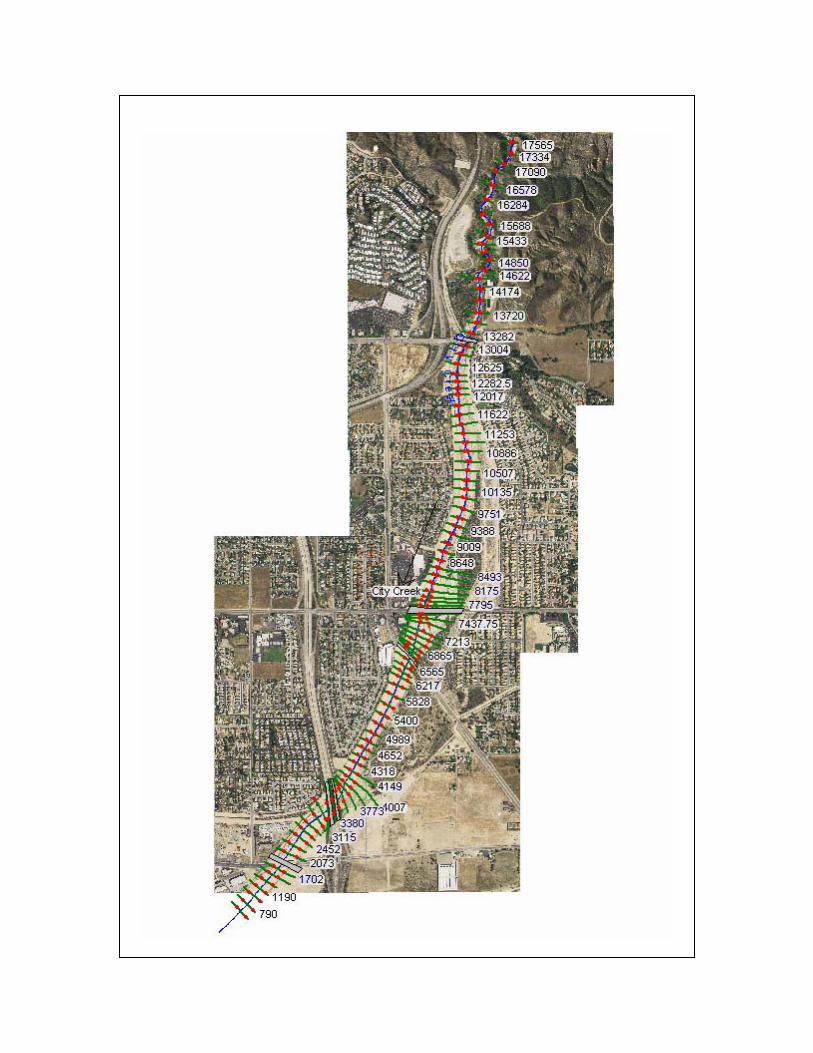

10000 12000 14000 16000
1300
1350
1400
1450
1500
1550
1600
City Creek Plan: 100-yr Steady RAS 12/22/2008
Main Channel Distance (ft)
Ele
va
tio
n (
ft)
Legend
WS Profile
Crit Profile
Ground
86
48
88
25
90
09
92
22
93
88
95
55
97
51
99
62
10
13
5
10
31
5
10
50
7
10
68
6
10
88
6
11
07
8
11
25
3
11
43
7
11
62
2
11
81
1
12
01
71
21
41
12
28
2.5
12
42
4
12
62
5
12
82
7
13
00
4
13
10
0 H
igh
lan
d A
ve
nu
e B
rid
ge
13
51
3
13
72
0
13
94
9
14
17
4
14
38
5
14
62
2
14
85
0
15
04
1
15
22
8
15
43
3
15
68
8
15
94
8
16
28
4
16
57
8
16
86
7
17
09
0
17
33
4
17
56
5
City Creek City Creek

2000 4000 6000 80001100
1150
1200
1250
1300
1350
1400
City Creek Plan: 100-yr Steady RAS 12/22/2008
Main Channel Distance (ft)
Ele
va
tio
n (
ft)
Legend
WS Profile
Crit Profile
Ground
60
0
79
0
99
9
11
90
13
78
15
59
17
02
18
00
5th
Ave
nu
e B
rid
ge
20
73
22
58
24
52
26
23
27
78
29
69
31
15
32
44
33
80
36
47
37
73
40
07
41
49
43
18
44
77
46
52
48
12
49
89
52
03
54
00
56
07
58
28
60
47
62
17
64
47
66
00
Bo
uld
er
Ave
nu
e E
xis
tin
g B
rid
ge
68
65
69
93
72
13
73
62
.5
75
13
76
00
Ba
se
line
Ave
nu
e7
79
5
80
10
81
75
83
43
84
93
86
48
88
25
90
09
92
22
93
88
95
55
City Creek City Creek

HEC-RAS Plan: 100-yr Steady River: City Creek Reach: City Creek Profile: Profile
Reach River Sta Q Total Min Ch El W.S. Elev Crit W.S. E.G. Elev E.G. Slope Vel Chnl Flow Area Top Width Froude # Chl
(cfs) (ft) (ft) (ft) (ft) (ft/ft) (ft/s) (sq ft) (ft)
City Creek 17565 10470.00 1614.00 1625.55 1625.55 1628.87 0.009589 15.32 797.05 132.79 0.91
City Creek 17334 10470.00 1603.00 1615.27 1615.27 1619.15 0.009320 16.40 727.44 103.20 0.91
City Creek 17090 10470.00 1588.00 1604.64 1603.32 1608.14 0.006243 15.68 779.04 87.61 0.76
City Creek 16867 10470.00 1584.00 1600.83 1600.83 1606.25 0.009423 19.36 618.62 63.97 0.91
City Creek 16578 10470.00 1574.73 1586.99 1586.99 1590.70 0.009662 16.12 747.08 109.73 0.91
City Creek 16284 10470.00 1568.41 1580.07 1580.07 1583.66 0.009491 15.77 757.93 118.32 0.91
City Creek 15948 10470.00 1557.51 1570.18 1570.18 1574.09 0.009108 16.50 734.40 107.23 0.90
City Creek 15688 10470.00 1552.50 1562.55 1562.55 1565.55 0.010423 14.50 820.97 146.66 0.93
City Creek 15433 10470.00 1546.37 1556.12 1556.12 1559.32 0.010738 14.71 776.71 131.65 0.94
City Creek 15228 10470.00 1530.90 1541.55 1541.55 1544.11 0.008665 13.78 946.88 193.86 0.85
City Creek 15041 10470.00 1522.91 1533.98 1533.98 1537.20 0.009383 15.03 814.25 143.72 0.90
City Creek 14850 10470.00 1516.00 1531.07 1531.07 1535.13 0.008602 16.99 737.23 103.89 0.88
City Creek 14622 10470.00 1508.88 1519.54 1519.54 1522.97 0.010307 15.21 753.02 120.25 0.93
City Creek 14385 10470.00 1493.63 1504.37 1504.37 1507.43 0.009392 14.78 839.77 151.60 0.90
City Creek 14174 10470.00 1486.98 1499.28 1499.28 1503.03 0.009197 16.21 750.05 112.17 0.90
City Creek 13949 10470.00 1480.96 1491.35 1491.35 1495.04 0.010156 15.74 723.66 108.36 0.94
City Creek 13720 10470.00 1473.94 1484.07 1484.07 1487.82 0.010332 15.84 717.27 106.80 0.95
City Creek 13513 10470.00 1457.30 1469.60 1469.60 1474.25 0.005685 17.66 647.32 76.60 0.95
City Creek 13282 10470.00 1455.71 1465.79 1465.03 1468.39 0.004078 13.21 879.22 144.59 0.79
City Creek 13100 Bridge
City Creek 13004 10470.00 1453.41 1461.20 1461.20 1464.58 0.006851 14.80 722.64 112.77 0.99
City Creek 12827 10470.00 1440.71 1453.04 1453.04 1457.06 0.004778 16.36 713.88 106.16 0.88
City Creek 12625 10470.00 1431.64 1444.27 1444.27 1448.52 0.005768 16.90 680.84 89.75 0.94
City Creek 12424 10470.00 1427.68 1436.41 1436.41 1439.90 0.006578 15.10 719.62 110.11 0.98
City Creek 12282.5 10470.00 1422.64 1432.54 1432.54 1436.38 0.006089 15.93 697.94 100.13 0.96
City Creek 12141 10470.00 1417.59 1429.27 1429.27 1433.29 0.005259 16.55 716.68 100.47 0.91
City Creek 12017 10470.00 1416.21 1427.56 1427.56 1431.18 0.005212 16.15 772.32 112.43 0.90
City Creek 11811 10470.00 1403.71 1417.48 1417.48 1422.35 0.005574 18.23 650.10 76.16 0.90
City Creek 11622 10470.00 1398.35 1412.20 1412.20 1416.25 0.004976 17.05 742.50 110.59 0.85
City Creek 11437 10470.00 1394.03 1407.73 1407.73 1412.06 0.005218 17.70 742.42 110.44 0.88
City Creek 11253 10470.00 1388.51 1401.78 1401.78 1405.82 0.004875 17.13 769.94 118.31 0.87
City Creek 11078 10470.00 1385.37 1397.88 1397.88 1401.44 0.004878 15.67 786.66 131.79 0.86
City Creek 10886 10470.00 1378.20 1387.81 1387.81 1391.50 0.006023 15.66 717.37 105.95 0.96
City Creek 10686 10470.00 1372.70 1384.86 1384.86 1389.45 0.005572 17.56 654.59 79.88 0.93
City Creek 10507 10470.00 1368.59 1380.77 1380.77 1384.88 0.005376 16.74 713.28 102.17 0.90
City Creek 10315 10470.00 1364.66 1374.20 1374.20 1378.23 0.006463 16.19 665.88 89.73 0.97
City Creek 10135 10470.00 1360.69 1372.41 1372.41 1376.61 0.005799 16.76 677.76 89.25 0.94
City Creek 9962 10470.00 1356.62 1367.09 1367.09 1370.96 0.006312 15.93 686.80 95.57 0.96
City Creek 9751 10470.00 1352.41 1362.43 1362.43 1366.13 0.005753 15.71 724.94 108.87 0.93
City Creek 9555 10470.00 1346.87 1355.11 1355.11 1358.65 0.006456 15.19 716.06 111.20 0.97
City Creek 9388 10470.00 1343.10 1350.26 1350.26 1353.25 0.007116 13.91 763.17 131.67 0.99
City Creek 9222 10470.00 1337.82 1346.52 1346.52 1349.94 0.006121 15.04 742.50 119.00 0.95
City Creek 9009 10470.00 1332.30 1340.93 1340.93 1344.67 0.006572 15.62 691.78 97.82 0.98
City Creek 8825 10470.00 1324.92 1336.14 1336.14 1339.94 0.006608 15.74 689.10 96.97 0.98
City Creek 8648 10470.00 1319.96 1331.44 1331.44 1335.26 0.005852 15.88 705.91 104.48 0.94
City Creek 8493 10470.00 1316.00 1327.15 1327.15 1331.13 0.005707 16.19 694.82 101.80 0.92
City Creek 8343 10470.00 1312.82 1322.44 1322.44 1326.61 0.006277 16.54 667.35 89.29 0.97
City Creek 8175 10470.00 1305.94 1316.82 1316.82 1320.93 0.006680 16.32 654.57 84.99 0.98
City Creek 8010 10470.00 1300.96 1312.81 1310.13 1314.54 0.002706 10.55 992.11 114.24 0.63
City Creek 7878 10470.00 1297.92 1313.46 1306.54 1314.03 0.000660 6.08 1803.18 470.25 0.32
City Creek 7795 10470.00 1295.97 1313.42 1305.10 1313.97 0.000646 5.99 1836.96 498.96 0.32
City Creek 7691 10470.00 1293.95 1313.50 1305.90 1313.86 0.000482 5.39 3021.31 733.50 0.28
City Creek 7600 Culvert
City Creek 7513 10470.00 1290.30 1302.66 1302.66 1307.02 0.005459 17.06 673.27 89.21 0.92
City Creek 7437.75 10470.00 1286.64 1294.38 1294.38 1297.38 0.007092 13.96 764.96 136.22 0.99
City Creek 7362.5 10470.00 1282.90 1288.81 1288.81 1291.03 0.007651 12.03 892.60 216.52 0.98
City Creek 7213 10470.00 1277.86 1283.71 1283.71 1285.26 0.005591 10.59 1213.39 394.98 0.85
City Creek 7111 10470.00 1275.91 1281.37 1281.37 1282.84 0.008137 10.14 1138.38 383.09 0.96
City Creek 6993 10470.00 1275.87 1280.16 1279.73 1281.25 0.005579 8.46 1281.58 399.70 0.80
City Creek 6865 10470.00 1273.89 1279.68 1278.72 1280.64 0.003679 7.87 1348.12 328.89 0.67
City Creek 6789 10470.00 1272.98 1279.47 1278.31 1280.36 0.003196 7.60 1393.75 323.56 0.63
City Creek 6721 10470.00 1272.91 1279.50 1277.57 1280.11 0.001832 6.29 1677.69 336.64 0.49
City Creek 6600 Bridge
City Creek 6565 10470.00 1268.00 1273.83 1273.83 1275.63 0.007728 11.00 1018.68 294.73 0.97
City Creek 6447 10470.00 1265.86 1271.16 1271.16 1273.11 0.007634 11.34 968.07 256.11 0.97
City Creek 6320 10470.00 1263.34 1268.44 1268.44 1270.34 0.007606 11.26 990.65 272.83 0.97
City Creek 6217 10470.00 1260.86 1266.57 1266.57 1268.43 0.007831 11.08 992.15 277.18 0.97
City Creek 6047 10470.00 1257.73 1263.65 1263.65 1265.45 0.007797 11.20 1032.46 297.35 0.97
City Creek 5828 10470.00 1253.90 1259.70 1259.70 1261.63 0.007572 11.60 996.97 264.17 0.97
City Creek 5607 10470.00 1249.51 1255.86 1255.86 1258.02 0.007783 11.87 902.35 215.10 0.99
City Creek 5400 10470.00 1245.45 1253.15 1253.15 1255.75 0.007294 13.07 839.93 180.38 0.99
City Creek 5203 10470.00 1240.83 1249.00 1249.00 1251.53 0.006567 13.06 868.67 180.94 0.95
City Creek 4989 10470.00 1236.92 1244.69 1244.69 1247.24 0.006528 13.18 871.88 181.12 0.95
City Creek 4812 10470.00 1234.00 1242.57 1242.57 1245.30 0.005983 13.72 860.08 168.00 0.93
City Creek 4652 10470.00 1230.86 1239.18 1239.18 1241.61 0.007247 12.67 865.06 186.91 0.98

HEC-RAS Plan: 100-yr Steady River: City Creek Reach: City Creek Profile: Profile (Continued)
Reach River Sta Q Total Min Ch El W.S. Elev Crit W.S. E.G. Elev E.G. Slope Vel Chnl Flow Area Top Width Froude # Chl
(cfs) (ft) (ft) (ft) (ft) (ft/ft) (ft/s) (sq ft) (ft)
City Creek 4477 10470.00 1229.00 1236.26 1236.26 1238.73 0.007286 12.73 855.63 183.66 0.98
City Creek 4318 10470.00 1226.90 1233.76 1233.76 1235.98 0.007008 12.16 917.28 218.23 0.95
City Creek 4149 10470.00 1223.97 1231.26 1231.26 1233.26 0.007668 11.55 957.84 247.73 0.98
City Creek 4007 10470.00 1223.80 1228.70 1228.70 1229.87 0.006945 9.69 1400.84 580.12 0.90
City Creek 3885 10470.00 1220.99 1226.61 1226.61 1227.73 0.006527 9.59 1464.53 622.40 0.88
City Creek 3773 10470.00 1219.95 1225.21 1225.21 1226.62 0.007246 9.86 1208.01 467.99 0.92
City Creek 3647 10470.00 1217.95 1223.39 1223.39 1224.89 0.007619 10.23 1156.26 407.24 0.94
City Creek 3498 10470.00 1215.91 1222.31 1221.23 1223.13 0.003176 7.29 1483.21 389.95 0.62
City Creek 3470 Bridge
City Creek 3380 10470.00 1214.79 1220.74 1219.60 1221.50 0.002685 7.32 1649.80 446.83 0.59
City Creek 3350 10470.00 1213.80 1220.71 1219.35 1221.40 0.002299 6.95 1671.29 394.98 0.55
City Creek 3340 Bridge
City Creek 3244 10470.00 1212.74 1217.48 1217.48 1218.98 0.007606 10.01 1126.32 385.92 0.94
City Creek 3115 10470.00 1211.00 1215.99 1215.99 1217.61 0.008725 10.26 1035.34 324.32 0.99
City Creek 2969 10470.00 1210.00 1214.28 1214.28 1215.96 0.008644 10.46 1026.72 319.70 1.00
City Creek 2778 10470.00 1208.00 1212.46 1212.45 1214.14 0.008872 10.41 1011.11 309.22 1.00
City Creek 2623 10470.00 1207.00 1211.28 1211.11 1212.85 0.007365 10.08 1047.12 300.66 0.93
City Creek 2452 10470.00 1205.79 1210.16 1209.85 1211.65 0.006478 9.82 1078.83 312.76 0.88
City Creek 2258 10470.00 1204.12 1208.64 1208.47 1210.31 0.007202 10.42 1025.04 282.56 0.93
City Creek 2073 10470.00 1203.00 1208.57 1206.97 1209.33 0.002351 7.00 1530.26 327.85 0.55
City Creek 1800 Bridge
City Creek 1702 10470.00 1200.93 1206.56 1205.27 1207.75 0.003320 8.76 1200.90 226.87 0.66
City Creek 1559 10470.00 1199.95 1204.79 1204.79 1206.96 0.007573 11.94 909.83 219.43 0.98
City Creek 1378 10470.00 1198.57 1203.13 1202.63 1204.59 0.005547 9.73 1089.43 266.26 0.83
City Creek 1190 10470.00 1197.38 1201.91 1201.60 1203.47 0.006396 10.03 1056.08 275.66 0.88
City Creek 999 10470.00 1196.48 1201.07 1200.42 1202.32 0.004836 8.99 1186.61 301.77 0.77
City Creek 790 10470.00 1195.18 1200.20 1199.36 1201.35 0.004183 8.65 1231.35 298.02 0.72
City Creek 600 10470.00 1194.27 1198.90 1198.54 1200.38 0.006006 9.82 1095.36 290.93 0.86
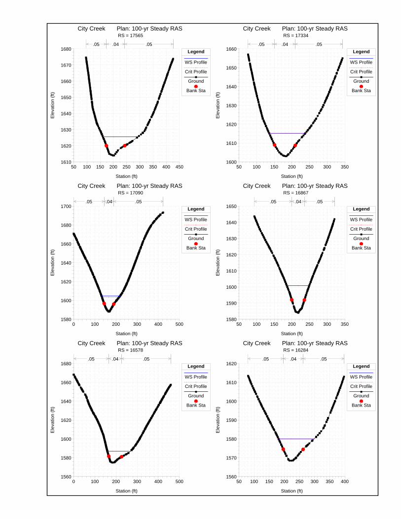
50 100 150 200 250 300 350 400 4501610
1620
1630
1640
1650
1660
1670
1680
City Creek Plan: 100-yr Steady RAS RS = 17565
Station (ft)
Ele
va
tio
n (
ft)
Legend
WS Profile
Crit Profile
Ground
Bank Sta
.05 .04 .05
50 100 150 200 250 300 3501600
1610
1620
1630
1640
1650
1660
City Creek Plan: 100-yr Steady RAS RS = 17334
Station (ft)
Ele
va
tio
n (
ft)
Legend
WS Profile
Crit Profile
Ground
Bank Sta
.05 .04 .05
0 100 200 300 400 5001580
1600
1620
1640
1660
1680
1700
City Creek Plan: 100-yr Steady RAS RS = 17090
Station (ft)
Ele
va
tio
n (
ft)
Legend
WS Profile
Crit Profile
Ground
Bank Sta
.05 .04 .05
50 100 150 200 250 300 3501580
1590
1600
1610
1620
1630
1640
1650
City Creek Plan: 100-yr Steady RAS RS = 16867
Station (ft)
Ele
va
tio
n (
ft)
Legend
WS Profile
Crit Profile
Ground
Bank Sta
.05 .04 .05
0 100 200 300 400 5001560
1580
1600
1620
1640
1660
1680
City Creek Plan: 100-yr Steady RAS RS = 16578
Station (ft)
Ele
va
tio
n (
ft)
Legend
WS Profile
Crit Profile
Ground
Bank Sta
.05 .04 .05
50 100 150 200 250 300 350 4001560
1570
1580
1590
1600
1610
1620
City Creek Plan: 100-yr Steady RAS RS = 16284
Station (ft)
Ele
va
tio
n (
ft)
Legend
WS Profile
Crit Profile
Ground
Bank Sta
.05 .04 .05

0 50 100 150 200 250 300 3501550
1560
1570
1580
1590
1600
City Creek Plan: 100-yr Steady RAS RS = 15948
Station (ft)
Ele
va
tio
n (
ft)
Legend
WS Profile
Crit Profile
Ground
Bank Sta
.05 .04 .05
50 100 150 200 250 300 350 400 4501550
1560
1570
1580
1590
1600
City Creek Plan: 100-yr Steady RAS RS = 15688
Station (ft)
Ele
va
tio
n (
ft)
Legend
WS Profile
Crit Profile
Ground
Bank Sta
.05 .04 .05
100 200 300 400 5001540
1550
1560
1570
1580
1590
City Creek Plan: 100-yr Steady RAS RS = 15433
Station (ft)
Ele
va
tio
n (
ft)
Legend
WS Profile
Crit Profile
Ground
Bank Sta
.05 .04 .05
0 100 200 300 400 500 6001530
1540
1550
1560
1570
1580
1590
City Creek Plan: 100-yr Steady RAS RS = 15228
Station (ft)
Ele
va
tio
n (
ft)
Legend
WS Profile
Crit Profile
Ground
Bank Sta
.05 .04 .05
0 100 200 300 400 5001520
1530
1540
1550
1560
1570
City Creek Plan: 100-yr Steady RAS RS = 15041
Station (ft)
Ele
va
tio
n (
ft)
Legend
WS Profile
Crit Profile
Ground
Bank Sta
.05 .04 .05
50 100 150 200 250 300 350 4001510
1520
1530
1540
1550
1560
1570
City Creek Plan: 100-yr Steady RAS RS = 14850
Station (ft)
Ele
va
tio
n (
ft)
Legend
WS Profile
Crit Profile
Ground
Bank Sta
.05 .04 .05

0 50 100 150 200 250 300 350 4001500
1510
1520
1530
1540
1550
1560
City Creek Plan: 100-yr Steady RAS RS = 14622
Station (ft)
Ele
va
tio
n (
ft)
Legend
WS Profile
Crit Profile
Ground
Bank Sta
.05 .04 .05
0 100 200 300 400 500 600 7001490
1495
1500
1505
1510
1515
1520
1525
1530
City Creek Plan: 100-yr Steady RAS RS = 14385
Station (ft)
Ele
va
tio
n (
ft)
Legend
WS Profile
Crit Profile
Ground
Bank Sta
.05 .04 .05
50 100 150 200 250 300 3501485
1490
1495
1500
1505
1510
1515
City Creek Plan: 100-yr Steady RAS RS = 14174
Station (ft)
Ele
va
tio
n (
ft)
Legend
WS Profile
Crit Profile
Ground
Bank Sta
.05 .04 .05
50 100 150 200 250 300 3501480
1485
1490
1495
1500
1505
City Creek Plan: 100-yr Steady RAS RS = 13949
Station (ft)
Ele
va
tio
n (
ft)
Legend
WS Profile
Crit Profile
Ground
Bank Sta
.05 .04 .05
0 100 200 300 400 5001470
1475
1480
1485
1490
1495
1500
1505
City Creek Plan: 100-yr Steady RAS RS = 13720
Station (ft)
Ele
va
tio
n (
ft)
Legend
WS Profile
Crit Profile
Ground
Bank Sta
.05 .04 .05
0 100 200 300 400 5001455
1460
1465
1470
1475
1480
1485
1490
City Creek Plan: 100-yr Steady RAS RS = 13513
Station (ft)
Ele
va
tio
n (
ft)
Legend
WS Profile
Crit Profile
Ground
Bank Sta
.04 .03 .04

0 100 200 300 4001455
1460
1465
1470
1475
1480
1485
City Creek Plan: 100-yr Steady RAS RS = 13282
Station (ft)
Ele
va
tio
n (
ft)
Legend
WS Profile
Crit Profile
Ground
Bank Sta
.04 .03 .04
0 100 200 300 400 500 6001450
1460
1470
1480
1490
1500
City Creek Plan: 100-yr Steady RAS RS = 13100 BR Highland Avenue Bridge
Station (ft)
Ele
va
tio
n (
ft)
Legend
WS Profile
Crit Profile
Ground
Bank Sta
.015
0 100 200 300 400 500 6001450
1460
1470
1480
1490
1500
1510
City Creek Plan: 100-yr Steady RAS RS = 13100 BR Highland Avenue Bridge
Station (ft)
Ele
va
tio
n (
ft)
Legend
WS Profile
Crit Profile
Ground
Bank Sta
.015
0 100 200 300 400 500 6001450
1460
1470
1480
1490
1500
1510
City Creek Plan: 100-yr Steady RAS RS = 13004
Station (ft)
Ele
va
tio
n (
ft)
Legend
WS Profile
Crit Profile
Ground
Bank Sta
.04 .03 .04
0 50 100 150 200 250 300 3501440
1450
1460
1470
1480
1490
City Creek Plan: 100-yr Steady RAS RS = 12827
Station (ft)
Ele
va
tio
n (
ft)
Legend
WS Profile
Crit Profile
Ground
Bank Sta
.04 .03 .04
0 100 200 300 400 5001430
1435
1440
1445
1450
1455
1460
1465
1470
City Creek Plan: 100-yr Steady RAS RS = 12625
Station (ft)
Ele
va
tio
n (
ft)
Legend
WS Profile
Crit Profile
Ground
Bank Sta
.04 .03 .04

0 100 200 300 400 500 6001425
1430
1435
1440
1445
1450
1455
1460
City Creek Plan: 100-yr Steady RAS RS = 12424
Station (ft)
Ele
va
tio
n (
ft)
Legend
WS Profile
Crit Profile
Ground
Bank Sta
.04 .03 .04
0 100 200 300 400 5001420
1425
1430
1435
1440
1445
1450
1455
City Creek Plan: 100-yr Steady RAS RS = 12282.5
Station (ft)
Ele
va
tio
n (
ft)
Legend
WS Profile
Crit Profile
Ground
Bank Sta
.04 .03 .04
0 100 200 300 400 5001415
1420
1425
1430
1435
1440
1445
1450
1455
City Creek Plan: 100-yr Steady RAS RS = 12141
Station (ft)
Ele
va
tio
n (
ft)
Legend
WS Profile
Crit Profile
Ground
Bank Sta
.04 .03 .04
100 200 300 400 500 6001415
1420
1425
1430
1435
1440
1445
1450
City Creek Plan: 100-yr Steady RAS RS = 12017
Station (ft)
Ele
va
tio
n (
ft)
Legend
WS Profile
Crit Profile
Ground
Bank Sta
.04 .03 .04
100 200 300 400 500 6001400
1405
1410
1415
1420
1425
1430
1435
1440
1445
City Creek Plan: 100-yr Steady RAS RS = 11811
Station (ft)
Ele
va
tio
n (
ft)
Legend
WS Profile
Crit Profile
Ground
Bank Sta
.04 .03 .04
0 100 200 300 400 500 6001390
1400
1410
1420
1430
1440
1450
City Creek Plan: 100-yr Steady RAS RS = 11622
Station (ft)
Ele
va
tio
n (
ft)
Legend
WS Profile
Crit Profile
Ground
Bank Sta
.04 .03
.04

0 100 200 300 400 500 6001390
1400
1410
1420
1430
1440
City Creek Plan: 100-yr Steady RAS RS = 11437
Station (ft)
Ele
va
tio
n (
ft)
Legend
WS Profile
Crit Profile
Ground
Bank Sta
.04 .03
.04
0 100 200 300 400 500 6001385
1390
1395
1400
1405
1410
1415
1420
1425
1430
City Creek Plan: 100-yr Steady RAS RS = 11253
Station (ft)
Ele
va
tio
n (
ft)
Legend
WS Profile
Crit Profile
Ground
Bank Sta
.04 .03
.04
0 100 200 300 400 500 6001380
1390
1400
1410
1420
1430
City Creek Plan: 100-yr Steady RAS RS = 11078
Station (ft)
Ele
va
tio
n (
ft)
Legend
WS Profile
Crit Profile
Ground
Bank Sta
.04 .03 .04
0 100 200 300 400 500 6001375
1380
1385
1390
1395
1400
1405
1410
1415
City Creek Plan: 100-yr Steady RAS RS = 10886
Station (ft)
Ele
va
tio
n (
ft)
Legend
WS Profile
Crit Profile
Ground
Bank Sta
.04 .03 .04
0 100 200 300 400 500 6001370
1375
1380
1385
1390
1395
1400
1405
1410
City Creek Plan: 100-yr Steady RAS RS = 10686
Station (ft)
Ele
va
tio
n (
ft)
Legend
WS Profile
Crit Profile
Ground
Bank Sta
.04 .03 .04
0 100 200 300 400 5001365
1370
1375
1380
1385
1390
1395
1400
1405
City Creek Plan: 100-yr Steady RAS RS = 10507
Station (ft)
Ele
va
tio
n (
ft)
Legend
WS Profile
Crit Profile
Ground
Bank Sta
.04 .03 .04

0 100 200 300 400 500 6001360
1365
1370
1375
1380
1385
1390
1395
1400
City Creek Plan: 100-yr Steady RAS RS = 10315
Station (ft)
Ele
va
tio
n (
ft)
Legend
WS Profile
Crit Profile
Ground
Bank Sta
.04 .03 .04
0 100 200 300 400 5001360
1365
1370
1375
1380
1385
1390
1395
City Creek Plan: 100-yr Steady RAS RS = 10135
Station (ft)
Ele
va
tio
n (
ft)
Legend
WS Profile
Crit Profile
Ground
Bank Sta
.04 .03 .04
0 100 200 300 400 5001355
1360
1365
1370
1375
1380
1385
1390
City Creek Plan: 100-yr Steady RAS RS = 9962
Station (ft)
Ele
va
tio
n (
ft)
Legend
WS Profile
Crit Profile
Ground
Bank Sta
.04 .03 .04
0 100 200 300 400 5001350
1355
1360
1365
1370
1375
1380
1385
City Creek Plan: 100-yr Steady RAS RS = 9751
Station (ft)
Ele
va
tio
n (
ft)
Legend
WS Profile
Crit Profile
Ground
Bank Sta
.04 .03 .04
600 650 700 750 800 850 900 950 10001345
1350
1355
1360
1365
1370
1375
City Creek Plan: 100-yr Steady RAS RS = 9555
Station (ft)
Ele
va
tio
n (
ft)
Legend
WS Profile
Crit Profile
Ground
Bank Sta
.04 .03 .04
600 700 800 900 1000 11001340
1345
1350
1355
1360
1365
1370
City Creek Plan: 100-yr Steady RAS RS = 9388
Station (ft)
Ele
va
tio
n (
ft)
Legend
WS Profile
Crit Profile
Ground
Bank Sta
.04 .03 .04

600 700 800 900 1000 1100 12001335
1340
1345
1350
1355
1360
1365
1370
City Creek Plan: 100-yr Steady RAS RS = 9222
Station (ft)
Ele
va
tio
n (
ft)
Legend
WS Profile
Crit Profile
Ground
Bank Sta
.04 .03 .04
950 1000 1050 1100 1150 1200 12501330
1335
1340
1345
1350
1355
1360
City Creek Plan: 100-yr Steady RAS RS = 9009
Station (ft)
Ele
va
tio
n (
ft)
Legend
WS Profile
Crit Profile
Ground
Bank Sta
.04 .03 .04
900 950 1000 1050 1100 1150 1200 1250 13001320
1325
1330
1335
1340
1345
1350
1355
City Creek Plan: 100-yr Steady RAS RS = 8825
Station (ft)
Ele
va
tio
n (
ft)
Legend
WS Profile
Crit Profile
Ground
Bank Sta
.04 .03 .04
1050 1100 1150 1200 1250 1300 13501315
1320
1325
1330
1335
1340
1345
1350
City Creek Plan: 100-yr Steady RAS RS = 8648
Station (ft)
Ele
va
tio
n (
ft)
Legend
WS Profile
Crit Profile
Ground
Bank Sta
.04 .03 .04
400 600 800 1000 1200 14001315
1320
1325
1330
1335
1340
1345
1350
City Creek Plan: 100-yr Steady RAS RS = 8493
Station (ft)
Ele
va
tio
n (
ft)
Legend
WS Profile
Crit Profile
Ground
Bank Sta
.04 .03
.04
400 600 800 1000 1200 14001310
1315
1320
1325
1330
1335
1340
City Creek Plan: 100-yr Steady RAS RS = 8343
Station (ft)
Ele
va
tio
n (
ft)
Legend
WS Profile
Crit Profile
Ground
Bank Sta
.04 .03
.04

200 400 600 800 1000 1200 14001305
1310
1315
1320
1325
1330
1335
1340
City Creek Plan: 100-yr Steady RAS RS = 8175
Station (ft)
Ele
va
tio
n (
ft)
Legend
WS Profile
Crit Profile
Ground
Bank Sta
.04 .03
.04
200 400 600 800 1000 1200 14001300
1305
1310
1315
1320
1325
1330
1335
City Creek Plan: 100-yr Steady RAS RS = 8010
Station (ft)
Ele
va
tio
n (
ft)
Legend
WS Profile
Crit Profile
Ground
Bank Sta
.04 .03 .04
200 400 600 800 1000 1200 14001295
1300
1305
1310
1315
1320
1325
1330
City Creek Plan: 100-yr Steady RAS RS = 7878
Station (ft)
Ele
va
tio
n (
ft)
Legend
WS Profile
Crit Profile
Ground
Bank Sta
.04 .03 .04
200 400 600 800 1000 1200 14001295
1300
1305
1310
1315
1320
1325
1330
City Creek Plan: 100-yr Steady RAS RS = 7795
Station (ft)
Ele
va
tio
n (
ft)
Legend
WS Profile
Crit Profile
Ground
Bank Sta
.04 .03 .04
200 400 600 800 1000 1200 14001290
1295
1300
1305
1310
1315
1320
1325
City Creek Plan: 100-yr Steady RAS RS = 7691
Station (ft)
Ele
va
tio
n (
ft)
Legend
WS Profile
Crit Profile
Ground
Bank Sta
.04 .03 .04
200 400 600 800 1000 1200 14001290
1295
1300
1305
1310
1315
1320
1325
City Creek Plan: 100-yr Steady RAS RS = 7600 Culv Baseline Avenue
Station (ft)
Ele
va
tio
n (
ft)
Legend
WS Profile
Crit Profile
Ground
Bank Sta
.04

200 400 600 800 1000 1200 14001285
1290
1295
1300
1305
1310
1315
City Creek Plan: 100-yr Steady RAS RS = 7600 Culv Baseline Avenue
Station (ft)
Ele
va
tio
n (
ft)
Legend
WS Profile
Crit Profile
Ground
Bank Sta
.04
200 400 600 800 1000 1200 14001290
1295
1300
1305
1310
1315
City Creek Plan: 100-yr Steady RAS RS = 7513
Station (ft)
Ele
va
tio
n (
ft)
Legend
WS Profile
Crit Profile
Ground
Bank Sta
.04 .03
.04
200 400 600 800 1000 1200 14001285
1290
1295
1300
1305
1310
City Creek Plan: 100-yr Steady RAS RS = 7437.75
Station (ft)
Ele
va
tio
n (
ft)
Legend
WS Profile
Crit Profile
Ground
Bank Sta
.04 .03 .04
200 400 600 800 1000 1200 14001280
1285
1290
1295
1300
1305
1310
City Creek Plan: 100-yr Steady RAS RS = 7362.5
Station (ft)
Ele
va
tio
n (
ft)
Legend
WS Profile
Crit Profile
Ground
Bank Sta
.04 .03 .04
200 400 600 800 1000 12001275
1280
1285
1290
1295
1300
1305
City Creek Plan: 100-yr Steady RAS RS = 7213
Station (ft)
Ele
va
tio
n (
ft)
Legend
WS Profile
Crit Profile
Ground
Bank Sta
.04 .03 .04
200 400 600 800 1000 12001275
1280
1285
1290
1295
1300
1305
City Creek Plan: 100-yr Steady RAS RS = 7111
Station (ft)
Ele
va
tio
n (
ft)
Legend
WS Profile
Crit Profile
Ground
Bank Sta
.04 .03 .04

400 500 600 700 800 900 1000 1100 12001275
1280
1285
1290
1295
1300
1305
City Creek Plan: 100-yr Steady RAS RS = 6993
Station (ft)
Ele
va
tio
n (
ft)
Legend
WS Profile
Crit Profile
Ground
Bank Sta
.04 .03 .04
500 600 700 800 900 1000 1100 12001270
1275
1280
1285
1290
1295
1300
City Creek Plan: 100-yr Steady RAS RS = 6865
Station (ft)
Ele
va
tio
n (
ft)
Legend
WS Profile
Crit Profile
Ground
Bank Sta
.04 .03 .04
600 700 800 900 1000 1100 1200 13001270
1275
1280
1285
1290
1295
1300
City Creek Plan: 100-yr Steady RAS RS = 6789
Station (ft)
Ele
va
tio
n (
ft)
Legend
WS Profile
Crit Profile
Ground
Bank Sta
.04 .03 .04
1500 1600 1700 1800 1900 2000 2100 22001270
1275
1280
1285
1290
1295
City Creek Plan: 100-yr Steady RAS RS = 6721
Station (ft)
Ele
va
tio
n (
ft)
Legend
WS Profile
Crit Profile
Ground
Bank Sta
.04 .03 .04
1400 1500 1600 1700 1800 1900 2000 2100 22001270
1275
1280
1285
1290
1295
City Creek Plan: 100-yr Steady RAS RS = 6600 BR Boulder Avenue Existing Bridge
Station (ft)
Ele
va
tio
n (
ft)
Legend
WS Profile
Crit Profile
Ground
Bank Sta
Pier Debris
.04 .03 .04
1400 1500 1600 1700 1800 1900 2000 21001265
1270
1275
1280
1285
1290
1295
City Creek Plan: 100-yr Steady RAS RS = 6600 BR Boulder Avenue Existing Bridge
Station (ft)
Ele
va
tio
n (
ft)
Legend
WS Profile
Crit Profile
Ground
Bank Sta
.04 .03 .04

1500 1600 1700 1800 1900 2000 21001265
1270
1275
1280
1285
1290
City Creek Plan: 100-yr Steady RAS RS = 6565
Station (ft)
Ele
va
tio
n (
ft)
Legend
WS Profile
Crit Profile
Ground
Bank Sta
.04 .03 .04
1400 1500 1600 1700 1800 1900 20001265
1270
1275
1280
1285
1290
City Creek Plan: 100-yr Steady RAS RS = 6447
Station (ft)
Ele
va
tio
n (
ft)
Legend
WS Profile
Crit Profile
Ground
Bank Sta
.04 .03 .04
1400 1500 1600 1700 1800 19001260
1265
1270
1275
1280
1285
City Creek Plan: 100-yr Steady RAS RS = 6320
Station (ft)
Ele
va
tio
n (
ft)
Legend
WS Profile
Crit Profile
Ground
Bank Sta
.04 .03 .04
1300 1400 1500 1600 1700 1800 19001260
1265
1270
1275
1280
1285
City Creek Plan: 100-yr Steady RAS RS = 6217
Station (ft)
Ele
va
tio
n (
ft)
Legend
WS Profile
Crit Profile
Ground
Bank Sta
.04 .03 .04
1300 1400 1500 1600 1700 18001255
1260
1265
1270
1275
1280
City Creek Plan: 100-yr Steady RAS RS = 6047
Station (ft)
Ele
va
tio
n (
ft)
Legend
WS Profile
Crit Profile
Ground
Bank Sta
.04 .03 .04
1200 1300 1400 1500 1600 17001250
1255
1260
1265
1270
1275
City Creek Plan: 100-yr Steady RAS RS = 5828
Station (ft)
Ele
va
tio
n (
ft)
Legend
WS Profile
Crit Profile
Ground
Bank Sta
.04 .03 .04

1250 1300 1350 1400 1450 1500 1550 16001248
1250
1252
1254
1256
1258
1260
1262
1264
1266
1268
City Creek Plan: 100-yr Steady RAS RS = 5607
Station (ft)
Ele
va
tio
n (
ft)
Legend
WS Profile
Crit Profile
Ground
Bank Sta
.04
.03 .04
1200 1250 1300 1350 1400 1450 1500 15501245
1250
1255
1260
1265
City Creek Plan: 100-yr Steady RAS RS = 5400
Station (ft)
Ele
va
tio
n (
ft)
Legend
WS Profile
Crit Profile
Ground
Bank Sta
.04 .03 .04
1100 1150 1200 1250 1300 1350 1400 14501240
1245
1250
1255
1260
1265
City Creek Plan: 100-yr Steady RAS RS = 5203
Station (ft)
Ele
va
tio
n (
ft)
Legend
WS Profile
Crit Profile
Ground
Bank Sta
.04 .03 .04
1000 1050 1100 1150 1200 1250 1300 1350 1400 14501235
1240
1245
1250
1255
1260
City Creek Plan: 100-yr Steady RAS RS = 4989
Station (ft)
Ele
va
tio
n (
ft)
Legend
WS Profile
Crit Profile
Ground
Bank Sta
.04 .03 .04
900 1000 1100 1200 1300 14001230
1235
1240
1245
1250
1255
City Creek Plan: 100-yr Steady RAS RS = 4812
Station (ft)
Ele
va
tio
n (
ft)
Legend
WS Profile
Crit Profile
Ground
Bank Sta
.04 .03 .04
1000 1050 1100 1150 1200 1250 1300 1350 14001230
1235
1240
1245
1250
1255
City Creek Plan: 100-yr Steady RAS RS = 4652
Station (ft)
Ele
va
tio
n (
ft)
Legend
WS Profile
Crit Profile
Ground
Bank Sta
.04 .03 .04

1000 1050 1100 1150 1200 1250 1300 13501225
1230
1235
1240
1245
1250
City Creek Plan: 100-yr Steady RAS RS = 4477
Station (ft)
Ele
va
tio
n (
ft)
Legend
WS Profile
Crit Profile
Ground
Bank Sta
.04 .03 .04
900 1000 1100 1200 1300 14001226
1228
1230
1232
1234
1236
1238
1240
1242
1244
City Creek Plan: 100-yr Steady RAS RS = 4318
Station (ft)
Ele
va
tio
n (
ft)
Legend
WS Profile
Crit Profile
Ground
Bank Sta
.04 .03 .04
600 700 800 900 1000 1100 1200 1300 14001220
1225
1230
1235
1240
1245
City Creek Plan: 100-yr Steady RAS RS = 4149
Station (ft)
Ele
va
tio
n (
ft)
Legend
WS Profile
Crit Profile
Ground
Bank Sta
.04 .03 .04
200 400 600 800 1000 1200 14001222
1224
1226
1228
1230
1232
1234
1236
1238
1240
1242
City Creek Plan: 100-yr Steady RAS RS = 4007
Station (ft)
Ele
va
tio
n (
ft)
Legend
WS Profile
Crit Profile
Ground
Bank Sta
.04 .03 .04
400 600 800 1000 1200 1400 16001220
1225
1230
1235
1240
1245
City Creek Plan: 100-yr Steady RAS RS = 3885
Station (ft)
Ele
va
tio
n (
ft)
Legend
WS Profile
Crit Profile
Ground
Bank Sta
.04 .03 .04
600 800 1000 1200 1400 16001215
1220
1225
1230
1235
1240
1245
City Creek Plan: 100-yr Steady RAS RS = 3773
Station (ft)
Ele
va
tio
n (
ft)
Legend
WS Profile
Crit Profile
Ground
Bank Sta
.04 .03 .04

800 900 1000 1100 1200 1300 1400 15001215
1220
1225
1230
1235
1240
1245
City Creek Plan: 100-yr Steady RAS RS = 3647
Station (ft)
Ele
va
tio
n (
ft)
Legend
WS Profile
Crit Profile
Ground
Bank Sta
.04 .03 .04
0 200 400 600 8001215
1220
1225
1230
1235
1240
1245
City Creek Plan: 100-yr Steady RAS RS = 3498
Station (ft)
Ele
va
tio
n (
ft)
Legend
WS Profile
Crit Profile
Ground
Bank Sta
.04 .03 .04
0 200 400 600 8001215
1220
1225
1230
1235
1240
1245
City Creek Plan: 100-yr Steady RAS RS = 3470 BR I-30 Northbound.
Station (ft)
Ele
va
tio
n (
ft)
Legend
WS Profile
Crit Profile
Ground
Bank Sta
.04 .03 .04
0 200 400 600 800 10001210
1215
1220
1225
1230
1235
1240
1245
City Creek Plan: 100-yr Steady RAS RS = 3470 BR I-30 Northbound.
Station (ft)
Ele
va
tio
n (
ft)
Legend
WS Profile
Crit Profile
Ground
Bank Sta
.04 .03 .04
0 200 400 600 800 10001210
1215
1220
1225
1230
1235
1240
1245
City Creek Plan: 100-yr Steady RAS RS = 3380
Station (ft)
Ele
va
tio
n (
ft)
Legend
WS Profile
Crit Profile
Ground
Bank Sta
.04 .03 .04
0 200 400 600 800 10001210
1215
1220
1225
1230
1235
1240
1245
City Creek Plan: 100-yr Steady RAS RS = 3350
Station (ft)
Ele
va
tio
n (
ft)
Legend
WS Profile
Crit Profile
Ground
Bank Sta
.04 .03 .04

0 200 400 600 800 10001210
1215
1220
1225
1230
1235
1240
1245
City Creek Plan: 100-yr Steady RAS RS = 3340 BR I-30 Southbound.
Station (ft)
Ele
va
tio
n (
ft)
Legend
WS Profile
Crit Profile
Ground
Bank Sta
.04 .03 .04
0 200 400 600 800 10001210
1215
1220
1225
1230
1235
1240
1245
City Creek Plan: 100-yr Steady RAS RS = 3340 BR I-30 Southbound.
Station (ft)
Ele
va
tio
n (
ft)
Legend
WS Profile
Crit Profile
Ground
Bank Sta
.04 .03 .04
0 200 400 600 800 10001210
1215
1220
1225
1230
1235
1240
City Creek Plan: 100-yr Steady RAS RS = 3244
Station (ft)
Ele
va
tio
n (
ft)
Legend
WS Profile
Crit Profile
Ground
Bank Sta
.04 .03 .04
0 200 400 600 8001210
1215
1220
1225
1230
1235
City Creek Plan: 100-yr Steady RAS RS = 3115
Station (ft)
Ele
va
tio
n (
ft)
Legend
WS Profile
Crit Profile
Ground
Bank Sta
.04 .03
100 200 300 400 500 600 700 8001210
1215
1220
1225
1230
1235
City Creek Plan: 100-yr Steady RAS RS = 2969
Station (ft)
Ele
va
tio
n (
ft)
Legend
WS Profile
Crit Profile
Ground
Bank Sta
.04 .03 .04
200 300 400 500 600 700 8001205
1210
1215
1220
1225
1230
1235
City Creek Plan: 100-yr Steady RAS RS = 2778
Station (ft)
Ele
va
tio
n (
ft)
Legend
WS Profile
Crit Profile
Ground
Bank Sta
.04 .03 .04

300 400 500 600 700 800 9001205
1210
1215
1220
1225
1230
City Creek Plan: 100-yr Steady RAS RS = 2623
Station (ft)
Ele
va
tio
n (
ft)
Legend
WS Profile
Crit Profile
Ground
Bank Sta
.04 .03 .04
300 400 500 600 700 800 900 10001205
1210
1215
1220
1225
City Creek Plan: 100-yr Steady RAS RS = 2452
Station (ft)
Ele
va
tio
n (
ft)
Legend
WS Profile
Crit Profile
Ground
Bank Sta
.04 .03 .04
400 500 600 700 800 900 1000 11001200
1205
1210
1215
1220
1225
City Creek Plan: 100-yr Steady RAS RS = 2258
Station (ft)
Ele
va
tio
n (
ft)
Legend
WS Profile
Crit Profile
Ground
Bank Sta
.04 .03 .04
400 500 600 700 800 900 1000 1100 12001200
1205
1210
1215
1220
1225
City Creek Plan: 100-yr Steady RAS RS = 2073
Station (ft)
Ele
va
tio
n (
ft)
Legend
WS Profile
Crit Profile
Ground
Bank Sta
.04 .03 .04
200 400 600 800 1000 12001200
1205
1210
1215
1220
1225
City Creek Plan: 100-yr Steady RAS RS = 1800 BR 5th Avenue Bridge
Station (ft)
Ele
va
tio
n (
ft)
Legend
WS Profile
Crit Profile
Ground
Bank Sta
.04 .03 .04
200 400 600 800 1000 1200 14001200
1205
1210
1215
1220
1225
City Creek Plan: 100-yr Steady RAS RS = 1800 BR 5th Avenue Bridge
Station (ft)
Ele
va
tio
n (
ft)
Legend
WS Profile
Crit Profile
Ground
Bank Sta
.04 .03 .04

500 600 700 800 900 1000 1100 1200 13001200
1205
1210
1215
1220
City Creek Plan: 100-yr Steady RAS RS = 1702
Station (ft)
Ele
va
tio
n (
ft)
Legend
WS Profile
Crit Profile
Ground
Bank Sta
.04 .03 .04
400 500 600 700 800 900 1000 1100 12001195
1200
1205
1210
1215
1220
City Creek Plan: 100-yr Steady RAS RS = 1559
Station (ft)
Ele
va
tio
n (
ft)
Legend
WS Profile
Crit Profile
Ground
Bank Sta
.04 .03 .04
300 400 500 600 700 800 9001195
1200
1205
1210
1215
1220
City Creek Plan: 100-yr Steady RAS RS = 1378
Station (ft)
Ele
va
tio
n (
ft)
Legend
WS Profile
Crit Profile
Ground
Bank Sta
.04 .03 .04
100 200 300 400 500 600 7001195
1200
1205
1210
1215
1220
City Creek Plan: 100-yr Steady RAS RS = 1190
Station (ft)
Ele
va
tio
n (
ft)
Legend
WS Profile
Crit Profile
Ground
Bank Sta
.04
.03 .04
0 100 200 300 400 500 6001196
1198
1200
1202
1204
1206
1208
1210
1212
1214
City Creek Plan: 100-yr Steady RAS RS = 999
Station (ft)
Ele
va
tio
n (
ft)
Legend
WS Profile
Crit Profile
Ground
Bank Sta
.04
.03 .04
0 100 200 300 400 500 6001195
1200
1205
1210
1215
1220
City Creek Plan: 100-yr Steady RAS RS = 790
Station (ft)
Ele
va
tio
n (
ft)
Legend
WS Profile
Crit Profile
Ground
Bank Sta
.04 .03 .04
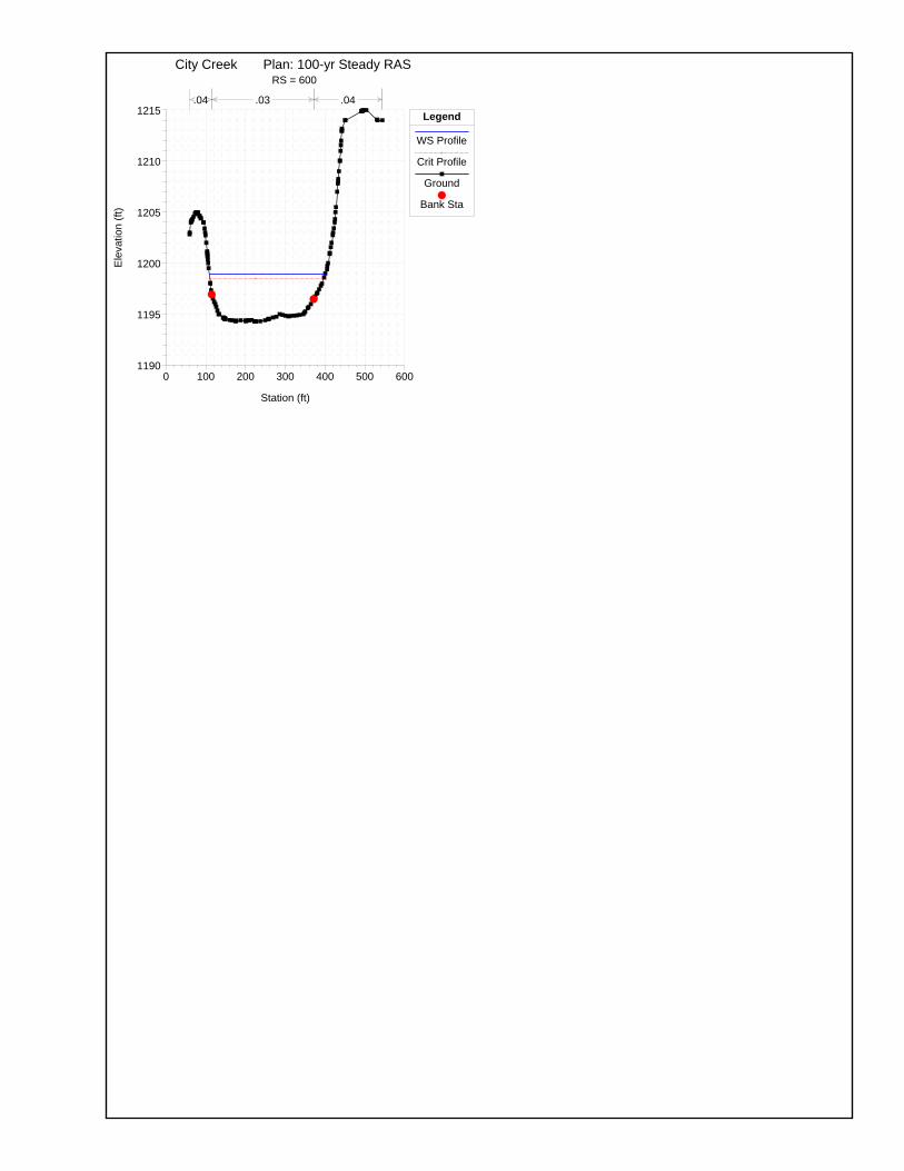
0 100 200 300 400 500 6001190
1195
1200
1205
1210
1215
City Creek Plan: 100-yr Steady RAS RS = 600
Station (ft)
Ele
va
tio
n (
ft)
Legend
WS Profile
Crit Profile
Ground
Bank Sta
.04 .03 .04
APPENDIX F-3 Upper SAR HCP Approved Covered Activities


