54
California Air Resources Board – 2017 Scoping Plan November 2017 Appendix G Alternatives Evaluation, AB 197 Estimations, and Health Impacts
California Air Resources Board – 2017 Scoping Plan November 2017
Appendix G Alternatives Evaluation, AB 197 Estimations, and Health
Impacts
California Air Resources Board – 2017 Scoping Plan November 2017
This Page Intentionally Left Blank
California Air Resources Board – 2017 Scoping Plan November 2017
i
Introduction This appendix provides additional detail on the evaluation of the four alternatives to the Scoping Plan Scenario and additional detail on the air quality and health analyses included in Chapter 3 of the 2017 Scoping Plan Update. Section 1 describes and discusses CARB staff’s assessment of the four alternatives relative to the policy criteria outlined in Chapter 2 of the 2017 Scoping Plan Update. Section 2 of this appendix shows the range of estimated greenhouse gas (GHG) and air pollution reductions in 2030 of the Scoping Plan and four alternatives: Alternative 1, No Cap-and-Trade; Alternative 2, Carbon Tax; Alternative 3, All Cap-and-Trade; Alternative 4, Cap-and-Tax. Each of the measures in the scenarios are evaluated relative to the Reference (or no action) Scenario prior to passage of AB 398, allowing for comparison across all measures. Subsequent to passage of AB 398, the Reference Scenario was updated in PATHWAYS (as detailed in Appendix D); this section of the appendix also includes estimates of GHG and air pollution reductions in 2030 for the Scoping Plan Scenario that reflects direction in AB 398, relative to this updated Reference Scenario. Section 3 of this appendix provides the methodology for calculating the criteria and toxics emissions. Lastly, Section 4 provides a summary of the health risk assessment and the methodology used to quantify health impacts. Important: Please note the air quality estimates are derived using the best available tools and information CARB has available at this time. In some instances, CARB used GHGs as a proxy for criteria pollutant and toxic air contaminant emissions as the relationship between all three pollutants are not straightforward or consistent. Where the air quality estimates are used for the health analyses, all limitations on the air quality analyses also apply to the health impact estimates.
California Air Resources Board – 2017 Scoping Plan November 2017
ii
This Page Intentionally Left Blank
California Air Resources Board – 2017 Scoping Plan November 2017
1
Section 1 – Evaluation of Scoping Plan Scenario Alternatives During the development of the Scoping Plan, stakeholders suggested alternative scenarios to achieve the 2030 target. While countless scenarios could potentially be developed and evaluated, the four below were considered, as they were most often included in comments by stakeholders and they bracket the range of potential scenarios. Several of these alternative scenarios were also evaluated in the Initial AB 32 Scoping Plan in 2008 (All Regulations, Carbon Tax).1 Since the adoption of the Initial AB 32 Scoping Plan, some of the alternative scenarios have been implemented or contemplated by other jurisdictions, which has helped in the analysis and the development of this Scoping Plan. This appendix provides a description and assessment of the alternatives against the policy criteria provided in Chapter 2 Section C of the 2017 Scoping Plan Update. These assessments are based on CARB staff’s evaluation and the types of analyses in Chapter 3 of the 2017 Scoping Plan Update.
1. Alternative 1: No Cap-and-Trade Alternative 1 includes the known commitments described in Chapter 2 Section A of the 2017 Scoping Plan Update, in addition to illustrative additional measures such as a 30 percent reduction in GHG emissions in the refinery sector, but it does not include a post-2020 Cap-and-Trade Program. To achieve the 2030 target without the Cap-and-Trade Program, significant additional actions beyond the known commitments would have to be put in place, many of which may currently have implementation barriers. For example, the RPS target of 50 percent would need to be increased to 60 percent or greater, and incentive programs would need statutory authority. Enhancements to the known commitments and new policies and measures discussed below are illustrative of the additional types of action that would be needed in this alternative; however, we have not attempted to identify the exact suite of policies or measures that would be selected in the absence of a Cap-and-Trade Program. Further, it is important to note that many of the specific polices and measures included in the modeling for this scenario may have technology, cost, or statutory barriers that may prevent implementation from occurring at this time. Additional details of the modeling for this alternative are included in Appendix D. The bullets below summarize additional actions needed beyond the Scoping Plan Scenario without a cap-and-trade program:
• Enhanced RPS, energy efficiency, LCFS, and refinery measure. • New GHG prescriptive regulations for industry requiring a 25 percent reduction in
the Industrial sector by 2030 from the Reference Scenario. • Enhanced GHG prescriptive regulations for refineries requiring a 30 percent
reduction in the sector by 2030 from the Reference Scenario. • Development and implementation of a low-emission diesel standard.
1 ARB. 2013. Initial AB 32 Climate Change Scoping Plan Document. https://www.arb.ca.gov/cc/scopingplan/document/scopingplandocument.htm
California Air Resources Board – 2017 Scoping Plan November 2017
2
• Additional deployment of ZEVs (including plug-in hybrid electric (PHEV), battery-electric (BEV), and hydrogen fuel cell vehicles (FCEVs)).
• Additional incentive programs for early retirement of vehicles and building heating, ventilation, and air conditioning systems.
• Increased VMT reductions. • Increased electrification of the residential sector. • Increased utilization of renewable natural gas.
Alternative 1 demonstrates one package of specific measures and regulations that would need to be designed and implemented to achieve the 2030 target without the Cap-and-Trade Program, including establishing new incentive programs for early replacement of vehicles and other equipment. The modeling assumes that all identified policies and measures could be implemented and would perform as expected, which is highly uncertain. This alternative contains many measures with technology and cost barriers that must be overcome before reductions can begin. If measures are unable to be implemented, or fail to perform, new measures would need to be identified, designed, and implemented. The time required to design and implement new measures could impede the State’s ability to achieve its 2030 target. The modeling for the Scoping Plan Scenario already acknowledges some uncertainty for the known commitments; any enhancements to the known commitments called for in this alternative would further increase the uncertainty of their ability to achieve the required GHG reductions. This alternative would also require additional statutory authority and funding to implement the incentive programs. No funding would be generated for GGRF climate investments in disadvantaged and low-income communities and low-income households. While this alternative could also support air quality co-benefits and public health co-benefits, it has fewer options for mitigating emissions leakage, limited opportunities for linkages, and limited compliance flexibility. Under this alternative, the State would also need to identify a new mechanism to demonstrate compliance with the Clean Power Plan.
2. Alternative 2: Carbon Tax Alternative 2 includes the known commitments described in Chapter 2 Section A of the 2017 Scoping Plan Update, a 20 percent reduction in GHG emissions at refineries, and a carbon tax in lieu of the post-2020 Cap-and-Trade Program. A cap-and-trade program and a carbon tax are both carbon pricing mechanisms, but there are important differences. A cap-and-trade program sets an emission cap so that the maximum allowable GHG emission level is known and covered entities must reduce GHG emissions. With a carbon tax, there is no mechanism to limit the actual amount of GHG emissions either at a single source or in the aggregate, and a carbon tax requires entities to pay for all of their GHG emissions directly to the State. In other words, a cap-and-trade program provides environmental certainty while a carbon tax provides some carbon price certainty. There is no programmatic emissions limit (i.e., there is no cap) with a carbon tax and if emissions do exceed a statutory limit, there is no mechanism to
California Air Resources Board – 2017 Scoping Plan November 2017
3
compensate for any emissions above and beyond a statutory limit. Instead, the tax provides an incentive to reduce emissions and avoid taxation. Alternative 2 only achieves the 2030 GHG target if we set the right price—a difficult task to do. A set carbon tax may not actually represent the actual cost of control for the covered sectors. If we set the price too high, we have made the program unnecessarily expensive, and if we set the price too low, we will not achieve enough GHG reductions to meet the target. An approach to better ensure the GHG target is met is through a flexible tax that can be adjusted annually as part of the GHG emission inventory process. If the emission reductions are insufficient, the tax would be increased the following year to induce the needed GHG reductions. However, this approach is complex and is at odds with the carbon price certainty that many have advocated for as part of a carbon tax option. This alternative would provide compliance flexibility, as it does not mandate specific actions, and it provides a funding source that could be used to fund GGRF programs or other programs. Moreover, this alternative could provide air-quality benefits, public health benefits, and direct emission reductions if the carbon tax is set appropriately to reduce GHGs. However, there is no obvious way to address trade exposure and to protect against emissions leakage as required under AB 32. One potential strategy to mitigate emissions leakage may be to exempt trade-exposed sectors from the carbon tax, but that would shift the burden to the sectors still subject to the tax and would pick “winners” across sectors as some industries may face a carbon cost and others may not. Any such exemptions would need to consider the role any exempt sector is expected to play in the end, as supporting high carbon intensive or fossil fuel industry may not align well with the State’s long-term climate goals. Alternative 2 would also forgo any existing and future linkages along the lines of those that exist with the current Cap-and-Trade Program. The State also would need to identify a new mechanism to comply with the Clean Power Plan. In addition, information is emerging regarding the efficacy of the carbon tax policy in British Columbia (BC), which has a jurisdictional goal of reducing its GHG emissions by at least 33 percent below 2007 levels by 2020.2 British Columbia’s current carbon tax is $30 CAD per metric ton of carbon. It has not increased since 2012, and BC’s emissions have increased by 2.7 percent from 2011 through 2014.3,4 A report provided to the BC government by the Climate Action Leadership team found the province will fail to meet
2 British Columbia. Greenhouse Gas Reduction Targets Act. http://www2.gov.bc.ca/gov/content/environment/climate-change/policy-legislation-programs/climate-action-legislation#GGRTA 3 British Columbia, Environmental Reporting BC. 2016. Sustainability. Trends in Greenhouse Gas Emissions in B.C. (1990–2014). http://www.env.gov.bc.ca/soe/indicators/sustainability/ghg-emissions.html 4 Although BC recently announced it would be increasing its carbon tax by $5 CAD per metric ton of carbon annually beginning in 2018, they are expected to miss the 2020 target due to the delay in reductions subsequent to increasing the tax. British Columbia Budget 2017 Update. http://bcbudget.gov.bc.ca/2017_Sept_Update/bfp/2017_Sept_Update_Budget_and_Fiscal_Plan.pdf
California Air Resources Board – 2017 Scoping Plan November 2017
4
its 2020 target.5,6 A progress report issued by the BC government stated, “Some policies lose effectiveness over time if they are not updated. For example, the carbon tax impact effectively diminishes if the rate remains unchanged, as inflation dampens the price signal.”7 This highlights the importance of how a carbon tax value is set and may need to change over time, and introduces the potential for some uncertainty around political support for higher carbon tax values. And, if data come to light that such an existing carbon tax is not working to achieve the State’s climate goals, additional policies, such as prescriptive regulations, may need to be introduced. Further, these regulatory options may need to be aggressive to make up for the time when reductions did not materialize as expected.
3. Alternative 3: All Cap-and-Trade Alternative 3 is a variant of the Scoping Plan Scenario and would rely more heavily on the Cap-and-Trade Program. However, since the majority of this scenario is comprised of actions under the known commitments, with several in response to statutory requirements, there are only a limited number of policies and measures that can be removed. Alternative 3 is the Scoping Plan Scenario and maintaining the LCFS stringency at a 10 percent reduction in carbon intensity through 2030. This alternative meets the criteria outlined in Chapter 2 Section C similar to the Scoping Plan Scenario. However, this will limit progress in developing low carbon fuels, which will be needed in increasing quantities to meet 2030 and 2050 climate goals, especially since the transportation sector is the largest source of GHGs.
4. Alternative 4: Cap-and-Tax Alternative 4 is a variant of Alternative 2 (Carbon Tax) with some features from the Scoping Plan Scenario. This alternative is designed to cap GHG emissions and incorporate carbon pricing through a tax. Under this alternative, entities that would be covered by a post-2020 Cap-and-Trade Program would instead have an annual cap that declines each year by 4.5 percent from 2021 to 2030 for each covered entity. This percentage decline indicates a fair-share reduction across the sectors from 1990 levels. Each year, these entities would be required to reduce their emissions by the established annual cap decline and pay a tax to the State for each metric ton of GHGs they emit that year. There would be no trading mechanism, no exemptions or offsets in this alternative. Sectors currently not covered by the Cap-and-Trade Program–agriculture, waste and recycling, and high global warming gases would also have an annual cap decline of 4.5 percent between 2021 and 2030. Some of the known commitments may help towards annual reductions in these sectors, resulting in some sectors needing to take additional actions to reduce year-over-year GHG emissions. 5 British Columbia. Climate Leadership Team. http://www2.gov.bc.ca/gov/content/environment/climate-change/policy-legislation-programs/climate-leadership-team 6 British Columbia. Climate Leadership Team. 2015. Recommendations to Government. October 31. http://engage.gov.bc.ca/climateleadership/files/2015/11/CLT-recommendations-to-government_Final.pdf 7 British Columbia. 2014. Climate Action In British Columbia: 2014 Progress Report. http://www2.gov.bc.ca/assets/gov/environment/climate-change/policy-legislation-and-responses/2014-progress-to-targets.pdf
California Air Resources Board – 2017 Scoping Plan November 2017
5
In order to model for this alternative to achieve the target, we would need to enhance some of the elements in Alternative 1, which could make them unfeasible to achieve. This includes a 40 percent reduction in the refinery sector by 2030, or annual cap decline of 4 percent, and a 40 percent reduction in the industrial and oil and gas sectors, or 4 percent cap decline each year between 2021 and 2030. In addition, the following actions need to be made to reflect this alternative in PATHWAYS:
• Additional reductions from dairy manure methane. • Additional electrification of buildings. • Small increase in RPS. • Additional reductions from the waste sector.
Appendix D includes additional detail on these actions and how they were modeled in PATHWAYS. In this alternative, the carbon price signal does not drive the GHG reductions; rather, the carbon tax may functionally act as a payment for every metric ton of GHGs emitted, and the cap is the actual constraint on emissions. Without a trading mechanism, compliance flexibility is reduced and it may not be possible to comply without curtailment of production in California. To this point, the state of Washington has adopted its Clean Air Rule that caps and requires reductions at their covered entities.8 But, in the design of the rule, it became clear that not all covered entities could achieve the annual reductions of approximately 2 percent (lower cap decline than what California would need), and an offset and limited trading mechanism were added to the rule to provide compliance flexibility. The current California Cap-and-Trade Program has an annual cap decline between 2-3 percent and also includes trading and offsets to provide compliance flexibility. Under Alternative 4, GHG emissions reductions would occur at each covered entity and this alternative could provide a funding source for other actions, including climate investments in disadvantaged and low-income communities. Economic modeling shows this is the least cost-effective alternative to achieve the State’s target (see Appendix E for more detail on the economic impacts for all of the alternatives evaluated). This alternative is not cost effective because it would introduce two costs—(1) onsite investments for reductions at a higher cost or reductions in production, and (2) a carbon tax for actual emissions paid to the State—that must be absorbed by the covered entity or passed on to consumers. By contrast, in the Cap-and-Trade Program, some allowances can be provided at no cost to help reduce the cost-pass through to consumers that may otherwise make the industry less competitive with other producers not subject to a carbon cost. Further, some sources may not be able to achieve a required percent reduction in GHGs each year, forcing them to cut production to meet their annual caps, potentially affecting jobs and the price of their products. This would negatively impact both the California economy and global GHG emissions. Goods that are currently produced in California would be produced elsewhere potentially reducing
8 http://www.ecy.wa.gov/climatechange/carbonlimit.htm
California Air Resources Board – 2017 Scoping Plan November 2017
6
in-state employment. Assuming California residents still want to buy these products, they would be produced out-of-state and imported in, potentially increasing GHG emissions as a result of transporting goods into the State and production of goods at less efficient facilities. Under Alternative 4, there are limited mechanisms to address emissions leakage, which will increase under this scenario. Developing a cap-and-tax program would require several years to evaluate, research, design, and implement as each large economic sector (energy, transportation, and industry) would likely need to have different annual reduction percentages based on the ability for that sector to achieve those reductions while minimizing for emissions leakage and avoiding high costs to consumers. In the industrial sector, there will need to be careful consideration of annual percentage reductions for different industrial activities. The Cap-and-Trade Program currently distinguishes between over 30 industrial sectors for purposes of free allowance allocation and minimizing emissions leakage. There would also be a need for extensive regulatory efforts to ensure that, without a hard cap on aggregate emissions, a host of separate facilities and sources achieve enough reductions to meet the 2030 target. This scenario would result in fewer opportunities for linkages with subnational or national programs, since no other jurisdictions have adopted or are considering this type of program. There would still be a need to identify a backstop measure under the Clean Power Plan if the power plants were not able to achieve the required reductions each year as identified in the State’s compliance plan.
California Air Resources Board – 2017 Scoping Plan November 2017
7
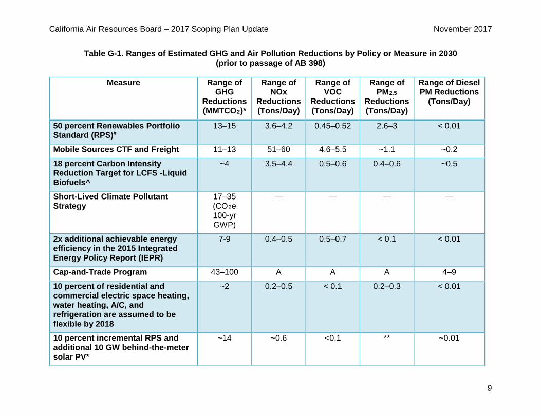
Section 2 – Tables: Ranges of Estimated Greenhouse Gas (GHG) and Air Pollution Reductions in 2030 The estimates in the tables below assume a one-to-one relationship between changes in GHGs, criteria pollutants, and toxic air contaminant emissions, and it is unclear whether that is always the case. The values should not be considered estimates of absolute changes for other analytical purposes. The ranges are estimates that represent current assumptions of how programs may be implemented; actual impacts may vary depending on the design, implementation, and performance of the policies and measures. The table does not show interactions between measures, such as the relationship with increased transportation electrification and associated increase in energy demand for the electricity sector.
California Air Resources Board – 2017 Scoping Plan November 2017
8
This Page Intentionally Left Blank
California Air Resources Board – 2017 Scoping Plan Update November 2017
9
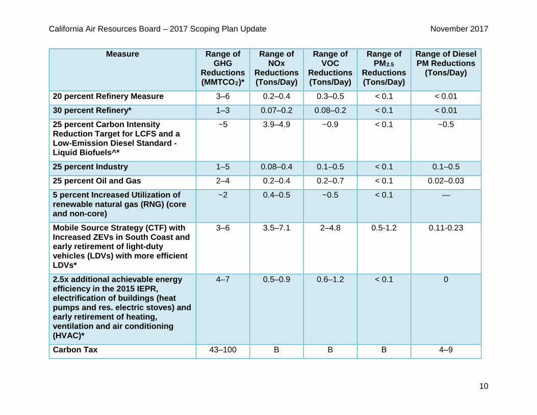
Table G-1. Ranges of Estimated GHG and Air Pollution Reductions by Policy or Measure in 2030 (prior to passage of AB 398)
Measure Range of
GHG Reductions (MMTCO2)*
Range of NOx
Reductions (Tons/Day)
Range of VOC
Reductions (Tons/Day)
Range of PM2.5
Reductions (Tons/Day)
Range of Diesel PM Reductions
(Tons/Day)
50 percent Renewables Portfolio Standard (RPS)#
13–15 3.6–4.2 0.45–0.52 2.6–3 < 0.01
Mobile Sources CTF and Freight 11–13 51–60 4.6–5.5 ~1.1 ~0.2
18 percent Carbon Intensity Reduction Target for LCFS -Liquid Biofuels^
~4 3.5–4.4 0.5–0.6 0.4–0.6 ~0.5
Short-Lived Climate Pollutant Strategy
17–35 (CO2e 100-yr GWP)
— — — —
2x additional achievable energy efficiency in the 2015 Integrated Energy Policy Report (IEPR)
7-9 0.4–0.5 0.5–0.7 < 0.1 < 0.01
Cap-and-Trade Program 43–100 A A A 4–9
10 percent of residential and commercial electric space heating, water heating, A/C, and refrigeration are assumed to be flexible by 2018
~2 0.2–0.5 < 0.1 0.2–0.3 < 0.01
10 percent incremental RPS and additional 10 GW behind-the-meter solar PV*
~14 ~0.6 <0.1 ** ~0.01
California Air Resources Board – 2017 Scoping Plan Update November 2017
10
Measure Range of GHG
Reductions (MMTCO2)*
Range of NOx
Reductions (Tons/Day)
Range of VOC
Reductions (Tons/Day)
Range of PM2.5
Reductions (Tons/Day)
Range of Diesel PM Reductions
(Tons/Day)
20 percent Refinery Measure 3–6 0.2–0.4 0.3–0.5 < 0.1 < 0.01
30 percent Refinery* 1–3 0.07–0.2 0.08–0.2 < 0.1 < 0.01
25 percent Carbon Intensity Reduction Target for LCFS and a Low-Emission Diesel Standard - Liquid Biofuels^*
~5 3.9–4.9 ~0.9 < 0.1 ~0.5
25 percent Industry 1–5 0.08–0.4 0.1–0.5 < 0.1 0.1–0.5
25 percent Oil and Gas 2–4 0.2–0.4 0.2–0.7 < 0.1 0.02–0.03
5 percent Increased Utilization of renewable natural gas (RNG) (core and non-core)
~2 0.4–0.5 ~0.5 < 0.1 —
Mobile Source Strategy (CTF) with Increased ZEVs in South Coast and early retirement of light-duty vehicles (LDVs) with more efficient LDVs*
3–6 3.5–7.1 2–4.8 0.5-1.2 0.11-0.23
2.5x additional achievable energy efficiency in the 2015 IEPR, electrification of buildings (heat pumps and res. electric stoves) and early retirement of heating, ventilation and air conditioning (HVAC)*
4–7 0.5–0.9 0.6–1.2 < 0.1 0
Carbon Tax 43–100 B B B 4–9
California Air Resources Board – 2017 Scoping Plan Update November 2017
11
Measure Range of GHG
Reductions (MMTCO2)*
Range of NOx
Reductions (Tons/Day)
Range of VOC
Reductions (Tons/Day)
Range of PM2.5
Reductions (Tons/Day)
Range of Diesel PM Reductions
(Tons/Day)
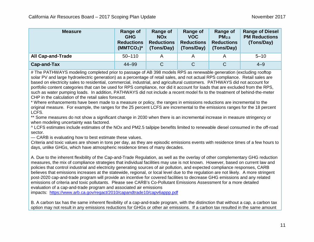
All Cap-and-Trade 50–110 A A A 5–10
Cap-and-Tax 44–99 C C C 4–9 # The PATHWAYS modeling completed prior to passage of AB 398 models RPS as renewable generation (excluding rooftop solar PV and large hydroelectric generation) as a percentage of retail sales, and not actual RPS compliance. Retail sales are based on electricity sales to residential, commercial, industrial, and agricultural customers. PATHWAYS did not account for portfolio content categories that can be used for RPS compliance, nor did it account for loads that are excluded from the RPS, such as water pumping loads. In addition, PATHWAYS did not include a recent model fix to the treatment of behind-the-meter CHP in the calculation of the retail sales forecast. * Where enhancements have been made to a measure or policy, the ranges in emissions reductions are incremental to the original measure. For example, the ranges for the 25 percent LCFS are incremental to the emissions ranges for the 18 percent LCFS. ** Some measures do not show a significant change in 2030 when there is an incremental increase in measure stringency or when modeling uncertainty was factored. ^ LCFS estimates include estimates of the NOx and PM2.5 tailpipe benefits limited to renewable diesel consumed in the off-road sector. — CARB is evaluating how to best estimate these values. Criteria and toxic values are shown in tons per day, as they are episodic emissions events with residence times of a few hours to days, unlike GHGs, which have atmospheric residence times of many decades. A. Due to the inherent flexibility of the Cap-and-Trade Regulation, as well as the overlay of other complementary GHG reduction measures, the mix of compliance strategies that individual facilities may use is not known. However, based on current law and policies that control industrial and electricity generating sources of air pollution, and expected compliance responses, CARB believes that emissions increases at the statewide, regional, or local level due to the regulation are not likely. A more stringent post-2020 cap-and-trade program will provide an incentive for covered facilities to decrease GHG emissions and any related emissions of criteria and toxic pollutants. Please see CARB’s Co-Pollutant Emissions Assessment for a more detailed evaluation of a cap-and-trade program and associated air emissions impacts: https://www.arb.ca.gov/regact/2010/capandtrade10/capv6appp.pdf B. A carbon tax has the same inherent flexibility of a cap-and-trade program, with the distinction that without a cap, a carbon tax option may not result in any emissions reductions for GHGs or other air emissions. If a carbon tax resulted in the same amount
California Air Resources Board – 2017 Scoping Plan Update November 2017
12
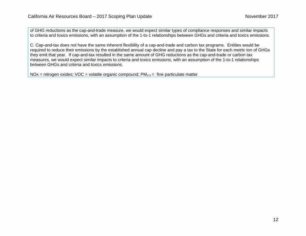
of GHG reductions as the cap-and-trade measure, we would expect similar types of compliance responses and similar impacts to criteria and toxics emissions, with an assumption of the 1-to-1 relationships between GHGs and criteria and toxics emissions. C. Cap-and-tax does not have the same inherent flexibility of a cap-and-trade and carbon tax programs. Entities would be required to reduce their emissions by the established annual cap decline and pay a tax to the State for each metric ton of GHGs they emit that year. If cap-and-tax resulted in the same amount of GHG reductions as the cap-and-trade or carbon tax measures, we would expect similar impacts to criteria and toxics emissions, with an assumption of the 1-to-1 relationships between GHGs and criteria and toxics emissions. NOx = nitrogen oxides; VOC = volatile organic compound; PM2.5 = fine particulate matter
California Air Resources Board – 2017 Scoping Plan Update November 2017
13
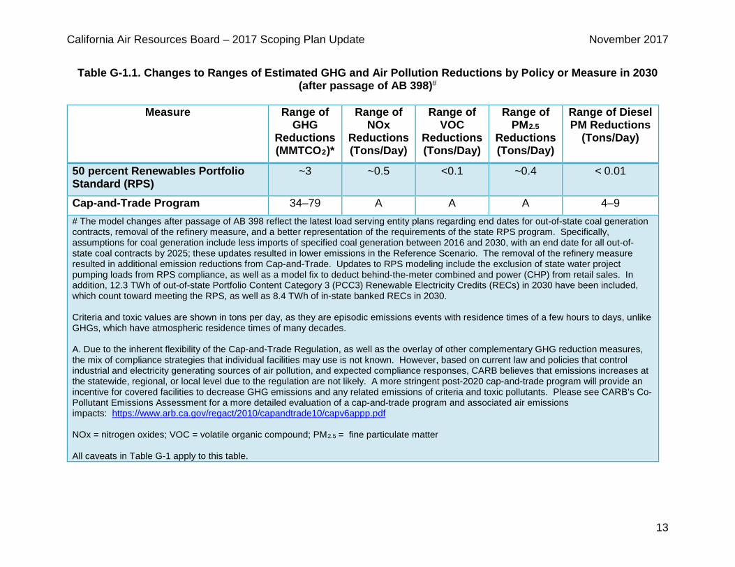
Table G-1.1. Changes to Ranges of Estimated GHG and Air Pollution Reductions by Policy or Measure in 2030 (after passage of AB 398)#
Measure Range of
GHG Reductions (MMTCO2)*
Range of NOx
Reductions (Tons/Day)
Range of VOC
Reductions (Tons/Day)
Range of PM2.5
Reductions (Tons/Day)
Range of Diesel PM Reductions
(Tons/Day)
50 percent Renewables Portfolio Standard (RPS)
~3 ~0.5 <0.1 ~0.4 < 0.01
Cap-and-Trade Program 34–79 A A A 4–9 # The model changes after passage of AB 398 reflect the latest load serving entity plans regarding end dates for out-of-state coal generation contracts, removal of the refinery measure, and a better representation of the requirements of the state RPS program. Specifically, assumptions for coal generation include less imports of specified coal generation between 2016 and 2030, with an end date for all out-of-state coal contracts by 2025; these updates resulted in lower emissions in the Reference Scenario. The removal of the refinery measure resulted in additional emission reductions from Cap-and-Trade. Updates to RPS modeling include the exclusion of state water project pumping loads from RPS compliance, as well as a model fix to deduct behind-the-meter combined and power (CHP) from retail sales. In addition, 12.3 TWh of out-of-state Portfolio Content Category 3 (PCC3) Renewable Electricity Credits (RECs) in 2030 have been included, which count toward meeting the RPS, as well as 8.4 TWh of in-state banked RECs in 2030.
Criteria and toxic values are shown in tons per day, as they are episodic emissions events with residence times of a few hours to days, unlike GHGs, which have atmospheric residence times of many decades. A. Due to the inherent flexibility of the Cap-and-Trade Regulation, as well as the overlay of other complementary GHG reduction measures, the mix of compliance strategies that individual facilities may use is not known. However, based on current law and policies that control industrial and electricity generating sources of air pollution, and expected compliance responses, CARB believes that emissions increases at the statewide, regional, or local level due to the regulation are not likely. A more stringent post-2020 cap-and-trade program will provide an incentive for covered facilities to decrease GHG emissions and any related emissions of criteria and toxic pollutants. Please see CARB’s Co-Pollutant Emissions Assessment for a more detailed evaluation of a cap-and-trade program and associated air emissions impacts: https://www.arb.ca.gov/regact/2010/capandtrade10/capv6appp.pdf NOx = nitrogen oxides; VOC = volatile organic compound; PM2.5 = fine particulate matter All caveats in Table G-1 apply to this table.
California Air Resources Board – 2017 Scoping Plan Update November 2017
14
This Page Intentionally Left Blank
California Air Resources Board – 2017 Scoping Plan Update November 2017
15
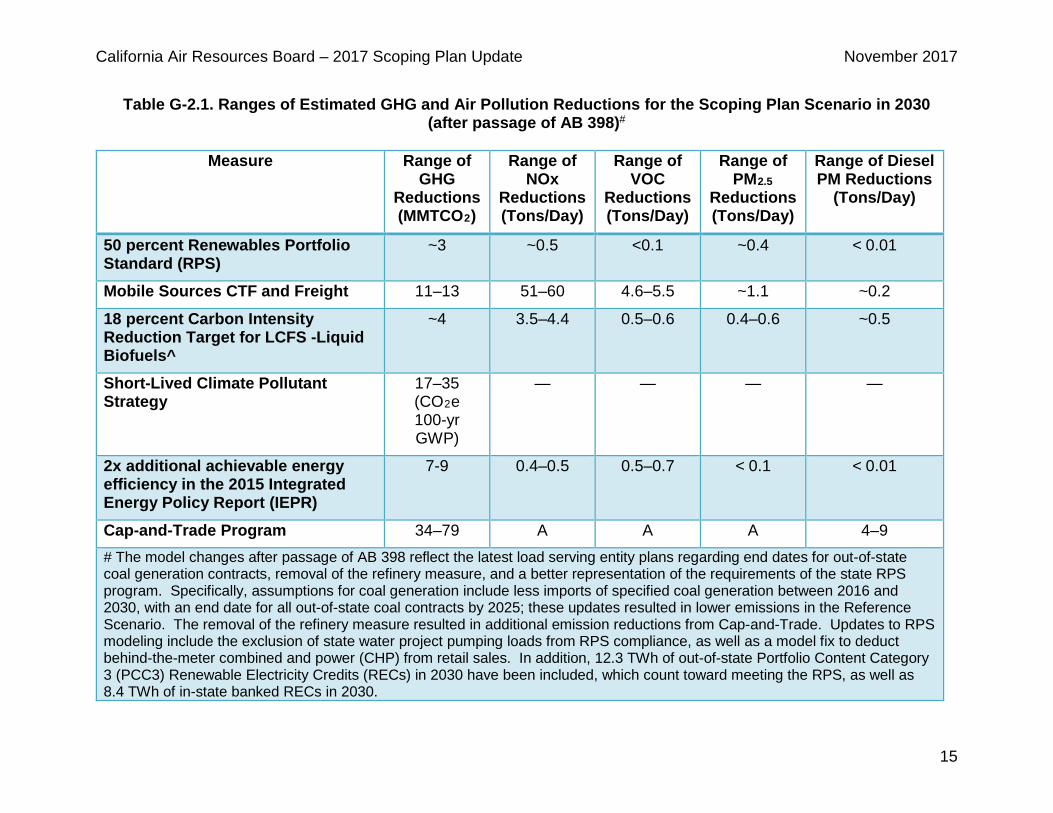
Table G-2.1. Ranges of Estimated GHG and Air Pollution Reductions for the Scoping Plan Scenario in 2030 (after passage of AB 398)#
Measure Range of
GHG Reductions (MMTCO2)
Range of NOx
Reductions (Tons/Day)
Range of VOC
Reductions (Tons/Day)
Range of PM2.5
Reductions (Tons/Day)
Range of Diesel PM Reductions
(Tons/Day)
50 percent Renewables Portfolio Standard (RPS)
~3 ~0.5 <0.1 ~0.4 < 0.01
Mobile Sources CTF and Freight 11–13 51–60 4.6–5.5 ~1.1 ~0.2
18 percent Carbon Intensity Reduction Target for LCFS -Liquid Biofuels^
~4 3.5–4.4 0.5–0.6 0.4–0.6 ~0.5
Short-Lived Climate Pollutant Strategy
17–35 (CO2e 100-yr GWP)
— — — —
2x additional achievable energy efficiency in the 2015 Integrated Energy Policy Report (IEPR)
7-9 0.4–0.5 0.5–0.7 < 0.1 < 0.01
Cap-and-Trade Program 34–79 A A A 4–9 # The model changes after passage of AB 398 reflect the latest load serving entity plans regarding end dates for out-of-state coal generation contracts, removal of the refinery measure, and a better representation of the requirements of the state RPS program. Specifically, assumptions for coal generation include less imports of specified coal generation between 2016 and 2030, with an end date for all out-of-state coal contracts by 2025; these updates resulted in lower emissions in the Reference Scenario. The removal of the refinery measure resulted in additional emission reductions from Cap-and-Trade. Updates to RPS modeling include the exclusion of state water project pumping loads from RPS compliance, as well as a model fix to deduct behind-the-meter combined and power (CHP) from retail sales. In addition, 12.3 TWh of out-of-state Portfolio Content Category 3 (PCC3) Renewable Electricity Credits (RECs) in 2030 have been included, which count toward meeting the RPS, as well as 8.4 TWh of in-state banked RECs in 2030.
California Air Resources Board – 2017 Scoping Plan Update November 2017
16
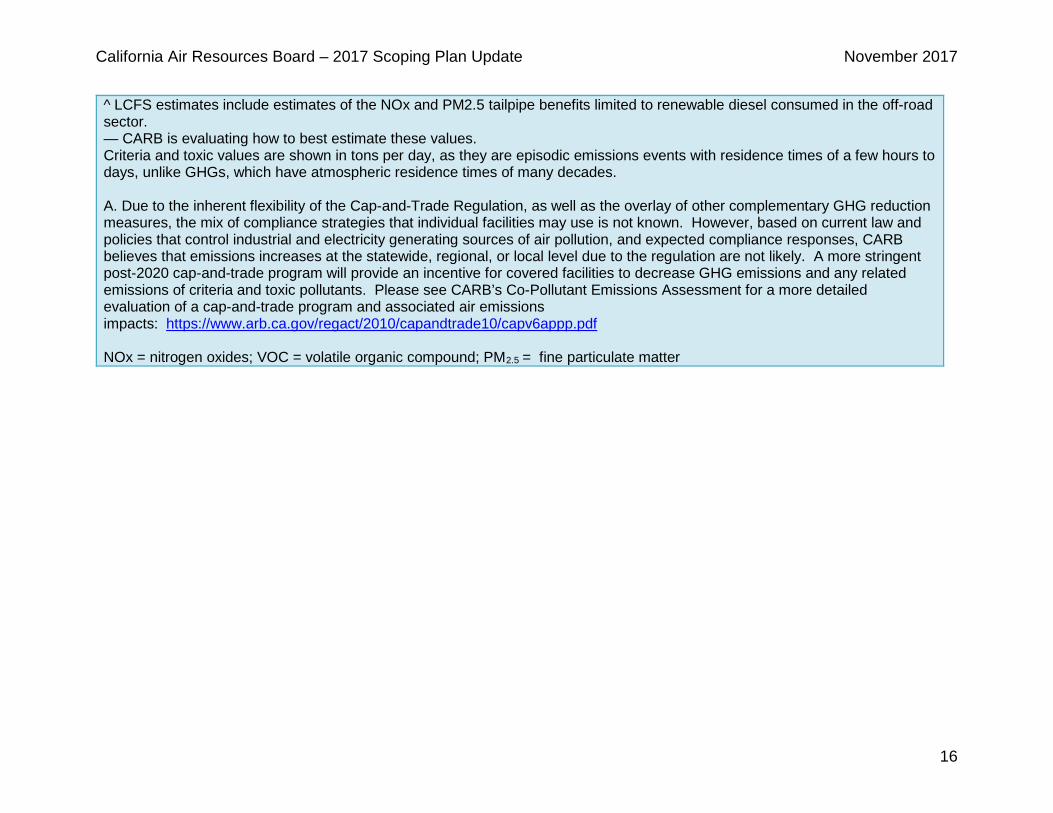
^ LCFS estimates include estimates of the NOx and PM2.5 tailpipe benefits limited to renewable diesel consumed in the off-road sector. — CARB is evaluating how to best estimate these values. Criteria and toxic values are shown in tons per day, as they are episodic emissions events with residence times of a few hours to days, unlike GHGs, which have atmospheric residence times of many decades. A. Due to the inherent flexibility of the Cap-and-Trade Regulation, as well as the overlay of other complementary GHG reduction measures, the mix of compliance strategies that individual facilities may use is not known. However, based on current law and policies that control industrial and electricity generating sources of air pollution, and expected compliance responses, CARB believes that emissions increases at the statewide, regional, or local level due to the regulation are not likely. A more stringent post-2020 cap-and-trade program will provide an incentive for covered facilities to decrease GHG emissions and any related emissions of criteria and toxic pollutants. Please see CARB’s Co-Pollutant Emissions Assessment for a more detailed evaluation of a cap-and-trade program and associated air emissions impacts: https://www.arb.ca.gov/regact/2010/capandtrade10/capv6appp.pdf NOx = nitrogen oxides; VOC = volatile organic compound; PM2.5 = fine particulate matter
California Air Resources Board – 2017 Scoping Plan Update November 2017
17
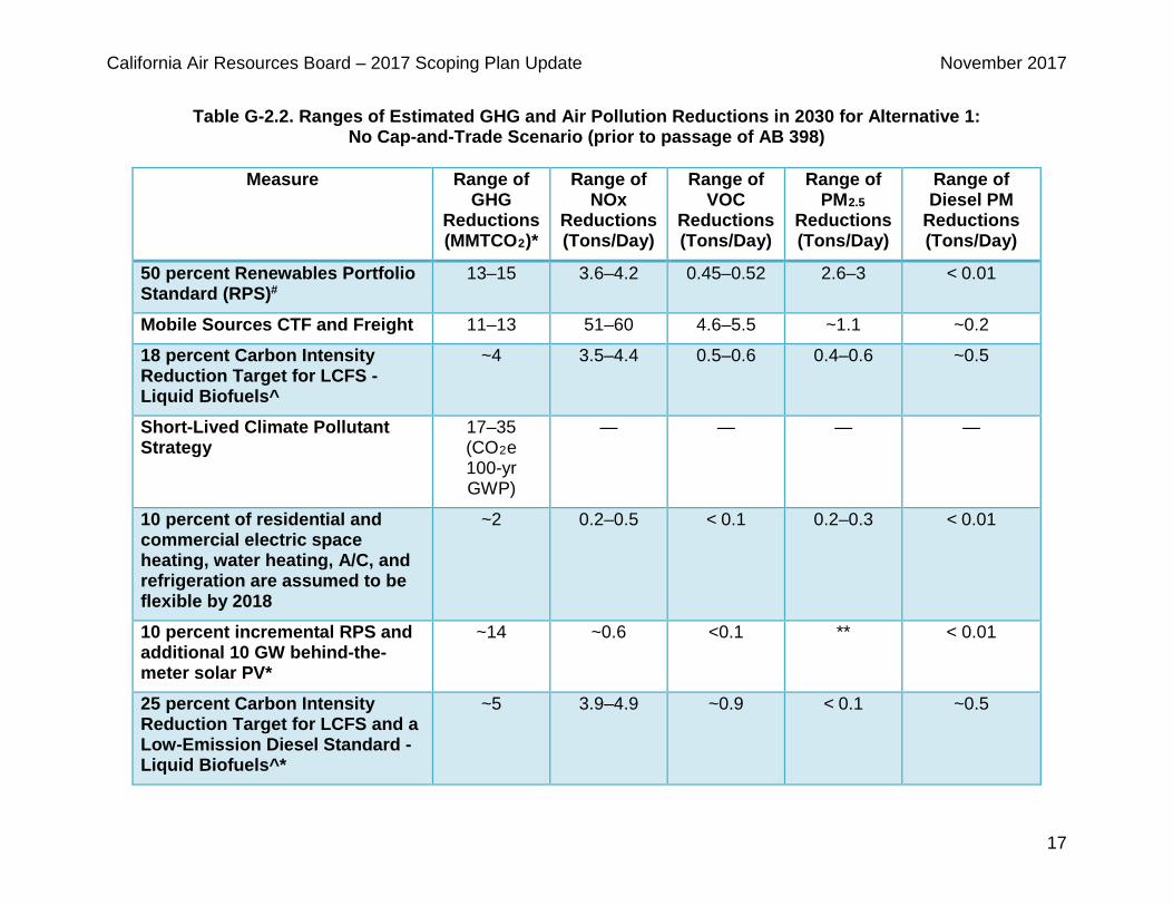
Table G-2.2. Ranges of Estimated GHG and Air Pollution Reductions in 2030 for Alternative 1: No Cap-and-Trade Scenario (prior to passage of AB 398)
Measure Range of
GHG Reductions (MMTCO2)*
Range of NOx
Reductions (Tons/Day)
Range of VOC
Reductions (Tons/Day)
Range of PM2.5
Reductions (Tons/Day)
Range of Diesel PM
Reductions (Tons/Day)
50 percent Renewables Portfolio Standard (RPS)#
13–15 3.6–4.2 0.45–0.52 2.6–3 < 0.01
Mobile Sources CTF and Freight 11–13 51–60 4.6–5.5 ~1.1 ~0.2
18 percent Carbon Intensity Reduction Target for LCFS -Liquid Biofuels^
~4 3.5–4.4 0.5–0.6 0.4–0.6 ~0.5
Short-Lived Climate Pollutant Strategy
17–35 (CO2e 100-yr GWP)
— — — —
10 percent of residential and commercial electric space heating, water heating, A/C, and refrigeration are assumed to be flexible by 2018
~2 0.2–0.5 < 0.1 0.2–0.3 < 0.01
10 percent incremental RPS and additional 10 GW behind-the-meter solar PV*
~14 ~0.6 <0.1 ** < 0.01
25 percent Carbon Intensity Reduction Target for LCFS and a Low-Emission Diesel Standard - Liquid Biofuels^*
~5 3.9–4.9 ~0.9 < 0.1 ~0.5
California Air Resources Board – 2017 Scoping Plan Update November 2017
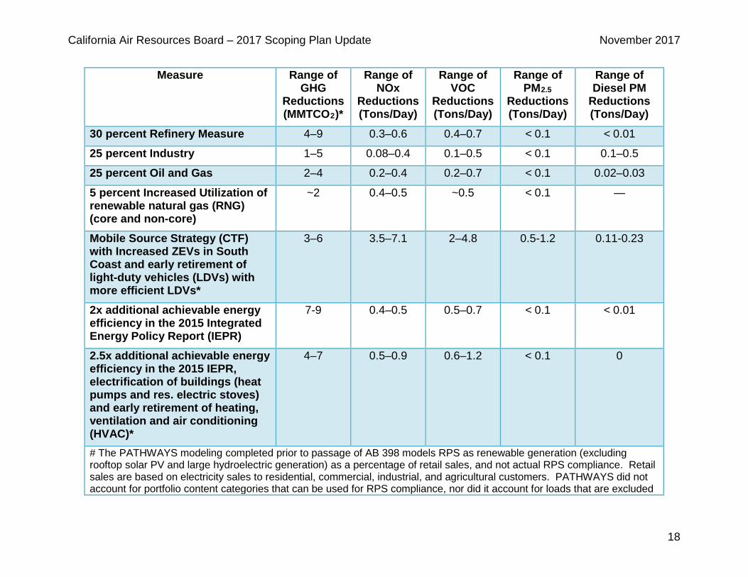
18
Measure Range of GHG
Reductions (MMTCO2)*
Range of NOx
Reductions (Tons/Day)
Range of VOC
Reductions (Tons/Day)
Range of PM2.5
Reductions (Tons/Day)
Range of Diesel PM
Reductions (Tons/Day)
30 percent Refinery Measure 4–9 0.3–0.6 0.4–0.7 < 0.1 < 0.01
25 percent Industry 1–5 0.08–0.4 0.1–0.5 < 0.1 0.1–0.5
25 percent Oil and Gas 2–4 0.2–0.4 0.2–0.7 < 0.1 0.02–0.03
5 percent Increased Utilization of renewable natural gas (RNG) (core and non-core)
~2 0.4–0.5 ~0.5 < 0.1 —
Mobile Source Strategy (CTF) with Increased ZEVs in South Coast and early retirement of light-duty vehicles (LDVs) with more efficient LDVs*
3–6 3.5–7.1 2–4.8 0.5-1.2 0.11-0.23
2x additional achievable energy efficiency in the 2015 Integrated Energy Policy Report (IEPR)
7-9 0.4–0.5 0.5–0.7 < 0.1 < 0.01
2.5x additional achievable energy efficiency in the 2015 IEPR, electrification of buildings (heat pumps and res. electric stoves) and early retirement of heating, ventilation and air conditioning (HVAC)*
4–7 0.5–0.9 0.6–1.2 < 0.1 0
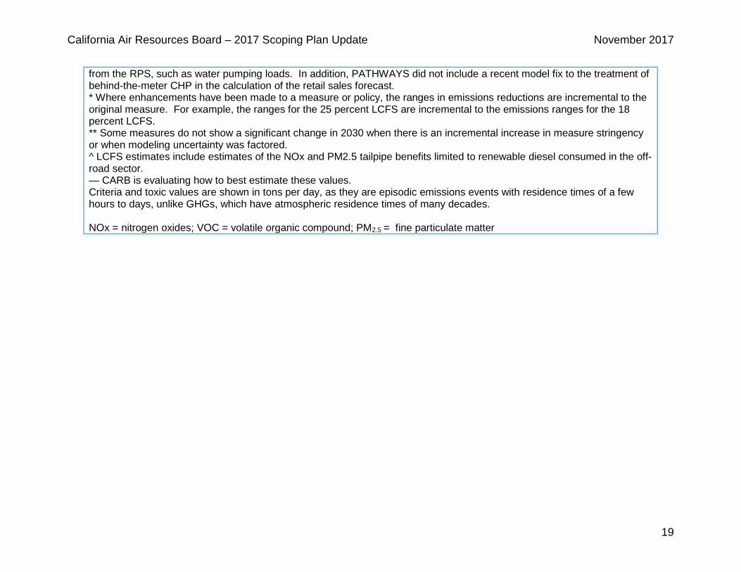
# The PATHWAYS modeling completed prior to passage of AB 398 models RPS as renewable generation (excluding rooftop solar PV and large hydroelectric generation) as a percentage of retail sales, and not actual RPS compliance. Retail sales are based on electricity sales to residential, commercial, industrial, and agricultural customers. PATHWAYS did not account for portfolio content categories that can be used for RPS compliance, nor did it account for loads that are excluded
California Air Resources Board – 2017 Scoping Plan Update November 2017
19
from the RPS, such as water pumping loads. In addition, PATHWAYS did not include a recent model fix to the treatment of behind-the-meter CHP in the calculation of the retail sales forecast. * Where enhancements have been made to a measure or policy, the ranges in emissions reductions are incremental to the original measure. For example, the ranges for the 25 percent LCFS are incremental to the emissions ranges for the 18 percent LCFS. ** Some measures do not show a significant change in 2030 when there is an incremental increase in measure stringency or when modeling uncertainty was factored. ^ LCFS estimates include estimates of the NOx and PM2.5 tailpipe benefits limited to renewable diesel consumed in the off-road sector. — CARB is evaluating how to best estimate these values. Criteria and toxic values are shown in tons per day, as they are episodic emissions events with residence times of a few hours to days, unlike GHGs, which have atmospheric residence times of many decades. NOx = nitrogen oxides; VOC = volatile organic compound; PM2.5 = fine particulate matter

California Air Resources Board – 2017 Scoping Plan Update November 2017
20
This Page Intentionally Left Blank
California Air Resources Board – 2017 Scoping Plan Update November 2017
21
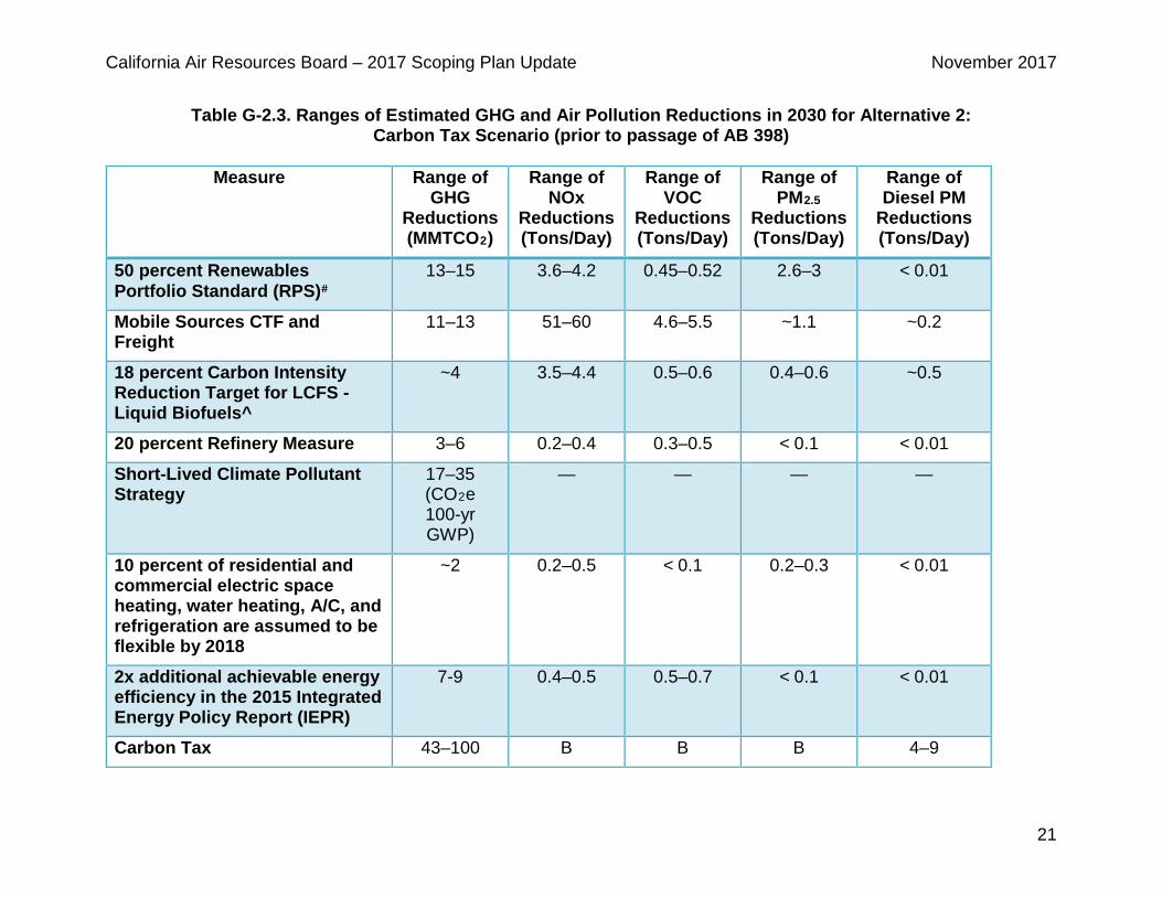
Table G-2.3. Ranges of Estimated GHG and Air Pollution Reductions in 2030 for Alternative 2: Carbon Tax Scenario (prior to passage of AB 398)
Measure Range of
GHG Reductions (MMTCO2)
Range of NOx
Reductions (Tons/Day)
Range of VOC
Reductions (Tons/Day)
Range of PM2.5
Reductions (Tons/Day)
Range of Diesel PM
Reductions (Tons/Day)
50 percent Renewables Portfolio Standard (RPS)#
13–15 3.6–4.2 0.45–0.52 2.6–3 < 0.01
Mobile Sources CTF and Freight
11–13 51–60 4.6–5.5 ~1.1 ~0.2
18 percent Carbon Intensity Reduction Target for LCFS -Liquid Biofuels^
~4 3.5–4.4 0.5–0.6 0.4–0.6 ~0.5
20 percent Refinery Measure 3–6 0.2–0.4 0.3–0.5 < 0.1 < 0.01
Short-Lived Climate Pollutant Strategy
17–35 (CO2e 100-yr GWP)
— — — —
10 percent of residential and commercial electric space heating, water heating, A/C, and refrigeration are assumed to be flexible by 2018
~2 0.2–0.5 < 0.1 0.2–0.3 < 0.01
2x additional achievable energy efficiency in the 2015 Integrated Energy Policy Report (IEPR)
7-9 0.4–0.5 0.5–0.7 < 0.1 < 0.01
Carbon Tax 43–100 B B B 4–9
California Air Resources Board – 2017 Scoping Plan Update November 2017
22
# The PATHWAYS modeling completed prior to passage of AB 398 models RPS as renewable generation (excluding rooftop solar PV and large hydroelectric generation) as a percentage of retail sales, and not actual RPS compliance. Retail sales are based on electricity sales to residential, commercial, industrial, and agricultural customers. PATHWAYS did not account for portfolio content categories that can be used for RPS compliance, nor did it account for loads that are excluded from the RPS, such as water pumping loads. In addition, PATHWAYS did not include a recent model fix to the treatment of behind-the-meter CHP in the calculation of the retail sales forecast. ^ LCFS estimates include estimates of the NOx and PM2.5 tailpipe benefits limited to renewable diesel consumed in the off-road sector. — CARB is evaluating how to best estimate these values. Criteria and toxic values are shown in tons per day, as they are episodic emissions events with residence times of a few hours to days, unlike GHGs, which have atmospheric residence times of many decades. B. A carbon tax has the same inherent flexibility of a cap-and-trade program, with the distinction that without a cap, a carbon tax option may not result in any emissions reductions for GHGs or other air emissions. If a carbon tax resulted in the same amount of GHG reductions as the cap-and-trade measure, we would expect similar types of compliance responses and similar impacts to criteria and toxics emissions, assuming the 1-to-1 relationships between GHGs and criteria and toxics emissions are real. NOx = nitrogen oxides; VOC = volatile organic compound; PM2.5 = fine particulate matter
California Air Resources Board – 2017 Scoping Plan Update November 2017
23
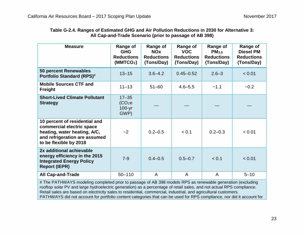
Table G-2.4. Ranges of Estimated GHG and Air Pollution Reductions in 2030 for Alternative 3: All Cap-and-Trade Scenario (prior to passage of AB 398)
Measure Range of
GHG Reductions (MMTCO2)
Range of NOx
Reductions (Tons/Day)
Range of VOC
Reductions (Tons/Day)
Range of PM2.5
Reductions (Tons/Day)
Range of Diesel PM
Reductions (Tons/Day)
50 percent Renewables Portfolio Standard (RPS)# 13–15 3.6–4.2 0.45–0.52 2.6–3 < 0.01
Mobile Sources CTF and Freight 11–13 51–60 4.6–5.5 ~1.1 ~0.2
Short-Lived Climate Pollutant Strategy
17–35 (CO2e 100-yr GWP)
— — — —
10 percent of residential and commercial electric space heating, water heating, A/C, and refrigeration are assumed to be flexible by 2018
~2 0.2–0.5 < 0.1 0.2–0.3 < 0.01
2x additional achievable energy efficiency in the 2015 Integrated Energy Policy Report (IEPR)
7-9 0.4–0.5 0.5–0.7 < 0.1 < 0.01
All Cap-and-Trade 50–110 A A A 5–10 # The PATHWAYS modeling completed prior to passage of AB 398 models RPS as renewable generation (excluding rooftop solar PV and large hydroelectric generation) as a percentage of retail sales, and not actual RPS compliance. Retail sales are based on electricity sales to residential, commercial, industrial, and agricultural customers. PATHWAYS did not account for portfolio content categories that can be used for RPS compliance, nor did it account for
California Air Resources Board – 2017 Scoping Plan Update November 2017
24
loads that are excluded from the RPS, such as water pumping loads. In addition, PATHWAYS did not include a recent model fix to the treatment of behind-the-meter CHP in the calculation of the retail sales forecast. — CARB is evaluating how to best estimate these values. Criteria and toxic values are shown in tons per day, as they are episodic emissions events with residence times of a few hours to days, unlike GHGs, which have atmospheric residence times of many decades. A. Due to the inherent flexibility of the Cap-and-Trade Regulation, as well as the overlay of other complementary GHG reduction measures, the mix of compliance strategies that individual facilities may use is not known. However, based on current law and policies that control industrial and electricity generating sources of air pollution, and expected compliance responses, CARB believes that emissions increases at the statewide, regional, or local level due to the regulation are not likely. A more stringent post-2020 cap-and-trade program will provide an incentive for covered facilities to decrease GHG emissions and any related emissions of criteria and toxic pollutants. Please see CARB’s Co-Pollutant Emissions Assessment for a more detailed evaluation of a cap-and-trade program and associated air emissions impacts: https://www.arb.ca.gov/regact/2010/capandtrade10/capv6appp.pdf NOx = nitrogen oxides; VOC = volatile organic compound; PM2.5 = fine particulate matter
California Air Resources Board – 2017 Scoping Plan Update November 2017
25
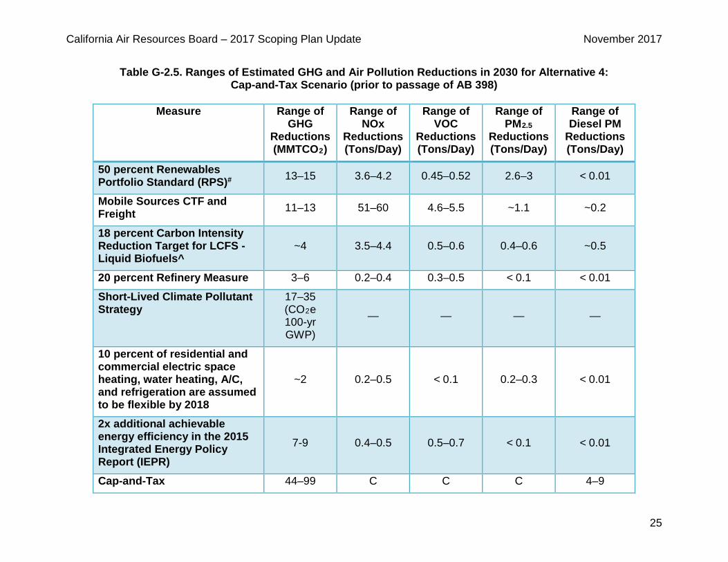
Table G-2.5. Ranges of Estimated GHG and Air Pollution Reductions in 2030 for Alternative 4: Cap-and-Tax Scenario (prior to passage of AB 398)
Measure
Range of GHG
Reductions (MMTCO2)
Range of NOx
Reductions (Tons/Day)
Range of VOC
Reductions (Tons/Day)
Range of PM2.5
Reductions (Tons/Day)
Range of Diesel PM
Reductions (Tons/Day)
50 percent Renewables Portfolio Standard (RPS)# 13–15 3.6–4.2 0.45–0.52 2.6–3 < 0.01
Mobile Sources CTF and Freight 11–13 51–60 4.6–5.5 ~1.1 ~0.2
18 percent Carbon Intensity Reduction Target for LCFS -Liquid Biofuels^
~4 3.5–4.4 0.5–0.6 0.4–0.6 ~0.5
20 percent Refinery Measure 3–6 0.2–0.4 0.3–0.5 < 0.1 < 0.01
Short-Lived Climate Pollutant Strategy
17–35 (CO2e 100-yr GWP)
— — — —
10 percent of residential and commercial electric space heating, water heating, A/C, and refrigeration are assumed to be flexible by 2018
~2 0.2–0.5 < 0.1 0.2–0.3 < 0.01
2x additional achievable energy efficiency in the 2015 Integrated Energy Policy Report (IEPR)
7-9 0.4–0.5 0.5–0.7 < 0.1 < 0.01
Cap-and-Tax 44–99 C C C 4–9
California Air Resources Board – 2017 Scoping Plan Update November 2017
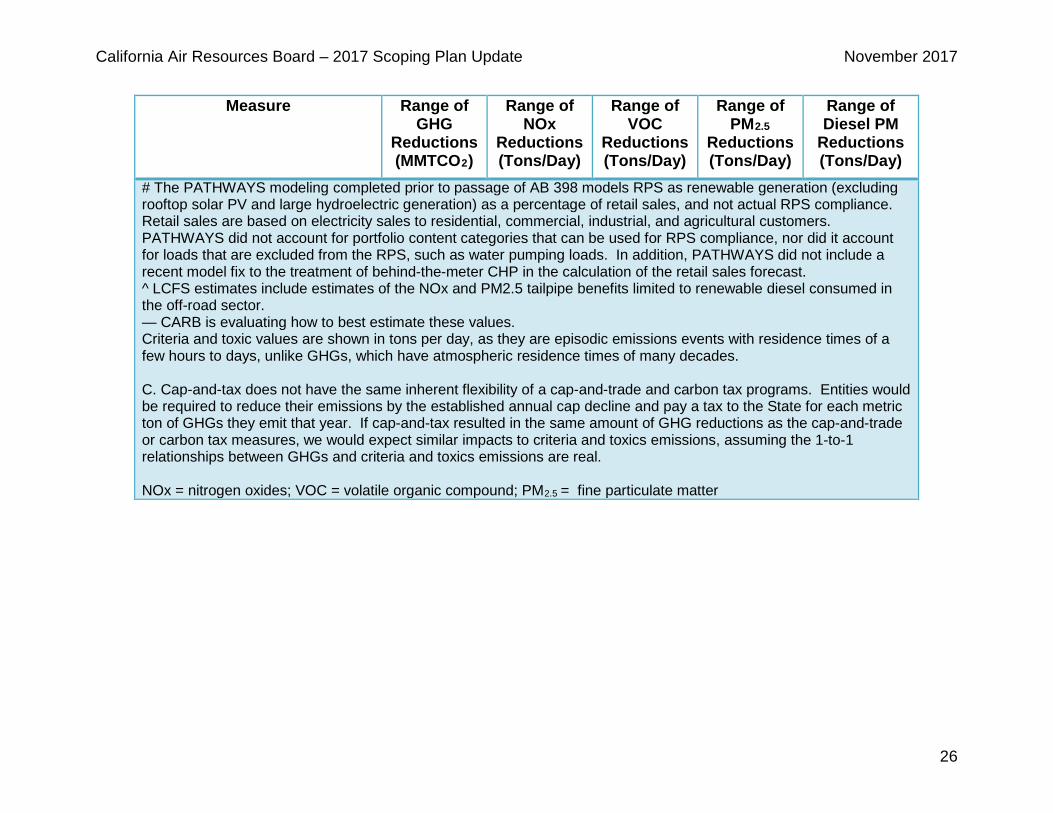
26
Measure
Range of GHG
Reductions (MMTCO2)
Range of NOx
Reductions (Tons/Day)
Range of VOC
Reductions (Tons/Day)
Range of PM2.5
Reductions (Tons/Day)
Range of Diesel PM
Reductions (Tons/Day)
# The PATHWAYS modeling completed prior to passage of AB 398 models RPS as renewable generation (excluding rooftop solar PV and large hydroelectric generation) as a percentage of retail sales, and not actual RPS compliance. Retail sales are based on electricity sales to residential, commercial, industrial, and agricultural customers. PATHWAYS did not account for portfolio content categories that can be used for RPS compliance, nor did it account for loads that are excluded from the RPS, such as water pumping loads. In addition, PATHWAYS did not include a recent model fix to the treatment of behind-the-meter CHP in the calculation of the retail sales forecast. ^ LCFS estimates include estimates of the NOx and PM2.5 tailpipe benefits limited to renewable diesel consumed in the off-road sector. — CARB is evaluating how to best estimate these values. Criteria and toxic values are shown in tons per day, as they are episodic emissions events with residence times of a few hours to days, unlike GHGs, which have atmospheric residence times of many decades. C. Cap-and-tax does not have the same inherent flexibility of a cap-and-trade and carbon tax programs. Entities would be required to reduce their emissions by the established annual cap decline and pay a tax to the State for each metric ton of GHGs they emit that year. If cap-and-tax resulted in the same amount of GHG reductions as the cap-and-trade or carbon tax measures, we would expect similar impacts to criteria and toxics emissions, assuming the 1-to-1 relationships between GHGs and criteria and toxics emissions are real. NOx = nitrogen oxides; VOC = volatile organic compound; PM2.5 = fine particulate matter
California Air Resources Board – 2017 Scoping Plan Update November 2017
27
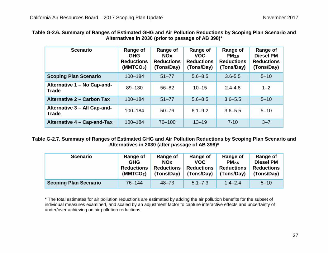
Table G-2.6. Summary of Ranges of Estimated GHG and Air Pollution Reductions by Scoping Plan Scenario and Alternatives in 2030 (prior to passage of AB 398)*
Scenario Range of
GHG Reductions (MMTCO2)
Range of NOx
Reductions (Tons/Day)
Range of VOC
Reductions (Tons/Day)
Range of PM2.5
Reductions (Tons/Day)
Range of Diesel PM
Reductions (Tons/Day)
Scoping Plan Scenario 100–184 51–77 5.6–8.5 3.6-5.5 5–10
Alternative 1 – No Cap-and-Trade 89–130 56–82 10–15 2.4-4.8 1–2
Alternative 2 – Carbon Tax 100–184 51–77 5.6–8.5 3.6–5.5 5–10
Alternative 3 – All Cap-and-Trade 100–184 50–76 6.1–9.2 3.6–5.5 5–10
Alternative 4 – Cap-and-Tax 100–184 70–100 13–19 7-10 3–7
Table G-2.7. Summary of Ranges of Estimated GHG and Air Pollution Reductions by Scoping Plan Scenario and
Alternatives in 2030 (after passage of AB 398)*
Scenario Range of GHG
Reductions (MMTCO2)
Range of NOx
Reductions (Tons/Day)
Range of VOC
Reductions (Tons/Day)
Range of PM2.5
Reductions (Tons/Day)
Range of Diesel PM
Reductions (Tons/Day)
Scoping Plan Scenario 76–144 48–73 5.1–7.3 1.4–2.4 5–10
* The total estimates for air pollution reductions are estimated by adding the air pollution benefits for the subset of individual measures examined, and scaled by an adjustment factor to capture interactive effects and uncertainty of under/over achieving on air pollution reductions.
California Air Resources Board – 2017 Scoping Plan Update November 2017
28
This Page Intentionally Left Blank
California Air Resources Board – 2017 Scoping Plan November 2017
29
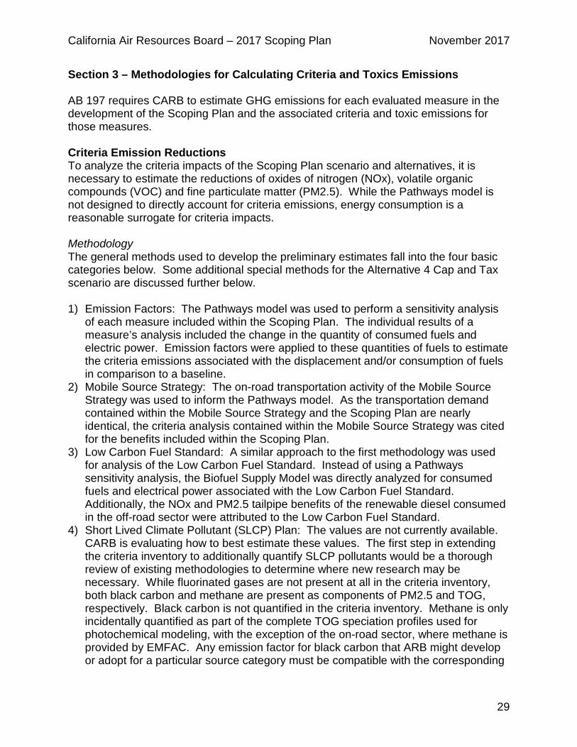
Section 3 – Methodologies for Calculating Criteria and Toxics Emissions AB 197 requires CARB to estimate GHG emissions for each evaluated measure in the development of the Scoping Plan and the associated criteria and toxic emissions for those measures. Criteria Emission Reductions To analyze the criteria impacts of the Scoping Plan scenario and alternatives, it is necessary to estimate the reductions of oxides of nitrogen (NOx), volatile organic compounds (VOC) and fine particulate matter (PM2.5). While the Pathways model is not designed to directly account for criteria emissions, energy consumption is a reasonable surrogate for criteria impacts. Methodology The general methods used to develop the preliminary estimates fall into the four basic categories below. Some additional special methods for the Alternative 4 Cap and Tax scenario are discussed further below. 1) Emission Factors: The Pathways model was used to perform a sensitivity analysis
of each measure included within the Scoping Plan. The individual results of a measure’s analysis included the change in the quantity of consumed fuels and electric power. Emission factors were applied to these quantities of fuels to estimate the criteria emissions associated with the displacement and/or consumption of fuels in comparison to a baseline.
2) Mobile Source Strategy: The on-road transportation activity of the Mobile Source Strategy was used to inform the Pathways model. As the transportation demand contained within the Mobile Source Strategy and the Scoping Plan are nearly identical, the criteria analysis contained within the Mobile Source Strategy was cited for the benefits included within the Scoping Plan.
3) Low Carbon Fuel Standard: A similar approach to the first methodology was used for analysis of the Low Carbon Fuel Standard. Instead of using a Pathways sensitivity analysis, the Biofuel Supply Model was directly analyzed for consumed fuels and electrical power associated with the Low Carbon Fuel Standard. Additionally, the NOx and PM2.5 tailpipe benefits of the renewable diesel consumed in the off-road sector were attributed to the Low Carbon Fuel Standard.
4) Short Lived Climate Pollutant (SLCP) Plan: The values are not currently available. CARB is evaluating how to best estimate these values. The first step in extending the criteria inventory to additionally quantify SLCP pollutants would be a thorough review of existing methodologies to determine where new research may be necessary. While fluorinated gases are not present at all in the criteria inventory, both black carbon and methane are present as components of PM2.5 and TOG, respectively. Black carbon is not quantified in the criteria inventory. Methane is only incidentally quantified as part of the complete TOG speciation profiles used for photochemical modeling, with the exception of the on-road sector, where methane is provided by EMFAC. Any emission factor for black carbon that ARB might develop or adopt for a particular source category must be compatible with the corresponding
California Air Resources Board – 2017 Scoping Plan November 2017
30
PM2.5 emission factor and applied to the same set of underlying activity data to ensure the emissions estimates that result are also compatible. Although methane can be estimated by applying TOG speciation profiles, that approach warrants additional review by staff because it is not an intended application of those profiles and may be less accurate than an approach using emission factors. New research will need to be performed to assess processes relevant to the SLCP plan that are currently not used in the criteria inventory, such as composting and land application of livestock wastes.
Method for Addressing Cap-and-Tax (Alternative 4) Scenario Methodology This section provides the analytic methodologies used, in lieu of modeling, to assess the change in energy demand and greenhouse gas (GHG) emissions associated with the modified Cap-and-Tax strategies. The Cap-and-Tax scenario adopts the Prescriptive Regulations (Alternative 1) assumptions and strategies, with some exceptions. Additional details of the modeling for this alternative are included in Appendix D. In order to ensure consistency with the other scenarios, the incremental reductions beyond the existing measures (as outlined in alternative 1) were summed into the Cap-and-Tax line item. The exceptions, and analytical methodologies used to quantify energy demand and GHG emissions are as follows: 1. Transportation: The transportation assumptions are identical to those in the
Prescriptive Regulations (Alternative 1) Scenario with the following exceptions: • 1 percent reduction in LDV VMT by 2030 – Quantified by reducing statewide
criteria emissions by 1 percent in 2030. • 10 percent rail electrification (passenger and freight) by 2050 – Quantified by
reducing rail criteria emissions by 3.3 percent in 2030 (assuming a linear interpolation between 0 percent in 2020 and 10 percent in 2050).
• The GHG benefits of Alternative 4 are the result of applying the NOx ratio, derived by dividing the Alternative 4 Transportation NOx emissions by the Alt 1 Transportation NOx emissions, to the Alt1 Transportation GHG emission benefits.
2. Building Energy Efficiency and Electrification: As a baseline, the same assumptions as the Prescriptive Regulations (Alternative 1) Scenario are used. Additional measures ensure that natural gas combustion in buildings achieves a 37 percent reduction in GHG emissions relative to 2020 Scoping Plan levels.
• Quantification of the natural gas efficiency in the residential and commercial building sector
A. Determined the 2020 Scoping Plan scenario’s residential and commercial building energy demand and applied a 37 percent reduction to the natural gas demand.
B. Criteria and GHG emission factors were applied to the reduced natural gas demand to quantify the air quality and GHG benefits.
• In lieu of modeling, a simplified approach to quantifying appliance electrification was used.
California Air Resources Board – 2017 Scoping Plan November 2017
31
A. The comparison of the Scoping Plan Scenario and the Prescriptive Regulations (Alternative 1) residential and commercial sector aggregate fuel demand indicated a 10 percent reduction in demand.
B. The comparison of the Scoping Plan Scenario and the Prescriptive Regulations (Alternative 1) residential and commercial sector electricity demand indicated a 7 percent reduction in demand.
C. This 3 percent difference is assumed to be the ratio of electrification in the residential and commercial building sector. This 3 percent was applied to the natural gas reductions due to efficiencies, and the resulting energy was assumed to be an increase in electricity demand.
3. Electricity Supply: As a baseline, the same assumptions as the Scoping Plan scenario are used. Additional renewable generation increases to 55 percent of retail sales by 2030.
• The electric power generation mix, on a pathway by pathway basis, was extrapolated from the Reference scenario’s 33 percent RPS and the Scoping Plan scenario’s 50 percent RPS to estimate the portfolio composition of a 55 percent RPS.
A. Per power generation pathway, criteria and GHG emission factors were applied to the power generation demands to quantify the air quality and GHG benefits.
4. Refining: As a baseline, the same assumptions as the Prescriptive Regulations (Alternative 1) Scenario are used. Additional measures achieve reductions in direct, on-site combustion emissions of 37 percent below 2020 Scoping Plan emissions levels in 2030.
• Quantification of the refining sector change in energy demand and emission benefits
A. Determined the 2020 Scoping Plan scenario’s refining sector’s energy demand and applied a standard 37 percent reduction to each energy pathway.
B. Criteria and GHG emission factors were applied to each pathway to quantify the air quality and GHG benefits.
5. Industrial (other manufacturing): As a baseline, the same assumptions as the Prescriptive Regulations (Alternative 1) Scenario are used. Additional measures achieve reductions in direct, on-site combustion emissions of 37 percent below 2020 Scoping Plan emissions levels in 2030.
• Quantification of the industrial sector change in energy demand and emission benefits
A. Determined the 2020 Scoping Plan scenario’s industrial sector’s energy demand and applied a standard 37 percent reduction to each energy pathway.
B. Criteria and GHG emission factors were applied to each pathway to quantify the air quality and GHG benefits.
6. Oil and Gas Extraction: As a baseline, the same assumptions as the Prescriptive Regulations (Alternative 1) Scenario are used. Additional measures achieve reductions in direct, on-site combustion emissions of 37 percent below 2020 Scoping Plan emissions levels in 2030.
California Air Resources Board – 2017 Scoping Plan November 2017
32
• Quantification of the oil and gas extraction sector change in energy demand and emission benefits
A. Determined the 2020 Scoping Plan scenario’s oil and gas extraction sector’s energy demand and applied a standard 37 percent reduction to each energy pathway.
B. Criteria and GHG emission factors were applied to each pathway to quantify the air quality and GHG benefits.
7. Non-Energy, Non-CO2 GHGs: As a baseline, the same assumptions as the Scoping Plan scenario are used. Additional measures meet the GHG caps assumed under the Cap-and-Tax Alternative. These include:
• Additional 17 percent reduction in manure methane A. Quantified by reducing GHG emissions associated with the agricultural
– manure sector in the Scoping Plan scenario by 17 percent. • Additional 20 percent reduction in waste emissions
A. Quantified by reducing GHG emissions associated with the waste sector in the Scoping Plan scenario by 20 percent.
• Additional 28 percent reduction in cement non-energy emissions A. Quantified by reducing GHG emissions associated with the cement
sector in the Scoping Plan scenario by 28 percent. The criteria emission factors used to quantify air quality impacts are standardized across all scenarios. The emission factors are applied, on a per energy pathway basis, to the avoided energy demand for individual strategies to estimate the criteria pollutant benefits. The GHG emission factors are derived by the Prescriptive Regulations (Alternative 1) scenario model outputs. On a per energy pathway basis, the aggregate GHG emissions for a unique pathway is divided by the energy demand for that unique pathway. This provides a MMTCO2E/EJ emission factor that is applied to the impacts of the Cap-and-Tax strategies to determine the GHG impacts. It is important to note that the criteria PM2.5 emission impacts are not always related directly with the diesel particulate matter. Most of the criteria PM2.5 analysis is focused on stationary and/or non-diesel sources, where the diesel particulate matter is almost entirely associated with mobile sources. Toxics Emission Reductions (Diesel PM) Toxic emissions are localized in their impacts, and without a full risk assessment for each release point, the relative risk (cancer, chronic and acute) of each toxic pollutant cannot be demonstrated at the statewide level. For purposes of this scoping plan analysis, staff chose to estimate instead a single pollutant -- the diesel particulate matter (DPM) associated with diesel engines. DPM accounts for a significant proportion of TAC health risks in the state, so emissions of DPM provide a useful indicator and comparative metric. Methodology The general methods used to develop the preliminary estimates fall into the basic categories below.
California Air Resources Board – 2017 Scoping Plan November 2017
33
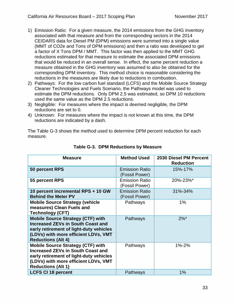
1) Emission Ratio: For a given measure, the 2014 emissions from the GHG inventory associated with that measure and from the corresponding sectors in the 2014 CEIDARS data for Diesel PM (DPM) emissions were summed into a single value (MMT of CO2e and Tons of DPM emissions) and then a ratio was developed to get a factor of X Tons DPM / MMT. This factor was then applied to the MMT GHG reductions estimated for that measure to estimate the associated DPM emissions that would be reduced in an overall sense. In effect, the same percent reduction a measure obtained in the GHG inventory was assumed to also be obtained for the corresponding DPM inventory. This method choice is reasonable considering the reductions in the measures are likely due to reductions in combustion.
2) Pathways: For the low carbon fuel standard (LCFS) and the Mobile Source Strategy Cleaner Technologies and Fuels Scenario, the Pathways model was used to estimate the DPM reductions. Only DPM 2.5 was estimated, so DPM 10 reductions used the same value as the DPM 2.5 reductions.
3) Negligible: For measures where the impact is deemed negligible, the DPM reductions are set to 0.
4) Unknown: For measures where the impact is not known at this time, the DPM reductions are indicated by a dash.
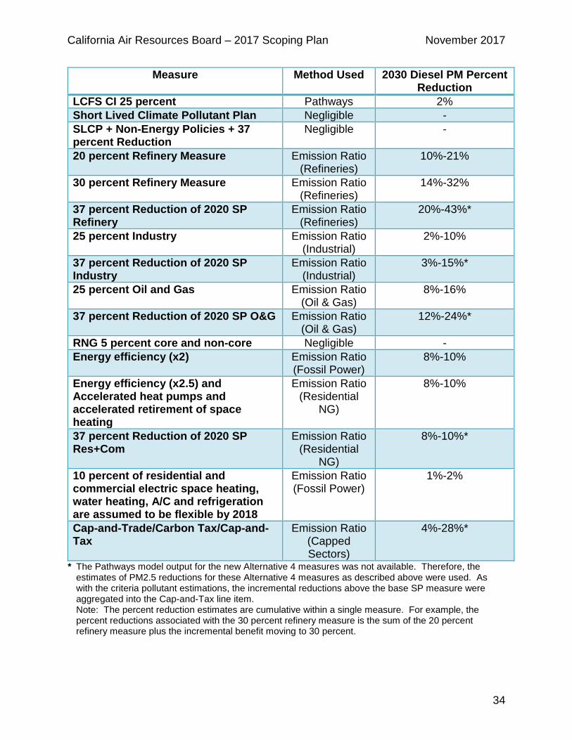
The Table G-3 shows the method used to determine DPM percent reduction for each measure.
Table G-3. DPM Reductions by Measure
Measure Method Used 2030 Diesel PM Percent Reduction
50 percent RPS Emission Ratio (Fossil Power)
15%-17%
55 percent RPS Emission Ratio (Fossil Power)
20%-23%*
10 percent incremental RPS + 10 GW Behind the Meter PV
Emission Ratio (Fossil Power)
31%-34%
Mobile Source Strategy (vehicle measures) Clean Fuels and Technology (CFT)
Pathways 1%
Mobile Source Strategy (CTF) with Increased ZEVs in South Coast and early retirement of light-duty vehicles (LDVs) with more efficient LDVs, VMT Reductions (Alt 4)
Pathways 2%*
Mobile Source Strategy (CTF) with Increased ZEVs in South Coast and early retirement of light-duty vehicles (LDVs) with more efficient LDVs, VMT Reductions (Alt 1)
Pathways 1%-2%
LCFS CI 18 percent Pathways 1%
California Air Resources Board – 2017 Scoping Plan November 2017
34
Measure Method Used 2030 Diesel PM Percent Reduction
LCFS CI 25 percent Pathways 2% Short Lived Climate Pollutant Plan Negligible - SLCP + Non-Energy Policies + 37 percent Reduction
Negligible -
20 percent Refinery Measure Emission Ratio (Refineries)
10%-21%
30 percent Refinery Measure Emission Ratio (Refineries)
14%-32%
37 percent Reduction of 2020 SP Refinery
Emission Ratio (Refineries)
20%-43%*
25 percent Industry Emission Ratio (Industrial)
2%-10%
37 percent Reduction of 2020 SP Industry
Emission Ratio (Industrial)
3%-15%*
25 percent Oil and Gas Emission Ratio (Oil & Gas)
8%-16%
37 percent Reduction of 2020 SP O&G Emission Ratio (Oil & Gas)
12%-24%*
RNG 5 percent core and non-core Negligible - Energy efficiency (x2) Emission Ratio
(Fossil Power) 8%-10%
Energy efficiency (x2.5) and Accelerated heat pumps and accelerated retirement of space heating
Emission Ratio (Residential
NG)
8%-10%
37 percent Reduction of 2020 SP Res+Com
Emission Ratio (Residential
NG)
8%-10%*
10 percent of residential and commercial electric space heating, water heating, A/C and refrigeration are assumed to be flexible by 2018
Emission Ratio (Fossil Power)
1%-2%
Cap-and-Trade/Carbon Tax/Cap-and-Tax
Emission Ratio (Capped Sectors)
4%-28%*
* The Pathways model output for the new Alternative 4 measures was not available. Therefore, the estimates of PM2.5 reductions for these Alternative 4 measures as described above were used. As with the criteria pollutant estimations, the incremental reductions above the base SP measure were aggregated into the Cap-and-Tax line item. Note: The percent reduction estimates are cumulative within a single measure. For example, the percent reductions associated with the 30 percent refinery measure is the sum of the 20 percent refinery measure plus the incremental benefit moving to 30 percent.
California Air Resources Board – 2017 Scoping Plan November 2017
35
Toxics estimation for the organic diversion of the SLCP No estimates for TACs are available at this time for the Short Lived Climate Pollutant plan. One of the reduction measures in SLCP involves diverting organic waste from landfills to other uses (composting, anaerobic digestion, etc.). Determining the air toxic contaminant impacts from this are complex and involve understanding the volatile organic compound and toxic speciation for landfilled organic waste and the diversion alternative. A lifecycle assessment for GHGs, criteria pollutants, and toxics emitted from the various management strategies for green waste, food waste, manure, and other biological material is necessary to answer these questions. Research is needed to understand each aspect of the lifecycle because the handling, transporting, processing, treatment, and utilization of biological material can affect each emissions species. For example, pile-turning frequency, type of feedstock, temperature, and moisture can affect composting emissions by orders of magnitude (this is also true for land application). CARB staff plans to work collaboratively with our sister agencies to further expand our understanding of this topic.
California Air Resources Board – 2017 Scoping Plan November 2017
36
This Page Intentionally Left Blank
California Air Resources Board – 2017 Scoping Plan November 2017
37
Section 4 – Health Risk Assessment and Quantifying Health Impacts Climate change will affect a variety of environmental factors, some of which will result in direct impacts on human health, and others of which will indirectly lead to adverse health outcomes. This section provides a summary of the health risk assessment and the methodology used to determine health impacts. Public Health Benefits of Climate Change Mitigation Warming temperatures, in the form of higher daily temperatures and longer and more frequent heatwaves, as well as higher overnight temperatures (and thus less night-time cooling) will be one consequence of a changing climate. Research published as part of the Second California Climate Assessment (Franco et al. 2011) showed that the association between elevated temperatures and human mortality is independent of air pollution (Basu et al., 2008) and that high temperatures have important morbidity effects measured by hospital admission data (Green et al., 2010). Additionally, urban areas tend to be warmer than surrounding regions; this is known as the “heat island effect.” This could result in exacerbated health impacts in large cities. In addition to heat-related deaths, heat exposure could lead to increases in heat stroke, dehydration, and worsened symptoms due to cardiovascular, respiratory, and cerebrovascular disease (EPA, https://www.epa.gov/climate-impacts/climate-impacts-human-health). Cayan et al. (2009) indicated that hot daytime and nighttime temperatures (heat waves) are increasing in frequency, magnitude, and duration from the historical period. Within a given heat wave, there is an increasing tendency for multiple hot days in succession, and the spatial footprint of heat waves is more and more likely to encompass multiple population centers in California. These findings heighten public health concerns in the coming decades. Furthermore, they showed that more days with conditions conducive to high tropospheric ozone levels will increase with climate change (Mahmud et al., 2008). This will result in an “air quality penalty” in the sense that more than the anticipated reduction of emissions of ozone precursors will have to be realized to be able to continue to improve air quality in California and eventually comply and maintain compliance with state and federal air quality standards. Health Benefits From PM2.5 Reductions California experiences some of the highest concentrations of PM2.5 in the nation (U.S. EPA, 2016). The majority of California’s population lives in areas that exceed the National Ambient Air Quality Standard for PM2.5 (ARB, 2015). This standard is set by the U.S. EPA, and is designed to protect human health and the environment from exposure to harmful levels of PM2.5. As part of the standard setting process, U.S. EPA assesses of scientific studies that link exposure to PM2.5 to health effects, including hospitalization due to respiratory illness, and premature death from cardiopulmonary disease (U.S. EPA, 2009). The U.S. EPA has determined that both long-term and short-term exposure to PM2.5 plays a “causal” role in premature death, meaning that a substantial body of scientific evidence shows a relationship between PM2.5 exposure and increased mortality, a relationship that persists when other risk factors such as
California Air Resources Board – 2017 Scoping Plan November 2017
38
smoking rates and socioeconomic factors are taken into account (U.S. EPA, 2009). These effects are also evidenced by a number of studies that have linked daily exposure to PM2.5 with hospitalization for heart and lung related causes, as well as an increase in emergency room visits, exacerbation of asthma, and other respiratory diseases (U.S. EPA, 2009). Methodology To estimate the health benefits from emission reductions in the Scoping Plan, the incidents-per-ton (IPT) methodology was used. This methodology is used to quantify the health benefits of directly emitted (primary) and secondary PM2.5 reductions due to regulatory controls. It is similar in concept to the methodology developed by the U.S. EPA for similar estimations (Fann et al., 2009), but uses California air basin specific relationships between emission and air quality. The basis of the IPT methodology is the approximately linear relationship which holds between changes in emissions and estimated changes in health outcomes. In this methodology, the number of premature deaths is estimated by multiplying emissions by a scaling factor, the IPT factor. The IPT factor is derived by calculating the number of incidents (premature deaths, hospitalizations, emergency room visits) associated with exposure to PM2.5 from a specific source, using concentration-response functions, described below, and dividing by the emissions of that PM2.5 source. The IPT factors used for primary PM2.5 in this assessment were originally developed for use with diesel PM emissions, but are also applied to PM from light-duty vehicles. This is justified on the grounds that emission patterns, dispersion mechanisms and loss mechanisms of primary PM from all on-road vehicular sources are expected to be similar. That is, a ton of PM emitted from on-road non-diesel vehicles is expected to result in the same PM2.5 exposure and health effects as a ton of PM emitted from on-road diesel trucks. IPT factors are calculated separately for each air basin by dividing the number of incidents in each air basin by primary PM emissions from that air basin. 𝐼𝐼𝐼𝐼𝐼𝐼 = number of incidents (deaths,hospitalizations,etc.) in air basin
𝑎𝑎𝑎𝑎𝑎𝑎𝑎𝑎𝑎𝑎𝑎𝑎 𝑒𝑒𝑒𝑒𝑒𝑒𝑒𝑒𝑒𝑒𝑒𝑒𝑒𝑒𝑎𝑎𝑒𝑒 𝑒𝑒𝑎𝑎 𝑎𝑎𝑒𝑒𝑎𝑎 𝑏𝑏𝑎𝑎𝑒𝑒𝑒𝑒𝑎𝑎 (𝑡𝑡𝑒𝑒𝑎𝑎𝑒𝑒/𝑦𝑦𝑒𝑒𝑎𝑎𝑎𝑎)
In addition to primary PM, motor vehicle exhaust contains NOx, a precursor to secondary ammonium nitrate PM that forms in the atmosphere. For secondary PM, the health impacts resulting from the three-year average exposure to ammonium nitrate PM was calculated and then associated the impacts with the basin-specific NOx emissions. Calculation of the change in premature death and other impacts associated with changes in PM2.5 exposure requires concentration-response functions (CRF), population data, baseline incidence rates, and the change in concentration of PM2.5 (ARB, 2010). Calculations are performed for each 2010 census tract and age bracket separately, then aggregated to totals by air basin. Five-year age brackets were used from ages 30 to 80, and an 85+ age bracket. Following recent U.S. EPA practice, CRF were used for premature mortality from Krewski et al. (2009), for hospital admissions from Bell et al. (2008), and for emergency room visits from Ito et al. (2007). For premature death, each CRF was assumed to be approximately linear down to a
California Air Resources Board – 2017 Scoping Plan November 2017
39
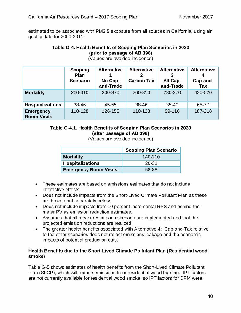
concentration of 5.8 μg/m3, the lowest concentration analyzed in Krewski et al. (2009), and reductions in PM2.5 to below that level were not quantified. Age-specific baseline incidence rates were taken from the CDC Wonder database. Population was estimated by taking 2010 Census data for total population by age bracket and projecting to 2030 using total county population projections from the California Department of Finance. This accounts for overall population growth in a county but does not reflect shifts in the spatial distribution of the population such as new housing developments built on previously undeveloped land. Emission reductions in the Scoping Plan come from a variety of air pollution sources. Sources at ground level in densely populated areas, such as motor vehicles in cities, will have a greater impact on the exposed population than sources emitted far above the ground or in sparsely populated areas. In order to account for the emission source variations, an intake fraction (IF) is used as a weighting factor. The IF is defined as the fraction of a source’s emissions that are inhaled by an exposed population. The application of the IF is described below for the Scoping Plan measures: Electric power: Electric power plants can be located far from cities and emit pollution from tall smokestacks, diluting their ground-level impacts for primary PM. Therefore, emissions for source categories where the bulk of the emissions are from electric power generation are multiplied by a weighting factor. Specifically, the weighting factor is the ratio of the IF for electrical power plants to the IF for on-road motor vehicles (e.g., passenger vehicles, heavy duty diesel trucks, etc.). Information regarding intake fraction of ground-level emissions and power plant emissions is derived from air pollution modeling studies. Marshall and Nazaroff (2004) calculated intake fraction values of primary pollutants such as PM from vehicular emissions for 17 major metropolitan statistical areas in California, ranging from 2.5 per million to 59 per million. Heath et al. (2006) calculated IF values of 25 existing central power plants for 13 counties in California, varying from 0.05 per million to 3.1 per million. The ratios of IFs for electric power plants over those for on-road motor vehicles range from 1/60 to 1/10, with an average of 1/30. The most health-protective value of 1/10 was used as the weighting factor for power plants. Other Industrial sectors: Other source categories such as petrochemical refineries also have elevated point releases, but IF data for these source categories currently are very limited, and more research is needed to fill this gap. Therefore, the health protective assumption was made that emissions from refineries is equally potent as emissions from on-road motor vehicles. A research study is currently being developed by ARB and collaborators to obtain better estimates of IFs for all major emission sectors/sources in California, including petrochemical refineries. Results Table G-4 shows the estimated reduction in mortality, hospitalizations, and emergency room visits associated with each Scoping Plan strategy. To put these estimates in context, 7,200 deaths, 1,900 hospitalizations, and 5,200 emergency room visits were
California Air Resources Board – 2017 Scoping Plan November 2017
40
estimated to be associated with PM2.5 exposure from all sources in California, using air quality data for 2009-2011.
Table G-4. Health Benefits of Scoping Plan Scenarios in 2030 (prior to passage of AB 398) (Values are avoided incidence)
Scoping
Plan Scenario
Alternative 1
No Cap-and-Trade
Alternative 2
Carbon Tax
Alternative 3
All Cap-and-Trade
Alternative 4
Cap-and-Tax
Mortality 260-310 300-370 260-310 230-270 430-520
Hospitalizations 38-46 45-55 38-46 35-40 65-77 Emergency Room Visits
110-128 126-155 110-128 99-116 187-218
Table G-4.1. Health Benefits of Scoping Plan Scenarios in 2030
(after passage of AB 398) (Values are avoided incidence)
Scoping Plan Scenario
Mortality 140-210 Hospitalizations 20-31 Emergency Room Visits 58-88
• These estimates are based on emissions estimates that do not include interactive effects.
• Does not include impacts from the Short-Lived Climate Pollutant Plan as these are broken out separately below.
• Does not include impacts from 10 percent incremental RPS and behind-the-meter PV as emission reduction estimates.
• Assumes that all measures in each scenario are implemented and that the projected emission reductions are realized.
• The greater health benefits associated with Alternative 4: Cap-and-Tax relative to the other scenarios does not reflect emissions leakage and the economic impacts of potential production cuts.
Health Benefits due to the Short-Lived Climate Pollutant Plan (Residential wood smoke) Table G-5 shows estimates of health benefits from the Short-Lived Climate Pollutant Plan (SLCP), which will reduce emissions from residential wood burning. IPT factors are not currently available for residential wood smoke, so IPT factors for DPM were
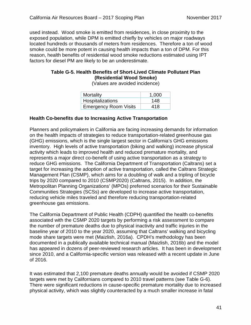
California Air Resources Board – 2017 Scoping Plan November 2017
41
used instead. Wood smoke is emitted from residences, in close proximity to the exposed population, while DPM is emitted chiefly by vehicles on major roadways located hundreds or thousands of meters from residences. Therefore a ton of wood smoke could be more potent in causing health impacts than a ton of DPM. For this reason, health benefits of residential wood smoke reductions estimated using IPT factors for diesel PM are likely to be an underestimate.
Table G-5. Health Benefits of Short-Lived Climate Pollutant Plan (Residential Wood Smoke)
(Values are avoided incidence)
Mortality 1,000 Hospitalizations 148 Emergency Room Visits 418
Health Co-benefits due to Increasing Active Transportation Planners and policymakers in California are facing increasing demands for information on the health impacts of strategies to reduce transportation-related greenhouse gas (GHG) emissions, which is the single largest sector in California’s GHG emissions inventory. High levels of active transportation (biking and walking) increase physical activity which leads to improved health and reduced premature mortality, and represents a major direct co-benefit of using active transportation as a strategy to reduce GHG emissions. The California Department of Transportation (Caltrans) set a target for increasing the adoption of active transportation, called the Caltrans Strategic Management Plan (CSMP), which aims for a doubling of walk and a tripling of bicycle trips by 2020 compared to 2010 (CSMP2020) (Caltrans, 2015). In addition, the Metropolitan Planning Organizations’ (MPOs) preferred scenarios for their Sustainable Communities Strategies (SCSs) are developed to increase active transportation, reducing vehicle miles traveled and therefore reducing transportation-related greenhouse gas emissions. The California Department of Public Health (CDPH) quantified the health co-benefits associated with the CSMP 2020 targets by performing a risk assessment to compare the number of premature deaths due to physical inactivity and traffic injuries in the baseline year of 2010 to the year 2020, assuming that Caltrans’ walking and bicycling mode share targets were met (Maizlish, 2016a). CPDH’s methodology has been documented in a publically available technical manual (Maizlish, 2016b) and the model has appeared in dozens of peer-reviewed research articles. It has been in development since 2010, and a California-specific version was released with a recent update in June of 2016. It was estimated that 2,100 premature deaths annually would be avoided if CSMP 2020 targets were met by Californians compared to 2010 travel patterns (see Table G-6). There were significant reductions in cause-specific premature mortality due to increased physical activity, which was slightly counteracted by a much smaller increase in fatal
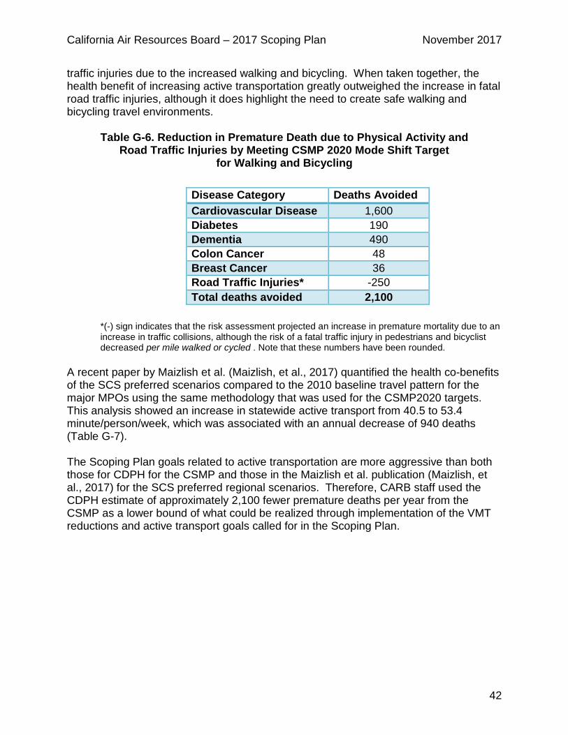
California Air Resources Board – 2017 Scoping Plan November 2017
42
traffic injuries due to the increased walking and bicycling. When taken together, the health benefit of increasing active transportation greatly outweighed the increase in fatal road traffic injuries, although it does highlight the need to create safe walking and bicycling travel environments.
Table G-6. Reduction in Premature Death due to Physical Activity and Road Traffic Injuries by Meeting CSMP 2020 Mode Shift Target
for Walking and Bicycling
*(-) sign indicates that the risk assessment projected an increase in premature mortality due to an increase in traffic collisions, although the risk of a fatal traffic injury in pedestrians and bicyclist decreased per mile walked or cycled . Note that these numbers have been rounded.
A recent paper by Maizlish et al. (Maizlish, et al., 2017) quantified the health co-benefits of the SCS preferred scenarios compared to the 2010 baseline travel pattern for the major MPOs using the same methodology that was used for the CSMP2020 targets. This analysis showed an increase in statewide active transport from 40.5 to 53.4 minute/person/week, which was associated with an annual decrease of 940 deaths (Table G-7). The Scoping Plan goals related to active transportation are more aggressive than both those for CDPH for the CSMP and those in the Maizlish et al. publication (Maizlish, et al., 2017) for the SCS preferred regional scenarios. Therefore, CARB staff used the CDPH estimate of approximately 2,100 fewer premature deaths per year from the CSMP as a lower bound of what could be realized through implementation of the VMT reductions and active transport goals called for in the Scoping Plan.
Disease Category Deaths Avoided Cardiovascular Disease 1,600 Diabetes 190 Dementia 490 Colon Cancer 48 Breast Cancer 36 Road Traffic Injuries* -250 Total deaths avoided 2,100
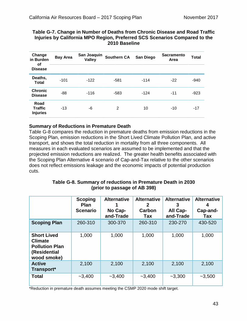
California Air Resources Board – 2017 Scoping Plan November 2017
43
Table G-7. Change in Number of Deaths from Chronic Disease and Road Traffic Injuries by California MPO Region, Preferred SCS Scenarios Compared to the
2010 Baseline
Change in Burden
of Disease
Bay Area San Joaquin Valley Southern CA San Diego Sacramento
Area Total
Deaths, Total -101 -122 -581 -114 -22 -940
Chronic Disease -88 -116 -583 -124 -11 -923
Road Traffic Injuries
-13 -6 2 10 -10 -17
Summary of Reductions in Premature Death Table G-8 compares the reduction in premature deaths from emission reductions in the Scoping Plan, emission reductions in the Short Lived Climate Pollution Plan, and active transport, and shows the total reduction in mortality from all three components. All measures in each evaluated scenarios are assumed to be implemented and that the projected emission reductions are realized. The greater health benefits associated with the Scoping Plan Alternative 4 scenario of Cap-and-Tax relative to the other scenarios does not reflect emissions leakage and the economic impacts of potential production cuts.
Table G-8. Summary of reductions in Premature Death in 2030 (prior to passage of AB 398)
Scoping
Plan Scenario
Alternative 1
No Cap-and-Trade
Alternative 2
Carbon Tax
Alternative 3
All Cap-and-Trade
Alternative 4
Cap-and-Tax
Scoping Plan 260-310 300-370 260-310 230-270 430-520
Short Lived Climate Pollution Plan (Residential wood smoke)
1,000 1,000 1,000 1,000 1,000
Active Transport*
2,100 2,100 2,100 2,100 2,100
Total ~3,400 ~3,400 ~3,400 ~3,300 ~3,500
*Reduction in premature death assumes meeting the CSMP 2020 mode shift target.
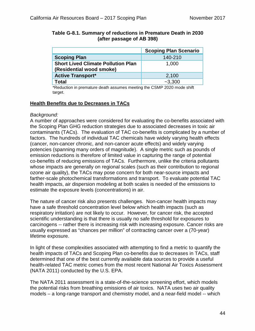
California Air Resources Board – 2017 Scoping Plan November 2017
44
Table G-8.1. Summary of reductions in Premature Death in 2030 (after passage of AB 398)
Scoping Plan Scenario
Scoping Plan 140-210 Short Lived Climate Pollution Plan (Residential wood smoke)
1,000
Active Transport* 2,100 Total ~3,300
*Reduction in premature death assumes meeting the CSMP 2020 mode shift target.
Health Benefits due to Decreases in TACs Background: A number of approaches were considered for evaluating the co-benefits associated with the Scoping Plan GHG reduction strategies due to associated decreases in toxic air contaminants (TACs). The evaluation of TAC co-benefits is complicated by a number of factors. The hundreds of individual TAC chemicals have widely varying health effects (cancer, non-cancer chronic, and non-cancer acute effects) and widely varying potencies (spanning many orders of magnitude). A single metric such as pounds of emission reductions is therefore of limited value in capturing the range of potential co-benefits of reducing emissions of TACs. Furthermore, unlike the criteria pollutants whose impacts are generally on regional scales (such as their contribution to regional ozone air quality), the TACs may pose concern for both near-source impacts and farther-scale photochemical transformations and transport. To evaluate potential TAC health impacts, air dispersion modeling at both scales is needed of the emissions to estimate the exposure levels (concentrations) in air. The nature of cancer risk also presents challenges. Non-cancer health impacts may have a safe threshold concentration level below which health impacts (such as respiratory irritation) are not likely to occur. However, for cancer risk, the accepted scientific understanding is that there is usually no safe threshold for exposures to carcinogens -- rather there is increasing risk with increasing exposure. Cancer risks are usually expressed as “chances per million” of contracting cancer over a (70-year) lifetime exposure. In light of these complexities associated with attempting to find a metric to quantify the health impacts of TACs and Scoping Plan co-benefits due to decreases in TACs, staff determined that one of the best currently available data sources to provide a useful health-related TAC metric comes from the most recent National Air Toxics Assessment (NATA 2011) conducted by the U.S. EPA. The NATA 2011 assessment is a state-of-the-science screening effort, which models the potential risks from breathing emissions of air toxics. NATA uses two air quality models – a long-range transport and chemistry model, and a near-field model -- which
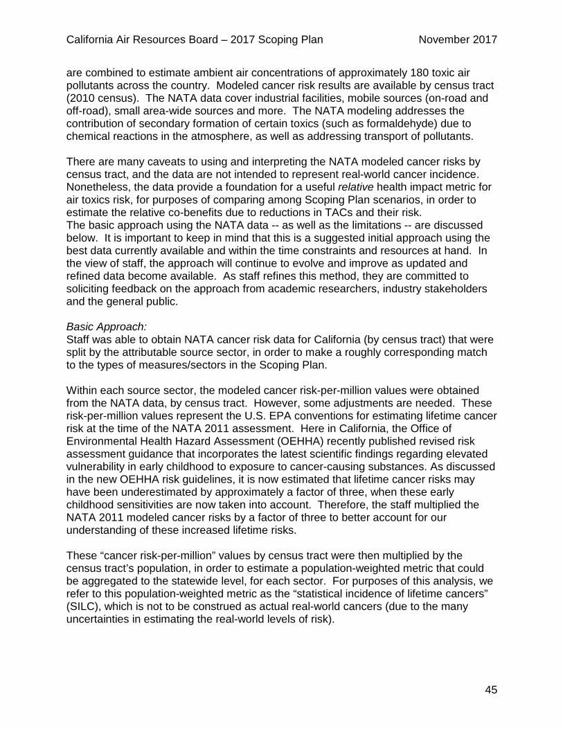
California Air Resources Board – 2017 Scoping Plan November 2017
45
are combined to estimate ambient air concentrations of approximately 180 toxic air pollutants across the country. Modeled cancer risk results are available by census tract (2010 census). The NATA data cover industrial facilities, mobile sources (on-road and off-road), small area-wide sources and more. The NATA modeling addresses the contribution of secondary formation of certain toxics (such as formaldehyde) due to chemical reactions in the atmosphere, as well as addressing transport of pollutants. There are many caveats to using and interpreting the NATA modeled cancer risks by census tract, and the data are not intended to represent real-world cancer incidence. Nonetheless, the data provide a foundation for a useful relative health impact metric for air toxics risk, for purposes of comparing among Scoping Plan scenarios, in order to estimate the relative co-benefits due to reductions in TACs and their risk. The basic approach using the NATA data -- as well as the limitations -- are discussed below. It is important to keep in mind that this is a suggested initial approach using the best data currently available and within the time constraints and resources at hand. In the view of staff, the approach will continue to evolve and improve as updated and refined data become available. As staff refines this method, they are committed to soliciting feedback on the approach from academic researchers, industry stakeholders and the general public. Basic Approach: Staff was able to obtain NATA cancer risk data for California (by census tract) that were split by the attributable source sector, in order to make a roughly corresponding match to the types of measures/sectors in the Scoping Plan. Within each source sector, the modeled cancer risk-per-million values were obtained from the NATA data, by census tract. However, some adjustments are needed. These risk-per-million values represent the U.S. EPA conventions for estimating lifetime cancer risk at the time of the NATA 2011 assessment. Here in California, the Office of Environmental Health Hazard Assessment (OEHHA) recently published revised risk assessment guidance that incorporates the latest scientific findings regarding elevated vulnerability in early childhood to exposure to cancer-causing substances. As discussed in the new OEHHA risk guidelines, it is now estimated that lifetime cancer risks may have been underestimated by approximately a factor of three, when these early childhood sensitivities are now taken into account. Therefore, the staff multiplied the NATA 2011 modeled cancer risks by a factor of three to better account for our understanding of these increased lifetime risks. These “cancer risk-per-million” values by census tract were then multiplied by the census tract’s population, in order to estimate a population-weighted metric that could be aggregated to the statewide level, for each sector. For purposes of this analysis, we refer to this population-weighted metric as the “statistical incidence of lifetime cancers” (SILC), which is not to be construed as actual real-world cancers (due to the many uncertainties in estimating the real-world levels of risk).
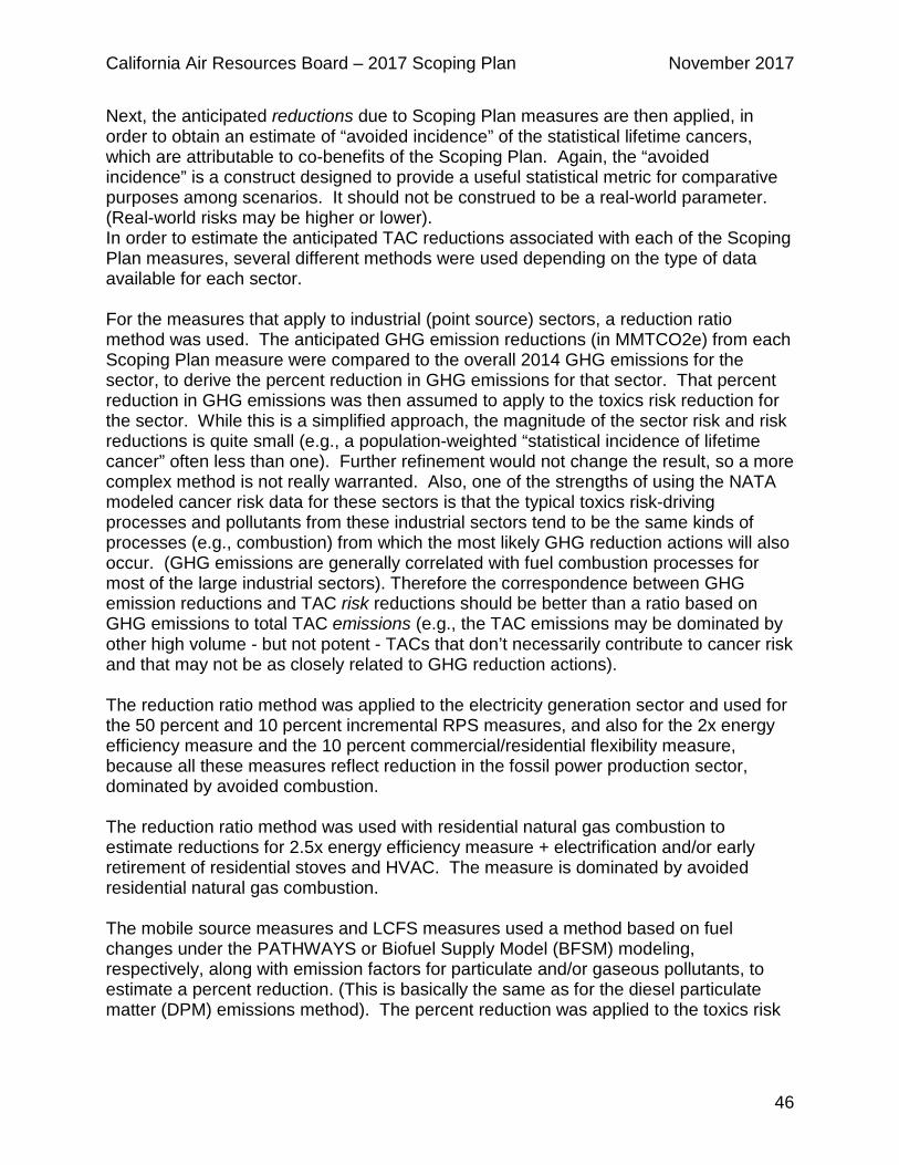
California Air Resources Board – 2017 Scoping Plan November 2017
46
Next, the anticipated reductions due to Scoping Plan measures are then applied, in order to obtain an estimate of “avoided incidence” of the statistical lifetime cancers, which are attributable to co-benefits of the Scoping Plan. Again, the “avoided incidence” is a construct designed to provide a useful statistical metric for comparative purposes among scenarios. It should not be construed to be a real-world parameter. (Real-world risks may be higher or lower). In order to estimate the anticipated TAC reductions associated with each of the Scoping Plan measures, several different methods were used depending on the type of data available for each sector. For the measures that apply to industrial (point source) sectors, a reduction ratio method was used. The anticipated GHG emission reductions (in MMTCO2e) from each Scoping Plan measure were compared to the overall 2014 GHG emissions for the sector, to derive the percent reduction in GHG emissions for that sector. That percent reduction in GHG emissions was then assumed to apply to the toxics risk reduction for the sector. While this is a simplified approach, the magnitude of the sector risk and risk reductions is quite small (e.g., a population-weighted “statistical incidence of lifetime cancer” often less than one). Further refinement would not change the result, so a more complex method is not really warranted. Also, one of the strengths of using the NATA modeled cancer risk data for these sectors is that the typical toxics risk-driving processes and pollutants from these industrial sectors tend to be the same kinds of processes (e.g., combustion) from which the most likely GHG reduction actions will also occur. (GHG emissions are generally correlated with fuel combustion processes for most of the large industrial sectors). Therefore the correspondence between GHG emission reductions and TAC risk reductions should be better than a ratio based on GHG emissions to total TAC emissions (e.g., the TAC emissions may be dominated by other high volume - but not potent - TACs that don’t necessarily contribute to cancer risk and that may not be as closely related to GHG reduction actions). The reduction ratio method was applied to the electricity generation sector and used for the 50 percent and 10 percent incremental RPS measures, and also for the 2x energy efficiency measure and the 10 percent commercial/residential flexibility measure, because all these measures reflect reduction in the fossil power production sector, dominated by avoided combustion. The reduction ratio method was used with residential natural gas combustion to estimate reductions for 2.5x energy efficiency measure + electrification and/or early retirement of residential stoves and HVAC. The measure is dominated by avoided residential natural gas combustion. The mobile source measures and LCFS measures used a method based on fuel changes under the PATHWAYS or Biofuel Supply Model (BFSM) modeling, respectively, along with emission factors for particulate and/or gaseous pollutants, to estimate a percent reduction. (This is basically the same as for the diesel particulate matter (DPM) emissions method). The percent reduction was applied to the toxics risk
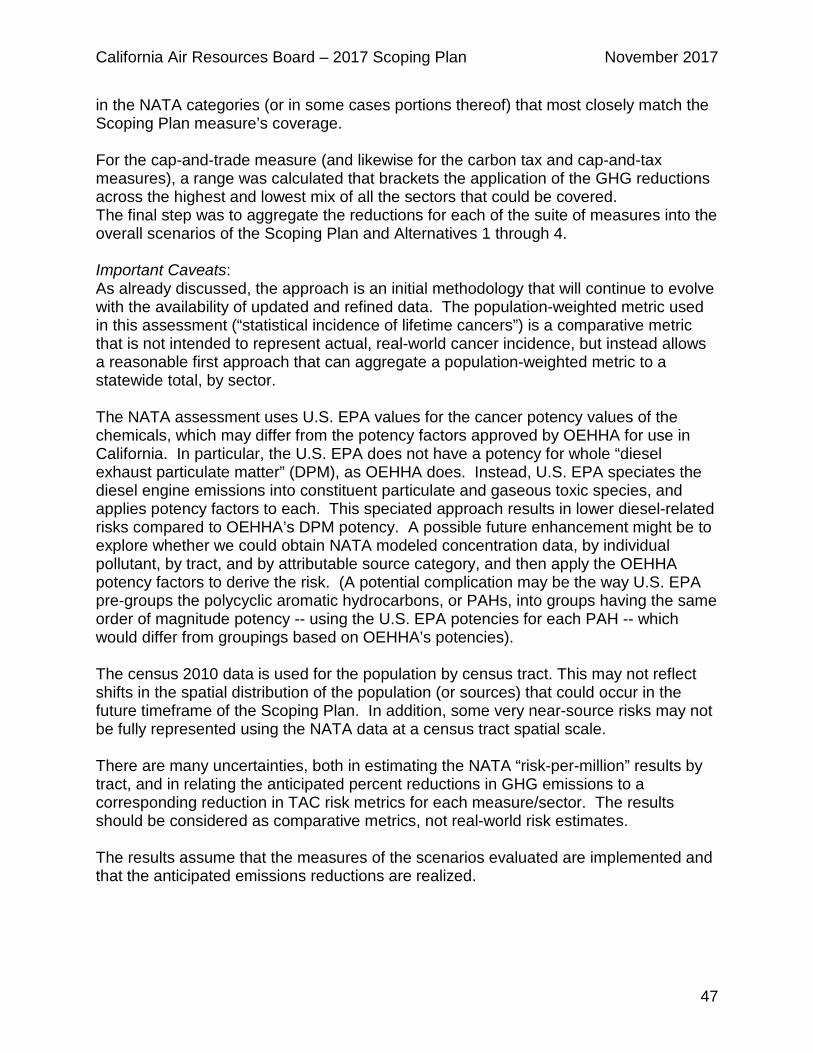
California Air Resources Board – 2017 Scoping Plan November 2017
47
in the NATA categories (or in some cases portions thereof) that most closely match the Scoping Plan measure’s coverage. For the cap-and-trade measure (and likewise for the carbon tax and cap-and-tax measures), a range was calculated that brackets the application of the GHG reductions across the highest and lowest mix of all the sectors that could be covered. The final step was to aggregate the reductions for each of the suite of measures into the overall scenarios of the Scoping Plan and Alternatives 1 through 4. Important Caveats: As already discussed, the approach is an initial methodology that will continue to evolve with the availability of updated and refined data. The population-weighted metric used in this assessment (“statistical incidence of lifetime cancers”) is a comparative metric that is not intended to represent actual, real-world cancer incidence, but instead allows a reasonable first approach that can aggregate a population-weighted metric to a statewide total, by sector. The NATA assessment uses U.S. EPA values for the cancer potency values of the chemicals, which may differ from the potency factors approved by OEHHA for use in California. In particular, the U.S. EPA does not have a potency for whole “diesel exhaust particulate matter” (DPM), as OEHHA does. Instead, U.S. EPA speciates the diesel engine emissions into constituent particulate and gaseous toxic species, and applies potency factors to each. This speciated approach results in lower diesel-related risks compared to OEHHA’s DPM potency. A possible future enhancement might be to explore whether we could obtain NATA modeled concentration data, by individual pollutant, by tract, and by attributable source category, and then apply the OEHHA potency factors to derive the risk. (A potential complication may be the way U.S. EPA pre-groups the polycyclic aromatic hydrocarbons, or PAHs, into groups having the same order of magnitude potency -- using the U.S. EPA potencies for each PAH -- which would differ from groupings based on OEHHA’s potencies). The census 2010 data is used for the population by census tract. This may not reflect shifts in the spatial distribution of the population (or sources) that could occur in the future timeframe of the Scoping Plan. In addition, some very near-source risks may not be fully represented using the NATA data at a census tract spatial scale. There are many uncertainties, both in estimating the NATA “risk-per-million” results by tract, and in relating the anticipated percent reductions in GHG emissions to a corresponding reduction in TAC risk metrics for each measure/sector. The results should be considered as comparative metrics, not real-world risk estimates. The results assume that the measures of the scenarios evaluated are implemented and that the anticipated emissions reductions are realized.
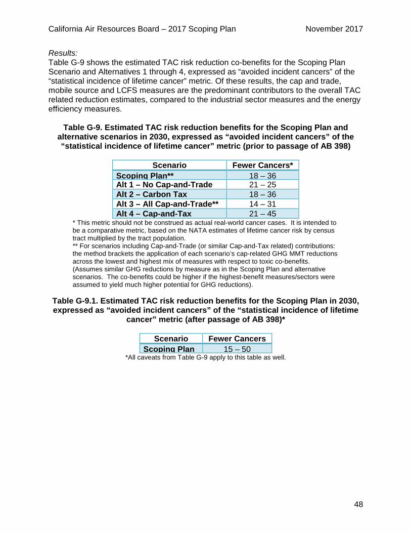
California Air Resources Board – 2017 Scoping Plan November 2017
48
Results: Table G-9 shows the estimated TAC risk reduction co-benefits for the Scoping Plan Scenario and Alternatives 1 through 4, expressed as “avoided incident cancers” of the “statistical incidence of lifetime cancer” metric. Of these results, the cap and trade, mobile source and LCFS measures are the predominant contributors to the overall TAC related reduction estimates, compared to the industrial sector measures and the energy efficiency measures.
Table G-9. Estimated TAC risk reduction benefits for the Scoping Plan and alternative scenarios in 2030, expressed as “avoided incident cancers” of the “statistical incidence of lifetime cancer” metric (prior to passage of AB 398)
Scenario Fewer Cancers*
Scoping Plan** 18 – 36 Alt 1 – No Cap-and-Trade 21 – 25 Alt 2 – Carbon Tax 18 – 36 Alt 3 – All Cap-and-Trade** 14 – 31 Alt 4 – Cap-and-Tax 21 – 45
* This metric should not be construed as actual real-world cancer cases. It is intended to be a comparative metric, based on the NATA estimates of lifetime cancer risk by census tract multiplied by the tract population. ** For scenarios including Cap-and-Trade (or similar Cap-and-Tax related) contributions: the method brackets the application of each scenario’s cap-related GHG MMT reductions across the lowest and highest mix of measures with respect to toxic co-benefits. (Assumes similar GHG reductions by measure as in the Scoping Plan and alternative scenarios. The co-benefits could be higher if the highest-benefit measures/sectors were assumed to yield much higher potential for GHG reductions).
Table G-9.1. Estimated TAC risk reduction benefits for the Scoping Plan in 2030, expressed as “avoided incident cancers” of the “statistical incidence of lifetime
cancer” metric (after passage of AB 398)*
Scenario Fewer Cancers Scoping Plan 15 – 50
*All caveats from Table G-9 apply to this table as well.
California Air Resources Board – 2017 Scoping Plan November 2017
49
References Air Resources Board (ARB) (2010) Estimate of Premature Deaths Associated with Fine Particle Pollution (PM2.5) in California Using a U.S. Environmental Protection Agency Methodology. https://www.arb.ca.gov/research/health/pm-mort/pm-report_2010.pdf Basu R, Wen-Ying F, Ostro B (2008) Characterizing temperature and mortality in nine California counties. Epidemiology. doi:10.1097/EDE.0b013e31815c1da7 Bell et al. (2008) Seasonal and Regional Short-term Effects of Fine Particles on Hospital Admissions in 202 US Counties, 1999–2005. Am J Epidemiol. 168(11): 1301–1310. https://www.ncbi.nlm.nih.gov/pmc/articles/PMC2732959/ Caltrans Strategic Management Plan 2015-2020 (CSMP) (2015). Cayan D., Tyree M., Dettinger M., Hidalgo M., Das T., Maurer E., Bromirski P., Graham N., Flick R. (2009) Climate change scenarios and sea level rise estimates for the California 2009 climate change scenarios Assessment. California Energy Commission, Sacramento, CEC-500-2009-014-F. Franco, G., D.R. Cayan, S. Moser, M. Hanemann, and M.-A. Jones (2011) Second California Assessment: Integrated climate change impacts assessment of natural and managed systems. Guest editorial. Climatic Change, 87 (Supplement 1): S7-S20. Green R., Basu R., Malig B., Broadwin R., Kim J., Ostro B. (2010) The effect of temperature on hospital admissions in nine California counties. Int J Public Health. doi:10.1007/s00038-009-0076-0. Krewski et al. (2009) Extended Follow-Up and Spatial Analysis of the American Cancer Society Study Linking Particulate Air Pollution and Mortality. Health Effects Institute Research Report 140. https://ephtracking.cdc.gov/docs/RR140-Krewski.pdf. Heath, G.A.; Granvold, P.W.; Hoats, A.S.; Nazaroff, W.W. (2006) Intake fraction assessment of the air pollutant exposure implications of a shift toward distributed electricity generation. Atmos. Environ. 40, 7164–7177. Ito et al. (2007) Characterization of PM2.5, gaseous pollutants, and meteorological interactions in the context of time-series health effects models. J Expo Sci Environ Epidemiol. Vol. 17 Suppl 2: S45-60. http://www.nature.com/jes/journal/v17/n2s/full/7500627a.html. Mahmud A, Tyree M, Cayan D, Motallebi N, Kleeman M (2008) Statistical downscaling of climate change impacts on ozone concentrations in California. J Geophys Res. doi:10.1029/2007JD009534.
California Air Resources Board – 2017 Scoping Plan November 2017
50
Maizlish, N. (2016a) Increasing Walking, Cycling, and Transit: Improving Californians’ Health, Saving costs, and Reducing Greenhouse Gases. Office of Health Equity, California Department of Public Health. http://www.cdph.ca.gov/programs/Documents/IncreasingWalkingCyclingTransitFinalReport2016rev2017-01-28.pdf Maizlish, N. (2016b) Integrated Transport and Health Impact Model (ITHIM): A Guide to Operation, Calibration and Integration with Travel Demand Models. California Spreadsheet Version December 12, 2016. Maizlish N, Linesch N, Woodcock J. Health and greenhouse gas mitigation benefits of ambitious expansion of cycling, walking, and transit in California. Journal of Transport and Health. 2017; doi: 10.1016/j.jth.2017.04.011 Marshall, J.D.; Nazaroff, W.W. (2004) Using Intake Fraction to Guide ARB Policy Choices: The Case of Particulate Matter, ARB Contract Number 04-312. http://depts.washington.edu/airqual/reports/MARSHALL%20and%20NAZAROFF%20-%20IF%20and%20PM.doc. Office of Environmental Health Hazard Assessment (2015) “Air Toxics Hot Spots Program Guidance Manual for Preparation of Health Risk Assessments”, March 2015. U.S. Environmental Protection Agency (2011) National Air Toxics Assessment 2011 (NATA) available at https://www.epa.gov/national-air-toxics-assessment/2011-national-air-toxics-assessment which is referenced from this U.S. EPA website: https://www.epa.gov/national-air-toxics-assessment.


