Appendix G Analytical Studies of Columns

G-1

G.1 Introduction

Analytical parametric studies were performed to evaluate a number of issues related to the use of ASTM A1035 steel as longitudinal and transverse reinforcement in structural concrete columns. The current AASHTO requirements for spacing of A1035 spirals were also examined and recommended revisions are made. The confined model proposed by Razvi and Saatcioglu (1999) was used in the reported analyses. Validation of this model is reported prior to presentation of the results from the analytical parametric studies. G.2 Verification of Confined Model

A concrete model by Razvi and Saatcioglu (1999) was implemented to define the stress-strain relationships for confined and unconfined concrete. This model is based on an experimental program involving 46 columns tested by its developers and test results from previous studies. In total, the model was calibrated against 92 test data points, which were from square (core dimensions ranging from approximately 7-13/16”×7-13/16” to 8-13/16” ”×8-13/16”) and circular columns (with core diameters ranging approximately from 8” to 8-13/16”) with concrete compressive strengths ranging from 7.4 ksi to 15.3 ksi. The model was further evaluated through the use of data from two other research programs involving columns that were larger than those used in the original model verifications. Pessiki and Graybeal (2000) performed concentric axial compression tests on eight large-scale columns. Four test specimens were of 24-inch diameters and were 96 inches long, and four were of 14-inch diameters and were 56 inches long. All the specimens had a 2-inch concrete cover. The nominal yield strength of the spiral reinforcement ranged from 78 ksi to 140 ksi. The diameter of the spiral was 0.35 inches in each specimen. The concrete compressive strength was designed to be 8 ksi. A study conducted by Richart and Brown (1934) at the University of Illinois was also used to provide additional data points. As part of this study, over 500 columns were tested. Considering that the concrete was quite weak by current standards (the compressive strengths were between 1540 psi and 3810 psi), only the results from the largest tested columns were included. The selected columns had outer diameters of 24 inches and 32 inches with 2 inches of cover. The diameters of the spirals were 5/16 in. and 3/8 in. at spacing of 1.1975 in. and 1.185 in., respectively. The yield strengths of the spirals were 44.5 ksi and 41.3 ksi, and the longitudinal bars had yield strengths of 50.4 ksi and 45.3 ksi. The yield strengths correspond to the stress at a strain of 0.005. G.2.1 Results and Observations

The computed and measured confined concrete strengths could be compared directly for the tests conducted and/or reported by Razvi and Saatcioglu (1999) and for the specimens tested by Pessiki and Graybeal (2000). However, the 1934 report by Richart and Brown did not provide enough information for calculating the confined concrete strengths. For these specimens, the axial load capacity was computed as the sum of the contribution of cover concrete, core concrete, and longitudinal bars by applying Eq. G-1.

P = f 'c Ag − Ac( ) + f 'cc Ac − As( ) + As f y (G-1)

G-2

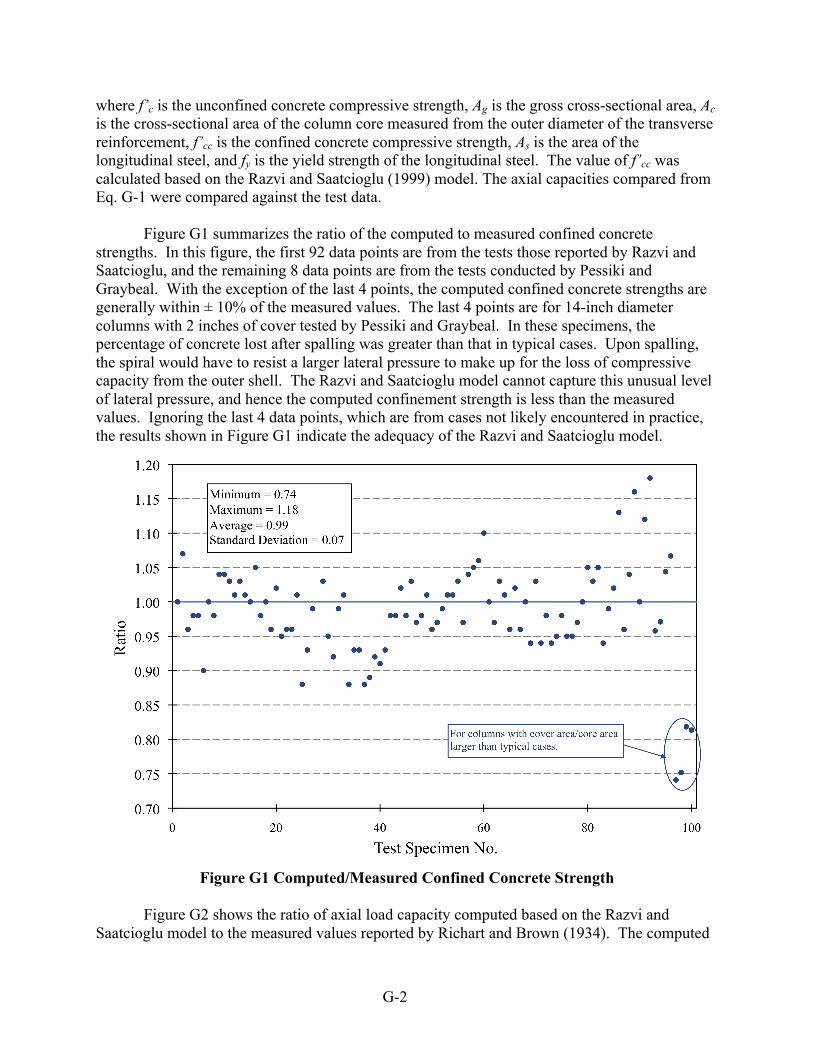
where f’c is the unconfined concrete compressive strength, Ag is the gross cross-sectional area, Ac is the cross-sectional area of the column core measured from the outer diameter of the transverse reinforcement, f’cc is the confined concrete compressive strength, As is the area of the longitudinal steel, and fy is the yield strength of the longitudinal steel. The value of f’cc was calculated based on the Razvi and Saatcioglu (1999) model. The axial capacities compared from Eq. G-1 were compared against the test data.

Figure G1 summarizes the ratio of the computed to measured confined concrete strengths. In this figure, the first 92 data points are from the tests those reported by Razvi and Saatcioglu, and the remaining 8 data points are from the tests conducted by Pessiki and Graybeal. With the exception of the last 4 points, the computed confined concrete strengths are generally within ± 10% of the measured values. The last 4 points are for 14-inch diameter columns with 2 inches of cover tested by Pessiki and Graybeal. In these specimens, the percentage of concrete lost after spalling was greater than that in typical cases. Upon spalling, the spiral would have to resist a larger lateral pressure to make up for the loss of compressive capacity from the outer shell. The Razvi and Saatcioglu model cannot capture this unusual level of lateral pressure, and hence the computed confinement strength is less than the measured values. Ignoring the last 4 data points, which are from cases not likely encountered in practice, the results shown in Figure G1 indicate the adequacy of the Razvi and Saatcioglu model.

Figure G1 Computed/Measured Confined Concrete Strength

Figure G2 shows the ratio of axial load capacity computed based on the Razvi and

Saatcioglu model to the measured values reported by Richart and Brown (1934). The computed

G-3

capacities are appreciably larger than the measured values. This difference may be attributed to several reasons, the most significant of which is contributed to lack of information about the level of stress in the longitudinal and transverse reinforcement at failure. The Razvi and Saatcioglu model is based on the premise that transverse steel yields. Additionally, the axial load was computed by using the yield strength of the longitudinal bars. If the reinforcing bars in the test specimens did not yield prior to failure, the calculated axial capacities would overestimate the reported failure loads. With the lack of adequate information about the level of stress in the specimens tested by Richart and Brown, the results shown in Figure G2 can neither prove nor disprove the adequacy of the Razvi and Saatcioglu model.

Figure G2 Computed/ Measured Axial Column Capacity

The comparisons made in Figure G1 demonstrate that the Razvi and Saatcioglu model can reasonably match the measured confined concrete strengths. This model is deemed sufficiently accurate for the parametric studies reported in this chapter. D.2.2 Epilogue

The influence of modeling of confined concrete is examined in this section. The axial load in most bridge columns is on the order of 0.05f’cAg (Mander, 1994) where f’c is the concrete compressive strength and Ag is the gross cross-sectional area of the column. Figure G3 illustrates the interaction diagrams for a typical column with various sizes and types of spirals. Up to the balance point, the interaction diagrams for cases in which the entire cross-section is

G-4

modeled as unconfined concrete are nearly identical to cases that account for confined concrete. Even for axial loads (0.1 or 0.2f’cAg) larger than what most bridge columns would experience, no discernable differences can be seen. Therefore, the flexural capacity of columns for a practical range of axial loads is not affected by how the confined concrete is modeled.

Figure G3 Interaction Diagram for a 24” diameter column with f’c = 10 ksi

The effects of confinement and post-peak behavior of confined concrete were also

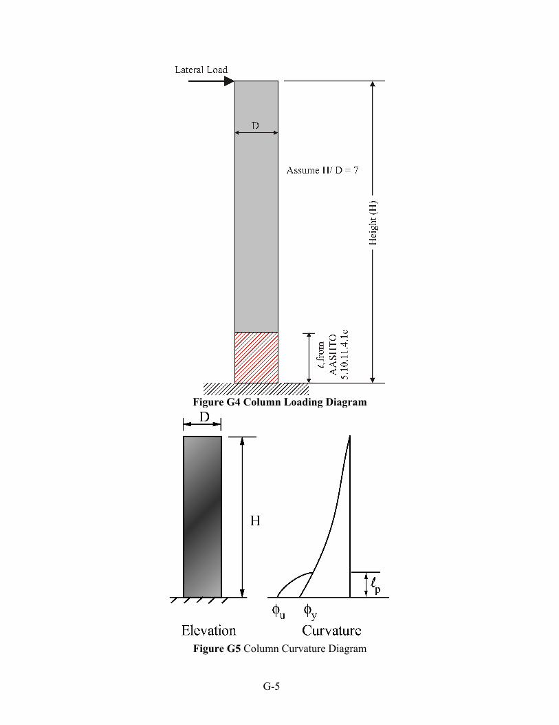
evaluated in terms of the moment-curvature responses and behavior under ultimate conditions, both of which are associated with lateral drift which is primarily a seismic consideration. The lateral load-deflection of a 14-ft cantilever shown in Figure G4 was used for this purpose.

The height to column depth was taken as 7 to ensure that the calculated deflections would be dominated by flexural deformations. The sum of elastic deformations (δy) and plastic deformations (δp) will be the lateral deflection. The elastic deformation is directly derived from

structural analysis, which is

φH 3

3 in which φ is the curvature at the base and H is the column

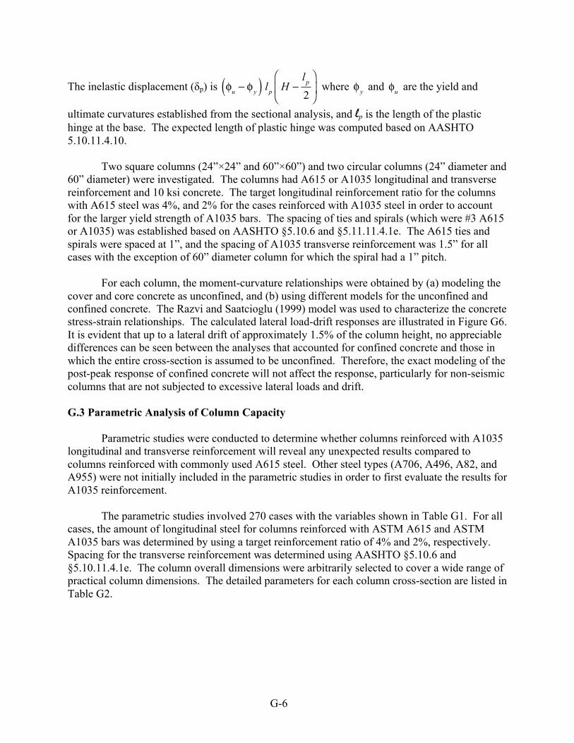
height. The curvature depends on the moment and elastic modulus. The curvatures were obtained from the sectional analysis of the column conducted by XTRACT (Imbsen, 2007). The second component of the displacement (δp, i.e., the plastic deformation) was computed based on the curvature distribution shown in Figure G5.

G-5

Figure G4 Column Loading Diagram

Figure G5 Column Curvature Diagram

G-6

The inelastic displacement (δp) is φu − φ y( ) lp H −

lp

2

⎛

⎝⎜

⎞

⎠⎟ where

φ y and φu are the yield and

ultimate curvatures established from the sectional analysis, and lp is the length of the plastic hinge at the base. The expected length of plastic hinge was computed based on AASHTO 5.10.11.4.10.

Two square columns (24”×24” and 60”×60”) and two circular columns (24” diameter and 60” diameter) were investigated. The columns had A615 or A1035 longitudinal and transverse reinforcement and 10 ksi concrete. The target longitudinal reinforcement ratio for the columns with A615 steel was 4%, and 2% for the cases reinforced with A1035 steel in order to account for the larger yield strength of A1035 bars. The spacing of ties and spirals (which were #3 A615 or A1035) was established based on AASHTO §5.10.6 and §5.11.11.4.1e. The A615 ties and spirals were spaced at 1”, and the spacing of A1035 transverse reinforcement was 1.5” for all cases with the exception of 60” diameter column for which the spiral had a 1” pitch.

For each column, the moment-curvature relationships were obtained by (a) modeling the cover and core concrete as unconfined, and (b) using different models for the unconfined and confined concrete. The Razvi and Saatcioglu (1999) model was used to characterize the concrete stress-strain relationships. The calculated lateral load-drift responses are illustrated in Figure G6. It is evident that up to a lateral drift of approximately 1.5% of the column height, no appreciable differences can be seen between the analyses that accounted for confined concrete and those in which the entire cross-section is assumed to be unconfined. Therefore, the exact modeling of the post-peak response of confined concrete will not affect the response, particularly for non-seismic columns that are not subjected to excessive lateral loads and drift. G.3 Parametric Analysis of Column Capacity

Parametric studies were conducted to determine whether columns reinforced with A1035 longitudinal and transverse reinforcement will reveal any unexpected results compared to columns reinforced with commonly used A615 steel. Other steel types (A706, A496, A82, and A955) were not initially included in the parametric studies in order to first evaluate the results for A1035 reinforcement.

The parametric studies involved 270 cases with the variables shown in Table G1. For all cases, the amount of longitudinal steel for columns reinforced with ASTM A615 and ASTM A1035 bars was determined by using a target reinforcement ratio of 4% and 2%, respectively. Spacing for the transverse reinforcement was determined using AASHTO §5.10.6 and §5.10.11.4.1e. The column overall dimensions were arbitrarily selected to cover a wide range of practical column dimensions. The detailed parameters for each column cross-section are listed in Table G2.

G-7

(a) 24-inch diameter “seismic column”

(b) 60-inch diameter “seismic column”

(c) 24-inch square “seismic” column

(d) 60-inch square “seismic column”

Figure G6 Lateral Load – Drift Response

Table G1 Variables for Column Parametric Studies Variable Value/Description

Column Type Square tied columns designed and detailed for seismic loads Circular spirally reinforced columns used in non-seismic regions Circular spirally reinforced columns for bridges subjected to seismic loads

Type of Reinforcement

ASTM A615 with fy = 60 ksi and ASTM A1035 with fy = 120 ksi (for longitudinal and transverse bars)

Column Size Square column dimension or diameter =18, 24, 36, 48, 60 in.

Transverse Reinforcement #3, #4, and #5

Concrete Strength f’c = 5, 10, 15 ksi

G-8

Table G2 Column Details (Square Seismic Columns) Transverse Steel Longitudinal Steel A615 A1035 Case f'c (ksi)

A615 A1035 Size & Spacing

No. of Crossties

Size & Spacing

No. of Crossties

12#10 8#10 #3 @ 1.0" 0 #3 @ 2.5" 0 12#10 8#10 #4 @ 2.0" 0 #4 @ 4.0" 0 5 12#10 8#10 #5 @ 3.5" 0 #5 @ 4.0" 0 12#10 8#10 #3 @ 1.0" 0 #3 @ 1.0" 0 12#10 8#10 #4 @ 1.0" 0 #4 @ 2.0" 0 10 12#10 8#10 #5 @ 1.5" 0 #5 @ 3.5" 0 12#10 8#10 #3 @ 1.0" 0 #3 @ 1.0" 0 12#10 8#10 #4 @ 1.0" 0 #4 @ 1.5" 0

18”

15 12#10 8#10 #5 @ 1.0" 0 #5 @ 2.5" 0 20#10 12#10 #3 @ 1.5" 1 #3 @ 3.0" 1 20#10 12#10 #4 @ 2.5" 1 #4 @ 4.0" 1 5 20#10 12#10 #5 @ 4.0" 1 #5 @ 4.0" 1 20#10 12#10 #3 @ 1.0" 1 #3 @ 1.5" 1 20#10 12#10 #4 @ 1.0" 1 #4 @ 2.5" 1 10 20#10 12#10 #5 @ 2.0" 1 #5 @ 4.0" 1 20#10 12#10 #3 @ 1.0" 1 #3 @ 1.0" 1 20#10 12#10 #4 @ 1.0" 1 #4 @ 1.5" 1

24”

15 20#10 12#10 #5 @ 1.0" 1 #5 @ 2.5" 1 44#10 20#10 #3 @ 1.0" 2 #3 @ 2.5" 2 44#10 20#10 #4 @ 2.0" 2 #4 @ 4.0" 2 5 44#10 20#10 #4 @ 3.5" 2 #5 @ 4.0" 2 44#10 20#10 #3 @ 1.0" 2 #3 @ 1.0" 2 44#10 20#10 #4 @ 1.0" 2 #4 @ 2.0" 2 10 44#10 20#10 #5 @ 1.5" 2 #5 @ 3.5" 2 44#10 20#10 #3 @ 1.0" 2 #3 @ 1.0" 2 44#10 20#10 #4 @ 1.0" 2 #4 @ 1.5" 2

36”

15 44#10 20#10 #5 @ 1.0" 2 #5 @ 2.5" 2 76#10 36#10 #3 @ 1.0" 4 #3 @ 2.5" 4 76#10 36#10 #4 @ 2.5" 4 #4 @ 4.0" 4 5 76#10 36#10 #5 @ 4.0" 4 #5 @ 4.0" 4 76#10 36#10 #3 @ 1.0" 4 #3 @ 1.0" 4 76#10 36#10 #4 @ 1.0" 4 #4 @ 2.5" 4 10 76#10 36#10 #5 @ 2.0" 4 #5 @ 4.0" 4 76#10 36#10 #3 @ 1.0" 4 #3 @ 1.0" 4 76#10 36#10 #4 @ 1.0" 4 #4 @ 1.5" 4

48”

15 76#10 36#10 #5 @ 1.0" 4 #5 @ 2.5" 4

112#10 60#10 #3 @ 1.5" 6 #3 @ 3.0" 6 112#10 60#10 #4 @ 2.5" 6 #4 @ 4.0" 6 5 112#10 60#10 #4 @ 3.5" 6 #5 @ 4.0" 6 112#10 60#10 #3 @ 1.0" 6 #3 @ 1.5" 6 112#10 60#10 #4 @ 1.0" 6 #4 @ 2.5" 6 10 112#10 60#10 #5 @ 1.5" 6 #5 @ 3.5" 6 112#10 60#10 #3 @ 1.0" 6 #3 @ 1.0" 6 112#10 60#10 #4 @ 1.0" 6 #4 @ 1.5" 6

60”

15 112#10 60#10 #5 @ 1.0" 6 #5 @ 2.5" 6

G-9

Table G2 (Cont.) Column Details (Spiral Seismic Columns) Transverse Steel Longitudinal Steel

A615 A1035 Case f'c (ksi) A615 A1035 Size & Spacing Size & Spacing 7#11 6#11 #3 @ 1.5" #3 @ 3.0" 7#11 6#11 #4 @ 3.0" #4 @ 4.0" 5 7#11 6#11 #5 @ 4.0" #5 @ 4.0" 7#11 6#11 #3 @ 1.0" #3 @ 1.5" 7#11 6#11 #4 @ 1.5" #4 @ 3.0" 10 7#11 6#11 #5 @ 2.0" #5 @ 4.0" 7#11 6#11 #3 @ 1.0" #3 @ 1.0" 7#11 6#11 #4 @ 1.0" #4 @ 2.0"

18”

15 7#11 6#11 #5 @ 1.5" #5 @ 3.0"

12#11 8#11 #3 @ 1.5" #3 @ 3.5" 12#11 8#11 #4 @ 3.0" #4 @ 4.0" 5 12#11 8#11 #5 @ 4.0" #5 @ 4.0" 12#11 8#11 #3 @ 1.0" #3 @ 1.5" 12#11 8#11 #4 @ 1.5" #4 @ 3.0" 10 12#11 8#11 #5 @ 2.0" #5 @ 4.0" 12#11 8#11 #3 @ 1.0" #3 @ 1.0" 12#11 8#11 #4 @ 1.0" #4 @ 2.0"

24”

15 12#11 8#11 #5 @ 1.5" #5 @ 3.0" 26#11 13#11 #3 @ 1.0" #3 @ 2.5" 26#11 13#11 #4 @ 2.0" #4 @ 4.0" 5 26#11 13#11 #5 @ 3.5" #5 @ 4.0" 26#11 13#11 #3 @ 1.0" #3 @ 1.0" 26#11 13#11 #4 @ 1.0" #4 @ 2.0" 10 26#11 13#11 #5 @ 1.5" #5 @ 3.5" 26#11 13#11 #3 @ 1.0" #3 @ 1.0" 26#11 13#11 #4 @1.0" #4 @ 1.5"

36”

15 26#11 13#11 #5 @1.0" #5 @ 2.0" 46#11 23#11 #3 @ 1.0" #3 @ 1.5" 46#11 23#11 #4 @ 1.5" #4 @ 3.0" 5 46#11 23#11 #5 @ 2.5" #5 @ 4.0" 46#11 23#11 #3 @ 1.0" #3 @ 1.0" 46#11 23#11 #4 @ 1.0" #4 @ 1.5" 10 46#11 23#11 #5 @ 1.0" #5 @ 2.5" 46#11 23#11 #3 @ 1.0" #3 @ 1.0" 46#11 23#11 #4 @1.0" #4 @ 1.0"

48”

15 46#11 23#11 #5 @1.0" #5 @ 1.5" 72#11 36#11 #3 @ 1.0" #3 @ 1.5" 72#11 36#11 #4 @ 1.0" #4 @ 2.5" 5 72#11 36#11 #5 @ 2.0" #5 @ 4.0" 72#11 36#11 #3 @ 1.0" #3 @ 1.0" 72#11 36#11 #4 @ 1.0" #4 @ 1.0" 10 72#11 36#11 #5 @ 1.0" #5 @ 2.0" 72#11 36#11 #3 @ 1.0" #3 @ 1.0" 72#11 36#11 #4 @1.0" #4 @ 1.0"

60”

15 72#11 36#11 #5 @1.0" #5 @ 1.0"

G-10

Table G2 (Cont.) Column Details (Spiral Non-seismic Columns) Transverse Steel Longitudinal Steel

A615 A1035 Case f'c (ksi) A615 A1035 Size & Spacing Size & Spacing 7#11 6#11 #3 @ 1.5" #3 @ 3.0" 7#11 6#11 #4 @ 3.0" #4 @ 6.0" 5 7#11 6#11 #5 @ 4.5" #5 @ 6.0" 7#11 6#11 #3 @ 1.0" #3 @ 1.5" 7#11 6#11 #4 @ 1.5" #4 @ 3.0" 10 7#11 6#11 #5 @ 2.0" #5 @ 4.5" 7#11 6#11 #3 @ 1.0" #3 @ 1.0" 7#11 6#11 #4 @ 1.0" #4 @ 2.0"

18”

15 7#11 6#11 #5 @ 1.5" #5 @ 3.0"

12#11 8#11 #3 @ 1.5" #3 @ 3.5" 12#11 8#11 #4 @ 3.0" #4 @ 6.0" 5 12#11 8#11 #5 @ 4.5" #5 @ 6.0" 12#11 8#11 #3 @ 1.0" #3 @ 1.5" 12#11 8#11 #4 @ 1.5" #4 @ 3.0" 10 12#11 8#11 #5 @ 2.0" #5 @ 5.0" 12#11 8#11 #3 @ 1.0" #3 @ 1.0" 12#11 8#11 #4 @ 1.0" #4 @ 2.0"

24”

15 12#11 8#11 #5 @ 1.5" #5 @ 3.0" 26#11 13#11 #3 @ 1.5" #3 @ 3.5" 26#11 13#11 #4 @ 3.0" #4 @ 6.0" 5 26#11 13#11 #5 @ 4.5" #5 @ 6.0" 26#11 13#11 #3 @ 1.0" #3 @ 1.5" 26#11 13#11 #4 @ 1.5" #4 @ 3.0" 10 26#11 13#11 #5 @ 2.5" #5 @ 5.0" 26#11 13#11 #3 @ 1.0" #3 @ 1.0" 26#11 13#11 #4 @ 1.0" #4 @ 2.0"

36”

15 26#11 13#11 #5 @ 1.5" #5 @ 3.0" 46#11 23#11 #3 @ 1.5" #3 @ 3.5" 46#11 23#11 #4 @ 3.0" #4 @ 6.0" 5 46#11 23#11 #5 @ 5.0" #5 @ 6.0" 46#11 23#11 #3 @ 1.0" #3 @ 1.5" 46#11 23#11 #4 @ 1.5" #4 @ 3.0" 10 46#11 23#11 #5 @ 2.5" #5 @ 5.0" 46#11 23#11 #3 @ 1.0" #3 @ 1.0" 46#11 23#11 #4 @ 1.0" #4 @ 2.0"

48”

15 46#11 23#11 #5 @ 1.5" #5 @ 3.0" 72#11 36#11 #3 @ 1.5" #3 @ 3.5" 72#11 36#11 #4 @ 3.0" #4 @ 6.0" 5 72#11 36#11 #5 @ 5.0" #5 @ 6.0" 72#11 36#11 #3 @ 1.0" #3 @ 1.5" 72#11 36#11 #4 @ 1.5" #4 @ 3.0" 10 72#11 36#11 #5 @ 2.5" #5 @ 5.0" 72#11 36#11 #3 @ 1.0" #3 @ 1.0" 72#11 36#11 #4 @ 1.0" #4 @ 2.0"

60”

15 72#11 36#11 #5 @ 1.5" #5 @ 3.5"

G-11

A fiber analysis program called XTRACT (Imbsen, 2007) was used to perform detailed cross-sectional fiber analyses. The stress-strain relationship for ASTM A615 reinforcement was based on an available model that replicates the behavior of such bars with the following values: yield strength = 60 ksi, ultimate strength = 90 ksi, strain at the onset of strain hardening = 0.008, and fracture strain = 0.09. A user-defined material model, in which discrete strain and stress data points were input, was used to represent the stress-strain relationship of ASTM A1035. The strain and stress values for each data point were established from the Ramberg-Osgood function shown in Eq. G-2.

fs = Esεs A+1− A

1+ Bεs( )C⎡⎣⎢

⎤⎦⎥

1/C

⎧

⎨⎪⎪

⎩⎪⎪

⎫

⎬⎪⎪

⎭⎪⎪

≤ fu (G-2)

in which A = 0.0100, B = 166, C = 1.8000, fu = 182 ksi, and Es = 29000 ksi.

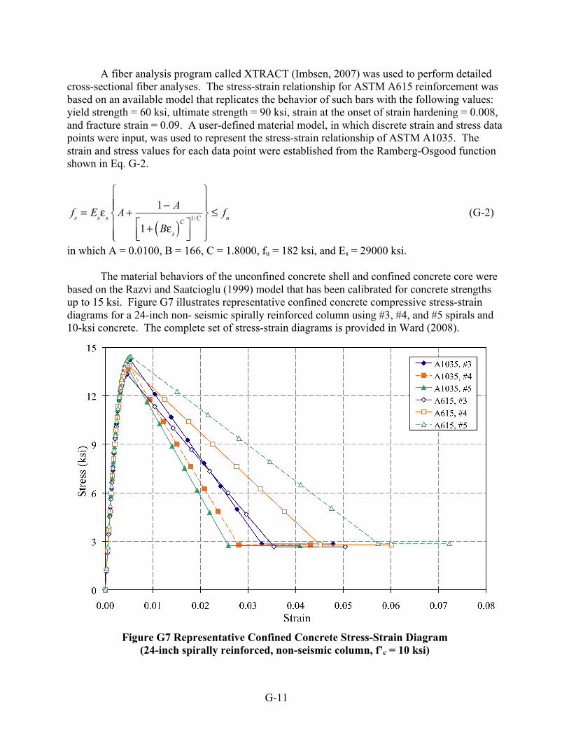
The material behaviors of the unconfined concrete shell and confined concrete core were based on the Razvi and Saatcioglu (1999) model that has been calibrated for concrete strengths up to 15 ksi. Figure G7 illustrates representative confined concrete compressive stress-strain diagrams for a 24-inch non- seismic spirally reinforced column using #3, #4, and #5 spirals and 10-ksi concrete. The complete set of stress-strain diagrams is provided in Ward (2008).

Figure G7 Representative Confined Concrete Stress-Strain Diagram

(24-inch spirally reinforced, non-seismic column, f’c = 10 ksi)

G-12

The confined stress-strain diagrams vary depending on the spacing of transverse steel. Considering that the spacing of A615 transverse reinforcement is smaller than that for A1035 steel, confined stresses for cases with A615 transverse reinforcement may be higher than those for cases with A1035 ties or spirals. For example, Figure G7 shows that the column with #5 A615 ties has a larger confined stress than the case with #5 A1035 because the spacing of A615 transverse reinforcement is 60% less than the spacing of A1035 ties (2” vs. 5”). The complete set of stress-strain diagrams reported elsewhere (Ward (2008)) suggest that the larger transverse reinforcing bars (#5 vs. #3) do not necessarily result in higher confinement stresses.

Representative moment-curvature relationships and axial load-moment (P-M) interaction diagrams are shown in Figures G8a and G8b, respectively, for a 24-inch diameter non-seismic spirally reinforced column using #3, #4, and #5 spirals and 10-ksi concrete. The moment-curvature responses were generated for an axial load corresponding to 0.1f’cAg where Ag is the column gross section area. The complete set of results is provided in Ward (2008). The variation in the moment-curvature diagrams is due to the differences in reinforcement ratios. The columns reinforced with A615 have more longitudinal bars and hence a greater stiffness. The reduced stiffness of columns with A1035 bars needs to be taken into account for design of bridges subjected to seismic loads. The different sizes of transverse steel do not significantly influence the moment-curvature relationships. This trend should be expected because the properties of concrete do not appreciably influence the response of members with small axial loads. Moreover, as discussed previously, the confined concrete properties are not affected by the size of transverse bars. The axial load-moment interaction diagrams (see Figure G8b) for columns with A615 and A1035 reinforcement vary primarily because of the larger amount of A615 longitudinal reinforcement. For a given type of steel (A615 or A1035), the size of transverse reinforcement does not affect the interaction diagrams.

The aforementioned results and discussions do not suggest any unexpected responses when A1035 steel is used. In comparison to A1035, the strengths and properties of other steel types (A706, A496, A82, and A955) are closer to the characteristics of A615. Since the responses of columns with A1035 steel do not suggest any unusual or unexpected trends, it was deemed unnecessary to perform similar parametric studies for A706, A496, A82, and A955.

G-13

(a) Representative Moment-Curvature Response

(b) Axial Load-Moment Interaction Diagram

Figure G8 – Representative Responses (24-inch spirally reinforced, non-seismic column, f’c = 10 ksi)

G-14

G.4 Spacing of Spiral Reinforcement

For cases that are not controlled by seismic requirements, the volumetric ratio of spiral

reinforcement must satisfy AASHTO §5.7.4.6 Eq. 5.7.4.6-1, i.e., .

Additionally, according to §5.10.6.2, the center-to-center spacing shall not exceed 6 times the diameter of the longitudinal bar or 6 inches. From a practical point of view, the spacing of spirals cannot be less than 1 inch or 1.33 times the maximum size of the aggregate (AASHTO

§5.10.6.2). This provision was reviewed to determine whether

accurately describes the confining ability of high-strength transverse steel.

The basis of AASHTO §5.7.4.6 Eq. 5.7.4.6-1 is to ensure that the axial load capacity of columns after spalling of the concrete cover is at least equal to the capacity before spalling. The axial load capacity before spalling is

Po = 0.85 f 'c ( Ag - As ) + As f y where Ag = the gross area of the column, As = the area of longitudinal steel, f’c = the compressive strength of the concrete, and fy = the yield strength of the longitudinal reinforcing bars. The use of fy for steel stress is valid as long as εs ≤εsh where εs = steel strain and εsh = strain at the onset of strain hardening. The corresponding capacity after spalling is

P ' = 0.85 f 'c+ 4.1 f2( )( Ac - As ) + As f y = 0.85 f 'c+ 4.1×2Asp f yh

bcs

⎛

⎝⎜

⎞

⎠⎟ ( Ac - As ) + As f y

P ' = 0.85 f 'c+ 2.05ρs f yh( )( Ac - As ) + As f y

where Ac = the area of confined core measured to the outer diameter of the spiral, fyh = the yield strength of the transverse reinforcing bars, and ρs = the volumetric ratio of the transverse steel. After spalling, confinement becomes effective; hence, the concrete strength has been increased due to confinement.

Set Po = P’ to calculate the minimum amount of spiral to ensure that the capacity after spalling is equal to that before spalling.

0.85 f 'c ( Ag - As ) + As f y = 0.85 f 'c+ 2.05ρs f yh( )( Ac - As ) + As f y from which

ρs =0.85 f 'c Ag − Ac( )2.05 f yh( Ac − As )

= 0.415

Ag

Ac

−1⎛

⎝⎜

⎞

⎠⎟

1−As

Ac

⎛

⎝⎜⎞

⎠⎟

f 'cf yh

. The value of

As

Ac

is small, e.g., per AASHTO

Spirals are assumed to yield

G-15

5.7.4.2 0.01≤

As

Ag

≤ 0.08 ; therefore,

As

Ac

will be between about 0.01 and 0.1 and may be ignored.

Hence, ρs = 0.415

Ag

Ac

−1⎛

⎝⎜

⎞

⎠⎟

f 'cf yh

. The value of 0.415 is arbitrarily increased to 0.45; therefore,

ρ s,min= 0.45

Ag

Ac

−1⎛

⎝⎜

⎞

⎠⎟

f 'cf yh

or ρs ≥ 0.45

Ag

Ac

−1⎛

⎝⎜

⎞

⎠⎟

f 'cf yh

as stated in AASHTO Eq. 5.7.4.6-1.

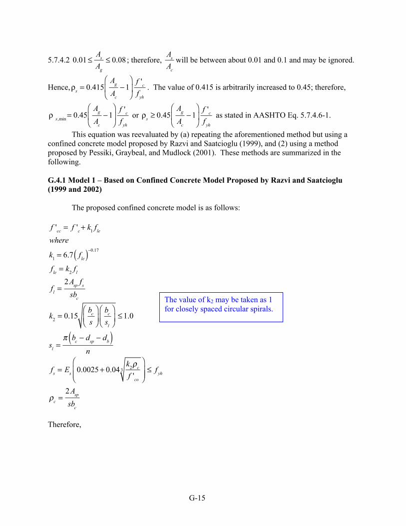
This equation was reevaluated by (a) repeating the aforementioned method but using a confined concrete model proposed by Razvi and Saatcioglu (1999), and (2) using a method proposed by Pessiki, Graybeal, and Mudlock (2001). These methods are summarized in the following. G.4.1 Model 1 – Based on Confined Concrete Model Proposed by Razvi and Saatcioglu (1999 and 2002)

The proposed confined concrete model is as follows:

f 'cc = f 'c+ k1 fle

where

k1 = 6.7 fle( )−0.17

fle = k2 fl

fl =2Asp fs

sbc

k2 = 0.15bc

s⎛

⎝⎜⎞

⎠⎟bc

sl

⎛

⎝⎜⎞

⎠⎟≤ 1.0

sl =π bc − dsp − db( )

n

fs = Es 0.0025+ 0.04k2ρc

f 'co

3⎛

⎝⎜⎜

⎞

⎠⎟⎟≤ f yh

ρc =2Asp

sbc

Therefore,

The value of k2 may be taken as 1 for closely spaced circular spirals.

G-16

f 'cc = f 'c+ 6.7 k2 fl( )0.83

where

fl =2Asp fs

sbc

k2 = 0.15bc

s⎛

⎝⎜⎞

⎠⎟bc

π bc − dsp − db( )n

⎡

⎣

⎢⎢⎢⎢⎢

⎤

⎦

⎥⎥⎥⎥⎥

≤ 1.0 & fs = Es 0.0025+ 0.04k2

2Asp

sbc

f 'co

3

⎛

⎝

⎜⎜⎜⎜⎜

⎞

⎠

⎟⎟⎟⎟⎟

≤ f yh

(G-3)

where f’cc = Confined concrete strength (MPa) f’c = Unconfined concrete strength (MPa) db = diameter of longitudinal bars (mm) bc = Core diameter (mm) Asp = Area of spirals (mm2) dsp = Diameter of spirals (mm) n = No. of longitudinal bars Es = Modulus of elasticity of spirals (MPa) fyh = Yield strength of spirals (MPa)

Calculate Po (Axial load capacity before spalling of cover) and P’ (Axial load capacity after spalling of cover) from the following equations.

Po = f 'c ( Ag − As ) + As f y

P ' = f 'cc ( Ac − As ) + As f y

Ag = Gross column area (mm2) As = Area of longitudinal bars (mm2) fy = yield strength of longitudinal bars (MPa) f’c = Unconfined concrete strength (MPa) f’cc = Confined concrete strength (MPa) computed from Eq. (G-3)

Set Po and P’ equal to each other.

f 'c ( Ag − As ) = f 'cc ( Ac − As ) (G-4)

For a given concrete compressive strength, column size, cover, longitudinal

reinforcement ratio, longitudinal bar size, spiral size, yield strength of spiral, and modulus of elasticity, iterate the value of “s” such that Eq. (G-4) is satisfied. Eq. (G-1) is used to compute f’cc.

Note: f’c and not 0.85f’c is used.

G-17

G.4.2 Model 2 – Based on Methodology Proposed by Pessiki, Graybeal, and Mudlock (2001)

The basis of this method is similar to that used for Method 1 with the exception of the confined concrete model.

Po = f 'c ( Ag − As ) + As f y

P ' = f 'cc ( Ac − As ) + As f y

Set Po and P’ equal to each other.

f 'c Ag − As( ) = f 'cc Ac − As( ) from which

f 'cc =

f 'c Ag − As( )Ac − As( )

f 'cc = f 'c+ 4.1 f2 from which f2 =

f 'cc− f 'c4.1

=f 'c Ag − Ac( )4.1 Ac − As( ) (G-5)

Use the following relationship to relate strain at confined concrete strength (εcc) to the

confined strength (f’cc) and unconfined strength (f’c).

εcc = εco 5f 'cc

f 'c− 4

⎛

⎝⎜⎞

⎠⎟= εco 5

f 'c Ag − As( )Ac − As( )

⎡

⎣⎢⎢

⎤

⎦⎥⎥

f 'c− 4

⎧

⎨

⎪⎪⎪

⎩

⎪⎪⎪

⎫

⎬

⎪⎪⎪

⎭

⎪⎪⎪

= εco 5Ag − As( )Ac − As( ) − 4

⎡

⎣

⎢⎢

⎤

⎦

⎥⎥

Use the dilation relationship εsp = 0.41εcc − 0.105εco to relate the lateral strain, which is

taken as the spiral strain (εsp) to axial strains.

Using an appropriate model, calculate fsp based on εsp. In this study, an elasto-plastic model was assumed for Gr. 60 A615 spirals, and Mast1 equation (2006) was used for A1035 spirals. The original paper did not provide a specific guideline for computing fsp.

Lateral confining pressure is f2 =

2Asp fsp

bcs in which f2 is computed from Eq. (G-5).

Therefore,

1

if εs ≤ 0.00241 fs = Esεs

if εs > 0.00241 fs = 170 −0.43

εs + 0.00188

Note: In the original paper, the dominator was taken as Ac.

G-18

f 'c Ag − Ac( )4.1 Ac − As( ) =

2Asp fsp

bcsfrom which s =

8.2Asp fsp Ac − As( )bc f 'c Ag − Ac( )

G.4.3 Parametric Study These two methods were used in a study aimed at evaluating the spacing of high-strength spiral reinforcement. Using the ASSHTO provision and the revised approach, the required spacings were computed for a number of columns with the parameters listed in Table G3. All the columns were reinforced with #9 longitudinal; the longitudinal reinforcement ratio was set equal to 1.5%. The cover to the spiral was taken as 1.5 in. The aim of this study was to evaluate the spacing of high-strength spiral reinforcement.

Table G3 Parameters for Transverse Spacing Study Variable Value/Description Concrete Compressive Strength* 5, 10, 15 ksi Spiral Yield Strength 60 ksi, 100 ksi, 120 ksi Column Diameter 18-80 in. (2 in. increments) Spiral Bar Size #3, #4, #5

* The strain at peak stress (εco) was taken as 0.0025. G.4.4 Results and Discussions

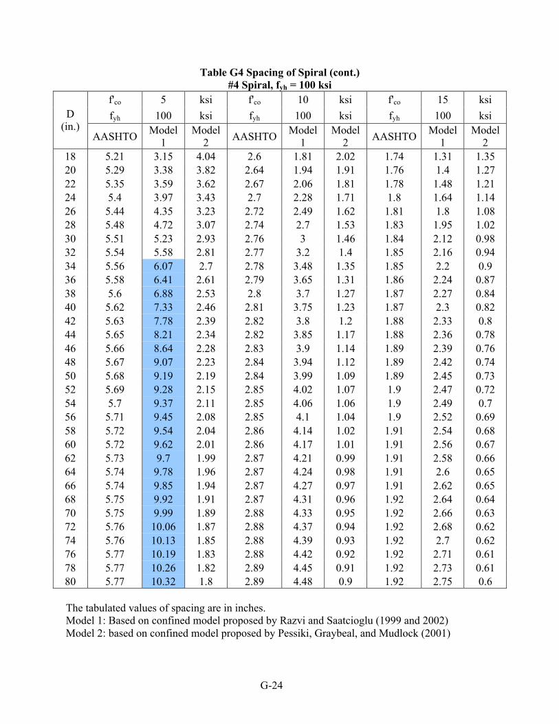
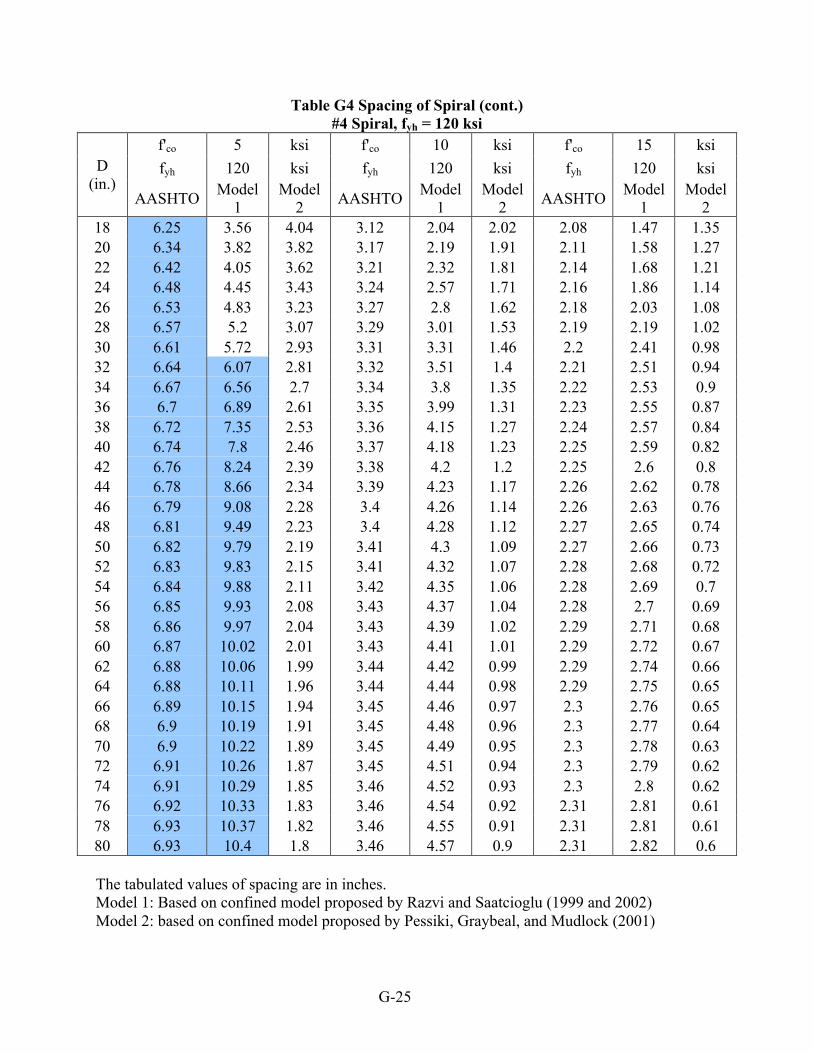
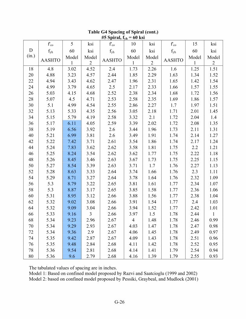
The calculated required spacings are summarized in Table G4. For a given concrete strength, the calculated spacing using any of the methods increases as the yield strength of the spiral increases. Additionally, as the size of the spiral increases, the calculated spacing increases. These trends are expected. For a number of cases (shaded in Table G4), the calculated spacings exceed the maximum limit of 6 inches. These cases involve columns with #4 spirals and 5-ksi concrete, and columns using #5 spirals and 5 and 10-ksi concrete. Most of these cases are for spirals with a yield strength of 100 ksi or 125 ksi. The calculated spacings in columns with a concrete strength of 15 ksi are below the maximum limit for all steel strengths and all spiral sizes. In terms of reducing the spiral spacing in columns cast with high-strength concrete, the use of larger, high-strength spirals is more efficient.

The three methods result in appreciably different spacing of spirals. As the column diameter is increased, the difference between the spacing from the different methods becomes more significant. The difference is most appreciable for columns with a concrete compressive strength of 5 ksi. Model 2 (based on Pessiki, Graybeal, and Mudlock’s confined concrete model) requires the smallest spacings, whereas Model 1 (based on Razvi-Saatcioglu’s confined concrete model) produces the largest spacings. This trend is exemplified in Figure G9, which illustrates the required spacing for a representative case involving 10-ksi concrete and 100-ksi #4 spiral. (The current AASHTO limits on minimum and maximum spacing (6” and 1”) are also shown in this figure.)

G-19

Figure G9 Required Spacing of Spiral from Different Models for a Representative Case

The trend of the spacings computed by Model 1 is expected. That is, as the column

diameter becomes larger, the difference between the core and gross areas diminishes; hence, the ratio of axial load capacity before and after spalling of cover approaches unity and spirals can be placed at larger spacings. From a confinement point of view, for an “infinitely” large column the spiral spacing is expected to become “infinitely large”. Model 1 accurately replicates this trend. For Model 2, spiral stress is reduced as the column becomes larger. Therefore, the spirals have to be placed at a smaller spacing to compensate for reduced lateral confining stress (f2 in Eq. (G-5)). The spacings computed by AASHTO Eq. 5.7.4.6-1 are not appreciably affected by the column size because the confined concrete core strength is a function of f’c (unconfined concrete strength) and Ag/Ac, neither of which is changed as appreciably as the other parameters in Models 1 and 2.

The difference between the spacings from different methods becomes more pronounced as the column diameter increases. Unfortunately, the available test data do not include test results for columns larger than 24 inches because of the large amount of axial force required to test large columns. For instance, approximately a 5-million pound universal machine will be required to test a 30-inch diameter column reinforced with 1.5% A615 longitudinal steel.

G-20

Table G4 Spacing of Spiral #3 Spiral, fyh = 60 ksi

f'co 5 ksi f'co 10 ksi f'co 15 ksi fyh 60 ksi fyh 60 ksi fyh 60 ksi D

(in.) AASHTO Model

1 Model

2 AASHTO Model 1

Model 2 AASHTO Model

1 Model

2 18 1.73 1.5 1.6 0.87 0.86 0.8 0.58 0.58 0.53 20 1.76 1.61 1.62 0.88 0.92 0.81 0.59 0.61 0.54 22 1.78 1.71 1.64 0.89 0.98 0.82 0.59 0.63 0.55 24 1.79 1.89 1.65 0.9 1.06 0.83 0.6 0.65 0.55 26 1.81 2.07 1.66 0.9 1.09 0.83 0.6 0.67 0.55 28 1.82 2.25 1.67 0.91 1.12 0.83 0.61 0.69 0.56 30 1.83 2.49 1.61 0.91 1.14 0.81 0.61 0.7 0.54 32 1.84 2.66 1.55 0.92 1.16 0.77 0.61 0.71 0.52 34 1.84 2.73 1.49 0.92 1.18 0.74 0.61 0.73 0.5 36 1.85 2.77 1.44 0.92 1.2 0.72 0.62 0.74 0.48 38 1.86 2.81 1.39 0.93 1.22 0.7 0.62 0.75 0.46 40 1.86 2.85 1.35 0.93 1.24 0.68 0.62 0.76 0.45 42 1.87 2.89 1.32 0.93 1.25 0.66 0.62 0.77 0.44 44 1.87 2.93 1.28 0.93 1.27 0.64 0.62 0.78 0.43 46 1.87 2.96 1.25 0.94 1.29 0.63 0.62 0.79 0.42 48 1.88 3 1.23 0.94 1.3 0.61 0.63 0.8 0.41 50 1.88 3.03 1.2 0.94 1.32 0.6 0.63 0.81 0.4 52 1.88 3.06 1.18 0.94 1.33 0.59 0.63 0.81 0.39 54 1.89 3.09 1.16 0.94 1.34 0.58 0.63 0.82 0.39 56 1.89 3.12 1.14 0.94 1.35 0.57 0.63 0.83 0.38 58 1.89 3.15 1.12 0.95 1.37 0.56 0.63 0.84 0.37 60 1.89 3.18 1.11 0.95 1.38 0.55 0.63 0.85 0.37 62 1.89 3.2 1.09 0.95 1.39 0.55 0.63 0.85 0.36 64 1.9 3.23 1.08 0.95 1.4 0.54 0.63 0.86 0.36 66 1.9 3.25 1.06 0.95 1.41 0.53 0.63 0.87 0.35 68 1.9 3.28 1.05 0.95 1.42 0.53 0.63 0.87 0.35 70 1.9 3.3 1.04 0.95 1.43 0.52 0.63 0.88 0.35 72 1.9 3.32 1.03 0.95 1.44 0.51 0.63 0.88 0.34 74 1.9 3.34 1.02 0.95 1.45 0.51 0.63 0.89 0.34 76 1.91 3.36 1.01 0.95 1.46 0.5 0.64 0.9 0.34 78 1.91 3.38 1 0.95 1.47 0.5 0.64 0.9 0.33 80 1.91 3.41 0.99 0.95 1.48 0.49 0.64 0.91 0.33 The tabulated values of spacing are in inches. Model 1: Based on confined model proposed by Razvi and Saatcioglu (1999 and 2002) Model 2: based on confined model proposed by Pessiki, Graybeal, and Mudlock (2001)

G-21

Table G4 Spacing of Spiral (cont.) #3 Spiral, fyh = 100 ksi

f'co 5 ksi f'co 10 ksi f'co 15 ksi fyh 100 ksi fyh 100 ksi fyh 100 ksi D

(in.) AASHTO Model

1 Model

2 AASHTO Model 1

Model 2 AASHTO Model

1 Model

2 18 2.89 2.11 2.22 1.44 1.21 1.11 0.96 0.87 0.74 20 2.93 2.26 2.1 1.46 1.3 1.05 0.98 0.94 0.7 22 2.96 2.4 1.99 1.48 1.38 0.99 0.99 0.99 0.66 24 2.99 2.66 1.89 1.49 1.53 0.94 1 1.09 0.63 26 3.01 2.91 1.78 1.5 1.67 0.89 1 1.11 0.59 28 3.03 3.16 1.69 1.51 1.81 0.84 1.01 1.14 0.56 30 3.04 3.51 1.61 1.52 1.9 0.81 1.01 1.16 0.54 32 3.06 3.74 1.55 1.53 1.94 0.77 1.02 1.19 0.52 34 3.07 4.07 1.49 1.54 1.97 0.74 1.02 1.21 0.5 36 3.08 4.3 1.44 1.54 2 0.72 1.03 1.23 0.48 38 3.09 4.61 1.39 1.55 2.04 0.7 1.03 1.25 0.46 40 3.1 4.76 1.35 1.55 2.06 0.68 1.03 1.27 0.45 42 3.11 4.82 1.32 1.55 2.09 0.66 1.04 1.28 0.44 44 3.12 4.88 1.28 1.56 2.12 0.64 1.04 1.3 0.43 46 3.12 4.94 1.25 1.56 2.14 0.63 1.04 1.32 0.42 48 3.13 5 1.23 1.56 2.17 0.61 1.04 1.33 0.41 50 3.13 5.05 1.2 1.57 2.19 0.6 1.04 1.34 0.4 52 3.14 5.1 1.18 1.57 2.21 0.59 1.05 1.36 0.39 54 3.14 5.15 1.16 1.57 2.24 0.58 1.05 1.37 0.39 56 3.15 5.2 1.14 1.57 2.26 0.57 1.05 1.38 0.38 58 3.15 5.25 1.12 1.58 2.28 0.56 1.05 1.4 0.37 60 3.15 5.29 1.11 1.58 2.3 0.55 1.05 1.41 0.37 62 3.16 5.34 1.09 1.58 2.31 0.55 1.05 1.42 0.36 64 3.16 5.38 1.08 1.58 2.33 0.54 1.05 1.43 0.36 66 3.16 5.42 1.06 1.58 2.35 0.53 1.05 1.44 0.35 68 3.17 5.46 1.05 1.58 2.37 0.53 1.06 1.45 0.35 70 3.17 5.5 1.04 1.59 2.38 0.52 1.06 1.46 0.35 72 3.17 5.53 1.03 1.59 2.4 0.51 1.06 1.47 0.34 74 3.17 5.57 1.02 1.59 2.42 0.51 1.06 1.48 0.34 76 3.18 5.61 1.01 1.59 2.43 0.5 1.06 1.49 0.34 78 3.18 5.64 1 1.59 2.45 0.5 1.06 1.5 0.33 80 3.18 5.68 0.99 1.59 2.46 0.49 1.06 1.51 0.33 The tabulated values of spacing are in inches. Model 1: Based on confined model proposed by Razvi and Saatcioglu (1999 and 2002) Model 2: based on confined model proposed by Pessiki, Graybeal, and Mudlock (2001)

G-22

Table G4 Spacing of Spiral (cont.) #3 Spiral, fyh = 120 ksi

f'co 5 ksi f'co 10 ksi f'co 15 ksi fyh 120 ksi fyh 120 ksi fyh 120 ksi D

(in.) AASHTO Model

1 Model

2 AASHTO Model 1

Model 2 AASHTO Model

1 Model

2 18 3.47 2.38 2.22 1.73 1.37 1.11 1.16 0.99 0.74 20 3.51 2.56 2.1 1.76 1.46 1.05 1.17 1.06 0.7 22 3.55 2.71 1.99 1.78 1.56 0.99 1.18 1.12 0.66 24 3.59 2.98 1.89 1.79 1.72 0.94 1.2 1.24 0.63 26 3.61 3.24 1.78 1.81 1.87 0.89 1.2 1.34 0.59 28 3.63 3.48 1.69 1.82 2.02 0.84 1.21 1.35 0.56 30 3.65 3.84 1.61 1.83 2.21 0.81 1.22 1.37 0.54 32 3.67 4.07 1.55 1.84 2.23 0.77 1.22 1.38 0.52 34 3.69 4.4 1.49 1.84 2.25 0.74 1.23 1.39 0.5 36 3.7 4.62 1.44 1.85 2.27 0.72 1.23 1.4 0.48 38 3.71 4.93 1.39 1.86 2.28 0.7 1.24 1.41 0.46 40 3.72 5.22 1.35 1.86 2.3 0.68 1.24 1.42 0.45 42 3.73 5.25 1.32 1.87 2.31 0.66 1.24 1.43 0.44 44 3.74 5.29 1.28 1.87 2.33 0.64 1.25 1.44 0.43 46 3.75 5.32 1.25 1.87 2.34 0.63 1.25 1.45 0.42 48 3.75 5.35 1.23 1.88 2.35 0.61 1.25 1.46 0.41 50 3.76 5.38 1.2 1.88 2.37 0.6 1.25 1.46 0.4 52 3.77 5.41 1.18 1.88 2.38 0.59 1.26 1.47 0.39 54 3.77 5.44 1.16 1.89 2.39 0.58 1.26 1.48 0.39 56 3.78 5.46 1.14 1.89 2.4 0.57 1.26 1.49 0.38 58 3.78 5.49 1.12 1.89 2.41 0.56 1.26 1.49 0.37 60 3.79 5.51 1.11 1.89 2.42 0.55 1.26 1.5 0.37 62 3.79 5.54 1.09 1.89 2.43 0.55 1.26 1.5 0.36 64 3.79 5.56 1.08 1.9 2.44 0.54 1.26 1.51 0.36 66 3.8 5.58 1.06 1.9 2.45 0.53 1.27 1.52 0.35 68 3.8 5.6 1.05 1.9 2.46 0.53 1.27 1.52 0.35 70 3.8 5.62 1.04 1.9 2.47 0.52 1.27 1.53 0.35 72 3.81 5.64 1.03 1.9 2.48 0.51 1.27 1.53 0.34 74 3.81 5.66 1.02 1.9 2.49 0.51 1.27 1.54 0.34 76 3.81 5.68 1.01 1.91 2.5 0.5 1.27 1.54 0.34 78 3.82 5.7 1 1.91 2.5 0.5 1.27 1.55 0.33 80 3.82 5.72 0.99 1.91 2.51 0.49 1.27 1.55 0.33 The tabulated values of spacing are in inches. Model 1: Based on confined model proposed by Razvi and Saatcioglu (1999 and 2002) Model 2: based on confined model proposed by Pessiki, Graybeal, and Mudlock (2001)

G-23

Table G4 Spacing of Spiral (cont.) #4 Spiral, fyh = 60 ksi

f'co 5 ksi f'co 10 ksi f'co 15 ksi fyh 60 ksi fyh 60 ksi fyh 60 ksi D

(in.) AASHTO Model

1 Model

2 AASHTO Model 1

Model 2 AASHTO Model

1 Model

2 18 3.12 2.24 2.92 1.56 1.29 1.46 1.04 0.93 0.97 20 3.17 2.4 2.95 1.59 1.38 1.48 1.06 0.99 0.98 22 3.21 2.55 2.98 1.6 1.46 1.49 1.07 1.06 0.99 24 3.24 2.83 3 1.62 1.62 1.5 1.08 1.17 1 26 3.27 3.09 3.02 1.63 1.77 1.51 1.09 1.22 1.01 28 3.29 3.35 3.04 1.64 1.92 1.52 1.1 1.25 1.01 30 3.31 3.72 2.93 1.65 2.07 1.46 1.1 1.27 0.98 32 3.32 3.97 2.81 1.66 2.11 1.4 1.11 1.3 0.94 34 3.34 4.32 2.7 1.67 2.15 1.35 1.11 1.32 0.9 36 3.35 4.56 2.61 1.67 2.19 1.31 1.12 1.34 0.87 38 3.36 4.89 2.53 1.68 2.22 1.27 1.12 1.36 0.84 40 3.37 5.19 2.46 1.69 2.25 1.23 1.12 1.38 0.82 42 3.38 5.26 2.39 1.69 2.28 1.2 1.13 1.4 0.8 44 3.39 5.33 2.34 1.69 2.31 1.17 1.13 1.42 0.78 46 3.4 5.39 2.28 1.7 2.34 1.14 1.13 1.43 0.76 48 3.4 5.45 2.23 1.7 2.37 1.12 1.13 1.45 0.74 50 3.41 5.51 2.19 1.7 2.39 1.09 1.14 1.47 0.73 52 3.41 5.57 2.15 1.71 2.41 1.07 1.14 1.48 0.72 54 3.42 5.62 2.11 1.71 2.44 1.06 1.14 1.5 0.7 56 3.43 5.67 2.08 1.71 2.46 1.04 1.14 1.51 0.69 58 3.43 5.72 2.04 1.71 2.48 1.02 1.14 1.52 0.68 60 3.43 5.77 2.01 1.72 2.5 1.01 1.14 1.54 0.67 62 3.44 5.82 1.99 1.72 2.53 0.99 1.15 1.55 0.66 64 3.44 5.87 1.96 1.72 2.54 0.98 1.15 1.56 0.65 66 3.45 5.91 1.94 1.72 2.56 0.97 1.15 1.57 0.65 68 3.45 5.95 1.91 1.72 2.58 0.96 1.15 1.58 0.64 70 3.45 6 1.89 1.73 2.6 0.95 1.15 1.6 0.63 72 3.45 6.04 1.87 1.73 2.62 0.94 1.15 1.61 0.62 74 3.46 6.08 1.85 1.73 2.64 0.93 1.15 1.62 0.62 76 3.46 6.12 1.83 1.73 2.65 0.92 1.15 1.63 0.61 78 3.46 6.15 1.82 1.73 2.67 0.91 1.15 1.64 0.61 80 3.46 6.19 1.8 1.73 2.69 0.9 1.15 1.65 0.6

The tabulated values of spacing are in inches. Model 1: Based on confined model proposed by Razvi and Saatcioglu (1999 and 2002) Model 2: based on confined model proposed by Pessiki, Graybeal, and Mudlock (2001)

G-24

Table G4 Spacing of Spiral (cont.) #4 Spiral, fyh = 100 ksi

f'co 5 ksi f'co 10 ksi f'co 15 ksi fyh 100 ksi fyh 100 ksi fyh 100 ksi D

(in.) AASHTO Model

1 Model

2 AASHTO Model 1

Model 2 AASHTO Model

1 Model

2 18 5.21 3.15 4.04 2.6 1.81 2.02 1.74 1.31 1.35 20 5.29 3.38 3.82 2.64 1.94 1.91 1.76 1.4 1.27 22 5.35 3.59 3.62 2.67 2.06 1.81 1.78 1.48 1.21 24 5.4 3.97 3.43 2.7 2.28 1.71 1.8 1.64 1.14 26 5.44 4.35 3.23 2.72 2.49 1.62 1.81 1.8 1.08 28 5.48 4.72 3.07 2.74 2.7 1.53 1.83 1.95 1.02 30 5.51 5.23 2.93 2.76 3 1.46 1.84 2.12 0.98 32 5.54 5.58 2.81 2.77 3.2 1.4 1.85 2.16 0.94 34 5.56 6.07 2.7 2.78 3.48 1.35 1.85 2.2 0.9 36 5.58 6.41 2.61 2.79 3.65 1.31 1.86 2.24 0.87 38 5.6 6.88 2.53 2.8 3.7 1.27 1.87 2.27 0.84 40 5.62 7.33 2.46 2.81 3.75 1.23 1.87 2.3 0.82 42 5.63 7.78 2.39 2.82 3.8 1.2 1.88 2.33 0.8 44 5.65 8.21 2.34 2.82 3.85 1.17 1.88 2.36 0.78 46 5.66 8.64 2.28 2.83 3.9 1.14 1.89 2.39 0.76 48 5.67 9.07 2.23 2.84 3.94 1.12 1.89 2.42 0.74 50 5.68 9.19 2.19 2.84 3.99 1.09 1.89 2.45 0.73 52 5.69 9.28 2.15 2.85 4.02 1.07 1.9 2.47 0.72 54 5.7 9.37 2.11 2.85 4.06 1.06 1.9 2.49 0.7 56 5.71 9.45 2.08 2.85 4.1 1.04 1.9 2.52 0.69 58 5.72 9.54 2.04 2.86 4.14 1.02 1.91 2.54 0.68 60 5.72 9.62 2.01 2.86 4.17 1.01 1.91 2.56 0.67 62 5.73 9.7 1.99 2.87 4.21 0.99 1.91 2.58 0.66 64 5.74 9.78 1.96 2.87 4.24 0.98 1.91 2.6 0.65 66 5.74 9.85 1.94 2.87 4.27 0.97 1.91 2.62 0.65 68 5.75 9.92 1.91 2.87 4.31 0.96 1.92 2.64 0.64 70 5.75 9.99 1.89 2.88 4.33 0.95 1.92 2.66 0.63 72 5.76 10.06 1.87 2.88 4.37 0.94 1.92 2.68 0.62 74 5.76 10.13 1.85 2.88 4.39 0.93 1.92 2.7 0.62 76 5.77 10.19 1.83 2.88 4.42 0.92 1.92 2.71 0.61 78 5.77 10.26 1.82 2.89 4.45 0.91 1.92 2.73 0.61 80 5.77 10.32 1.8 2.89 4.48 0.9 1.92 2.75 0.6 The tabulated values of spacing are in inches. Model 1: Based on confined model proposed by Razvi and Saatcioglu (1999 and 2002) Model 2: based on confined model proposed by Pessiki, Graybeal, and Mudlock (2001)

G-25

Table G4 Spacing of Spiral (cont.) #4 Spiral, fyh = 120 ksi

f'co 5 ksi f'co 10 ksi f'co 15 ksi fyh 120 ksi fyh 120 ksi fyh 120 ksi D

(in.) AASHTO Model

1 Model

2 AASHTO Model 1

Model 2 AASHTO Model

1 Model

2 18 6.25 3.56 4.04 3.12 2.04 2.02 2.08 1.47 1.35 20 6.34 3.82 3.82 3.17 2.19 1.91 2.11 1.58 1.27 22 6.42 4.05 3.62 3.21 2.32 1.81 2.14 1.68 1.21 24 6.48 4.45 3.43 3.24 2.57 1.71 2.16 1.86 1.14 26 6.53 4.83 3.23 3.27 2.8 1.62 2.18 2.03 1.08 28 6.57 5.2 3.07 3.29 3.01 1.53 2.19 2.19 1.02 30 6.61 5.72 2.93 3.31 3.31 1.46 2.2 2.41 0.98 32 6.64 6.07 2.81 3.32 3.51 1.4 2.21 2.51 0.94 34 6.67 6.56 2.7 3.34 3.8 1.35 2.22 2.53 0.9 36 6.7 6.89 2.61 3.35 3.99 1.31 2.23 2.55 0.87 38 6.72 7.35 2.53 3.36 4.15 1.27 2.24 2.57 0.84 40 6.74 7.8 2.46 3.37 4.18 1.23 2.25 2.59 0.82 42 6.76 8.24 2.39 3.38 4.2 1.2 2.25 2.6 0.8 44 6.78 8.66 2.34 3.39 4.23 1.17 2.26 2.62 0.78 46 6.79 9.08 2.28 3.4 4.26 1.14 2.26 2.63 0.76 48 6.81 9.49 2.23 3.4 4.28 1.12 2.27 2.65 0.74 50 6.82 9.79 2.19 3.41 4.3 1.09 2.27 2.66 0.73 52 6.83 9.83 2.15 3.41 4.32 1.07 2.28 2.68 0.72 54 6.84 9.88 2.11 3.42 4.35 1.06 2.28 2.69 0.7 56 6.85 9.93 2.08 3.43 4.37 1.04 2.28 2.7 0.69 58 6.86 9.97 2.04 3.43 4.39 1.02 2.29 2.71 0.68 60 6.87 10.02 2.01 3.43 4.41 1.01 2.29 2.72 0.67 62 6.88 10.06 1.99 3.44 4.42 0.99 2.29 2.74 0.66 64 6.88 10.11 1.96 3.44 4.44 0.98 2.29 2.75 0.65 66 6.89 10.15 1.94 3.45 4.46 0.97 2.3 2.76 0.65 68 6.9 10.19 1.91 3.45 4.48 0.96 2.3 2.77 0.64 70 6.9 10.22 1.89 3.45 4.49 0.95 2.3 2.78 0.63 72 6.91 10.26 1.87 3.45 4.51 0.94 2.3 2.79 0.62 74 6.91 10.29 1.85 3.46 4.52 0.93 2.3 2.8 0.62 76 6.92 10.33 1.83 3.46 4.54 0.92 2.31 2.81 0.61 78 6.93 10.37 1.82 3.46 4.55 0.91 2.31 2.81 0.61 80 6.93 10.4 1.8 3.46 4.57 0.9 2.31 2.82 0.6 The tabulated values of spacing are in inches. Model 1: Based on confined model proposed by Razvi and Saatcioglu (1999 and 2002) Model 2: based on confined model proposed by Pessiki, Graybeal, and Mudlock (2001)

G-26

Table G4 Spacing of Spiral (cont.) #5 Spiral, fyh = 60 ksi

f'co 5 ksi f'co 10 ksi f'co 15 ksi fyh 60 ksi fyh 60 ksi fyh 60 ksi D

(in.) AASHTO Model

1 Model

2 AASHTO Model 1

Model 2 AASHTO Model

1 Model

2 18 4.8 3.02 4.52 2.4 1.73 2.26 1.6 1.25 1.51 20 4.88 3.23 4.57 2.44 1.85 2.29 1.63 1.34 1.52 22 4.94 3.43 4.62 2.47 1.96 2.31 1.65 1.42 1.54 24 4.99 3.79 4.65 2.5 2.17 2.33 1.66 1.57 1.55 26 5.03 4.15 4.68 2.52 2.38 2.34 1.68 1.72 1.56 28 5.07 4.5 4.71 2.53 2.58 2.35 1.69 1.86 1.57 30 5.1 4.99 4.54 2.55 2.86 2.27 1.7 1.97 1.51 32 5.13 5.33 4.35 2.56 3.05 2.18 1.71 2.01 1.45 34 5.15 5.79 4.19 2.58 3.32 2.1 1.72 2.04 1.4 36 5.17 6.11 4.05 2.59 3.39 2.02 1.72 2.08 1.35 38 5.19 6.56 3.92 2.6 3.44 1.96 1.73 2.11 1.31 40 5.21 6.99 3.81 2.6 3.49 1.91 1.74 2.14 1.27 42 5.22 7.42 3.71 2.61 3.54 1.86 1.74 2.17 1.24 44 5.24 7.83 3.62 2.62 3.58 1.81 1.75 2.2 1.21 46 5.25 8.24 3.54 2.62 3.62 1.77 1.75 2.22 1.18 48 5.26 8.45 3.46 2.63 3.67 1.73 1.75 2.25 1.15 50 5.27 8.54 3.39 2.63 3.71 1.7 1.76 2.27 1.13 52 5.28 8.63 3.33 2.64 3.74 1.66 1.76 2.3 1.11 54 5.29 8.71 3.27 2.64 3.78 1.64 1.76 2.32 1.09 56 5.3 8.79 3.22 2.65 3.81 1.61 1.77 2.34 1.07 58 5.3 8.87 3.17 2.65 3.85 1.58 1.77 2.36 1.06 60 5.31 8.95 3.12 2.66 3.88 1.56 1.77 2.38 1.04 62 5.32 9.02 3.08 2.66 3.91 1.54 1.77 2.4 1.03 64 5.32 9.09 3.04 2.66 3.94 1.52 1.77 2.42 1.01 66 5.33 9.16 3 2.66 3.97 1.5 1.78 2.44 1 68 5.34 9.23 2.96 2.67 4 1.48 1.78 2.46 0.99 70 5.34 9.29 2.93 2.67 4.03 1.47 1.78 2.47 0.98 72 5.34 9.36 2.9 2.67 4.06 1.45 1.78 2.49 0.97 74 5.35 9.42 2.87 2.67 4.09 1.43 1.78 2.51 0.96 76 5.35 9.48 2.84 2.68 4.11 1.42 1.78 2.52 0.95 78 5.36 9.54 2.81 2.68 4.14 1.41 1.79 2.54 0.94 80 5.36 9.6 2.79 2.68 4.16 1.39 1.79 2.55 0.93

The tabulated values of spacing are in inches. Model 1: Based on confined model proposed by Razvi and Saatcioglu (1999 and 2002) Model 2: based on confined model proposed by Pessiki, Graybeal, and Mudlock (2001)

G-27

Table G4 Spacing of Spiral (cont.) #5 Spiral, fyh = 100 ksi

f'co 5 ksi f'co 10 ksi f'co 15 ksi fyh 100 ksi fyh 100 ksi fyh 100 ksi D

(in.) AASHTO Model

1 Model

2 AASHTO Model 1

Model 2 AASHTO Model

1 Model

2 18 8 4.24 6.26 4 2.43 3.13 2.67 1.75 2.09 20 8.13 4.54 5.92 4.07 2.6 2.96 2.71 1.88 1.97 22 8.23 4.82 5.6 4.12 2.76 2.8 2.74 1.99 1.87 24 8.32 5.33 5.31 4.16 3.06 2.66 2.77 2.21 1.77 26 8.39 5.84 5.01 4.19 3.34 2.51 2.8 2.41 1.67 28 8.45 6.33 4.76 4.22 3.63 2.38 2.82 2.62 1.59 30 8.5 7.02 4.54 4.25 4.02 2.27 2.83 2.9 1.51 32 8.55 7.49 4.35 4.27 4.29 2.18 2.85 3.1 1.45 34 8.58 8.14 4.19 4.29 4.67 2.1 2.86 3.37 1.4 36 8.62 8.6 4.05 4.31 4.93 2.02 2.87 3.47 1.35 38 8.65 9.22 3.92 4.33 5.28 1.96 2.88 3.52 1.31 40 8.68 9.83 3.81 4.34 5.63 1.91 2.89 3.57 1.27 42 8.7 10.43 3.71 4.35 5.89 1.86 2.9 3.62 1.24 44 8.73 11.01 3.62 4.36 5.97 1.81 2.91 3.66 1.21 46 8.75 11.59 3.54 4.37 6.04 1.77 2.92 3.71 1.18 48 8.77 12.16 3.46 4.38 6.11 1.73 2.92 3.75 1.15 50 8.78 12.72 3.39 4.39 6.18 1.7 2.93 3.79 1.13 52 8.8 13.4 3.33 4.4 6.24 1.66 2.93 3.83 1.11 54 8.81 13.95 3.27 4.41 6.3 1.64 2.94 3.87 1.09 56 8.83 14.61 3.22 4.41 6.36 1.61 2.94 3.9 1.07 58 8.84 14.78 3.17 4.42 6.41 1.58 2.95 3.93 1.06 60 8.85 14.91 3.12 4.43 6.47 1.56 2.95 3.97 1.04 62 8.86 15.04 3.08 4.43 6.52 1.54 2.95 4 1.03 64 8.87 15.15 3.04 4.44 6.57 1.52 2.96 4.03 1.01 66 8.88 15.27 3 4.44 6.62 1.5 2.96 4.06 1 68 8.89 15.38 2.96 4.45 6.67 1.48 2.96 4.09 0.99 70 8.9 15.49 2.93 4.45 6.72 1.47 2.97 4.12 0.98 72 8.91 15.6 2.9 4.45 6.77 1.45 2.97 4.15 0.97 74 8.92 15.7 2.87 4.46 6.81 1.43 2.97 4.18 0.96 76 8.92 15.8 2.84 4.46 6.85 1.42 2.97 4.21 0.95 78 8.93 15.9 2.81 4.47 6.9 1.41 2.98 4.23 0.94 80 8.94 16 2.79 4.47 6.94 1.39 2.98 4.26 0.93

The tabulated values of spacing are in inches. Model 1: Based on confined model proposed by Razvi and Saatcioglu (1999 and 2002) Model 2: based on confined model proposed by Pessiki, Graybeal, and Mudlock (2001)

G-28

Table G4 Spacing of Spiral (cont.) #5 Spiral, fyh = 120 ksi

f'co 5 ksi f'co 10 ksi f'co 15 ksi fyh 120 ksi fyh 120 ksi fyh 120 ksi D

(in.) AASHTO Model

1 Model

2 AASHTO Model 1

Model 2 AASHTO Model

1 Model

2 18 9.6 4.79 6.26 4.8 2.74 3.13 3.2 1.98 2.09 20 9.76 5.13 5.92 4.88 2.94 2.96 3.25 2.12 1.97 22 9.88 5.44 5.6 4.94 3.12 2.8 3.29 2.25 1.87 24 9.98 5.98 5.31 4.99 3.45 2.66 3.33 2.49 1.77 26 10.07 6.48 5.01 5.03 3.75 2.51 3.36 2.73 1.67 28 10.14 6.97 4.76 5.07 4.04 2.38 3.38 2.93 1.59 30 10.2 7.68 4.54 5.1 4.45 2.27 3.4 3.23 1.51 32 10.25 8.14 4.35 5.13 4.71 2.18 3.42 3.42 1.45 34 10.3 8.8 4.19 5.15 5.09 2.1 3.43 3.7 1.4 36 10.34 9.23 4.05 5.17 5.35 2.02 3.45 3.88 1.35 38 10.38 9.86 3.92 5.19 5.7 1.96 3.46 3.98 1.31 40 10.41 10.46 3.81 5.21 6.05 1.91 3.47 4.01 1.27 42 10.44 11.04 3.71 5.22 6.39 1.86 3.48 4.03 1.24 44 10.47 11.62 3.62 5.24 6.56 1.81 3.49 4.06 1.21 46 10.5 12.17 3.54 5.25 6.6 1.77 3.5 4.08 1.18 48 10.52 12.72 3.46 5.26 6.64 1.73 3.51 4.11 1.15 50 10.54 13.26 3.39 5.27 6.67 1.7 3.51 4.13 1.13 52 10.56 13.93 3.33 5.28 6.7 1.66 3.52 4.15 1.11 54 10.58 14.45 3.27 5.29 6.74 1.64 3.53 4.17 1.09 56 10.59 15.1 3.22 5.3 6.77 1.61 3.53 4.19 1.07 58 10.61 15.46 3.17 5.3 6.8 1.58 3.54 4.2 1.06 60 10.62 15.53 3.12 5.31 6.83 1.56 3.54 4.22 1.04 62 10.64 15.6 3.08 5.32 6.86 1.54 3.55 4.24 1.03 64 10.65 15.66 3.04 5.32 6.88 1.52 3.55 4.26 1.01 66 10.66 15.73 3 5.33 6.91 1.5 3.55 4.27 1 68 10.67 15.79 2.96 5.34 6.94 1.48 3.56 4.29 0.99 70 10.68 15.84 2.93 5.34 6.96 1.47 3.56 4.3 0.98 72 10.69 15.9 2.9 5.34 6.99 1.45 3.56 4.32 0.97 74 10.7 15.96 2.87 5.35 7.01 1.43 3.57 4.33 0.96 76 10.71 16.01 2.84 5.35 7.03 1.42 3.57 4.35 0.95 78 10.72 16.07 2.81 5.36 7.06 1.41 3.57 4.36 0.94 80 10.72 16.12 2.79 5.36 7.08 1.39 3.57 4.38 0.93

The tabulated values of spacing are in inches. Model 1: Based on confined model proposed by Razvi and Saatcioglu (1999 and 2002) Model 2: based on confined model proposed by Pessiki, Graybeal, and Mudlock (2001)

G-29

G.4.5 Recommendations

The level of axial load in most bridge columns is relatively small (on the order of 0.05f’cAg) and is appreciably less than the axial load capacity. Therefore, the capacity after the loss of cover will be above the normal loads that typical bridge columns are expected to experience. This point is evident from Figure G10 in which the ratio of the axial load capacity (taken as 0.85f’cAc, where f’c = unconfined concrete strength, Ac = core area) to the expected axial load demand (taken as 0.05f’cAg, 0.10f’cAg, or 0.20f’cAg) is plotted for columns with diameters ranging from 8” to 96” with 2” of cover. For an 8-inch diameter, the loss of a 2-inch cover will significantly reduce the available area (the core area is only 25% of the gross area for this rather small column). However, even for this small column the axial load capacity of the core (taken simply as 0.85f’cAc) is about 6% larger than an unrealistic axial load demand of 0.20f’cAg. For more typical load demands and more realistic column sizes, the remaining capacity after the loss of cover will be sufficient.

Figure G10 Ratio of Core Axial Load Capacity to Axial Load Demands

ACI 318-08 allows the use of an equation identical to AASHTO Eq. 5.7.4.6-1 for fyh up to 100 ksi. The papers cited as the basis of allowing fyh = 100,000 ksi are the papers used as the basis of Model 1 and Model 2.

In view of ACI 318-08 provisions, the results of the aforementioned parametric study (Table G4), and the axial load capacity of the core relative to the expected axial load demands (Figure G10), it appears that the use of current AASHTO Eq. 5.7.4.6-1 for fyh up to 100 ksi can be justified. The extension of this equation beyond 100 ksi is questionable at this time.