53
Coast Seafoods Company Draft EIR Appendices Humboldt Bay Harbor District October 2015 Appendix H: Eelgrass Monitoring Plan

Coast Seafoods Company Draft EIR Appendices Humboldt Bay Harbor District
October 2015
Appendix H:
Eelgrass Monitoring Plan

Engineers & Geologists
812 W. Wabash Ave. Eureka, CA 95501-2138 September 2015 707-441-8855 015063.001
Eelgrass Monitoring Plan
Coast Seafoods Company, Humboldt Bay Shellfish
Culture Permit Renewal and Expansion Project
Eureka, California
Prepared for:
Plauché & Carr LLP

1
\\Eureka\Projects\2015\015063-CoastSeafoods\PUBS\Rpts\20150930-EelgrassMonitoringPlan.docx
Reference: 015063.001
Eelgrass Monitoring Plan
Coast Seafoods Company, Humboldt Bay Shellfish
Culture Permit Renewal and Expansion Project
Eureka, California
Prepared for:
Plauché & Carr LLP 811 First Avenue, Suite 630
Seattle, WA 98104
Prepared by:
Engineers & Geologists
812 W. Wabash Ave. Eureka, CA 95501-2138
707-441-8855
September 2015 QA/QC: SEC___
\\Eureka\Projects\2015\015063-CoastSeafoods\PUBS\Rpts\20150930-EelgrassMonitoringPlan.docx
i
Table of Contents Page
List of Illustrations ........................................................................................................................................... ii
Abbreviations and Acronyms ....................................................................................................................... iii
1.0 Introduction .......................................................................................................................................... 1 1.1 Purpose ..................................................................................................................................... 1 1.2 Project Description .................................................................................................................. 1
2.0 Regulatory Setting ............................................................................................................................... 1
3.0 Location Setting/Characterization .................................................................................................... 2 3.1 Location of Expansion Areas ................................................................................................. 2 3.2 Elevation ................................................................................................................................... 2 3.3 Sediment Texture .................................................................................................................... 4
4.0 Development of Monitoring Plan Methodology ............................................................................. 4 4.1 Summary of Metrics ............................................................................................................... 5
4.1.1 Depth of Water ........................................................................................................... 5 4.1.2 Percent Bare Ground ................................................................................................. 5 4.1.3 Percent Shell ............................................................................................................... 5 4.1.4 Percent Seaweed Cover ............................................................................................. 5 4.1.5 Percent Eelgrass Cover .............................................................................................. 5 4.1.6 Shoot (Turion) Density .............................................................................................. 6
4.2 Sampling Design ..................................................................................................................... 6 4.2.1 Power Analysis ........................................................................................................... 6 4.2.2 Experimental Design ................................................................................................. 7 4.2.3 Sampling within Plots ............................................................................................... 8 4.2.4 Control ....................................................................................................................... 13 4.2.5 Stratification and Randomization of Block Locations ........................................ 14
4.3 Statistical Analysis ................................................................................................................ 15 4.4 Survey Logistics and Schedule ............................................................................................ 15
5.0 Spatial Distribution and Areal Extent of Eelgrass ......................................................................... 15 5.1 Manned Airplane Imagery Collection ............................................................................... 16 5.2 Remote Controlled Airplane/Drone Imagery Collection ............................................... 16 5.3 Mapping Spatial Distribution ............................................................................................. 16 5.4 Calculating Areal Extent ...................................................................................................... 17 5.5 Evaluating Project-Induced Changes in Areal Extent ..................................................... 17
6.0 References ........................................................................................................................................... 17
Appendices
A. Example Data Sheets B. Block Locations by Area C. Statistical Review of Coast Seafoods’ Eelgrass Monitoring Plan Prepared by H.T.
Harvey and Associates
\\Eureka\Projects\2015\015063-CoastSeafoods\PUBS\Rpts\20150930-EelgrassMonitoringPlan.docx
ii
List of Illustrations Figures Follows Page
1. Project Vicinity Map Showing Study Areas ........................................................................ 1 2. Site Map Showing Existing and Expansion Areas ............................................................. 2 3. Site Map Showing 1-Foot Elevation and Existing and Expansion Areas ........................ 2 4. Percent Elevation of Expansion Areas ................................................................. On Page 3 5. Percent Sediment of Expansion Areas ................................................................. On Page 4 6. Site Map Showing Sediment Types and Existing and Expansion Areas ........................ 4 7. Blocked Sampling Design ...................................................................................... On Page 7 8. Quadrat Placement on Survey Transects ............................................................ On Page 9 9. Cultch-On-Longline Quadrat Position Categories ............................................. On Page 9 10. Basket-On-Longline Quadrat Position Categories ........................................... On Page 12 11. Site Map Showing Eelgrass Study Blocks and Existing and Expansion Areas ........... 14
Tables Page
1. Elevation Categories ............................................................................................................... 3 2. Sediment Categories ............................................................................................................... 4 3. Power Analysis ........................................................................................................................ 6 4. Randomized Plot and Transect Positions Within Blocks .................................................. 8 5. Cultch-On-Longline Plots–Quadrat Positions and Categories ....................................... 10 6. Basket-On-Longline Plots–Quadrat Positions and Categories ....................................... 13 7. Stratification of Blocks .......................................................................................................... 14
\\Eureka\Projects\2015\015063-CoastSeafoods\PUBS\Rpts\20150930-EelgrassMonitoringPlan.docx
iii
Abbreviations and Acronyms ° degree ft2 square feet m meter m2 square meters mph miles per hour BACI before/after—control/impact CEMP California Eelgrass Mitigation Policy and Implementing Guidelines CFR code of federal regulations Coast Coast Seafoods Company D effect size
FLUPSY floating upwelling systems GIS geographic information system GPS global positioning system HSU Humboldt State University MLLW mean lower low water NOAA National Oceanic and Atmospheric Administration PVC polyvinyl chloride SD standard deviation SHN SHN Engineers & Geologists

\\Eureka\Projects\2015\015063-CoastSeafoods\PUBS\Rpts\20150930-EelgrassMonitoringPlan.docx
1
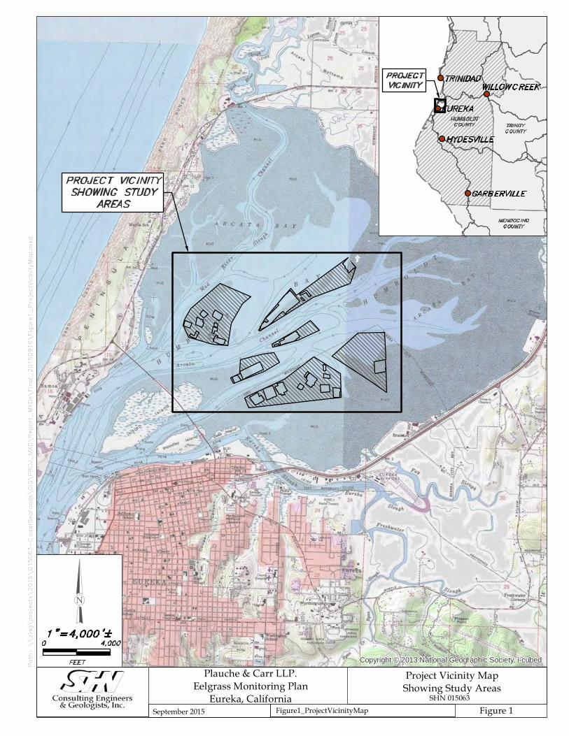
1.0 Introduction This eelgrass monitoring plan was developed by SHN Engineers & Geologists to monitor the effects of Coast Seafoods Company's (Coast) Humboldt Bay Shellfish Culture: Permit Renewal and Expansion Project (Project). As part of the Project and the study area of this monitoring plan (Figure 1), Coast is planning to permit an additional 622 acres of intertidal shellfish aquaculture on historically cultivated shellfish beds (expansion area). Eelgrass is designated as a “Habitat Area of Particular Concern” for federally managed salmonid and groundfish species (NOAA, 2014). Eelgrass beds are also recognized as a conservation concern by local and state agencies, including the California Department of Fish and Wildlife, California Coastal Commission, City of Eureka, and the Humboldt Bay Harbor, Recreation and Conservation District.
1.1 Purpose
This monitoring plan is designed to quantify aquaculture-induced changes in eelgrass percent cover, shoot density, and areal extent within the Project's expansion area. Monitoring is proposed using flyover photography in addition to a before/after-control/impact (BACI) experimental design that includes two years of baseline data (before) and two years of post-project implementation data (after). Nested plots with the two shellfish cultivation methods proposed to take place in eelgrass (cultch-on-longline and basket-on-longline) will be compared to control plots in a blocked design. Monitoring results will be used to evaluate project-related impacts to eelgrass habitat function.
1.2 Project Description The Project has three components:
1) renewing regulatory approvals for 294.5 acres of existing shellfish culture,
2) increasing shellfish culture within an already permitted FLUPSY by adding eight culture bins, and
3) adding an additional 622 acres of intertidal shellfish culture within the expansion area. Two cultivation methods are proposed for intertidal expansion areas where eelgrass occurs: cultch-on-longline and basket-on-longline.1 Cultch-on-longline is proposed to occupy 522 acres within the expansion areas, of which 504 acres occurs in eelgrass habitat. Cultch-on-longline areas will have 100-foot lines spaced 5 feet apart. Basket-on-longline is proposed to occur on approximately 96 acres of eelgrass habitat within the expansion areas. Basket-on-longline areas will have three groups of 100-foot lines spaced 5 feet apart with 20-foot gaps between groups of three lines.
2.0 Regulatory Setting This monitoring plan has been developed in conformance with the California Eelgrass Mitigation Policy and Implementing Guidelines (CEMP) (NOAA, 2014). CEMP recommends compensatory
1 Rack-and-bag cultivation is proposed to occur in a maximum of 4 acres of the expansion area and will not
be placed within 10 feet of existing eelgrass beds.
Copyright:© 2013 National Geographic Society, i-cubedPath: \\
zing\projects\2
015\
015063-C
oastSeafoods\G
IS\P
ROJ_MX
D\Report_
MXDs\Fina
l_20150916\Figu
re1_
ProjectVicinityMap.mxd
Project Vicinity MapShowing Study Areas
SHN 015063Figure 1Figure1_ProjectVicinityMapSeptember 2015
EUREKA
TRINIDAD
HYDESVILLE
GARBERVILLE
WILLOW CREEKPROJECTVICINITY
1 " = 4,000 '±0 4,000
FEET
PROJECT VICINITYSHOWING STUDY
AREAS
HUMBOLDTCOUNTY TRINITY
COUNTY
MENDOCINOCOUNTY
Plauche & Carr LLP.Eelgrass Monitoring Plan
Eureka, California

\\Eureka\Projects\2015\015063-CoastSeafoods\PUBS\Rpts\20150930-EelgrassMonitoringPlan.docx
2
mitigation on an equivalent area basis for loss of spatial cover or statistically significant reductions in eelgrass turion (shoot) density greater than 25 percent. This monitoring plan is designed to assess project-related changes in the percent cover and shoot density eelgrass parameters described in CEMP.
3.0 Location Setting/Characterization Humboldt Bay is a shallow, multi-basin, coastal lagoon with limited freshwater input. Its surface area spans 66 square kilometers at high tide, at least half of which drains during low tides, revealing shallow mudflats connected by subtidal channels. The region has mixed semi-diurnal tides that range in excess of +2.5 meters (m) above mean lower low water (MLLW) to below -0.6 m. Arcata Bay (North Bay) is the northern portion of Humboldt Bay and is the primary location for intertidal shellfish aquaculture. North Bay supports several unique habitat types in addition to an aquaculture industry. In 2009, Humboldt Bay contained 3,614 acres of continuous eelgrass beds and an additional 2,031 acres of patchy eelgrass beds (Schlosser and Eicher, 2012). Although monitoring is sporadic for various locations throughout California, the eelgrass in Humboldt Bay represents up to 53% of California’s eelgrass resource. A variety of environmental factors limit eelgrass growth in the bay, including light and suspended sediments, wind and wave exposure, nutrients, sea surface temperature, space competition, and herbivory.
3.1 Location of Expansion Areas Coast proposes to expand its existing commercial shellfish aquaculture operation in six intertidal areas in North Bay (See Figure 2 and Tables 1 and 2).1
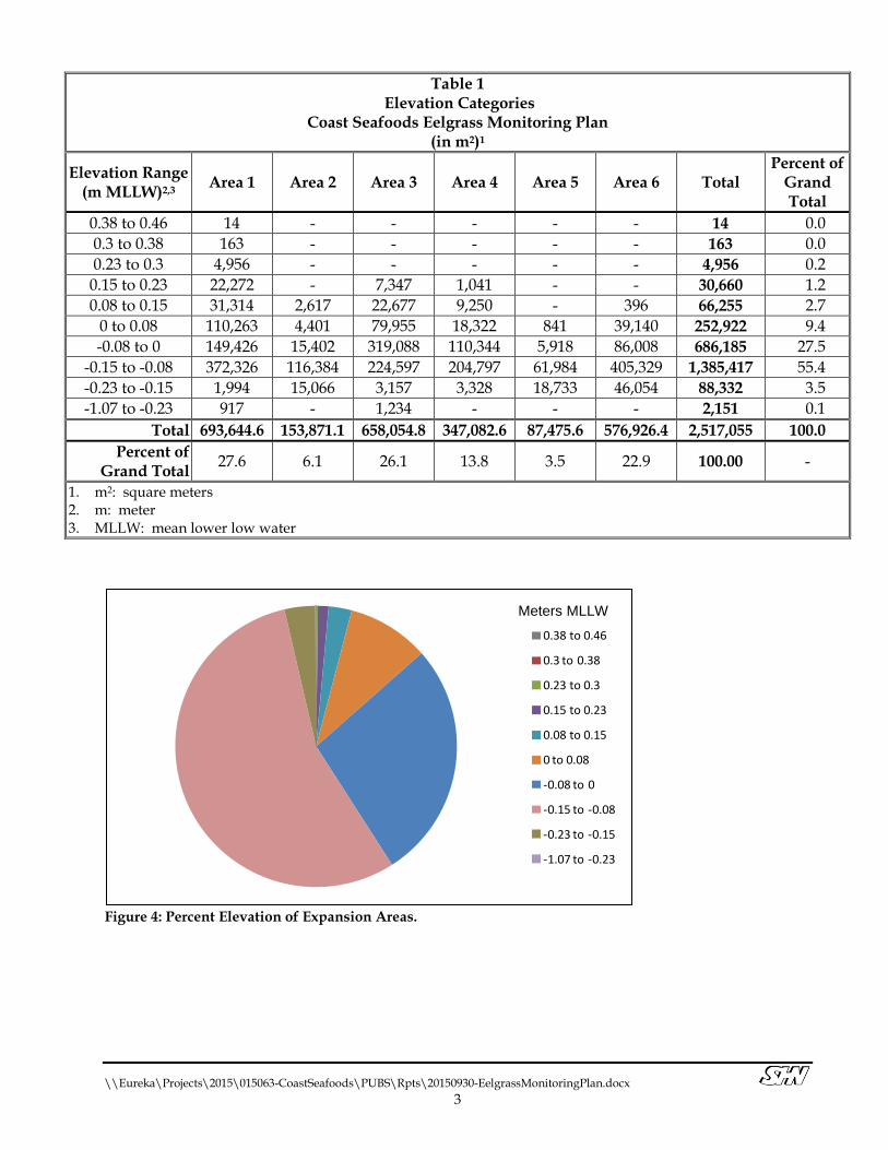
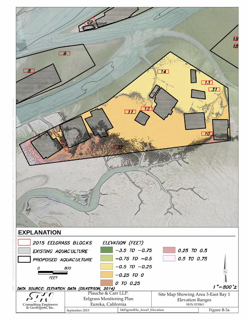
3.2 Elevation As shown in Figures 3 and 4, and presented in Table 1, the expansion area ranges in elevation from -1.07 m MLLW to +0.46 m MLLW (Gilkerson, 2014).

Path: \\
zing\projects\2
015\
015063-C
oastSeafoods\G
IS\P
ROJ_MX
D\Report_
MXDs\Fina
l_20150916\Figu
re2_
StudyAreas.mxd
Site Map ShowingExisting and Expansion Areas
SHN 015063Figure 2Figure2_StudyAreasSeptember 2015
Plauche & Carr LLP.Eelgrass Monitoring Plan
Eureka, California
EXPLANATIONEXISTING AQUACULTUREPROPOSED AQUACULTURE
1 " = 2,000 '±
0 2,000
FEET
AREA 1BIRD ISLAND
AREA 4SAND ISLAND
AREA 5ARCATA CHANNEL
AREA 6EAST BAY 2
AREA 3EAST BAY 1
AREA 2INDIAN ISLAND
DATA SOURCE: AIR PHOTO (NOAA, 2009)

Path: \\
zing\projects\2
015\
015063-C
oastSeafoods\G
IS\P
ROJ_MX
D\Report_
MXDs\Fina
l_20150916\Figu
re3_
ElevationM
ap.mxd
Site Map Showing 1-Foot Elevations andExisting and Expansion Areas
SHN 015063Figure 3Figure3_ElevationMapSeptember 2015
Plauche & Carr LLP.Eelgrass Monitoring Plan
Eureka, California
1 " = 2,000 '±0 2,000
FEET
ELEVATION (FEET)-11 TO -10-10 TO -9-9 TO -8-8 TO -7-7 TO -6-6 TO -5
-5 TO -4-4 TO -3-3 TO -2-2 TO -1-1 TO 00 TO 1
1 TO 22 TO 33 TO 44 TO 55 TO 66 TO 7
DATA SOURCE: ELEVATION DATA (GILKERSON, 2014)
EXPLANATIONEXISTING AQUACULTUREPROPOSED AQUACULTURE
\\Eureka\Projects\2015\015063-CoastSeafoods\PUBS\Rpts\20150930-EelgrassMonitoringPlan.docx
3
Table 1 Elevation Categories
Coast Seafoods Eelgrass Monitoring Plan (in m2)1
Elevation Range (m MLLW)2,3
Area 1 Area 2 Area 3 Area 4 Area 5 Area 6 Total Percent of
Grand Total
0.38 to 0.46 14 - - - - - 14 0.0
0.3 to 0.38 163 - - - - - 163 0.0
0.23 to 0.3 4,956 - - - - - 4,956 0.2
0.15 to 0.23 22,272 - 7,347 1,041 - - 30,660 1.2
0.08 to 0.15 31,314 2,617 22,677 9,250 - 396 66,255 2.7
0 to 0.08 110,263 4,401 79,955 18,322 841 39,140 252,922 9.4
-0.08 to 0 149,426 15,402 319,088 110,344 5,918 86,008 686,185 27.5
-0.15 to -0.08 372,326 116,384 224,597 204,797 61,984 405,329 1,385,417 55.4
-0.23 to -0.15 1,994 15,066 3,157 3,328 18,733 46,054 88,332 3.5
-1.07 to -0.23 917 - 1,234 - - - 2,151 0.1
Total 693,644.6 153,871.1 658,054.8 347,082.6 87,475.6 576,926.4 2,517,055 100.0
Percent of Grand Total
27.6 6.1 26.1 13.8 3.5 22.9 100.00 -
1. m2: square meters 2. m: meter 3. MLLW: mean lower low water
Figure 4: Percent Elevation of Expansion Areas.
0.38 to 0.46
0.3 to 0.38
0.23 to 0.3
0.15 to 0.23
0.08 to 0.15
0 to 0.08
-0.08 to 0
-0.15 to -0.08
-0.23 to -0.15
-1.07 to -0.23
Meters MLLWMeters MLLW
\\Eureka\Projects\2015\015063-CoastSeafoods\PUBS\Rpts\20150930-EelgrassMonitoringPlan.docx
4
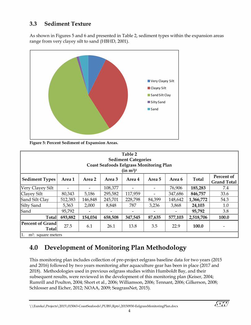
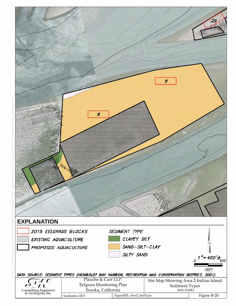
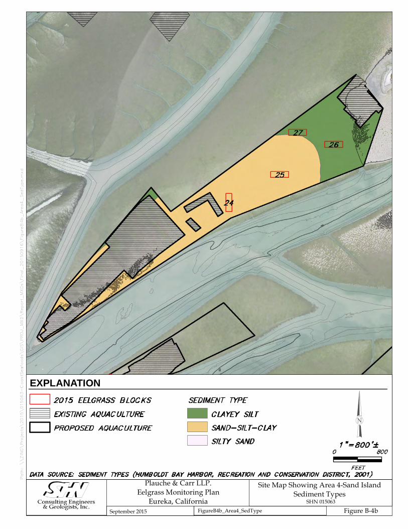
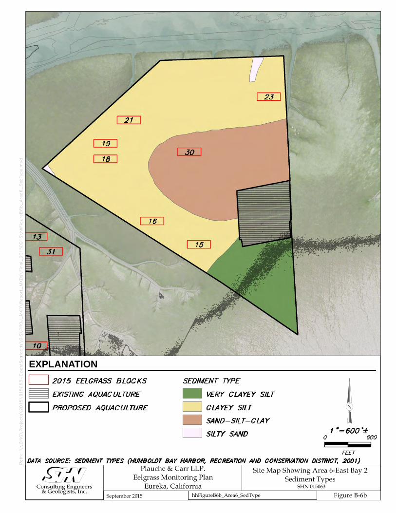
3.3 Sediment Texture As shown in Figures 5 and 6 and presented in Table 2, sediment types within the expansion areas range from very clayey silt to sand (HBHD, 2001).
Figure 5: Percent Sediment of Expansion Areas.
Table 2 Sediment Categories
Coast Seafoods Eelgrass Monitoring Plan (in m2)1
Sediment Types Area 1 Area 2 Area 3 Area 4 Area 5 Area 6 Total Percent of
Grand Total
Very Clayey Silt - - 108,377 - - 76,906 185,283 7.4
Clayey Silt 80,343 5,186 295,582 117,959 - 347,686 846,757 33.6
Sand Silt Clay 512,383 146,848 245,701 228,798 84,399 148,642 1,366,772 54.3
Silty Sand 5,363 2,000 8,848 787 3,236 3,868 24,103 1.0
Sand 95,792 - - - - - 95,792 3.8
Total 693,882 154,034 658,508 347,545 87,635 577,103 2,518,706 100.0
Percent of Grand Total
27.5 6.1 26.1 13.8 3.5 22.9 100.0 -
1. m2: square meters
4.0 Development of Monitoring Plan Methodology This monitoring plan includes collection of pre-project eelgrass baseline data for two years (2015 and 2016) followed by two years monitoring after aquaculture gear has been in place (2017 and 2018). Methodologies used in previous eelgrass studies within Humboldt Bay, and their subsequent results, were reviewed in the development of this monitoring plan (Keiser, 2004; Rumrill and Poulton, 2004; Short et al., 2006; Williamson, 2006; Tennant, 2006; Gilkerson, 2008; Schlosser and Eicher, 2012; NOAA, 2009; SeagrassNet, 2015).
Very Clayey Silt
Clayey Silt
Sand Silt Clay
Silty Sand
Sand

Path: \\
zing\projects\2
015\
015063-C
oastSeafoods\G
IS\P
ROJ_MX
D\Report_
MXDs\Fina
l_20150916\Figu
re6_
Sedim
entTypes.mxd
Site Map Showing Sediment Types andExisting and Expansion Areas
SHN 015063Figure 6Figure6_SedimentTypesSeptember 2015
Plauche & Carr LLP.Eelgrass Monitoring Plan
Eureka, California
1 " = 2,000 '±0 2,000
FEET
EXPLANATIONSEDIMENT TYPES
MARSHSILTY CLAYVERY CLAYEY SILTCLAYEY SILT
SAND-SILT-CLAYSILTY SANDSANDSAND AND GRAVEL
DATA SOURCE: SEDIMENT TYPES (HUMBOLDT BAY HARBOR, RECREATION AND CONSERVATION DISTRICT, 2001)
EXISTING AQUACULTUREPROPOSED AQUACULTURE
\\Eureka\Projects\2015\015063-CoastSeafoods\PUBS\Rpts\20150930-EelgrassMonitoringPlan.docx
5
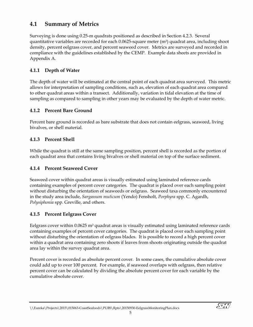
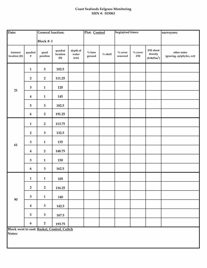
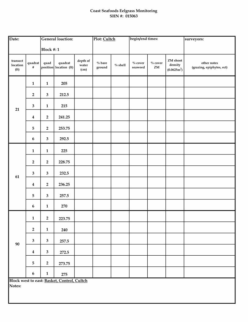
4.1 Summary of Metrics Surveying is done using 0.25-m quadrats positioned as described in Section 4.2.3. Several quantitative variables are recorded for each 0.0625-square meter (m2) quadrat area, including shoot density, percent eelgrass cover, and percent seaweed cover. Metrics are surveyed and recorded in compliance with the guidelines established by the CEMP. Example data sheets are provided in Appendix A.
4.1.1 Depth of Water The depth of water will be estimated at the central point of each quadrat area surveyed. This metric allows for interpretation of sampling conditions, such as, elevation of each quadrat area compared to other quadrat areas within a transect. Additionally, variation in tidal elevation at the time of sampling as compared to sampling in other years may be evaluated by the depth of water metric.
4.1.2 Percent Bare Ground Percent bare ground is recorded as bare substrate that does not contain eelgrass, seaweed, living bivalves, or shell material.
4.1.3 Percent Shell While the quadrat is still at the same sampling position, percent shell is recorded as the portion of each quadrat area that contains living bivalves or shell material on top of the surface sediment.
4.1.4 Percent Seaweed Cover Seaweed cover within quadrat areas is visually estimated using laminated reference cards containing examples of percent cover categories. The quadrat is placed over each sampling point without disturbing the orientation of seaweeds or eelgrass. Seaweed taxa commonly encountered in the study area include, Sargassum muticum (Yendo) Fensholt, Porphyra spp. C. Agardh, Polysiphonia spp. Greville, and others.
4.1.5 Percent Eelgrass Cover Eelgrass cover within 0.0625 m2 quadrat areas is visually estimated using laminated reference cards containing examples of percent cover categories. The quadrat is placed over each sampling point without disturbing the orientation of eelgrass blades. It is possible to record a high percent cover within a quadrat area containing zero shoots if leaves from shoots originating outside the quadrat area lay within the survey quadrat area. Percent cover is recorded as absolute percent cover. In some cases, the cumulative absolute cover could add up to over 100 percent. For example, if seaweed overlaps with eelgrass, then relative percent cover can be calculated by dividing the absolute percent cover for each variable by the cumulative absolute cover.
\\Eureka\Projects\2015\015063-CoastSeafoods\PUBS\Rpts\20150930-EelgrassMonitoringPlan.docx
6
4.1.6 Shoot (Turion) Density After recording percent cover, eelgrass turion density is counted by hand within the 0.0625-m2 quadrat areas (Short et al., 2006). Data will be presented as shoots per m2.
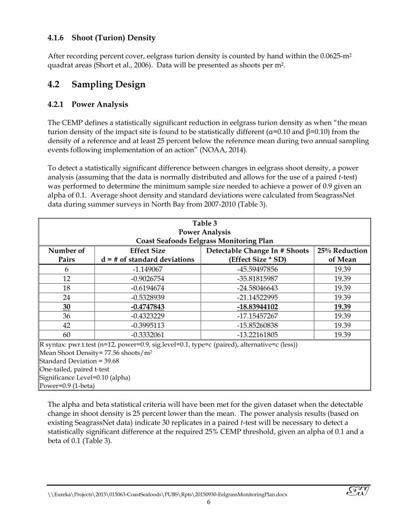
4.2 Sampling Design 4.2.1 Power Analysis The CEMP defines a statistically significant reduction in eelgrass turion density as when “the mean turion density of the impact site is found to be statistically different (α=0.10 and β=0.10) from the density of a reference and at least 25 percent below the reference mean during two annual sampling events following implementation of an action” (NOAA, 2014). To detect a statistically significant difference between changes in eelgrass shoot density, a power analysis (assuming that the data is normally distributed and allows for the use of a paired t-test) was performed to determine the minimum sample size needed to achieve a power of 0.9 given an alpha of 0.1. Average shoot density and standard deviations were calculated from SeagrassNet data during summer surveys in North Bay from 2007-2010 (Table 3).
Table 3 Power Analysis
Coast Seafoods Eelgrass Monitoring Plan
Number of Pairs
Effect Size d = # of standard deviations
Detectable Change In # Shoots (Effect Size * SD)
25% Reduction of Mean
6 -1.149067 -45.59497856 19.39
12 -0.9026754 -35.81815987 19.39
18 -0.6194674 -24.58046643 19.39
24 -0.5328939 -21.14522995 19.39
30 -0.4747843 -18.83944102 19.39
36 -0.4323229 -17.15457267 19.39
42 -0.3995113 -15.85260838 19.39
60 -0.3332061 -13.22161805 19.39
R syntax: pwr.t.test (n=12, power=0.9, sig.level=0.1, type=c (paired), alternative=c (less)) Mean Shoot Density= 77.56 shoots/m2 Standard Deviation = 39.68 One-tailed, paired t-test Significance Level=0.10 (alpha) Power=0.9 (1-beta)
The alpha and beta statistical criteria will have been met for the given dataset when the detectable change in shoot density is 25 percent lower than the mean. The power analysis results (based on existing SeagrassNet data) indicate 30 replicates in a paired t-test will be necessary to detect a statistically significant difference at the required 25% CEMP threshold, given an alpha of 0.1 and a beta of 0.1 (Table 3).
\\Eureka\Projects\2015\015063-CoastSeafoods\PUBS\Rpts\20150930-EelgrassMonitoringPlan.docx
7
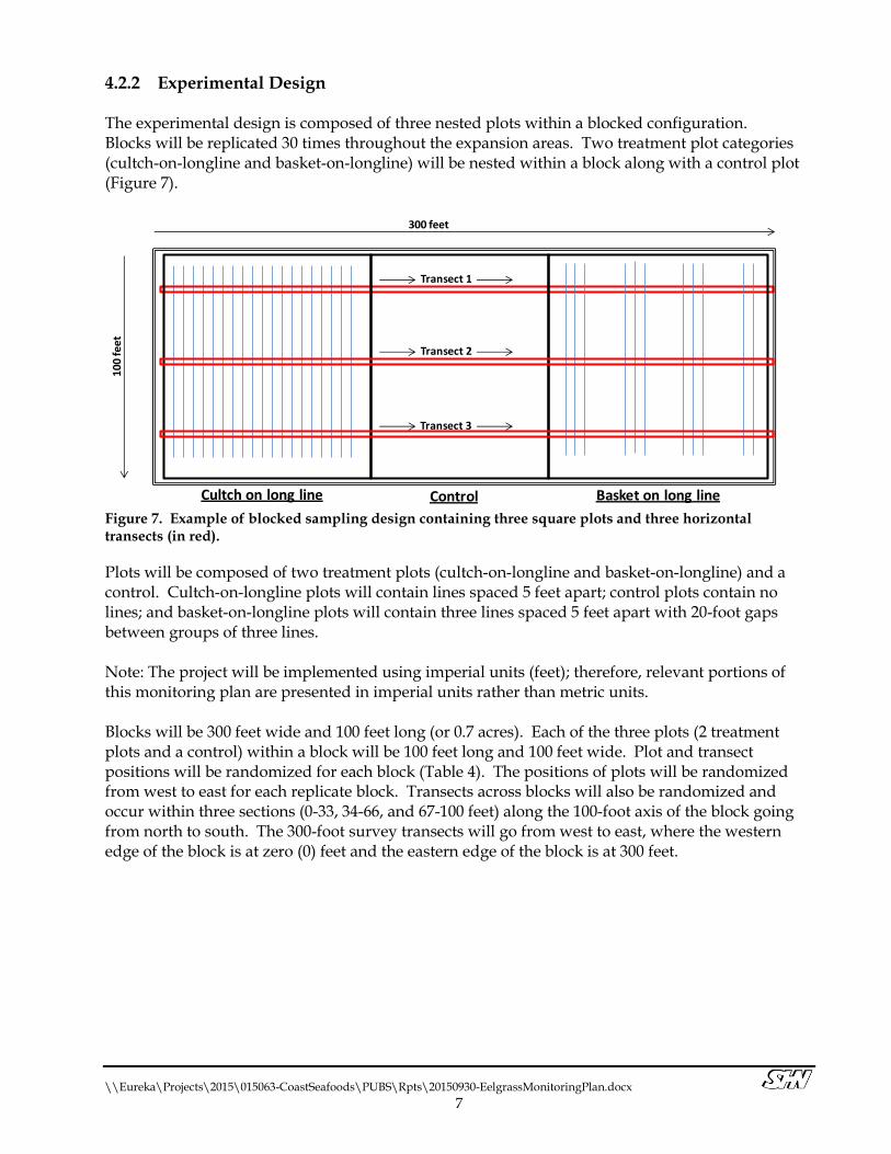
4.2.2 Experimental Design The experimental design is composed of three nested plots within a blocked configuration. Blocks will be replicated 30 times throughout the expansion areas. Two treatment plot categories (cultch-on-longline and basket-on-longline) will be nested within a block along with a control plot (Figure 7).
Figure 7. Example of blocked sampling design containing three square plots and three horizontal transects (in red).
Plots will be composed of two treatment plots (cultch-on-longline and basket-on-longline) and a control. Cultch-on-longline plots will contain lines spaced 5 feet apart; control plots contain no lines; and basket-on-longline plots will contain three lines spaced 5 feet apart with 20-foot gaps between groups of three lines. Note: The project will be implemented using imperial units (feet); therefore, relevant portions of this monitoring plan are presented in imperial units rather than metric units. Blocks will be 300 feet wide and 100 feet long (or 0.7 acres). Each of the three plots (2 treatment plots and a control) within a block will be 100 feet long and 100 feet wide. Plot and transect positions will be randomized for each block (Table 4). The positions of plots will be randomized from west to east for each replicate block. Transects across blocks will also be randomized and occur within three sections (0-33, 34-66, and 67-100 feet) along the 100-foot axis of the block going from north to south. The 300-foot survey transects will go from west to east, where the western edge of the block is at zero (0) feet and the eastern edge of the block is at 300 feet.
300 feet
100
fee
t
Transect 1
Transect 2
Transect 3
Cultch on long line Control Basket on long line
\\Eureka\Projects\2015\015063-CoastSeafoods\PUBS\Rpts\20150930-EelgrassMonitoringPlan.docx
8
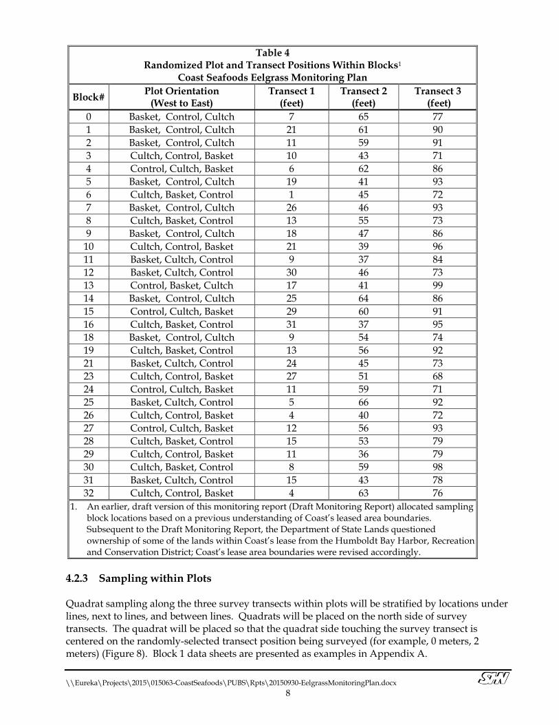
Table 4
Randomized Plot and Transect Positions Within Blocks1 Coast Seafoods Eelgrass Monitoring Plan
Block# Plot Orientation
(West to East) Transect 1
(feet) Transect 2
(feet) Transect 3
(feet)
0 Basket, Control, Cultch 7 65 77 1 Basket, Control, Cultch 21 61 90 2 Basket, Control, Cultch 11 59 91 3 Cultch, Control, Basket 10 43 71 4 Control, Cultch, Basket 6 62 86 5 Basket, Control, Cultch 19 41 93 6 Cultch, Basket, Control 1 45 72 7 Basket, Control, Cultch 26 46 93 8 Cultch, Basket, Control 13 55 73 9 Basket, Control, Cultch 18 47 86
10 Cultch, Control, Basket 21 39 96 11 Basket, Cultch, Control 9 37 84 12 Basket, Cultch, Control 30 46 73 13 Control, Basket, Cultch 17 41 99 14 Basket, Control, Cultch 25 64 86 15 Control, Cultch, Basket 29 60 91 16 Cultch, Basket, Control 31 37 95 18 Basket, Control, Cultch 9 54 74 19 Cultch, Basket, Control 13 56 92 21 Basket, Cultch, Control 24 45 73 23 Cultch, Control, Basket 27 51 68 24 Control, Cultch, Basket 11 59 71 25 Basket, Cultch, Control 5 66 92 26 Cultch, Control, Basket 4 40 72 27 Control, Cultch, Basket 12 56 93 28 Cultch, Basket, Control 15 53 79 29 Cultch, Control, Basket 11 36 79 30 Cultch, Basket, Control 8 59 98 31 Basket, Cultch, Control 15 43 78 32 Cultch, Control, Basket 4 63 76
1. An earlier, draft version of this monitoring report (Draft Monitoring Report) allocated sampling block locations based on a previous understanding of Coast’s leased area boundaries. Subsequent to the Draft Monitoring Report, the Department of State Lands questioned ownership of some of the lands within Coast’s lease from the Humboldt Bay Harbor, Recreation and Conservation District; Coast’s lease area boundaries were revised accordingly.
4.2.3 Sampling within Plots
Quadrat sampling along the three survey transects within plots will be stratified by locations under lines, next to lines, and between lines. Quadrats will be placed on the north side of survey transects. The quadrat will be placed so that the quadrat side touching the survey transect is centered on the randomly-selected transect position being surveyed (for example, 0 meters, 2 meters) (Figure 8). Block 1 data sheets are presented as examples in Appendix A.
\\Eureka\Projects\2015\015063-CoastSeafoods\PUBS\Rpts\20150930-EelgrassMonitoringPlan.docx
9
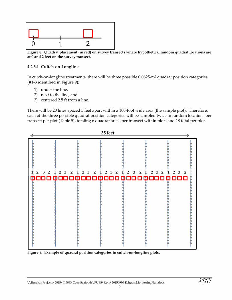
Figure 8. Quadrat placement (in red) on survey transects where hypothetical random quadrat locations are at 0 and 2 feet on the survey transect.
4.2.3.1 Cultch-on-Longline In cutch-on-longline treatments, there will be three possible 0.0625-m2 quadrat position categories (#1-3 identified in Figure 9):
1) under the line, 2) next to the line, and 3) centered 2.5 ft from a line.
There will be 20 lines spaced 5 feet apart within a 100-foot wide area (the sample plot). Therefore, each of the three possible quadrat position categories will be sampled twice in random locations per transect per plot (Table 5), totaling 6 quadrat areas per transect within plots and 18 total per plot.
Figure 9. Example of quadrat position categories in cultch-on-longline plots.
0 1 2
35 feet
1 2 3 2 1 2 3 2 1 2 3 2 1 2 3 2 1 2 3 2 1 2 3 2 1 2 3 2
\\Eureka\Projects\2015\015063-CoastSeafoods\PUBS\Rpts\20150930-EelgrassMonitoringPlan.docx
10
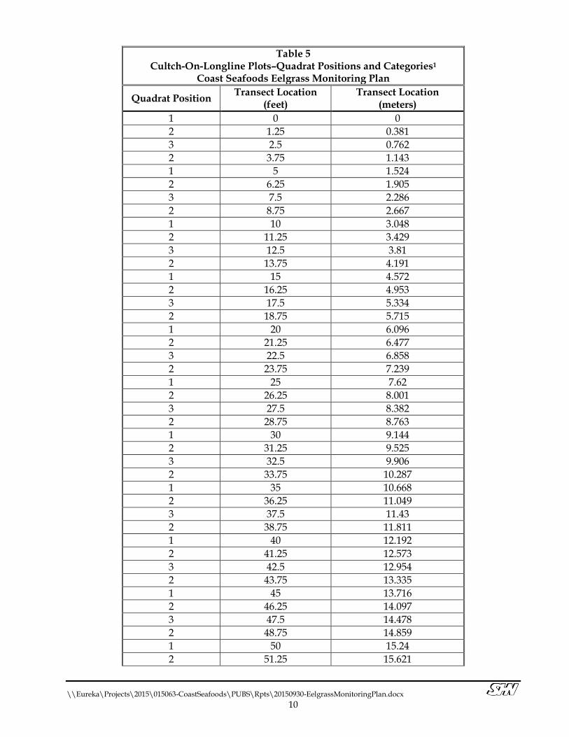
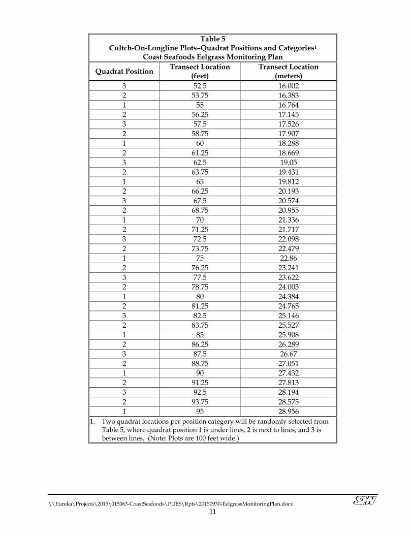
Table 52 Cultch-On-Longline Plots–Quadrat Positions and Categories1
Coast Seafoods Eelgrass Monitoring Plan
Quadrat Position Transect Location
(feet) Transect Location
(meters)
1 0 0
2 1.25 0.381
3 2.5 0.762
2 3.75 1.143
1 5 1.524
2 6.25 1.905
3 7.5 2.286
2 8.75 2.667
1 10 3.048
2 11.25 3.429
3 12.5 3.81
2 13.75 4.191
1 15 4.572
2 16.25 4.953
3 17.5 5.334
2 18.75 5.715
1 20 6.096
2 21.25 6.477
3 22.5 6.858
2 23.75 7.239
1 25 7.62
2 26.25 8.001
3 27.5 8.382
2 28.75 8.763
1 30 9.144
2 31.25 9.525
3 32.5 9.906
2 33.75 10.287
1 35 10.668
2 36.25 11.049
3 37.5 11.43
2 38.75 11.811
1 40 12.192
2 41.25 12.573
3 42.5 12.954
2 43.75 13.335
1 45 13.716
2 46.25 14.097
3 47.5 14.478
2 48.75 14.859
1 50 15.24
2 51.25 15.621
\\Eureka\Projects\2015\015063-CoastSeafoods\PUBS\Rpts\20150930-EelgrassMonitoringPlan.docx
11
Table 52 Cultch-On-Longline Plots–Quadrat Positions and Categories1
Coast Seafoods Eelgrass Monitoring Plan
Quadrat Position Transect Location
(feet) Transect Location
(meters)
3 52.5 16.002
2 53.75 16.383
1 55 16.764
2 56.25 17.145
3 57.5 17.526
2 58.75 17.907
1 60 18.288
2 61.25 18.669
3 62.5 19.05
2 63.75 19.431
1 65 19.812
2 66.25 20.193
3 67.5 20.574
2 68.75 20.955
1 70 21.336
2 71.25 21.717
3 72.5 22.098
2 73.75 22.479
1 75 22.86
2 76.25 23.241
3 77.5 23.622
2 78.75 24.003
1 80 24.384
2 81.25 24.765
3 82.5 25.146
2 83.75 25.527
1 85 25.908
2 86.25 26.289
3 87.5 26.67
2 88.75 27.051
1 90 27.432
2 91.25 27.813
3 92.5 28.194
2 93.75 28.575
1 95 28.956
1. Two quadrat locations per position category will be randomly selected from Table 5, where quadrat position 1 is under lines, 2 is next to lines, and 3 is between lines. (Note: Plots are 100 feet wide.)

\\Eureka\Projects\2015\015063-CoastSeafoods\PUBS\Rpts\20150930-EelgrassMonitoringPlan.docx
12
4.2.3.2 Basket-on-Longline In basket-on-longline treatments, there will be four possible 0.0625-m2 quadrat position categories (#1-4 identified in Figure 10):
1) under the line, 2) next to the line, 3) 5 feet from the closest line in 20-foot gaps, and 4) 10 feet from the closest line in 20-foot gaps.
Within a 100-foot wide area (same sample plot) there will be groups of 3 lines spaced 5 feet apart with 20-foot gaps between groups lines (see Figure 10, below). Therefore, each of the four possible quadrat positions will be sampled twice in random locations per transect (Table 6), totaling 8 quadrat areas per transect and 24 per plot.
Figure 10. Example of quadrat position categories in basket-on-longline plots.
100 feet
1 2 1 2 1 3 4 3 1 2 1 2 1 3 4 3 1 2 1 2 1 3 4 3 1 2 1

\\Eureka\Projects\2015\015063-CoastSeafoods\PUBS\Rpts\20150930-EelgrassMonitoringPlan.docx
13
Table 6 Basket-On-Longline Plots–Quadrat Positions and Categories1
Coast Seafoods Eelgrass Monitoring Plan
Quadrat Position Transect Location
(feet) Transect Location
(meters)
1 0 0
2 2.5 0.762
1 5 1.524
2 7.5 2.286
1 10 3.048
3 15 4.572
4 20 6.096
3 25 7.62
1 30 9.144
2 32.5 9.906
1 35 10.668
2 37.5 11.43
1 40 12.192
3 45 13.716
4 50 15.24
3 55 16.764
1 60 18.288
2 62.5 19.05
1 65 19.812
2 67.5 20.574
1 70 21.336
3 75 22.86
4 80 24.384
3 85 25.908
1 90 27.432
2 92.5 28.194
1 95 28.956
1. Two quadrat locations per position category will be selected from Table 6, where quadrat position 1 is under lines, 2 is between lines spaced 5 feet apart, 3 is next to lines spaced 20 feet apart, and 4 is between lines spaced 20 feet apart.
4.2.4 Control Because the control plots will not have longlines, the quadrat position spacing for cultch-on-longline plots will be used within control plots without designations pertaining to positions under, next to, or between lines.
\\Eureka\Projects\2015\015063-CoastSeafoods\PUBS\Rpts\20150930-EelgrassMonitoringPlan.docx
14
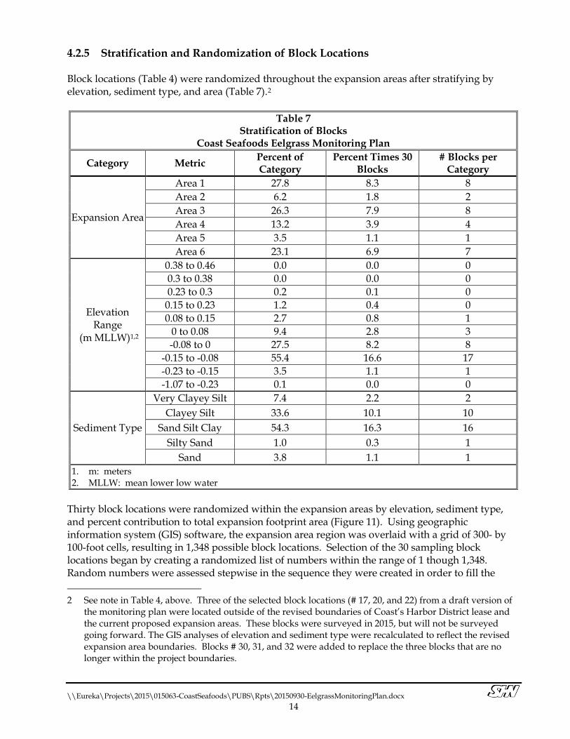
4.2.5 Stratification and Randomization of Block Locations Block locations (Table 4) were randomized throughout the expansion areas after stratifying by elevation, sediment type, and area (Table 7).4F
2
Table 7 Stratification of Blocks
Coast Seafoods Eelgrass Monitoring Plan
Category Metric Percent of Category
Percent Times 30 Blocks
# Blocks per Category
Expansion Area
Area 1 27.8 8.3 8
Area 2 6.2 1.8 2
Area 3 26.3 7.9 8
Area 4 13.2 3.9 4
Area 5 3.5 1.1 1
Area 6 23.1 6.9 7
Elevation Range
(m MLLW)1,2
0.38 to 0.46 0.0 0.0 0
0.3 to 0.38 0.0 0.0 0
0.23 to 0.3 0.2 0.1 0
0.15 to 0.23 1.2 0.4 0
0.08 to 0.15 2.7 0.8 1
0 to 0.08 9.4 2.8 3
-0.08 to 0 27.5 8.2 8
-0.15 to -0.08 55.4 16.6 17
-0.23 to -0.15 3.5 1.1 1
-1.07 to -0.23 0.1 0.0 0
Sediment Type
Very Clayey Silt 7.4 2.2 2
Clayey Silt 33.6 10.1 10
Sand Silt Clay 54.3 16.3 16
Silty Sand 1.0 0.3 1
Sand 3.8 1.1 1
1. m: meters 2. MLLW: mean lower low water
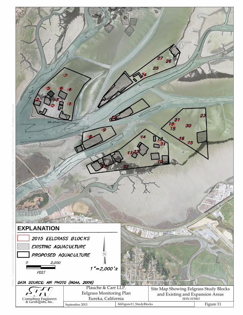
Thirty block locations were randomized within the expansion areas by elevation, sediment type, and percent contribution to total expansion footprint area (Figure 11). Using geographic information system (GIS) software, the expansion area region was overlaid with a grid of 300- by 100-foot cells, resulting in 1,348 possible block locations. Selection of the 30 sampling block locations began by creating a randomized list of numbers within the range of 1 though 1,348. Random numbers were assessed stepwise in the sequence they were created in order to fill the
2 See note in Table 4, above. Three of the selected block locations (# 17, 20, and 22) from a draft version of
the monitoring plan were located outside of the revised boundaries of Coast’s Harbor District lease and the current proposed expansion areas. These blocks were surveyed in 2015, but will not be surveyed going forward. The GIS analyses of elevation and sediment type were recalculated to reflect the revised expansion area boundaries. Blocks # 30, 31, and 32 were added to replace the three blocks that are no longer within the project boundaries.
18
6
0
5
2
9
3
7
4
1
8
28
29
3116
26
3023
2527
1314
32
2119
1511
24
1210
Path: \\
zing\projects\2
015\
015063-C
oastSeafoods\G
IS\P
ROJ_MX
D\Report_
MXDs\Fina
l_20150916\hhFigu
re11_S
tudyBlocks.mxd
Site Map Showing Eelgrass Study Blocksand Existing and Expansion Areas
SHN 015063Figure 11hhFigure11_StudyBlocksSeptember 2015
Plauche & Carr LLP.Eelgrass Monitoring Plan
Eureka, California
1 " = 2,000 '±0 2,000
FEET
EXPLANATION2015 EELGRASS BLOCKSEXISTING AQUACULTUREPROPOSED AQUACULTURE
DATA SOURCE: AIR PHOTO (NOAA, 2009)

\\Eureka\Projects\2015\015063-CoastSeafoods\PUBS\Rpts\20150930-EelgrassMonitoringPlan.docx
15
allocated number of blocks per category. If a number in the selection process occurred in a category that was already filled, that number was discarded and the next number was evaluated to fill a category. If the majority of a randomly selected block location was out of the expansion area or overlapping with existing aquaculture, that block was also discarded. In a few instances, where obstructions such as minor sloughs or other edge effects occurred, randomly selected block locations were adjusted to the closest possible configuration. Detailed block locations are shown in Appendix B.
4.3 Statistical Analysis Summary statistics for percent eelgrass cover and shoot density within plots will include the average, standard deviation, and sample size. After completion of the second year of surveying post impact, a paired t-test will be run comparing the average shoot density per plot before impact and after impact, after adjusting before impact data if there are reductions in shoot density in the control plots (NOAA, 2014). If the data does not appear to be normally distributed, then other statistical methods will be used (for example, multivariate) to analyze the data. A more detailed description of calculations used to estimate shoot density at the plot level; percent differences in mean shoot density between treatment and control plots; and test statistics to determine whether the difference between treatment and controls changed significantly after project implementation can be found in Appendix C.
4.4 Survey Logistics and Schedule Blocks will be located by global positioning system (GPS) coordinates of block corners. Half-inch polyvinyl chloride (PVC) pipe, approximately 1.5 m long, will be used to mark block corners. Transect tapes measuring 100 feet in length will be deployed from the northern block corners to the southern block corners, so that the north end is at zero (0) feet and the south end is 100 feet. After the 100-foot transect tapes are in place, 300-foot survey transect tapes will be deployed from west to east at the randomly chosen transect locations, so that the west side is at zero (0) feet and the east side is 300 feet. The northwest block corner is the 0,0 location that serves as an anchor point from which all other location adjustments are based after locating GPS block corner locations. Each block will be surveyed by a team of six people. Each plot within a block will be surveyed by two people, where one person records data on datasheets and the other person calls out the data to the scribe. Impacts to soft sediment and eelgrass will be minimized by the use of boogie boards as surfaces on which the surveyors stand and kneel. Sampling will occur on tides predicted to be -0.3 m MLLW or lower during the active growth period for eelgrass in northern California (May-September) (NOAA, 2014) during the years of 2015, 2016, 2017, and 2018.
5.0 Spatial Distribution and Areal Extent of Eelgrass In compliance with the CEMP, this monitoring plan proposes the use of aerial photography to determine the pre- and post-project areal extent and spatial distribution of eelgrass habitat within the project vicinity. The CEMP defines an eelgrass habitat as “areas of vegetated eelgrass cover (any eelgrass within 1 m of another shoot) bounded by a 5 m wide perimeter of unvegetated area.” Therefore, under the CEMP, if there is a reduction in the areal extent (i.e., acreage) of eelgrass

\\Eureka\Projects\2015\015063-CoastSeafoods\PUBS\Rpts\20150930-EelgrassMonitoringPlan.docx
16
habitat that results in a greater than 1-m gap it is considered a significant impact. Areal extent of eelgrass habitat is defined as the quantitative area of the spatial distribution, categorized as vegetated cover or unvegetated habitat. The most recent complete dataset for eelgrass distribution in North Bay was mapped using camera imagery from airplane flyovers (NOAA, 2009). Because high-quality aerial imagery requires minimum sun angles, clear weather and low tides, there were substantial logistical difficulties in obtaining this imagery. The only tides low enough (-0.3 m or lower) to reveal the full extent of eelgrass beds in Humboldt Bay during daylight hours occur in the early mornings between May and August each year. These months coincide with weather conditions that make aerial photography difficult, particularly heavy morning fog when the tide is at its lowest. As a result, it took NOAA three years of attempted flyovers before there was one day when all of the following logistics lined up: a tide of -0.3 m or lower; sky clear from clouds, fog, or haze; a sun angle of 30° or higher; and winds of 10 miles per hour (mph) or less. This monitoring plan recognizes the challenges in mapping eelgrass spatial distribution within the 622 acres of expanded aquaculture. Therefore, this plan recommends a flexible approach in assessing the spatial distribution of eelgrass within the expansion areas. In order to obtain visible light and/or infrared spectrum images during the eelgrass active growth season during the years 2016 (pre-project) and 2017-18 (two years post-project), this plan recommends using either: 1) an airplane with pilot and photographer flown at an approximately 500-m elevation: or 2) a remote controlled airplane/drone flown at an approximately 120-m elevation. The most appropriate method of aerial photography will be selected on any given day based on the status of the above variables.
5.1 Manned Airplane Imagery Collection Imagery from the manned airplane would be combined to create one large composite image of the expansion area vicinity within North Bay. Attempts to orthorectify and georeference the dataset will be made pending the outcome of composite image.
5.2 Remote Controlled Airplane/Drone Imagery Collection Imagery from the remote controlled airplane/drone would be acquired from a camera mounted to the aircraft. All images will contain location coordinates and be post-processed to create one composite image that is orthorectified and georeferenced.
5.3 Mapping Spatial Distribution Spatial distribution will be mapped at a resolution to be determined by the outcome of composite imagery. The 2009 NOAA imagery contains 0.5- x 0.5-m pixels and is the highest resolution imagery publically available for Humboldt Bay. This monitoring plan anticipates a mapping resolution equal to or better than the 2009 NOAA imagery and anticipates that the composite image of the expansion area vicinity will be orthorectified and georeferenced, allowing GIS mapping of vegetated cover and unvegetated habitat. The resolution of this mapping effort will be determined by the resolution of the images obtained.

\\Eureka\Projects\2015\015063-CoastSeafoods\PUBS\Rpts\20150930-EelgrassMonitoringPlan.docx
17
5.4 Calculating Areal Extent Areal extent of vegetated cover and unvegetated habitat will be calculated from the spatial distribution map using GIS software.
5.5 Evaluating Project-Induced Changes in Areal Extent The areal extent of eelgrass within the expansion areas after two years of full project implementation (2018) will be compared to pre-project (2016) conditions. In coordination with regulatory agencies, reference sites outside the influence of aquaculture activities will be selected within the vicinity of the expansion areas and within the area of imagery collected. These reference sites will be used to characterize natural fluctuations in eelgrass areal extent to which potential aquaculture induced impacts can be compared.
6.0 References
Coast Seafoods Company. (January 20, 2015). Draft Initial Study, Coast Seafoods Company, Humboldt Bay Shellfish Culture Permit Renewal and Expansion Project. Available at: http://humboldtbay.org/sites/humboldtbay2.org/files/CoUastU%20Project%20-%20Initial%20Study%20-%20Draft%20-%20Jan%2020%202015.pdf
Gilkerson, W. (2008). A Spatial Model of Eelgrass (Zostera marina) Habitat in Humboldt Bay, California. Master’s Thesis. Arcata CA:HSU.
---. (2014). Humboldt Bay Sea Level Rise DEM Development Report. Arcata, CA:Pacific Watershed Associates, Inc.
Humboldt Bay Harbor, Recreation, and Conservation District. (2001). “Humboldt Bay Sediments Map.” Accessed on April 22, 2015. Available at: http://humboldtbay.org/sites/humboldtbay.org/files/gis_data/sediments.pdf
Keiser, A. L. (2004). A Study of the Spatial and Temporal Variation of Eelgrass, Zostera Marina, its Epiphytes, and the Grazer Phyllaplysia Taylori in Arcata Bay, California, USA. (Master’s thesis, Humboldt State University). Arcata, CA:HSU.
National Geographic Society, i-cubed. (2013). “Map of Humboldt Bay, California.” Accessed at: http://maps.nationalgeographic.com/maps
National Oceanic and Atmospheric Administration. (2009). “Humboldt Bay, California Benthic Habitats.” Charleston, SC:NOAA Coastal Services. Available at: https://data.noaa.gov/dataset/humboldt-bay-california-benthic-habitats-2009
--- . (2014). “California Eelgrass Mitigation Policy and Implementing Guidelines.” (October 2014). NOAA Fisheries West Coast Region. Available at: http://www.westcoUastU.fisheries.noaa.gov/publications/habitat/california_eelgrass_mitigation/Final%20CEMP%20October%202014/cemp_oct_2014_final.pdf
Rumrill, S. S. and V. K. Poulton. (2004). Ecological Role and Potential Impacts of Molluscan Shellfish Culture in the Estuarine Environment of Humboldt Bay, CA. Seattle, WA:US Department of Agriculture, Western Regional Aquaculture Center.
Schlosser, S. and A. Eicher. (2012). The Humboldt Bay and Eel River Estuary Benthic Habitat Project. California Sea Grant Publication T-075. 246 p. La Jolla, CA:California Sea Grant.
\\Eureka\Projects\2015\015063-CoastSeafoods\PUBS\Rpts\20150930-EelgrassMonitoringPlan.docx
18
SeagrassNet. (2015). “Humboldt Bay, California Station CH42.2.” (provided by Adam Wagschal). NR:Global Seagrass Monitoring Network.
Short, F. T., L. J. McKenzie, R. G. Coles, K. P. Vidler, and J. L. Gaeckle. (2006). Seagrassnet Manual for Scientific Monitoring of Seagrass Habitat, Worldwide Edition. Durham, NH:University of New Hampshire Publication.
Tennant, G. (2006). Experimental Effects of Ammonium on Eelgrass (Zostera marina L.) Shoot Density in Humboldt Bay, California (Master’s thesis, Humboldt State University). Arcata, CA:HSU.
Williamson, K. J. (2006). Relationships between Eelgrass (Zostera marina) Habitat Characteristics and Juvenile Dungeness Crab (cancer magister) and Other Invertebrates in Southern Humboldt Bay, California, USA (Master’s thesis, Humboldt State University). Arcata, CA:HSU.

A Exam
ple
Data
Sh
eets

Coast Seafoods Eelgrass MonitoringSHN #: 015063
surveyors:
transectlocation (ft) quadrat # quad
position
quadrat location
(ft)
depth of water (cm)
% bare ground % shell % cover
seaweed% cover
ZM
ZM shoot density
(0.0625m2)
other notes (grazing, epiphytes, ect)
1 2 2.5
2 1 5
3 2 7.5
4 3 25
5 3 45
6 4 50
7 1 60
8 4 80
1 2 7.5
2 4 20
3 1 30
4 1 40
5 4 50
6 2 62.5
7 3 75
8 3 85
1 2 7.5
2 3 15
3 4 20
4 1 60
5 1 65
6 2 67.5
7 4 80
8 3 85Block west to east: Basket, Control, CultchNotes:
21
General loaction:
Block #: 1
Date: Plot: Basket
61
90
begin/end times:
Coast Seafoods Eelgrass MonitoringSHN #: 015063
surveyors:
transectlocation (ft)
quadrat #
quad position
quadrat location
(ft)
depth of water (cm)
% bare ground % shell % cover
seaweed% cover
ZM
ZM shoot density
(0.0625m2)
other notes (grazing, epiphytes, ect)
1 3 102.5
2 2 111.25
3 1 120
4 1 145
5 3 182.5
6 2 191.25
1 2 113.75
2 3 132.5
3 1 135
4 2 148.75
5 1 150
6 3 162.5
1 1 105
2 2 116.25
3 1 140
4 3 142.5
5 3 167.5
6 2 193.75Block west to east: Basket, Control, CultchNotes:
Date: Plot: Control
21
61
90
begin/end times:General loaction:
Block #: 1
Coast Seafoods Eelgrass MonitoringSHN #: 015063
surveyors:
transectlocation
(ft)
quadrat #
quad position
quadrat location (ft)
depth of water (cm)
% bare ground % shell % cover
seaweed% cover
ZM
ZM shoot density
(0.0625m2)
other notes (grazing, epiphytes, ect)
1 1 205
2 3 212.5
3 1 215
4 2 241.25
5 2 253.75
6 3 292.5
1 1 225
2 2 228.75
3 3 232.5
4 2 236.25
5 3 257.5
6 1 270
1 2 223.75
2 1 240
3 3 257.5
4 3 272.5
5 2 273.75
6 1 275Block west to east: Basket, Control, CultchNotes:
Date: Plot: Cultch
21
61
90
begin/end times:General loaction:
Block #: 1
B Blo
ck L
oca
tio
ns
By
Are
a

6
1
4
7
8
2
5
0
3
Path: \\
zing\projects\2
015\
015063-C
oastSeafoods\G
IS\P
ROJ_MX
D\Report_
MXDs\Fina
l_20150916\Figu
reB1
a_Area1_
Elevation.mxd
Site Map Showing Area 1-Bird IslandElevation Ranges
SHN 015063Figure B-1aFigureB1a_Area1_ElevationSeptember 2015
Plauche & Carr LLP.Eelgrass Monitoring Plan
Eureka, California
1 " = 600 '±
0 600
FEET
DATA SOURCE: ELEVATION DATA (GILKERSON, 2014)
EXPLANATIONELEVATION (FEET)2015 EELGRASS BLOCKS
EXISTING AQUACULTUREPROPOSED AQUACULTURE
-3.52 TO -3.50-3.50 TO -0.75-0.75 TO -0.5-0.5 TO -0.25-0.25 TO 0
0 TO 0.250.25 TO 0.50.5 TO 0.750.75 TO 11 TO 1.251.25 TO 1.5

6
1
4
7
8
2
5
0
3
Path: \\
ZING
\Projec
ts\2015\
015063-C
oastSeafoods\G
IS\PROJ_M
XD\R
eport_MX
Ds\Fina
l_20150916\Figu
reB1
b_Area1_
SedType.m
xd
Site Map Showing Area 1-Bird IslandSediment Types
SHN 015063Figure B-1bFigureB1b_Area1_SedTypeSeptember 2015
Plauche & Carr LLP.Eelgrass Monitoring Plan
Eureka, California
1 " = 600 '±0 600
FEETDATA SOURCE: SEDIMENT TYPES (HUMBOLDT BAY HARBOR, RECREATION AND CONSERVATION DISTRICT, 2001)
EXPLANATIONSEDIMENT TYPE
CLAYEY SILTSAND-SILT-CLAYSILTY SANDSAND
2015 EELGRASS BLOCKSEXISTING AQUACULTUREPROPOSED AQUACULTURE
9
8
28
29Path: \\
zing\projects\2
015\
015063-C
oastSeafoods\G
IS\P
ROJ_MX
D\Report_
MXDs\Fina
l_20150916\Figu
reB2
a_Area2_
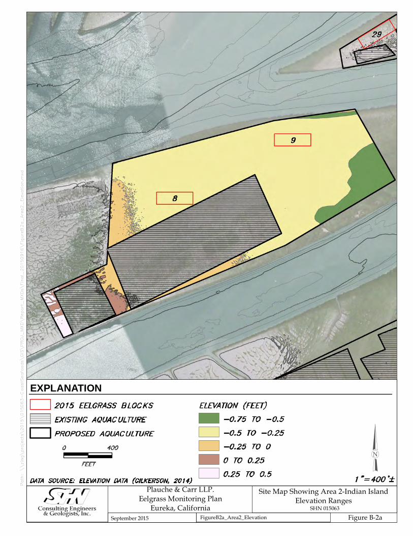
Elevation.mxd
Site Map Showing Area 2-Indian IslandElevation Ranges
SHN 015063Figure B-2aFigureB2a_Area2_ElevationSeptember 2015
Plauche & Carr LLP.Eelgrass Monitoring Plan
Eureka, California
1 " = 400 '±
0 400
FEET
DATA SOURCE: ELEVATION DATA (GILKERSON, 2014)
EXPLANATIONELEVATION (FEET)
-0.75 TO -0.5-0.5 TO -0.25-0.25 TO 00 TO 0.250.25 TO 0.5
2015 EELGRASS BLOCKSEXISTING AQUACULTUREPROPOSED AQUACULTURE
9
8
28
29Path: \\
ZING
\Projec
ts\2015\
015063-C
oastSeafoods\G
IS\PROJ_M
XD\R
eport_MX
Ds\Fina
l_20150916\Figu
reB2
b_Area2_
SedType.m
xd
Site Map Showing Area 2-Indian IslandSediment Types
SHN 015063Figure B-2bFigureB2b_Area2_SedTypeSeptember 2015
Plauche & Carr LLP.Eelgrass Monitoring Plan
Eureka, California
1 " = 400 '±0 400
FEETDATA SOURCE: SEDIMENT TYPES (HUMBOLDT BAY HARBOR, RECREATION AND CONSERVATION DISTRICT, 2001)
EXPLANATIONSEDIMENT TYPE
CLAYEY SILTSAND-SILT-CLAYSILTY SAND
2015 EELGRASS BLOCKSEXISTING AQUACULTUREPROPOSED AQUACULTURE
8
9
28
29
31
32
14
13
11 12
10
1918
Path: \\
zing\projects\2
015\
015063-C
oastSeafoods\G
IS\P
ROJ_MX
D\Report_
MXDs\Fina
l_20150916\hhFigu
reB3
a_Area3_
Elevation.mxd
Site Map Showing Area 3-East Bay 1Elevation Ranges
SHN 015063Figure B-3ahhFigureB3a_Area3_ElevationSeptember 2015
Plauche & Carr LLP.Eelgrass Monitoring Plan
Eureka, California
1 " = 800 '±
0 800
FEET
DATA SOURCE: ELEVATION DATA (GILKERSON, 2014)
EXPLANATIONELEVATION (FEET)
-0.75 TO -0.5-0.5 TO -0.25-0.25 TO 00 TO 0.25
0.25 TO 0.50.5 TO 0.75
2015 EELGRASS BLOCKSEXISTING AQUACULTUREPROPOSED AQUACULTURE
-3.5 TO -0.75

189
8
28
29
31
19
32
14
13
11
18
12
10
21
Path: \\
ZING
\Projec
ts\2015\
015063-C
oastSeafoods\G
IS\PROJ_M
XD\R
eport_MX
Ds\Fina
l_20150916\Figu
reB3
b_Area3_
SedType.m
xd
Site Map Showing Area 3-East Bay 1Sediment Types
SHN 015063Figure B-3bFigureB3b_Area3_SedTypeSeptember 2015
Plauche & Carr LLP.Eelgrass Monitoring Plan
Eureka, California
1 " = 800 '±0 800
FEETDATA SOURCE: SEDIMENT TYPES (HUMBOLDT BAY HARBOR, RECREATION AND CONSERVATION DISTRICT, 2001)
EXPLANATIONSEDIMENT TYPE
VERY CLAYEY SILTCLAYEY SILTSAND-SILT-CLAYSILTY SAND
2015 EELGRASS BLOCKSEXISTING AQUACULTUREPROPOSED AQUACULTURE
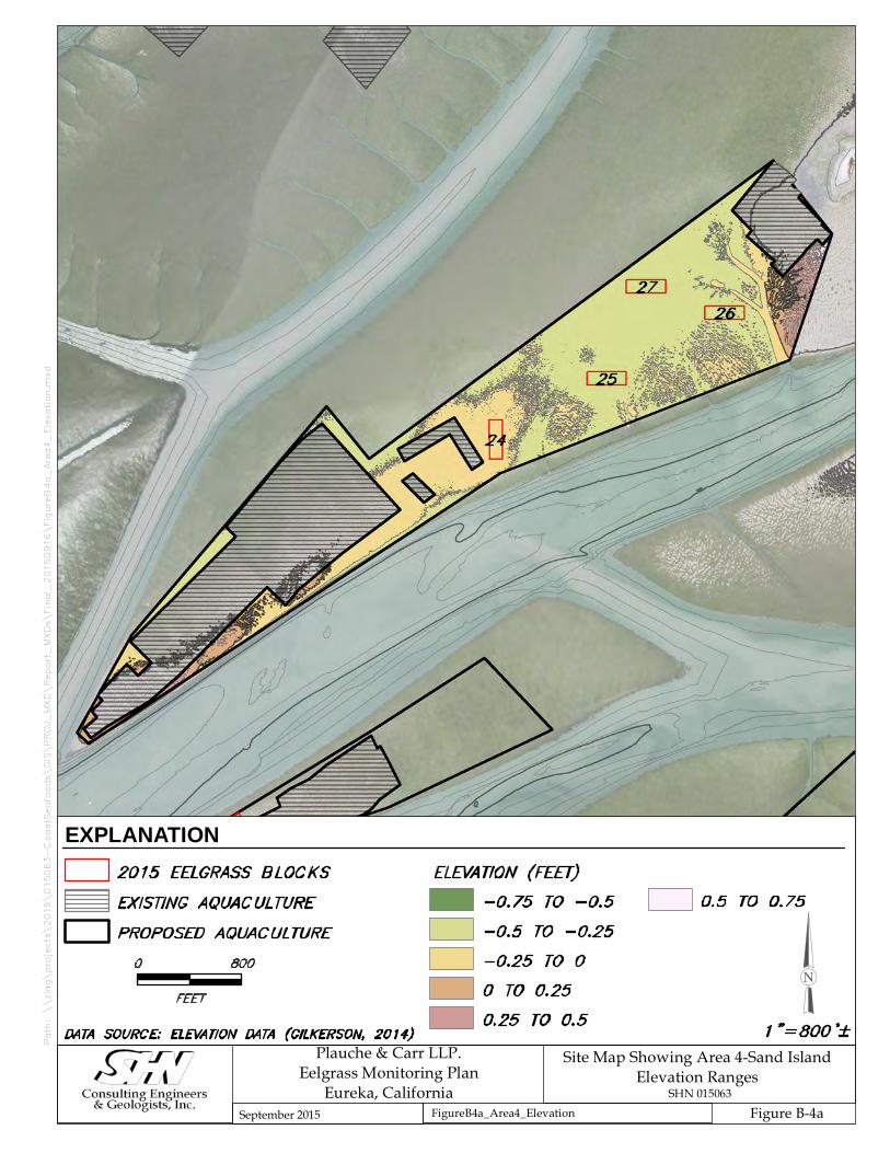
189
29
25
14
24
19
21
2627
18
1613Path: \\
zing\projects\2
015\
015063-C
oastSeafoods\G
IS\P
ROJ_MX
D\Report_
MXDs\Fina
l_20150916\Figu
reB4
a_Area4_
Elevation.mxd
Site Map Showing Area 4-Sand IslandElevation Ranges
SHN 015063Figure B-4aFigureB4a_Area4_ElevationSeptember 2015
Plauche & Carr LLP.Eelgrass Monitoring Plan
Eureka, California
1 " = 800 '±
0 800
FEET
DATA SOURCE: ELEVATION DATA (GILKERSON, 2014)
EXPLANATIONELEVATION (FEET)
-0.75 TO -0.5-0.5 TO -0.25-0.25 TO 00 TO 0.250.25 TO 0.5
0.5 TO 0.752015 EELGRASS BLOCKSEXISTING AQUACULTUREPROPOSED AQUACULTURE
189
29
25
14
24
19
21
2627
18
1613Path: \\
ZING
\Projec
ts\2015\
015063-C
oastSeafoods\G
IS\PROJ_M
XD\R
eport_MX
Ds\Fina
l_20150916\Figu
reB4
b_Area4_
SedType.m
xd
Site Map Showing Area 4-Sand IslandSediment Types
SHN 015063Figure B-4bFigureB4b_Area4_SedTypeSeptember 2015
Plauche & Carr LLP.Eelgrass Monitoring Plan
Eureka, California
1 " = 800 '±0 800
FEETDATA SOURCE: SEDIMENT TYPES (HUMBOLDT BAY HARBOR, RECREATION AND CONSERVATION DISTRICT, 2001)
EXPLANATIONSEDIMENT TYPE
CLAYEY SILTSAND-SILT-CLAYSILTY SAND
2015 EELGRASS BLOCKSEXISTING AQUACULTUREPROPOSED AQUACULTURE
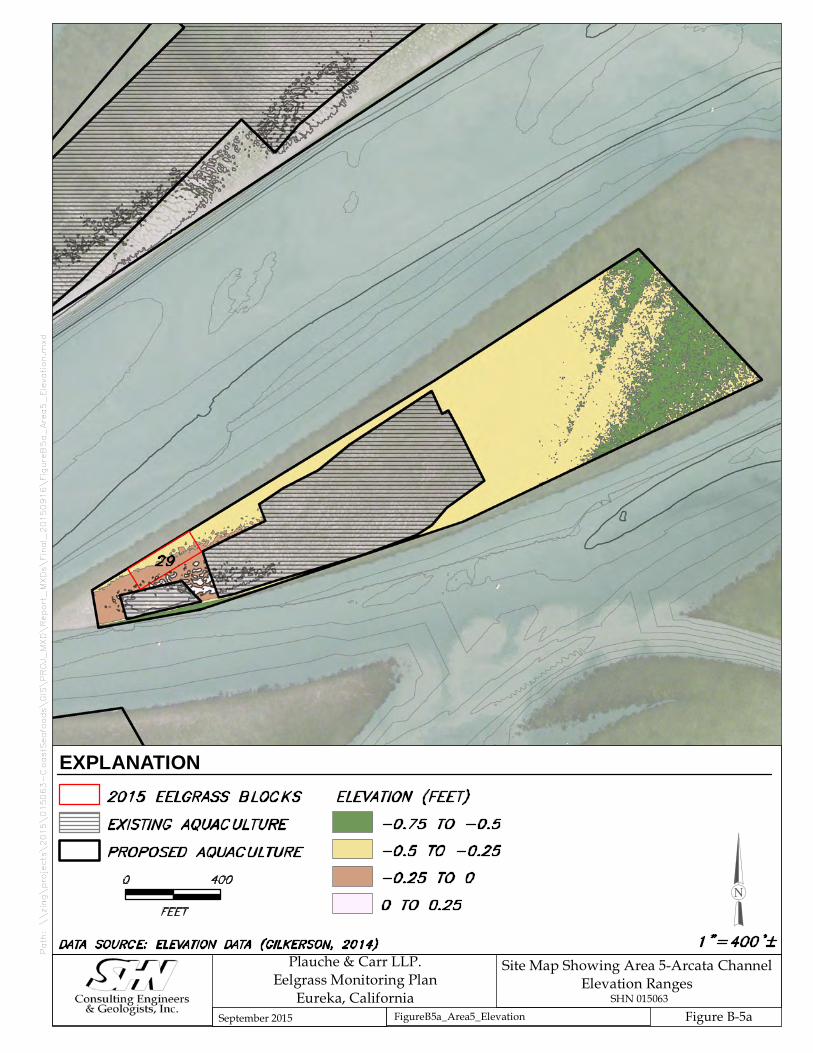
14
29
Path: \\
zing\projects\2
015\
015063-C
oastSeafoods\G
IS\P
ROJ_MX
D\Report_
MXDs\Fina
l_20150916\Figu
reB5
a_Area5_
Elevation.mxd
Site Map Showing Area 5-Arcata ChannelElevation Ranges
SHN 015063Figure B-5aFigureB5a_Area5_ElevationSeptember 2015
Plauche & Carr LLP.Eelgrass Monitoring Plan
Eureka, California
1 " = 400 '±
0 400
FEET
DATA SOURCE: ELEVATION DATA (GILKERSON, 2014)
EXPLANATIONELEVATION (FEET)
-0.75 TO -0.5-0.5 TO -0.25-0.25 TO 00 TO 0.25
2015 EELGRASS BLOCKSEXISTING AQUACULTUREPROPOSED AQUACULTURE

14
29
Path: \\
ZING
\Projec
ts\2015\
015063-C
oastSeafoods\G
IS\PROJ_M
XD\R
eport_MX
Ds\Fina
l_20150916\Figu
reB5
b_Area5_
SedType.m
xd
Site Map Showing Area 5-Arcata ChannelSediment Types
SHN 015063Figure B-5bFigureB5b_Area5_SedTypeSeptember 2015
Plauche & Carr LLP.Eelgrass Monitoring Plan
Eureka, California
1 " = 400 '±0 400
FEETDATA SOURCE: SEDIMENT TYPES (HUMBOLDT BAY HARBOR, RECREATION AND CONSERVATION DISTRICT, 2001)
EXPLANATIONSEDIMENT TYPE
SILTY SANDSAND-SILT-CLAY
2015 EELGRASS BLOCKSEXISTING AQUACULTUREPROPOSED AQUACULTURE

31
30
21
16
15
19
23
18
13
10
Path: \\
zing\projects\2
015\
015063-C
oastSeafoods\G
IS\P
ROJ_MX
D\Report_
MXDs\Fina
l_20150916\hhFigu
reB6
a_Area6_
Elevation.mxd
Site Map Showing Area 6-East Bay 2Elevation Ranges
SHN 015063Figure B-6ahhFigureB6a_Area6_ElevationSeptember 2015
Plauche & Carr LLP.Eelgrass Monitoring Plan
Eureka, California
1 " = 600 '±
0 600
FEET
DATA SOURCE: ELEVATION DATA (GILKERSON, 2014)
EXPLANATIONELEVATION (FEET)2015 EELGRASS BLOCKS
EXISTING AQUACULTUREPROPOSED AQUACULTURE
-0.75 TO -0.5-0.5 TO -0.25-0.25 TO 00 TO 0.25
0.25 TO 0.5
31
30
21
16
15
19
23
18
13
10
Path: \\
ZING
\Projec
ts\2015\
015063-C
oastSeafoods\G
IS\PROJ_M
XD\R
eport_MX
Ds\Fina
l_20150916\hhFigu
reB6
b_Area6_
SedType.m
xd
Site Map Showing Area 6-East Bay 2Sediment Types
SHN 015063Figure B-6bhhFigureB6b_Area6_SedTypeSeptember 2015
Plauche & Carr LLP.Eelgrass Monitoring Plan
Eureka, California
1 " = 600 '±0 600
FEETDATA SOURCE: SEDIMENT TYPES (HUMBOLDT BAY HARBOR, RECREATION AND CONSERVATION DISTRICT, 2001)
EXPLANATIONSEDIMENT TYPE2015 EELGRASS BLOCKS
EXISTING AQUACULTUREPROPOSED AQUACULTURE
VERY CLAYEY SILTCLAYEY SILTSAND-SILT-CLAYSILTY SAND

C Sta
tist
ical
Rev
iew
of
Co
ast
Seafo
od
s’ E
elg
rass
Mo
nit
ori
ng
Pla
n

1125 16th Street, Suite 209 Arcata, CA 95521 Ph: 707.822.4141 F: 707.822.4848
Memorandum
Project# 3225-06
4 September 2015 To: Greg O’Connell, Botanist SHN Engineers & Geologists From: Ken Lindke, Quantitative Ecologist/Fish Ecologist CC: Robert Smith, Plauché & Carr LLP; Greg Dale Coast Seafoods Company Subject: Statistical Review of Coast Seafoods’ Eelgrass Monitoring Plan (SHN 2015)
Introduction
The “Eelgrass Monitoring Plan: Coast Seafoods Company, Humboldt Bay Shellfish Culture Permit Renewal
and Expansion Project Eureka, California,” hereafter referred to as the Plan (SHN 2015), describes an
experimental study to estimate the effects of oyster aquaculture on eelgrass abundance in Humboldt Bay,
California. Several blocks are established in which eelgrass density is measured in control plots and
aquaculture plots before and after project implementation. Specific methods for estimating within-plot turion
density and evaluating changes in turion density before and after project implementation are not included in
the Plan. This memo is intended to supplement the Plan by providing guidance on these issues. Statistical
evaluation of project effects on turion density are intended satisfy the guidelines presented in “The California
Eelgrass Mitigation Policy and Implementation Guidelines,” hereafter referred to as the CEMP (National
Oceanic and Atmospheric Administration 2014). Specific quantitative methods are not provided in the
CEMP, thus the methods provided below represent our best interpretation of the author’s intentions.
Throughout this memo, the following definitions will be used, consistent with the Plan to the extent possible:
Block: any of the 30 100-foot (ft) x 300-ft experimental units that consist of each study design,
cultch-on-longline, basket-on-longline, and control.
Plot: any of the 100-ft by 100-ft experimental units consisting of one study design, either cultch-on-
longline plots, basket-on-longline plots, or control plots.
Stratum (singular)/Strata (plural): areas defined by the presence of longlines that are oriented
parallel with the longlines. Specifically these are defined as areas “under lines,” “next to lines,” and
“between lines.” No distinction is made between the many elements of a stratum within a plot; for
H. T. HARVEY & ASSOCIATES Page 2
example, all “under lines” areas within a plot are considered a single “under lines” stratum for that
plot. There are three strata in the cultch-on-longline and control plots, and four strata in the basket-
on-longline plots.
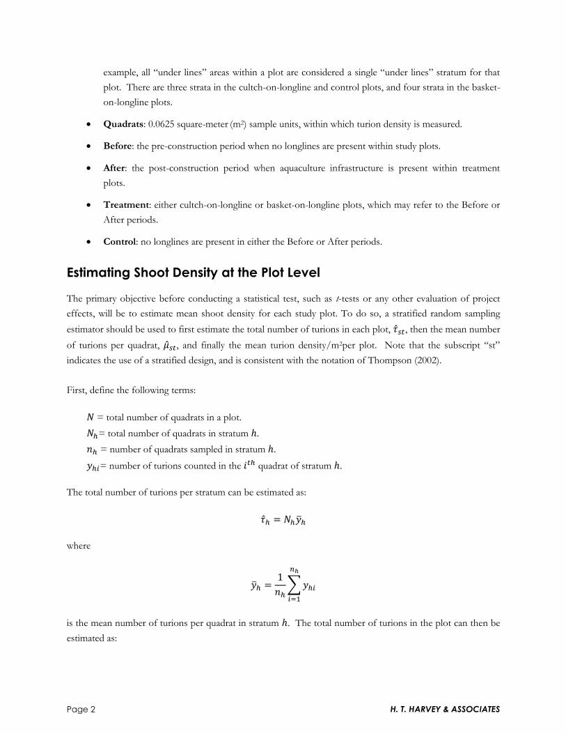
Quadrats: 0.0625 square-meter (m2) sample units, within which turion density is measured.
Before: the pre-construction period when no longlines are present within study plots.
After: the post-construction period when aquaculture infrastructure is present within treatment
plots.
Treatment: either cultch-on-longline or basket-on-longline plots, which may refer to the Before or
After periods.
Control: no longlines are present in either the Before or After periods.
Estimating Shoot Density at the Plot Level
The primary objective before conducting a statistical test, such as t-tests or any other evaluation of project
effects, will be to estimate mean shoot density for each study plot. To do so, a stratified random sampling
estimator should be used to first estimate the total number of turions in each plot, , then the mean number
of turions per quadrat, , and finally the mean turion density/m2per plot. Note that the subscript “st”
indicates the use of a stratified design, and is consistent with the notation of Thompson (2002).
First, define the following terms:
= total number of quadrats in a plot.
= total number of quadrats in stratum .
= number of quadrats sampled in stratum .
= number of turions counted in the quadrat of stratum .
The total number of turions per stratum can be estimated as:
where
is the mean number of turions per quadrat in stratum . The total number of turions in the plot can then be
estimated as:
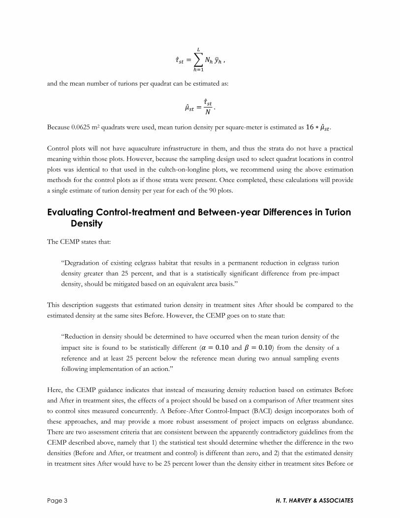
H. T. HARVEY & ASSOCIATES Page 3
and the mean number of turions per quadrat can be estimated as:
Because 0.0625 m2 quadrats were used, mean turion density per square-meter is estimated as .
Control plots will not have aquaculture infrastructure in them, and thus the strata do not have a practical
meaning within those plots. However, because the sampling design used to select quadrat locations in control
plots was identical to that used in the cultch-on-longline plots, we recommend using the above estimation
methods for the control plots as if those strata were present. Once completed, these calculations will provide
a single estimate of turion density per year for each of the 90 plots.
Evaluating Control-treatment and Between-year Differences in Turion
Density
The CEMP states that:
“Degradation of existing eelgrass habitat that results in a permanent reduction in eelgrass turion
density greater than 25 percent, and that is a statistically significant difference from pre-impact
density, should be mitigated based on an equivalent area basis.”
This description suggests that estimated turion density in treatment sites After should be compared to the
estimated density at the same sites Before. However, the CEMP goes on to state that:
“Reduction in density should be determined to have occurred when the mean turion density of the
impact site is found to be statistically different ( and ) from the density of a
reference and at least 25 percent below the reference mean during two annual sampling events
following implementation of an action.”
Here, the CEMP guidance indicates that instead of measuring density reduction based on estimates Before
and After in treatment sites, the effects of a project should be based on a comparison of After treatment sites
to control sites measured concurrently. A Before-After Control-Impact (BACI) design incorporates both of
these approaches, and may provide a more robust assessment of project impacts on eelgrass abundance.
There are two assessment criteria that are consistent between the apparently contradictory guidelines from the
CEMP described above, namely that 1) the statistical test should determine whether the difference in the two
densities (Before and After, or treatment and control) is different than zero, and 2) that the estimated density
in treatment sites After would have to be 25 percent lower than the density either in treatment sites Before or

H. T. HARVEY & ASSOCIATES Page 4
in controls After. There does not appear to be any requirement to test whether the estimated change is
statistically different than 25 percent. For example, if the estimated change was 20 percent and statistically
different than zero, but not statistically different than 25 percent, then presumably there would be no
mitigation required.
The BACI design presented in the Plan describes a paired design in which 30 blocks are randomly placed
within the project footprint, and treatment and control plots occur within those blocks. In a paired design,
two observations occurring as a pair cannot be considered independent, an important assumption when
conducting many statistical tests. In the Plan, the two plots that are paired (control and either basket-on-
longline or cultch-on-longline within a block) are immediately adjacent to each other, so if eelgrass density is
low in one it may also be low in the other, thus the two plots are not independent. Therefore, individual plot
densities cannot be used in the analysis. Instead the difference in density between the two members of each
pair is calculated, and statistical tests are conducted on these differences. Because the percent change in turion
density associated with project impacts (specifically a 25% change that is significantly different than zero) is
needed for impact assessment, the differences will be expressed as percentages relative to control plot means.
First, define the following terms:
= mean turion density in a treatment plot of the block. This is the same as above, but for a
specific treatment and block.
= mean turion density in the control plot of the block.
= standard deviations of the ’s (see below).
= the number of blocks in the study.
Then, the percent differences in mean shoot density between treatment and control plots within each block
can be calculated as:
These ’s should be calculated for each year separately, and then the data for the two years of each time
period (Before and After) can be combined to characterize each period. For a given treatment, , the mean
difference between treatment and control plots Before can be calculated simply as the average of the ’s (for
both years):
and the mean difference after construction, , can be calculated using the same equation. Comparing to
will inform the CEMP criteria for 25% decrease in abundance at treatment sites, and simultaneously meets
H. T. HARVEY & ASSOCIATES Page 5
the guidelines for comparing After impacts to Before and concurrent controls. As an example, suppose that
for cultch-on-longline is 3%, and that is -20% (negative values indicate that mean turion density in
control plots is higher than in treatment plots), then the treatment effect would be estimated as a 23%
reduction in turion density.
To test whether the difference between treatment and controls changed significantly after project
implementation, a two-sided paired t-test can be conducted for a difference between and . The test
statistic would be:
where is the unpooled standard error for the mean difference between treatment and control turion
densities:
and are the standard deviation and sample size for the ’s, and B and A refer to Before and After.
Degrees of freedom for the t-test is calculated as , assuming . If , then the
smaller of the two should be used to give a more conservative result (i.e., yielding a higher p-value).
Using a t-test to test for a difference Before and After project implementation requires that each set of ’s be
normally distributed. Examining normal probability plots, sometimes referred to as normal quantile plots, for
each of these sets should be sufficient to evaluate this assumption. If the data do not fit a normal distribution
well, the Wilcoxon signed-rank test provides a non-parametric alternative to the t-test, but with weaker
inference compared to the t-test. Methods and further details on paired t-tests and the Wilcoxon signed-rank
test can be found in most introductory statistics texts (e.g., Samuels and Witmer 2003).
References
National Oceanographic and Atmospheric Administration. 2014. California Eelgrass Mitigation Policy and
Implementation Guidelines. Final Report. October. West Coast Region.
Samuels, M. L., and J. A. Witmer. 2003. Statistics for the Life Sciences. Third edition. Prentice Hall, Upper
Saddle River, New Jersey.
[SHN] SHN Engineers and Geologists. 2015. Eelgrass Monitoring Plan: Coast Seafoods Company,
Humboldt Bay Shellfish Culture Permit Renewal and Expansion Project Eureka, California. Draft.
August. Eureka, California.

H. T. HARVEY & ASSOCIATES Page 6
Thompson, S. K. 2002. Sampling. Second edition. Wiley series in probability and statistics, New York, New
York.


