Appendix - University of California, San Diego

AppendixSignals of Responsiveness.

National Elections and European Governance

Christina J. SchneiderAssociate ProfessorJean Monnet Chair

University of California, San [email protected]

February 18, 2018

ContentsA. Appendix for Chapter 1 (Introduction) . . . . . . . . . . . . . 4

A.1. Trust in the European Union . . . . . . . . . . . . . . 4A.2. Popular Support for EU Membership . . . . . . . . . 4A.3. Perceived Government Responsiveness in European Af-

fairs . . . . . . . . . . . . . . . . . . . . . . . . . . . 6B. Appendix for Chapter 2 (The Politicization of European Co-

operation) . . . . . . . . . . . . . . . . . . . . . . . . . . . . 7B.1. Electoral Volatility in Western European States, 1950-

2010 (by Country) . . . . . . . . . . . . . . . . . . . 7B.2. Additional Measures of Saliency . . . . . . . . . . . . 8

C. Appendix for Chapter 3 (A Theory of Responsive Government) 13C.1. Voting Weights under the Nice Treaty . . . . . . . . . 13

D. Appendix for Chapter 4 (The EU-Aware Voter) . . . . . . . . 15D.1. Main Results in Tabular Form . . . . . . . . . . . . . 15D.2. Results of Unweighted Regressions . . . . . . . . . . 20D.3. Results of Weighted Regressions with Continuous Vote

Choice . . . . . . . . . . . . . . . . . . . . . . . . . 24D.4. Accounting for Political Knowledge . . . . . . . . . . 29D.5. Accounting for Attention . . . . . . . . . . . . . . . . 33

E. Appendix for Chapter 5 (The EU Budget: Financially Trivial,Politically Substantial) . . . . . . . . . . . . . . . . . . . . . 37E.1. Descriptive Statistics – Budget Models . . . . . . . . 37E.2. Model Specification – Budget Models . . . . . . . . . 38E.3. Further Robustness Checks – Budget Models . . . . . 39E.4. Interaction with Margin of Victory – Budget Models . 43E.5. Full Tables for Interaction Effects – Budget Models . . 46E.6. Descriptive Statistics – Government Approval Models 53E.7. Model Specification – Government Approval Models . 54E.8. Endogeneity – Government Approval Models . . . . . 55E.9. Net Contributors and Government Approval . . . . . . 58

2

F. Appendices for Chapter 7 (The Legislative Leviathan Mari-onette) . . . . . . . . . . . . . . . . . . . . . . . . . . . . . . 60F.1. Descriptive Statistics – Position Defending Behavior . 60F.2. Model Specification – Position Defending Behavior . . 61F.3. Robustness Checks – Position Defending Behavior . . 62F.4. Full Tables for Interaction Effects – Position Defend-

ing Behavior . . . . . . . . . . . . . . . . . . . . . . 64F.5. Descriptive Statistics – Bargaining Success . . . . . . 65F.6. Model Specification – Bargaining Success . . . . . . . 66F.7. Robustness Checks – Bargaining Success . . . . . . . 67F.8. Full Tables for Interaction Effects – Bargaining Success 69

G. Appendices for Chapter 8 (The Waiting Game) . . . . . . . . 70G.1. Model Specification – Legislative Delay . . . . . . . . 70G.2. Descriptive Statistics – Legislative Delay . . . . . . . 71G.3. Time Varying Coefficients for the Main Estimations . 72G.4. Electoral Delay Estimations for the Four Big EU Coun-

tries . . . . . . . . . . . . . . . . . . . . . . . . . . . 73G.5. Additional Robustness – Legislative Delay . . . . . . 75G.6. Do Governments Adjourn Adoptions until after Elec-

tions? . . . . . . . . . . . . . . . . . . . . . . . . . . 75H. Appendices for Chapter 9 (The Waiting Game) . . . . . . . . 82

H.1. Two Alternative Explanations – Delay Case Study . . 82

3

A. Appendix for Chapter 1 (Introduction)

A.1. Trust in the European Union

Figure A-1.: This graph displays the results of Eurobarometer surveys from2005-2015 on the question “I would like to ask you a questionabout how much trust you have in certain institutions. Foreach of the following institutions, please tell me if you tendto trust it or tend not to trust it? – European Union.” Therespondents’ answers (“tend to trust,” “tend to distrust”) aredisplayed in percentages. Data are from the interactive Euro-barometer http://ec.europa.eu/COMMFrontOffice/PublicOpinion/index.cfm/Chart/index, last ac-cessed: September 2016)

A.2. Popular Support for EU Membership

4

http://ec.europa.eu/COMMFrontOffice/PublicOpinion/index.cfm/Chart/index


Figure A-2.: This graph displays the results of Eurobarometer surveysfrom 1973-2015 on the question “Generally speaking, doyou think that (your country’s) membership of the Euro-pean Union is a good thing, a bad thing, or neither goodnor bad?” The respondents’ answers are displayed inpercentages. Data are from the interactive Eurobarom-eter http://ec.europa.eu/COMMFrontOffice/PublicOpinion/index.cfm/Chart/index, last ac-cessed: September 2016)

5



A.3. Perceived Government Responsiveness inEuropean Affairs

This graph displays the results of Eurobarometer surveys from 2005-2015 on the question “Please tell me for each statement, whether youtend to agree or tend to disagree?: The interests of (OUR COUN-TRY) are well taken into account in the EU.” The respondents’ answers(“agree,” “disagree”) are displayed in percentages. Data are from the inter-active Eurobarometer http://ec.europa.eu/COMMFrontOffice/PublicOpinion/index.cfm/Chart/index, last accessed: Septem-ber 2016)

6



B. Appendix for Chapter 2 (The Politicizationof European Cooperation)

B.1. Electoral Volatility in Western European States,1950-2010 (by Country)

01

02

03

04

00

10

20

30

40

01

02

03

04

00

10

20

30

40

1940 1960 1980 2000 2020

1940 1960 1980 2000 2020 1940 1960 1980 2000 2020 1940 1960 1980 2000 2020

Austria Belgium Denmark Finland

France Germany Greece Ireland

Italy Luxembourg Portugal Spain

Sweden The Netherlands United Kingdom

Ele

cto

ral V

ola

tilit

y

Election YearGraphs by Country

The graph displays the Pedersen index of electoral volatility in 15 Western Eu-ropean countries from 1950-2010. Source: Dassonneville and Hooghe (2017).

7

B.2. Additional Measures of SaliencyOne question that has been ask repeatedly (although unfortunately not fre-quently throughout time) is a question about the importance of the EU to citi-zen of EU countries:

“Whether or not you have the time to take personal interest in theproblems of the European Community, do you feel that these prob-lems are very important, important, not very important or unim-portant for the future of *country* and the people of *country*?”

Table B-1 provides information on the average level of importance that Eu-ropeans have attached to the European Communities in 1975 and 1991 (theearliest and latest year for which this question was included in the Eurobarom-eter surveys).1 In 1975, about 75% of respondents thought that the EuropeanCommunity was very important or important, and about 15% believed the Eu-ropean Communities to be not very important or unimportant. The numbers in1991 are 83% and 11%, respectively. Whereas there may not be a significanttrend across time, the high level of importance that individuals attribute to theEU over time is very indicative of the assumption that voters should care aboutwhether their governments are competent in EU negotiations.

Of course, the importance of the EU varies across EU member countries.Table B-2 presents the results for a selection of EU member states. Across sur-veys, about 80% of EU citizens think that the EU is important, and 13% thinkthat it is not important. But whereas almost 35% of UK citizens believe thatthe EU is very important, only 20% of Belgium citizens and 22% of Germancitizens have the same opinion. Likewise, most individuals in Portugal believethat the EU is very important or important, and only 1.85% believe that theEU is unimportant. In France, on the other hand, almost 5% of respondentsbelieve that the EU is unimportant.

Another question that relates to the general salience of European politics onthe domestic level is the extent to which individuals are interested in mattersrelated to the EU:

“To what extent would you say you are interested in European Pol-itics, that is to say matters related to the European Community?”

1Unfortunately, none of the questions about citizen’s interest in the EU or the importancethat they attribute to the EU have been asked after the early 1990s.

8

1975 1991(% of Respondents)

Very Important 32.69 35.02Important 42.11 48.32Not Very Important 10.75 8.37Unimportant 4.65 2.26

Table B-1.: EU Importance within the European Union. The graph displays theresults of Eurobarometer surveys from 2005-2013 on the question“Whether or not you have the time to take personal interest in theproblems of the European Community, do you feel that these prob-lems are very important, important, not very important or unimpor-tant for the future of *country* and the people of *country*?” Theresponses (“Very Important,” “Important,” “Not Very Important,”“Unimportant”) are displayed in percentages. Source: Schmittet al. (2005)

Table B-3 shows that in 1988 (the earliest year for which this question wasincluded in the Eurobarometer survey) about 39% of EU citizens cared a greatdeal or at least to some extent about European politics. In 1994 (the latestyear for which this question was included in the Eurobarometer survey), thenumber rose slightly to 42%. The number of EU citizens who were not muchor not at all interested in the EU dropped slightly from about 59% to 52%.Nevertheless, at least in 1994 a majority of citizen in the European Unionstill did not care a great deal about the EU despite the existence of a singleEuropean market and the beginning of the European Monetary Union.

Table B-4 indicates that this trend varies across EU members. Overall, thereis no majority of EU citizens who believe the EU is not important (the averageacross years is about 45% which is almost on par with the share of individualswho are interested in the EU). French respondents appear to be amongst themost interested citizens (47%), whereas Portuguese respondents are amongstthe least interested (28%). 31% of Portuguese are not at all interested in Euro-pean matters. This compares to much lower numbers in Germany (12.60%).

Finally, it is worth looking at the salience of EU issues in the domesticmedia. The Eurobarometer includes questions about the extent to which indi-

9

All France Belgium Germany UK Portugal(% of Respondents)

Very Important 30.51 30.53 20.39 22.68 34.70 22.27Important 49.90 52.03 51.85 52.37 45.70 53.57Not Very Important 9.81 9.53 13.35 15.57 11.24 6.04Unimportant 3.38 4.98 3.90 2.93 3.84 1.85

Table B-2.: EU Importance Across EU Countries The graph displays the re-sults of Eurobarometer surveys from 2005-2013 on the question“Whether or not you have the time to take personal interest in theproblems of the European Community, do you feel that these prob-lems are very important, important, not very important or unimpor-tant for the future of *country* and the people of *country*?” Theresponses (“Very Important,” “Important,” “Not Very Important,”“Unimportant”) are displayed in percentages. Source: Schmittet al. (2005)

viduals read about the EU in the papers, on radio, or on television:

“Have you recently seen or heard in the papers, on the radio, or ontelevision, anything about the European Commission in Brussels,that is the Commission of the European Community?”

Table B-5 shows that whereas a majority of European citizens had not reador heard about the EU in the media in 1987, a majority of respondents recentlyread or heard about the EU in 1992. The share of respondents recently exposedto news about the EU rose from about 45% to 50%, with a similar decline inthose who had not heard about the EU in the media.

10


A Great Deal 8.89 9.17To Some Extent 30.30 31.36Not Much 35.33 33.02Not At All 23.81 19.69

Table B-3.: Public EU Interest within the European Union. The graph dis-plays the results of Eurobarometer surveys from 2005-2013 onthe question “To what extent would you say you are interested inEuropean Politics, that is to say matters related to the EuropeanCommunity?” The responses (“A Great Deal,” “To Some Extent,”“Not Much,” “Not At All”) are displayed in percentages. Source:Schmitt et al. (2005)

All France Belgium Germany UK Portugal(% of Respondents)

A Great Deal 9.67 11.31 7.07 9.66 9.79 5.73To Some Extent 32.81 36.15 30.32 34.21 35.92 22.07Not Much 25.80 33.56 35.90 41.97 32.17 37.80Not At All 19.31 17.05 24.81 12.60 21.21 31.03

Table B-4.: Public EU Interest Across EU Countries. The graph displays theresults of Eurobarometer surveys from 2005-2013 on the question“To what extent would you say you are interested in European Pol-itics, that is to say matters related to the European Community?”The responses (“A Great Deal,” “To Some Extent,” “Not Much,”“Not At All”) are displayed in percentages. Source: Schmitt et al.(2005)

11


Yes 44.88 50.04No 49.08 43.48

Table B-5.: Media Salience. The graph displays the results of Eurobarome-ter surveys from 2005-2013 on the question “Have you recentlyseen or heard in the papers, on the radio, or on television, anythingabout the European Commission in Brussels, that is the Commis-sion of the European Community?” The responses (“Yes,” “No”)are displayed in percentages. Source: Schmitt et al. (2005)

12

C. Appendix for Chapter 3 (A Theory ofResponsive Government)

C.1. Voting Weights under the Nice TreatyEach government’s votes in the Council are weighted roughly by populationsize. With each enlargement, the number of votes for each member has changed,but the ranking of member states by the number of votes they has stayedroughly the same over time, until voting weights were abolished with LisbonTreaty in 2009 (the reform took effect in November 2014). Table C-6 presentsthe distribution of votes across EU members in the EU-28. Germany, France,Italy, and the United Kingdom receive most votes, but some new members(notably Poland) have received a large number of votes upon accession to theEU in the last decade.

Country Votes Votes (%)Germany, France, Italy, UK 29 8.2Poland, Spain 27 7.7Romania 14 4.0Netherlands 13 3.7Belgium, Czech Republic, Greece, Hungary, Portugal 12 3.4Austria, Bulgaria, Sweden 10 2.8Croatia, Denmark, Finland, Ireland, Lithuania, Slovakia 7 2.0Cyprus, Estonia, Latvia, Luxembourg, Slovenia 4 1.1Malta 3 0.9

Total 352 100

Table C-6.: Distribution of Votes in the Council, EU-28. The ta-ble displays the official number of votes and vote sharesof EU member countries as decided with the LisbonTreaty in 2009. Source: Council of the EU at http://www.consilium.europa.eu/en/council-eu/voting-system/qualified-majority/, last accessed:September 2016.

13

http://www.consilium.europa.eu/en/council-eu/voting-system/qualified-majority/



It is interesting to note that there is a bias towards the smaller countries in theEU. EU members are extremely asymmetrical in terms of their population size(you just need to compare Germany with 80 million citizen to Luxembourgwith 500,000 citizen), and a weighting of votes according to population sizewould prevent small EU member states from having any meaningful influencein the Council. The EU therefore gives disproportionally more votes to smallEU countries. Table C-7 illustrates this. Whereas Germany has only 0.36votes for each one million German citizen, Luxembourg has 8 votes per onemillion Luxembourg citizen. It has therefore been argued that small states havedisproportional influence on EU decision-making (Rodden, 2002; Aksoy andRodden, 2009; Aksoy, 2010).

The three criteria for decisions to be adopted under the Nice rules were74% of member states’ weighted votes, cast by a majority of member states,and optionally, a check that the majority represented at least 62% of the EU’sentire population. Many criticized that the thresholds were too high, leadingto substantial gridlock in Council decision-making. As discussed in Chapter2, the voting reform under the Lisbon Treaty in 2009 attempted to rectify theseproblems.

Country Votes Population Per Capita Votes(in million) (in million)

Germany 29 80 0.36Poland 27 38.5 0.70Netherlands 13 16.8 0.77Portugal 12 10.4 1.15Croatia 7 4.2 1.67Luxembourg 4 0.5 8Malta 3 0.4 7.5

Table C-7.: Council Votes and Representation in the EU-28. Distribution ofVotes in the Council, EU-28. The table displays the official num-ber of votes, population size, and per capita of EU member coun-tries as decided with the Lisbon Treaty in 2009. Source: Councilof the EU, Eurostat, and own calculations.

14

D. Appendix for Chapter 4 (The EU-AwareVoter)

D.1. Main Results in Tabular Form

15

(Bailout) (Refugees)Support Opposition Support Opposition

Position Affinity 0.010 0.022** 0.022* 0.024**(0.009) (0.009) (0.011) (0.009)

Vote Affinity 0.024** 0.030** 0.020** 0.048**(0.010) (0.010) (0.010) (0.010)

Outcome Affinity 0.005 0.024** 0.011 0.049**(0.009) (0.008) (0.011) (0.010)

Partisanship 0.065** 0.045** 0.030* 0.060**(0.019) (0.015) (0.018) (0.023)

Gender 0.021** 0.002 -0.005 0.009(0.009) (0.009) (0.009) (0.009)

Experience (2) 0.001 -0.044** -0.000 -0.000(0.017) (0.017) (0.018) (0.013)

Experience (4) 0.010 -0.027 0.005 -0.005(0.017) (0.016) (0.017) (0.016)

Experience (6) -0.001 -0.037** 0.004 0.013(0.014) (0.015) (0.019) (0.016)

Experience (8) -0.010 -0.037** -0.000 -0.003(0.015) (0.017) (0.017) (0.013)

Experience (10) 0.030** -0.021 0.013 0.001(0.015) (0.015) (0.018) (0.015)

Constant 0.460** 0.486** 0.469** 0.431**(0.013) (0.014) (0.016) (0.013)

Observations 2080 2364 1960 2484Standard errors in parentheses* p<0.10, ** p<0.05

Table D-8.: Weighted Sample Model Results - Position Affinity

16

(Bailout) (Refugees)Responsive Nonresponsive Responsive Nonresponsive

Defense 0.031** -0.024* 0.036** -0.037**(0.011) (0.013) (0.013) (0.011)

Position -0.010 -0.004 -0.004 0.000(0.007) (0.007) (0.007) (0.008)

Vote -0.008 0.002 -0.006 -0.022*(0.011) (0.013) (0.012) (0.012)

Outcome -0.007 -0.015 -0.009 -0.038**(0.011) (0.011) (0.013) (0.013)

Partisanship 0.071** 0.038* 0.043 0.041(0.023) (0.022) (0.026) (0.027)

Gender 0.009 0.014 0.008 -0.002(0.012) (0.011) (0.011) (0.012)

Experience (2) -0.025 -0.020 -0.005 0.004(0.019) (0.019) (0.018) (0.020)

Experience (4) -0.029 0.006 -0.006 0.009(0.020) (0.018) (0.021) (0.022)

Experience (6) -0.042** 0.006 -0.011 0.033(0.018) (0.018) (0.019) (0.022)

Experience (8) -0.030 -0.018 0.006 -0.013(0.018) (0.021) (0.018) (0.021)

Experience (10) -0.015 0.017 0.012 -0.002(0.020) (0.017) (0.020) (0.022)

Constant 0.519** 0.505** 0.496** 0.531**(0.017) (0.016) (0.017) (0.020)


Table D-9.: Weighted Sample Model Results - Position-Defending Behavior

17

(Bailout) (Refugees)Responsive Nonresponsive Responsive Nonresponsive

Success 0.026** -0.005 0.030** -0.030**(0.011) (0.012) (0.013) (0.012)

Position Affinity -0.012 -0.002 0.005 -0.014(0.012) (0.011) (0.012) (0.013)

Vote Affinity -0.006 -0.001 -0.014** -0.011(0.007) (0.008) (0.007) (0.007)

Outcome Affinity -0.012 -0.009 -0.027** -0.009(0.011) (0.012) (0.013) (0.012)

Partisanship 0.059** 0.044** 0.035 0.051**(0.022) (0.021) (0.025) (0.025)

Gender 0.029** -0.007 -0.002 0.007(0.011) (0.012) (0.011) (0.011)

Experience (2) -0.019 -0.021 0.012 -0.016(0.021) (0.021) (0.019) (0.018)

Experience (4) -0.007 -0.008 0.019 -0.023(0.019) (0.021) (0.021) (0.021)

Experience (6) -0.019 -0.015 0.011 0.009(0.017) (0.019) (0.020) (0.019)

Experience (8) -0.029 -0.010 0.011 -0.020(0.018) (0.021) (0.019) (0.018)

Experience (10) -0.016 0.023 0.011 0.000(0.018) (0.018) (0.019) (0.019)

Constant 0.511** 0.501** 0.506** 0.517**(0.017) (0.016) (0.018) (0.017)


Table D-10.: Weighted Sample Model Results - Bargaining Success

18

(Bailout) (Refugees)Support Opposition Support Opposition

Competence 0.025** 0.001 0.023** 0.024**(0.010) (0.010) (0.010) (0.009)

Position Affinity 0.019* 0.059** 0.027** 0.048**(0.010) (0.010) (0.009) (0.011)

Outcome Affinity 0.024* 0.030** -0.000 0.050**(0.013) (0.008) (0.011) (0.010)

Partisanship 0.043** 0.056** 0.038** -0.001(0.019) (0.020) (0.017) (0.021)

Gender 0.019* 0.022** -0.028** 0.012(0.011) (0.009) (0.009) (0.010)

Experience (2) 0.012 -0.005 0.016 -0.029*(0.017) (0.017) (0.021) (0.017)

Experience (4) 0.016 0.011 0.002 0.006(0.020) (0.015) (0.019) (0.018)

Experience (6) 0.021 0.017 0.012 -0.012(0.017) (0.018) (0.019) (0.017)

Experience (8) 0.030 -0.000 0.016 -0.013(0.020) (0.013) (0.020) (0.018)

Experience (10) 0.021 -0.003 0.022 -0.002(0.020) (0.018) (0.018) (0.016)

Constant 0.438** 0.439** 0.475** 0.440**(0.018) (0.014) (0.017) (0.015)


Table D-11.: Weighted Sample Model Results - Negotiation Competence

19

D.2. Results of Unweighted Regressions

close

close

close

same

same

2

4

6

8

10

Position Affinity

Vote Affinity

Outcome Affinity

Partisanship

Gender

Experience

−.1 −.05 0 .05 .1 −.05 0 .05 .1

Bailout Refugees

Voters in favor of the policy Voters opposed to the policy

Change in the probability of voting for the politician

Figure D-3.: Position-Taking and Voter Support. Marginal component-specific ef-fects from a linear probability model. Bars denote 90% confidence intervals.Reference values for each variable omitted.

20

yes

in favor

in favor

in favor

same

same

2468

10

Defense

Position

Vote

Outcome

Partisanship

Gender

Experience

−.05 0 .05 .1 −.05 0 .05 .1

Bailout Refugees

Voters with policy position similar politician’s

Voters with policy position different from politician’s


Figure D-4.: Position-Defending and Voter Support. Marginal component-specificeffects from a linear probability model. Bars denote 90% confidence intervals.Reference values for each variable omitted.

21

yes

in favor

in favor

in favor

same

same

2468

10

Success

Position

Vote

Outcome

Partisanship

Gender

Experience

−.05 0 .05 .1 −.05 0 .05 .1

Bailout Refugees

Voters with policy position similar to politician’s vote

Voters with policy position different from politician’s vote

Change in the Probability of Voting for the Politician

Figure D-5.: Credit-Claiming and Voter Support. Marginal component-specific ef-fects from a linear probability model. Bars denote 90% confidence intervals.Reference values for each variable omitted.

22

high

close

close

same

same

2

4

6

8

10

Competence

Position Affinity

Outcome Affinity

Partisanship

Gender

Experience

−.05 0 .05 .1 −.05 0 .05 .1

Bailout Refugees

Voters in favor of the policy

Voters opposed to the policy


Figure D-6.: Negotiation Competence and Voter Support. Marginal component-specific effects from a linear probability model. Bars denote 90% confidenceintervals. Reference values for each variable omitted.

23

D.3. Results of Weighted Regressions withContinuous Vote Choice

This section provides the results for re-estimating all main regressions, usingas the dependent variable the continuous vote choice of respondents. In par-ticular, after respondents decided which of the politicians they would prefer inthe comparisons, I further ask them the following question:

If there was an election this Sunday, how likely would you votefor each of these politicians?

Respondents rated each politician individually on a scale from 1 (very un-likely) to 10 (very likely).2 The following tables present results using thisdependent variable. The estimations are based on the re-weighted data (seeprevious section for a discussion).

2The order of categories was reversed for half of the respondents.

24

close

close

close

same

same

2

4

6

8

10

Position Affinity

Vote Affinity

Outcome Affinity

Partisanship

Gender

Experience

−1 0 1 2 −1 −.5 0 .5 1

Bailout Refugees




25

yes

in favor

in favor

in favor

same

same

2468

10

Defense

Position

Vote

Outcome

Partisanship

Gender

Experience

−1 0 1 2 −1 −.5 0 .5 1

Bailout Refugees

Voters with policy position similar to politician’s



Figure D-8.: Position-Defending and Voter Support. Marginal component-specificeffects from a linear probability model. Bars denote 90% confidence intervals.Reference values for each variable omitted.

26

yes

in favor

in favor

in favor

same

same

2468

10

Success

Position

Vote

Outcome

Partisanship

Gender

Experience

−.5 0 .5 1 1.5 −1 −.5 0 .5 1

Bailout Refugees





27

high

close

close

same

same

2

4

6

8

10

Competence

Position Affinity

Outcome Affinity

Partisanship

Gender

Experience

−1 0 1 2 −.5 0 .5 1 1.5

Bailout Refugees




28

D.4. Accounting for Political KnowledgeThis section provides the results for re-estimating all main regressions on asub-sample that only includes respondents that answered at least two out ofthree political knowledge questions correctly. The three questions were:

1. Who is currently the minister of defense in Germany?

2. Which party received the largest number of seats in the German parlia-ment in the general elections of 2013?

3. For how many years are members of the German parliament elected?

close

close

close

same

same

2

4

6

8

10

Position Affinity

Vote Affinity

Outcome Affinity

Partisanship

Gender

Experience

−.1 −.05 0 .05 .1 −.05 0 .05 .1

Bailout Refugees




29

yes

in favor

in favor

in favor

same

same

2468

10

Defense

Position

Vote

Outcome

Partisanship

Gender

Experience

−.1 −.05 0 .05 .1 −.05 0 .05 .1

Bailout Refugees




Figure D-12.: Position-Defending and Voter Support. Marginal component-specific effects from a linear probability model. Bars denote 90% confidenceintervals. Reference values for each variable omitted.

30

yes

in favor

in favor

in favor

same

same

2468

10

Success

Position

Vote

Outcome

Partisanship

Gender

Experience

−.05 0 .05 .1 −.05 0 .05 .1

Bailout Refugees





31

high

close

close

same

same

2

4

6

8

10

Competence

Position Affinity

Outcome Affinity

Partisanship

Gender

Experience

−1 0 1 2 −1 0 1 2

Bailout Refugees




32

D.5. Accounting for AttentionThis section provides the results for re-estimating all main regressions on asub-sample that only includes respondents that passed a relatively stringentattention test. Respondents had to answer the following question:

“We are interested in a number of different topics, including col-ors. To show that you read this text, please pick the colors redand green from the alternatives below, regardless of your actualfavorite color. Yes, please ignore the following question and pickthose two colors. What is your favorite color”

The graphs present the results from estimations that only include respon-dents who answered the question correctly.

close

close

close

same

same

2

4

6

8

10

Position Affinity

Vote Affinity

Outcome Affinity

Partisanship

Gender

Experience

−.1 −.05 0 .05 .1 −.05 0 .05 .1 .15

Bailout Refugees




33

yes

in favor

in favor

in favor

same

same

2468

10

Defense

Position

Vote

Outcome

Partisanship

Gender

Experience

−.1 −.05 0 .05 .1 −.05 0 .05 .1

Bailout Refugees




Figure D-16.: Position-Defending and Voter Support. Marginal component-specific effects from a linear probability model. Bars denote 90% confidenceintervals. Reference values for each variable omitted.

34

yes

in favor

in favor

in favor

same

same

2468

10

Success

Position

Vote

Outcome

Partisanship

Gender

Experience

−.1 −.05 0 .05 .1 −.05 0 .05 .1 .15

Bailout Refugees





35

high

close

close

same

same

2

4

6

8

10

Competence

Position Affinity

Outcome Affinity

Partisanship

Gender

Experience

−1 0 1 2 −1 0 1 2

Bailout Refugees




36

E. Appendix for Chapter 5 (The EU Budget:Financially Trivial, Politically Substantial)

E.1. Descriptive Statistics – Budget Models

Mean SD Min MaxESIF Receipts (%) 1.390681 1.676589 .0011971 9.189159CAP Receipts (%) 3.271311 3.622601 .0019641 17.48617Budget Receipts (%) 5.276276 4.945518 .018287 20.83979Election Period .5204461 .5000467 0 1Agricultural Sector (ln, t-1) 5.372428 1.567243 1.280934 8.05484GDP (ln, t-1) 12.19899 1.531555 8.475266 14.80992Per Capita GDP (ln, t-1) -3.951779 .5554865 -5.650322 -2.494962Unemployment (%) 8.219145 3.746008 .7 22Voting Power (%) 6.224363 4.437807 .9524 17.8571Public EU Support .4281165 .2206227 -.255 .86New Member State .1672862 .3735786 0 1EU Membership Size 18.60781 6.908318 9 27N 538

37

E.2. Model Specification – Budget ModelsThe time-series cross-sectional nature of the data raises concerns of panel het-eroscedasticity and serial correlation. I estimate an unbalanced panel modelwith fixed effects. The fixed effects estimator controls for unobserved countryheterogeneity that is constant over time. This procedure is warranted becausethe time independent country effects turn out significant in the regression andthe results of the Hausman test suggests that alternatives would render the coef-ficients inconsistent and biased. Note, I show below that the results are robustto including year fixed effects or using random effects. One potential issuewith estimating panel models using budget shares as a dependent variable isthat all budget shares in any given year sum up to 100%. The compositionalnature of the variable puts constraints on the aid shares that countries can re-ceive. In the robustness tests below, I show that the results are robust whentaking the compositional structure of the data into account.

All models have panel-corrected standard errors (PCSEs) to correct for panelheteroscedasticity as well as for contemporaneously correlated errors acrosspanels. Whereas a PCSE model can deal with unbalanced panel data, I alsoinclude a variable measuring the number of members in each year in order toaccount for increasing number of panels over time. Using EU size dummiesinstead does not substantially alter the findings.

Additionally, the Durbin Watson statistic of an untransformed model pointsto a serial correlation of the error terms. The main specifications use a PraisWinsten transformation of the error term (AR1 process). In the main mod-els I use panel-specific transformations of the error term, but I show in therobustness checks below that the results are robust to using a general AR1autocorrelation structure.

38

E.3. Further Robustness Checks – Budget ModelsIn earlier work, on which this analysis is build, I show that the models arerobust to a number of different model specifications (Schneider, 2013):

1. Endogenous election timing (robust)

2. Importance of snap elections (robust)

3. Alternative operationalizations of the main independent variable:

• Continuous election indicator (robust)

• Presidential elections (no effect as expected)

• Year to election (no effect)

• Postelection dummy (no effect)

4. Alternative Dependent Variable:

• Total Net Receipts (robust)

5. Additional Control Variables:

• Financial Frameworks (robust)

• Partisan Extremity (robust)

6. Model Specification:

• Lagged dependent variable (robust)

• System general methods of moments estimator (robust)

In addition to the robustness checks that I conducted in Schneider (2013),I now provide some additional robustness checks. Model 1 in Table E-12presents the main estimation without country fixed effects. Model 2 includescountry and year fixed effects, and Model 3 presents the ESIF Shares modelfor the period from 1977-2004 to analyze whether countries with higher pcGDP received fewer structural transfers before the enlargement to Central andEastern European countries (see discussion of the results in Table 5.1). Themain effect is robust to these changes in the model specification, and I also findas expected that poorer countries indeed received greater ESIF shares beforeenlargement. The puzzling result in the main tables therefore owes most likely

39

to the distribution of income across old and new member states after Easternenlargement. In addition, whereas I use a panel-specific transformation of theerror term in the main model, Model 4 demonstrates that the results are robustto using an AR1 autocorrelation structure that is not specific to the particularpanel. One potential issue with using budget shares is that all budget sharesin any given year sum up to 100%. The compositional nature of the variableputs constraints on the aid shares that countries can receive. To address thisproblem, I calculated an unconstraint model that use the log of total aid receiptsas a dependent variable (Model 5). Following Aitchison (2003), I also log-transformed the data by creating a log budget ratio between a country’s budgetshares, and the other EU members’ budget shares (Model 6). The advantageof the log-transformation proportional outcome is that it is unconstrained. Themain results are robust in both cases.

Table E-13 analyzes whether the budget cycles are dependent on one of thebig four in the EU (UK, Germany, Italy, France). It indicates expectedly thatbudget cycles are indeed much weaker if we exclude observations for the UKand France, but that budget cycles would be stronger without Germany andItaly in the sample. In general, the electoral cycle persists (sometimes weakly)even if we exclude countries from the sample.

40

(1)

(2)

(3)

(4)

(5)

(6)

Ran

dom

Eff

ects

Yea

rFE

ESI

F(b

efor

e20

04)

AR

Proc

ess

Tota

lRec

eipt

s(l

n)L

ogTr

ansf

orm

edD

VE

lect

ion

Peri

od0.

118*

*0.

098*

*0.

053

0.10

5*0.

030*

*0.

034*

*(0

.038

)(0

.044

)(0

.044

)(0

.056

)(0

.012

)(0

.012

)A

gric

ultu

ralS

ecto

r(ln

,t-1

)1.

316*

*-1

.250

**-1

.123

**1.

054*

*-0

.450

**-0

.016

(0.1

39)

(0.3

64)

(0.3

07)

(0.4

32)

(0.1

16)

(0.1

08)

GD

P(l

n,t-

1)-0

.566

**3.

342*

*1.

536*

-5.9

73**

0.52

8-0

.854

**(0

.188

)(1

.075

)(0

.856

)(1

.162

)(0

.333

)(0

.419

)Pe

rCap

itaG

DP

(ln,

t-1)

2.55

4**

-0.4

08-2

.683

**7.

002*

*0.

168

1.38

5**

(0.3

34)

(1.0

70)

(0.9

63)

(1.1

93)

(0.3

13)

(0.4

19)

Une

mpl

oym

ent(

%)

0.08

0**

0.04

0*-0

.034

**0.

015

0.01

6**

0.01

4**

(0.0

21)

(0.0

21)

(0.0

16)

(0.0

25)

(0.0

07)

(0.0

06)

Votin

gPo

wer

(%)

0.75

3**

0.49

4**

-0.0

59**

0.66

0**

0.03

2*0.

097*

*(0

.052

)(0

.055

)(0

.027

)(0

.076

)(0

.017

)(0

.017

)Pu

blic

EU

Supp

ort

0.24

6-0

.180

-1.3

30**

-1.1

39**

-0.1

37-0

.319

**(0

.410

)(0

.363

)(0

.264

)(0

.422

)(0

.104

)(0

.104

)N

ewM

embe

rSta

te-0

.881

**-1

.125

**-0

.908

**-0

.961

**-0

.159

**-0

.180

**(0

.157

)(0

.138

)(0

.235

)(0

.145

)(0

.062

)(0

.061

)E

UM

embe

rshi

pSi

ze0.

050*

*-0

.397

**0.

016*

0.05

6**

-0.0

11-0

.003

(0.0

25)

(0.0

36)

(0.0

09)

(0.0

25)

(0.0

08)

(0.0

07)

Con

stan

t8.

883*

*-2

8.73

4*-2

2.64

594

.762

**3.

979

12.0

02*

(2.3

98)

(16.

934)

(14.

085)

(18.

506)

(5.4

64)

(6.8

51)

Obs

erva

tions

553

553

333

553

553

553

Wal

dTe

stch

i223

08.3

0953

4587

93.3

8324

3127

6.23

243

810.

951

1060

315.

865

2469

267.

743

Stan

dard

erro

rsin

pare

nthe

ses

*p<

0.10

,**

p<0.

05

Tabl

eE

-12.

:Mod

elSp

ecifi

catio

n

41

(1) (2) (3) (4)No UK No Germany No France No Italy

Election Period 0.078* 0.145** 0.072* 0.125**(0.048) (0.047) (0.044) (0.045)

Agricultural Sector (ln, t-1) 1.199** 1.445** 1.087** 0.632*(0.393) (0.372) (0.364) (0.326)

GDP (ln, t-1) -3.407** -11.093** -3.277** -5.814**(1.258) (1.356) (1.067) (1.186)

Per Capita GDP (ln, t-1) 4.334** 12.735** 4.208** 6.345**(1.261) (1.543) (1.074) (1.151)

Unemployment (%) 0.014 0.032 0.017 0.017(0.025) (0.023) (0.024) (0.022)

Voting Power (%) 0.627** 0.742** 0.701** 0.616**(0.075) (0.069) (0.057) (0.067)

Public EU Support -0.577 -1.447** -1.250** -1.397**(0.415) (0.386) (0.399) (0.393)

New Member State -1.044** -1.020** -1.010** -1.046**(0.164) (0.143) (0.148) (0.141)

EU Membership Size 0.038 0.076** 0.062** 0.055**(0.028) (0.024) (0.025) (0.025)

Constant 53.027** 177.672** 50.910** 93.030**(20.029) (21.510) (17.098) (18.778)

Observations 518 518 518 518Wald Testchi2 329724.467 189105.786 1066481.257 164408.714Standard errors in parentheses* p<0.106, ** p<0.05

Table E-13.: Testing for Country Dependency

42

E.4. Interaction with Margin of Victory – BudgetModels

Whereas my measure of government approval is preferable to retrospectivemeasures of electoral competition because it is prospective, it cannot take intoaccount competition with other parties, which may increase electoral uncer-tainty dramatically. To account for competition between parties (i.e. the close-ness of an election), I created two measures. The first measure uses the ap-proval data, but generates the difference between the incumbent party with thestrongest approval and the party with the second strongest approval (could bepart of the incumbent coalition or the opposition).3 Second, I use the retrospec-tive measure of the actual difference between the party that received the great-est vote share and the party that received the second largest vote share. Datafor the retrospective margin of victory measure are from Doring and Manow(2015).

Figure E-19 presents the results. Subfigure E-19(a) is particularly inter-esting because it reveals some of the limitations that governments experiencewhen they try to generate electoral cycles. Remember that the data underlyingthe difference in approval are based on the vote intention questions. Con-sequently, in some cases the strongest incumbent party had much lower ap-proval rates before elections than other parties either within the coalition or inthe opposition (resulting in negative values for Approval (Difference)). Par-ties whose public approval is more than 7% lower than those of other partiesshould clearly want to generate an electoral cycle, but they appear unable todo so. Theoretically, this makes sense. Why would Council members agreeto a reduction in their own budgetary benefits to help a government that mostlikely will not get reelected in the next year (meaning that they cannot expectthis government to reciprocate on their cooperative behavior). At the sametime, electoral cycles exist when the elections are close (and also when thestrongest incumbent party has a huge advantage to the second strongest party).Subfigue E-19(b) provides additional evidence that those findings are largelyconsistent when I use a retrospective measure of electoral competition (Marginof Victory).4 In general, electoral cycles exist in most cases, but in those where

3I also generated this variable without respect to incumbency status and the results are thesame.

4Note that this measure does not take into account the electoral strength of the incumbentparty before the election, but simply measures the difference in vote share between the

43

0.0

2.0

4.0

6.0

8K

ern

el D

en

sity E

stim

ate

of

Ap

pro

va

l (D

iffe

ren

ce

)

−1

−.5

0.5

1

Ma

rgin

al E

ffe

ct

of

Ele

ctio

n P

erio

do

n B

ud

ge

t R

ece

ipts

(%

)

−30 −20 −10 0 10 20 30Approval (Difference)

(a) Approval Difference

0.0

2.0

4.0

6.0

8K

ern

el D

en

sity E

stim

ate

of

Ma

rgin

of

Vic

tory

0.5

11

.5

Ma

rgin

al E

ffe

ct

of

Ele

ctio

n P

erio

do

n B

ud

ge

t R

ece

ipts

(%

)

0 10 20 30 40Margin of Victory

(b) Margin of Victory

0.0

2.0

4.0

6.0

8K

ern

el D

en

sity E

stim

ate

of

Ma

rgin

of

Vic

tory

−.8

−.6

−.4

−.2

0.2

Ma

rgin

al E

ffe

ct

of

Ele

ctio

n P

erio

do

n B

ud

ge

t R

ece

ipts

(%

)

0 10 20 30 40Margin of Victory

(c) Margin of Victory (Post 1990)

Figure E-19.: Electoral Cycles in Budget Shares for Different Levels of Com-petition. Solid line represents size of coefficient of ElectoralPeriod on EU budget shares for different levels of competition.Dashed lines represent 90% confidence intervals. Short-dashedline is the Kernel density estimate of the conditioning variable.The vertical line represents the mean value of the conditioningvariable.

44

governments face the stiffest competition. The finding is somewhat counterin-tuitive at least for all but the most extreme cases. However, taking into accountthe importance of politicization since the 1990s, Subfigure E-19(c) shows, inline with previous results, that electoral cycles are indeed more likely whenelections are close.

strongest party and the second strongest party after the election.

45

E.5. Full Tables for Interaction Effects – BudgetModels

The Electoral Incentive Over Time & Number of Claimants

(1) (2) (3) (4)History Claimants (Total) Claimants (CAP) Claimants (ESIF)

Election Period -1.166 0.350** 0.219** 0.143(8.727) (0.110) (0.075) (0.100)

Year -0.189**(0.025)

Number of Elections 0.015 0.008 0.006(0.013) (0.011) (0.011)

Interaction 0.001 -0.037** -0.019* -0.013(0.004) (0.016) (0.012) (0.013)

Agricultural Sector (ln, t-1) -0.649* 1.372** 2.122** -0.751**(0.394) (0.365) (0.274) (0.262)

GDP (ln, t-1) 2.478** -3.629** -3.867** 0.241(1.181) (1.175) (0.794) (1.129)

Per Capita GDP (ln, t-1) -0.111 4.492** 5.120** -0.823(1.155) (1.185) (0.768) (1.239)

Unemployment (%) 0.046** 0.026 0.018 -0.023(0.023) (0.024) (0.014) (0.016)

Voting Power (%) 0.630** 0.673** 0.598** -0.053(0.054) (0.067) (0.054) (0.054)

Public EU Support -1.018** -1.226** -0.117 -0.629**(0.348) (0.402) (0.260) (0.320)

New Member State -0.960** -1.073** -0.487** -0.693**(0.143) (0.150) (0.092) (0.130)

EU Membership Size 0.108** 0.057** 0.061** -0.022(0.023) (0.026) (0.015) (0.019)

Constant 348.623** 55.137** 54.817** -1.325(48.200) (18.769) (12.781) (18.261)


46

The Electoral Incentive and Unemployment Rates

Model 1 Model 2 Model 3Election Period -0.110 0.118* -0.164

(0.086) (0.063) (0.102)Election*Unemployment 0.027** -0.003 0.027**

(0.012) (0.008) (0.014)Agricultural Sector (ln, t-1) 1.257** 2.130** -0.773**

(0.358) (0.278) (0.265)GDP (ln, t-1) -3.882** -3.913** 0.225

(1.112) (0.822) (1.103)Per Capita GDP (ln, t-1) 4.731** 5.196** -0.801

(1.133) (0.797) (1.206)Unemployment (t-1) 0.006 0.020 -0.040**

(0.024) (0.015) (0.018)Voting Power (%) 0.676** 0.597** -0.054

(0.066) (0.054) (0.054)Public EU Support -1.223** -0.147 -0.635**

(0.400) (0.262) (0.322)New Member State -1.057** -0.476** -0.676**

(0.145) (0.092) (0.118)EU Membership Size 0.058** 0.061** -0.023

(0.026) (0.015) (0.019)Constant 59.886** 55.701** -0.756

(17.747) (13.283) (17.822)Country FE Yes Yes YesObservations 553 538 544Wald χ2 533544.090 163501.183 312288.754

DV: EU Budget SharesSpecification: Unbalanced TSCS Regressions with AR(1)

Panel-corrected standard errors in parentheses* p<0.10, ** p<0.05

47

The Electoral Incentive and Government Approval

Model 1 Model 2 Model 3Election Period 0.481 0.385* 0.142

(0.300) (0.209) (0.227)Election*Approval -0.009 -0.007 -0.001

(0.009) (0.006) (0.006)Government Approval -0.005 -0.010 -0.004


(0.543) (0.271) (0.369)GDP (ln, t-1) 2.009 -5.645** 1.000

(1.658) (0.950) (1.589)Per Capita GDP (ln, t-1) -0.051 6.792** -2.110

(1.543) (0.924) (1.665)Unemployment (t-1) -0.030 -0.036* -0.064**

(0.039) (0.020) (0.032)Voting Power (%) 0.677** 0.519** 0.006


(0.639) (0.377) (0.472)New Member State -2.107** -1.159** -1.311**

(0.358) (0.136) (0.358)EU Membership Size -0.181** -0.135** 0.114**

(0.064) (0.039) (0.047)Constant -30.800 91.991** -15.775

(27.031) (15.024) (25.797)Country FE Yes Yes YesObservations 267 258 258Wald χ2 120408** 208816** 50709**



48

The Electoral Incentive and Undecided Voters

Model 1 Model 2 Model 3Election Period -0.031 0.040 -0.047

(0.118) (0.096) (0.104)Election*Undecided 0.013** 0.008* 0.010*

(0.005) (0.005) (0.005)Undecided Voters (%) -0.017** -0.001 -0.006


(0.411) (0.266) (0.239)GDP (ln, t-1) 1.209 -4.943** 0.317

(2.234) (1.095) (2.169)Per Capita GDP (ln, t-1) 0.871 6.186** -1.341

(2.196) (1.072) (2.249)Unemployment (t-1) -0.034 -0.039* -0.063**

(0.031) (0.022) (0.014)Voting Power (%) 0.684** 0.522** -0.002


(0.628) (0.447) (0.271)New Member State -2.065** -1.172** -1.347**

(0.193) (0.136) (0.183)EU Membership Size -0.155** -0.134** 0.108**

(0.065) (0.040) (0.039)Constant -18.666 79.975** -5.037

(35.829) (17.409) (34.831)Country FE Yes Yes YesObservations 264 255 255Wald χ2 1262315** 2.594e+10** 12971752**



49

The Electoral Incentive and Formal Power

Model 1 Model 2 Model 3Election Period 0.003 -0.118** 0.026

(0.062) (0.050) (0.058)Election*Voting Power 0.018* 0.034** 0.005


(0.371) (0.278) (0.264)GDP (ln, t-1) -3.865** -3.775** 0.070

(1.171) (0.818) (1.135)Per Capita GDP (ln, t-1) 4.772** 5.130** -0.632

(1.176) (0.798) (1.229)Unemployment (t-1) 0.025 0.023 -0.023

(0.025) (0.015) (0.016)Voting Power (%) 0.672** 0.588** -0.056


(0.411) (0.265) (0.319)New Member State -1.046** -0.433** -0.682**

(0.148) (0.093) (0.120)EU Membership Size 0.058** 0.062** -0.022

(0.027) (0.016) (0.019)Constant 59.634** 53.728** 1.565




50

The Electoral Incentive and Ideological Divergence

Model 1 Model 2 Model 3Election Period 0.133* 0.103** 0.068

(0.081) (0.041) (0.066)Interaction 0.016 -0.002 -0.000

(0.021) (0.010) (0.017)Ideological Divergence -0.067** -0.034** 0.010

(0.024) (0.012) (0.017)Agricultural Sector (ln, t-1) 0.472 2.270** -0.784**

(0.473) (0.244) (0.254)GDP (ln, t-1) -2.873** -3.760** 0.215

(1.191) (0.640) (1.435)Per Capita GDP (ln, t-1) 2.568* 5.046** -0.793

(1.348) (0.651) (1.580)Unemployment (t-1) -0.004 0.018 -0.024*

(0.019) (0.011) (0.015)Voting Power (%) 0.679** 0.595** -0.059


(0.370) (0.169) (0.326)New Member State -1.250** -0.483** -0.716**

(0.216) (0.109) (0.175)EU Membership Size 0.063** 0.060** -0.022*

(0.015) (0.011) (0.012)Constant 42.831** 52.753** -0.641




51

The Electoral Incentive and Divergence in EU Support

Model 1 Model 2 Model 3Election Period 0.185** 0.131** 0.097

(0.071) (0.034) (0.067)Interaction -0.015 -0.021 -0.021

(0.026) (0.016) (0.032)Divergence on EU Support -0.044* -0.027* 0.003

(0.023) (0.014) (0.028)Agricultural Sector (ln, t-1) 0.527 2.323** -0.766**

(0.473) (0.233) (0.253)GDP (ln, t-1) -2.793** -3.819** 0.146

(1.248) (0.609) (1.463)Per Capita GDP (ln, t-1) 2.675* 5.198** -0.740

(1.380) (0.610) (1.598)Unemployment (%) -0.005 0.017 -0.025*

(0.020) (0.011) (0.015)Voting Power (%) 0.679** 0.594** -0.063


(0.375) (0.172) (0.326)New Member State -1.212** -0.491** -0.718**

(0.213) (0.107) (0.174)EU Membership Size 0.060** 0.060** -0.023*

(0.016) (0.011) (0.012)Constant 41.962** 53.771** 0.365

(20.713) (10.038) (24.335)Country FE Yes Yes YesObservations 529 523 529Wald χ2 6.424e+08** 23193828** 3520236**



52

E.6. Descriptive Statistics – Government ApprovalModels

Mean SD Min MaxGovernment Approval 31.593 9.548 7.792 60.323Budget Receipts (t-1,%) 7.112 5.432 .0182 23.371Budget Contributions (%) 7.805 8.212 .121 31.216Per Capita GDP Growth (%) .001 .001 -.011 .007Minority Government .264 .442 0 1Size of Coalition 2.197 1.305 1 7Unemployment Rate 8.321 3.841 .7 22Inflation (%) 5.419 4.812 -1 23.021Election Period .508 .500 0 1New Member State .155 .363 0 1Exports to EU (log) 19.436 6.257 9.724 26.280Agricultural Sector (log) 5.664 1.572 1.410 8.010Cohesion Country .252 .435 0 1N 238

53

E.7. Model Specification – Government ApprovalModels

To analyze the effect of EU budget receipts on domestic government approval,I estimate a time-series cross-sectional analysis for the period of 1977-2002. Iuse fixed country effects to control for unobserved country heterogeneity thatis constant over time.

All models have panel-corrected standard errors (PCSEs) to correct for panelheteroscedasticity as well as for contemporaneously correlated errors acrosspanels. Since the Durbin Watson statistic of an untransformed model pointsto a serial correlation of the error terms. The main specifications use a PraisWinsten transformation of the error term (AR1 process).

54

E.8. Endogeneity – Government Approval ModelsI discuss in Chapter 3 that negotiated budget shares may be influenced by agovernment’s public support (i.e. incumbents with low support would havegreater incentives to receive higher shares). Whereas I do not find any inde-pendent effect of public support on budget shares (there is a conditional effectduring election times), I address endogeneity concerns in several ways.

First, I provide the results of an estimation where I lag the budget sharevariable by two years. Although current values of EU budget shares may beendogenous to current or past government approval, it is unlikely that pastvalues of EU budget shares suffer the same issue. Results are available inModel 1 of Table E-14.

Second, an alternative approach to deal with endogeneity would be instru-mental variable regression. Although there are no studies that offer an instru-ment where the dependent variable is EU budget shares, the size of arable landin the EU member countries (measured in 1000 hectares; data from Eurostat)satisfies the criteria of a strong instrument. It is both correlated with my en-dogenous variable (EU budget shares) and does not have a direct causal effecton my dependent variable, government approval. The size of arable land likelyaffects EU budget shares, because much of the EU budget is spent on directsupport for farmers and poor regions. Consequently, as the size of arable landincreases or decreases so should the EU members’ share of the EU budgetincrease or decrease. Although total arable land area will cause fluctuationsin the EU budget shares, arable land size are unlikely to have an effect onthe percentage of voters that would vote for the government coalition. UsingArable Land as an instrument should identify my IV equation with EU bud-get shares as a potential endogenous regressor. To implement the IV model, Ifirst regress EU budget shares on Arable Land. Aside from theoretical reasonsfor believing that Arable Land is a strong instrument, the F-test from the firststage regression is equal to 98.61 (p=0.000). An F-test greater than 10 indi-cates that Arable Land is indeed a strong instrument. Next, I implement thesecond stage of my regression using the main model as a baseline, but substi-tuting the predicted values from a linear estimation of EU budget shares formy original measure of EU Budget Shares. I bootstrap my standard errors todeal with the fact that the second stage model does not correct for EU BudgetShares as estimates. The results in Model 2 of Table E-14 are consistent withmy baseline specification.

55

Third, the potential reverse causality problem may not be too concerningin this case, because I expect that lower approval will increase budget shares(only during election years) but that higher budget shares will increase incum-bent support. If reverse causality exists, it should bias the coefficient on budgetshares downwards. I estimated the main model only for governments that haveabove-average support in their population on the assumption. Results are avail-able in Model 3 of Table E-14. They are robust to only including governmentsthat do not have a great need to appear politically competent to their electorate(in fact, the coefficient is expectedly larger if I only include governments withgreater support base; results are available upon request).

56

Model 1 Model 2 Model 3Budget Shares (t-2) 0.698**

(0.218)Instrumented Budget Shares 4.908*

(2.709)Budget Shares (%) 0.651**

(0.185)Budget Contributions (%) -0.387 -0.039 -1.004**

(0.274) (0.245) (0.258)GDP pc Growth (%) 430.059* 331.792 -812.705*

(239.008) 331.792 (432.560)Minority Government -1.791 -2.396 -0.138

(1.545) (1.457) (1.683)Size of Coalition 6.651** 5.078** 6.506**

(0.742) (1.088) (0.849)Unemployment -0.766** -0.514** -0.295

(0.266) (0.242) (0.257)Inflation (%) -0.126 -0.093 0.300**

(0.178) (0.156) (0.152)Election Period -0.074 0.112 1.329*

(0.824) (0.851) (0.800)New Member State 0.745 -0.277 -0.730

(1.991) (2.018) (1.838)Exports to EU (log) 0.268** 0.037 0.038

(0.109) (0.116) (0.144)Agricultural Sector (log) 9.904** 11.259** 3.017

(3.516) (3.192) (3.613)Cohesion Country 3.656 4.417 1.630

(3.404) (3.527) (2.156)Constant -42.446** -58.010** -5.714


DV: Government Approval (%)Specification: Unbalanced TSCS Regressions with AR(1)


Table E-14.: Robustness: Budget Cycles and Government Approval

57

E.9. Net Contributors and Government ApprovalThe electoral effects of total budget shares should also depend on the relativesalience of budget shares on the domestic level. Whereas the EU budget isgenerally salient, debates tend to occur mainly in countries that are net con-tributors to the budget. If contributions to the EU budget provide one indicatorof the salience of budget negotiations, then it is possible to analyze whethersalience of these negotiations affect general budget shares as well. Figure E-20 shows that the effect of European negotiation outcomes on public approvalis indeed dependent on the salience of budget negotiations on the domesticlevel. Voters in EU countries that contribute larger-than-average shares to theEU budget are significantly likely to condition their support of the govern-ment to the government’s success in budget negotiations whereas voters in EUcountries that contribute below-than-average shares to the EU budget are notsignificantly likely to do so. In EU countries where the EU budget is a verysalient topic, the effect of budget shares on public support increases signifi-cantly. In these countries, a one percent increase in budget shares increasespublic support of the governing coalition by over 1%.

58

Mean of Budget Contributions (%) 0.0

2.0

4.0

6.0

8K

ern

el D

en

sity E

stim

ate

of

Bu

dg

et

Co

ntr

ibu

tio

ns (

%)

−.5

0.5

11

.5

Ma

rgin

al E

ffe

ct

of

Bu

dg

et

Sh

are

s (

t−1

)o

n G

ove

rnm

en

t A

pp

rova

l

0 10 20 30Budget Contributions (%)

Thick dashed lines give 90% confidence interval.Thin dashed line is a kernel density estimate of Budget Contributions (%).

Figure E-20.: Effect of Budget Shares on Public Support as an EU Member’sBudget Contributions Increase. Solid line represents size of co-efficient of Electoral Period on EU budget shares over time.Dashed lines represent 90% confidence intervals. Short dashedline is the Kernel density estimate of the conditioning variable(short dashed line). The vertical line represents the mean valueof the conditioning variable.

59

F. Appendices for Chapter 7 (The LegislativeLeviathan Marionette)

F.1. Descriptive Statistics – Position DefendingBehavior

Mean SD Min MaxPosition Defense .3733719 .4838163 0 1Election Period (restricted) .0955137 .2939942 0 1Election Year .0969609 .295976 0 1Salience 51.76556 26.33673 0 100Qualified Majority .8089725 .3932055 0 1Voting Power 4.85066 3.23174 1.0531 11.7Distance from Parliament 45.12976 39.33765 0 100Distance from Commission 40.12639 41.10632 0 100Distance from Council Mean 30.6203 22.19232 0 100Multiple Issues .5619875 .4962624 0 1N 2073

Table F-15.: Bargaining Strategies – Descriptive Statistics. The table providesdescriptive statistics for all variables in the main estimations.Mean is the average value of the variable, SD represents the stan-dard deviation, Min the minimum value and Max the maximumvalue of the variable.

60

F.2. Model Specification – Position DefendingBehavior

In the analysis I trace whether EU governments are more likely to defend theirpositions on legislative issues throughout the negotiation process if they facenational elections. The dependent variable, Position Defense, is a dichotomousvariable. In addition, I analyze position-defending behavior of governments onpolicy issues, which are nested within policy proposals. To account for the hi-erarchical nature of the analysis, I estimate the model using a multilevel mixed-effects probit estimator, with random effects at the proposal level. Since theobservations are not independent from each other, I compute robust standarderrors using the Huber-White sandwich estimator. In the robustness section, Ishow that the results are robust to a number of different model specificationsincluding a non-hierarchical probit regression model.

61

F.3. Robustness Checks – Position DefendingBehavior

Table F-16 presents the results of some additional robustness checks. All ro-bustness checks use the main estimation model in the book (Model 1) as thebaseline. Model 1 in estimates the main model with country fixed effects.Model 2 adds dichotomous variables for different Council types. AgricultureCouncil is a dichotomous variable that takes the value 1 if the issue is ne-gotiated in the Council for Agriculture or Fisheries, and 0 otherwise. EcofinCouncil is a dichotomous variable that takes the value 1 if the issue is nego-tiated in the Council for Economic and Financial Affairs (Ecofin), and 0 oth-erwise. And General Council is a dichotomous variable that takes the value 1if the issue is negotiated in the Council for General Affairs, and 0 otherwise.All data are from the DEU II data set. Since an EU member’s formal votingpower is highly correlated with its income (the pairwise correlation is 0.83), Ionly included Voting Power (%) in the main estimation. Model 3 replaces Vot-ing Power (%) with a variable for a EU member’s logged income levels (GDP(log). GDP (log) is measured as the annual logged gross domestic product ofeach EU member. Data from Eurostat. Model 4 uses a measure of relativesalience instead of the absolute salience measure. Relative Salience is codedas the absolute distance between the salience that the EU member attaches toany given issue and the average salience that all EU members attach to theissue (excluding the EU government under observation). The variable rangesfrom -84 to 100. Negative values imply that EU government attach a lowersaliency to an issue than other EU members; positive values indicate that theissue is more salient to the EU government than to other EU governments inthe Council. Finally, Model 5 uses a non-hierarchical probit estimator. Themain results are robust to any of the changes in the model specification.

62

(1) (2) (3) (4) (5)Country FE Control I Control II Control III Probit

Election Period 0.196* 0.226* 0.214* 0.219* 0.189*(0.117) (0.119) (0.120) (0.121) (0.104)

Salience 0.007* 0.007* 0.007* 0.001(0.004) (0.004) (0.004) (0.001)

Qualified Majority 0.358 -0.003 0.286 0.214 0.311**(0.460) (0.492) (0.446) (0.451) (0.080)

Voting Power (%) 0.082 0.018 0.018 -0.003(0.097) (0.016) (0.017) (0.010)

Distance from Parliament -0.011** -0.011** -0.011** -0.011** -0.007**(0.004) (0.004) (0.004) (0.004) (0.001)

Distance from Commission 0.002 0.002 0.002 0.002 0.001(0.004) (0.003) (0.003) (0.003) (0.001)

Distance from Council Mean -0.018** -0.018** -0.018** -0.017** -0.005**(0.007) (0.007) (0.007) (0.007) (0.002)

Multiple Issues -1.477** -1.426** -1.436** -1.446** -1.143**(0.259) (0.264) (0.263) (0.256) (0.062)

Agriculture Council 0.393(0.544)

Ecofin Council -0.682(0.865)

General Council -0.112(0.696)

GDP (log) 0.028(0.041)

Relative Salience 0.007**(0.003)

Constant -0.245 0.335 -0.035 0.637 0.395**(0.707) (0.531) (0.623) (0.429) (0.118)

Observations 2073 2073 2073 2073 2073DV: Position Defense

Specification: Multilevel probit modelRobust standard errors in parentheses

* p<0.10, ** p<0.05

Table F-16.: Position Defending Behavior – Robustness Checks

63

F.4. Full Tables for Interaction Effects – PositionDefending Behavior

Table F-17 provides the full estimation results for the interaction graphs thatare discussed in the Chapter. All models use the main estimation model inthe book (Model 1) as the baseline. Model 1 includes the interaction betweenElection and Salience. Model 2 includes the interaction between Election andUnemployment. Model 3 includes the interaction between Election and VotingPower. Model 4 includes the interaction between Election and Number ofClaimants. Finally, Model 5 includes the interaction between Election andDistance from Council Mean.

(1) (2) (3) (4) (5)Salience Unemployment Formal Power Claimants Divergence

Election Period 0.351 0.482** 0.188 0.461** 0.161(0.240) (0.213) (0.201) (0.169) (0.227)

Salience 0.007* 0.007* 0.007* 0.007* 0.007*(0.004) (0.004) (0.004) (0.004) (0.004)

Interaction Term -0.002 -0.035 0.008 -0.069 0.002(0.005) (0.023) (0.040) (0.043) (0.008)

Qualified Majority 0.298 0.304 0.299 0.292 0.298(0.445) (0.448) (0.446) (0.455) (0.446)

Voting Power 0.018 0.019 0.018 0.017 0.018(0.016) (0.018) (0.016) (0.016) (0.016)

Distance from Parliament -0.011** -0.011** -0.011** -0.011** -0.011**(0.004) (0.004) (0.004) (0.004) (0.004)

Distance from Commission 0.002 0.002 0.002 0.002 0.002(0.003) (0.003) (0.003) (0.004) (0.003)


Multiple Issues -1.432** -1.425** -1.429** -1.433** -1.430**(0.265) (0.266) (0.266) (0.264) (0.265)

Unemployment (%) -0.000(0.012)

Number of Claimants 0.055(0.101)

Constant 0.190 0.199 0.207 0.134 0.214(0.485) (0.481) (0.480) (0.476) (0.474)

Observations 2073** 2073** 2073** 2073** 2073**DV: Position Defense

Specification: Multilevel mixed-effects probit modelRobust standard errors in parentheses

* p<0.10, ** p<0.05

Table F-17.: Position Defending Behavior – Full Interaction Models.

64

F.5. Descriptive Statistics – Bargaining Success

Mean SD Min MaxBargaining Success 65.62948 31.16011 0 100Pending Elections (6 Months) .2177955 .4128847 0 1Pending Elections (12 Months) .4462151 .4972639 0 1Past Elections .0956175 .2941637 0 1Salience 53.10425 26.26169 0 100Position Defense .3638778 .4812739 0 1Voting Power 5.193873 3.345124 1.0531 11.7Distance from Commission 39.83201 40.64347 0 100Distance from Parliament 43.10691 38.95084 0 100Distance from Status Quo 48.60292 42.38625 0 100Distance from Council Mean 28.53312 22.2896 0 100N 1506

Table F-18.: Bargaining Success – Descriptive Statistics. The table providesdescriptive statistics for all variables in the main estimations andthe robustness checks. Mean is the average value of the variable,SD represents the standard deviation, Min the minimum value andMax the maximum value of the variable.

65

F.6. Model Specification – Bargaining SuccessIn the analysis I trace whether EU governments are more likely to achievesuccessful legislative outcomes on issues that are adopted during an electoralperiod. The dependent variable, Bargaining Success, is an ordinal variable. Inaddition, I analyze position-defending behavior of governments on policy is-sues, which are nested within policy proposals. To account for the hierarchicalnature of the analysis, I estimate the model using a multilevel mixed-effectslinear regression model, with random effects at the proposal level. Since theobservations are not independent from each other, I compute robust standarderrors using the Huber-White sandwich estimator. In the robustness section, Ishow that the results are robust to a number of different model specificationsincluding a non-hierarchical linear regression model.

66

F.7. Robustness Checks – Bargaining SuccessTable F-19 presents the results of some additional robustness checks. All ro-bustness checks use the main estimation model in the book (Model 1) as thebaseline. Model 1 in estimates the main model with country fixed effects.Model 2 adds dichotomous variables for different Council types. AgricultureCouncil is a dichotomous variable that takes the value 1 if the issue is ne-gotiated in the Council for Agriculture or Fisheries, and 0 otherwise. EcofinCouncil is a dichotomous variable that takes the value 1 if the issue is nego-tiated in the Council for Economic and Financial Affairs (Ecofin), and 0 oth-erwise. And General Council is a dichotomous variable that takes the value 1if the issue is negotiated in the Council for General Affairs, and 0 otherwise.All data are from the DEU II data set. Since an EU member’s formal votingpower is highly correlated with its income (the pairwise correlation is 0.83), Ionly included Voting Power (%) in the main estimation. Model 3 replaces Vot-ing Power (%) with a variable for a EU member’s logged income levels (GDP(log). GDP (log) is measured as the annual logged gross domestic product ofeach EU member. Data from Eurostat. Model 4 uses a measure of relativesalience instead of the absolute salience measure. Relative Salience is codedas the absolute distance between the salience that the EU member attaches toany given issue and the average salience that all EU members attach to theissue (excluding the EU government under observation). The variable rangesfrom -84 to 100. Negative values imply that EU government attach a lowersaliency to an issue than other EU members; positive values indicate that theissue is more salient to the EU government than to other EU governments inthe Council. Finally, Model 5 uses a non-hierarchical probit estimator. Themain results are robust to any of the changes in the model specification.

67

(1) (2) (3) (4) (5)Country FE Control I Control II Control III OLS

Pending Elections (6 Months) 2.061** 1.878* 1.838* 1.867* 2.606*(0.892) (1.028) (1.051) (1.028) (1.565)

Salience 0.058 0.050 0.056 0.004(0.061) (0.053) (0.059) (0.024)

Position Defense 20.869** 20.875** 20.890** 20.844** 10.601**(4.623) (4.720) (4.733) (4.712) (1.363)

Voting Power -1.180 -0.111 -0.105 -0.112(1.194) (0.232) (0.221) (0.211)

Distance from Commission -0.109 -0.110 -0.111 -0.109 -0.177**(0.090) (0.090) (0.090) (0.089) (0.023)

Distance from Parliament -0.101 -0.102 -0.104 -0.104 -0.104**(0.091) (0.094) (0.093) (0.094) (0.023)

Distance from Status Quo 0.181** 0.180* 0.179* 0.179* 0.106**(0.092) (0.093) (0.093) (0.093) (0.021)


Agriculture Council -3.084 -3.122 -2.928(5.606) (5.625) (5.523)

Ecofin Council 3.459 3.372 3.908(6.057) (6.074) (6.039)

General Council 3.306 3.321 3.468(12.030) (12.112) (11.878)

GDP (log) -0.443(0.624)

Relative Salience 0.044(0.049)

Constant 72.756** 70.006** 74.714** 72.440** 81.745**(12.890) (9.856) (9.874) (9.431) (2.591)

Observations 1506 1506 1506 1506 1506chi 724.78** 168.74** 162.03** 167.15**

DV: Bargaining SuccessSpecification: Multilevel model

Robust standard errors in parentheses* p<0.10, ** p<0.05

Table F-19.: Bargaining Success – Robustness Checks

68

F.8. Full Tables for Interaction Effects – BargainingSuccess

Table F-20 provides the full estimation results for the interaction graphs thatare discussed in the Chapter. Model 1 includes the interaction between Elec-tion and Salience. Model 2 includes the interaction between Election and Un-employment. Model 3 includes the interaction between Election and VotingPower. Model 4 includes the interaction between Election and Number ofElections. Model 5 includes the interaction between Election and Distancefrom Council Mean.

(1) (2) (3) (4) (5)Salience Unemployment Voting Power Claimants Divergence

Pending Elections (6 Months) -0.571 -2.698 2.509 2.213* -0.271(2.170) (2.743) (1.808) (1.324) (1.781)

Salience 0.040 0.051 0.050 0.050 0.050(0.053) (0.052) (0.052) (0.053) (0.052)

Interaction Term 0.047 0.619* -0.114 -0.194 0.074(0.040) (0.334) (0.289) (0.339) (0.063)

Position Defense 20.841** 20.898** 20.876** 20.882** 20.772**(4.707) (4.712) (4.712) (4.712) (4.703)

Voting Power (%) -0.118 -0.123 -0.090 -0.119 -0.122(0.232) (0.230) (0.255) (0.234) (0.233)

Distance from Commission -0.111 -0.111 -0.110 -0.110 -0.111(0.090) (0.090) (0.090) (0.090) (0.090)

Distance from Parliament -0.102 -0.102 -0.102 -0.102 -0.103(0.093) (0.093) (0.094) (0.094) (0.093)

Distance from Status Quo 0.180* 0.179* 0.179* 0.180* 0.180*(0.093) (0.093) (0.093) (0.093) (0.093)


Unemployment (%) -0.097(0.314)

Number of Elections 0.617(1.055)

Constant 69.852** 70.063** 69.168** 68.447** 69.873**(10.203) (10.563) (10.300) (10.600) (10.278)

Observations 1506 1506 1506 1506 1506DV: Bargaining Success

Specification: Multilevel mixed-effects linear regression modelRobust standard errors in parentheses

* p<0.10, ** p<0.05

Table F-20.: Bargaining Success – Full Interaction Models.

69

G. Appendices for Chapter 8 (The WaitingGame)

G.1. Model Specification – Legislative DelayThe dependent variable is measured as the time (in days) to final adoption ofa legislative proposal. Since the distribution of the dependent variable is notnormal, thereby violating a central assumption of the Ordinary Least Squares(OLS) model, I use survival analysis as my estimation method. The mostcommon survival estimator is the semi-parametric Cox proportional hazardmodel. This specification is popular because it does not assume a specificparametric form of the survival function.

The Cox proportional hazard model assumes that the base hazard increasesor decreases with observed variables by a constant proportional amount. I useSchoenfeld residuals to reject the proportionality assumption. To avoid mis-specification, I apply a nonproportional Cox hazard model(Box-Steffensmeierand Zorn, 2001; Box-Steffensmeier, Reiter and Zorn, 2003). The nonpropor-tional Cox model takes into account that the impact of the independent vari-ables vary over time by interacting them with a function of time.

I use the Grambsch and Therneu test to analyze whether the proportional ef-fects assumption was violated in each of the explanatory variables (Grambschand Therneau, 1994). I include time interaction effects for any case in whichthe assumption does not hold. The main estimations use a function of time t.This accounts for the non-proportional effects of the covariates.

For any covariates for which the proportional assumption does not hold, theinteraction effect indicates that the effect of the variable on the hazard ratechanges over time. The impact of the variable is therefore a result of the com-bined effects of the individual coefficient as well as the coefficient on the inter-action between the variable and time (Golub and Steunenberg, 2007; Hertz andLeuffen, 2011). One could also simply include the interaction effects withoutthe base effects, but the advantage of my approach is that I can analyze boththe base effect as well as the change in the effect over time.

70

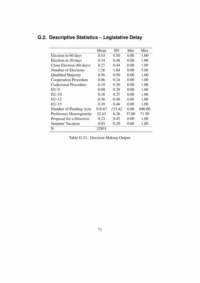
G.2. Descriptive Statistics – Legislative Delay

Mean SD Min MaxElection in 60 days 0.53 0.50 0.00 1.00Election in 30 days 0.34 0.48 0.00 1.00Close Election (60 days) 0.27 0.44 0.00 1.00Number of Elections 1.56 1.04 0.00 5.00Qualified Majority 0.56 0.50 0.00 1.00Cooperation Procedure 0.06 0.24 0.00 1.00Codecision Procedure 0.10 0.30 0.00 1.00EU-9 0.09 0.29 0.00 1.00EU-10 0.16 0.37 0.00 1.00EU-12 0.36 0.48 0.00 1.00EU-15 0.30 0.46 0.00 1.00Number of Pending Acts 510.67 133.42 0.00 696.00Preference Heterogeneity 52.63 6.26 37.80 71.50Proposal for a Directive 0.23 0.42 0.00 1.00Summer Vacation 0.04 0.20 0.00 1.00N 32891

Table G-21.: Decision Making Output.

71

G.3. Time Varying Coefficients for the MainEstimations

(1) (2) (3)60 days 30 days # Elections

Election -0.000** -0.000** -0.000**(0.000) (0.000) (0.000)

Cooperation Procedure 0.000** 0.000** 0.000**(0.000) (0.000) (0.000)

Codecision Procedure 0.001** 0.001** 0.001**(0.000) (0.000) (0.000)

Number of Pending Acts 0.000** -0.000 0.000*(0.000) (0.000) (0.000)

Preference Heterogeneity -0.000** 0.000* 0.000**(0.000) (0.000) (0.000)

Proposal for a Directive 0.000** 0.000** 0.000**(0.000) (0.000) (0.000)

Summer Vacation 0.000** 0.000** 0.000**(0.000) (0.000) (0.000)

Year FE Yes Yes YesObservations 32784 32784 32784Wald Test χ2 6790.76** 5946.60** 6586.52**

DV: Duration of Legislative ProcessSpecification: Nonproportional Cox Hazard Model

Standard errors in parentheses* p<0.10, ** p<0.05

Table G-22.: Time Varying Coefficients The models report coefficients of thetime-varying coefficients for the main estimations that are pre-sented in the book.

72

G.4. Electoral Delay Estimations for the Four Big EUCountries

Model 1 Model 2 Model 3 Model 4(Germany) (France) (UK) (Italy)

Election in 60 Days -0.417** 0.134** -0.210** -0.380**(0.029) (0.033) (0.038) (0.033)

Qualified Majority 0.457** 0.458** 0.461** 0.457**(0.021) (0.021) (0.021) (0.020)

Cooperation Procedure -1.128** -1.127** -1.126** -1.107**(0.044) (0.043) (0.043) (0.043)

Co-decision Procedure -0.997** -1.008** -1.016** -1.018**(0.041) (0.041) (0.041) (0.042)

EU-9 2.231** 2.163** 1.982** 1.826**(0.160) (0.161) (0.162) (0.161)

EU-10 1.421** 1.384** 1.270** 1.044**(0.129) (0.128) (0.129) (0.130)

EU-12 0.965** 0.841** 0.792** 0.613**(0.101) (0.102) (0.103) (0.104)

EU-15 0.354** 0.338** 0.324** 0.286**(0.071) (0.072) (0.071) (0.072)

Number of Pending Acts 0.003** 0.003** 0.003** 0.003**(0.000) (0.000) (0.000) (0.000)

Preference Heterogeneity 0.012** 0.011** 0.014** 0.016**(0.002) (0.002) (0.002) (0.002)

Proposal for a Directive -0.881** -0.886** -0.882** -0.889**(0.032) (0.032) (0.031) (0.031)

Summer Vacation -1.220** -1.239** -1.205** -1.200**(0.122) (0.122) (0.122) (0.122)

tvcElection in 60 Days 0.001** 0.000** -0.000**

(0.000) (0.000) (0.000)Cooperation Procedure 0.001** 0.001** 0.001** 0.001**

(0.000) (0.000) (0.000) (0.000)Co-decision Procedure 0.001** 0.001** 0.001** 0.001**

(0.000) (0.000) (0.000) (0.000)Number of Pending Acts -0.000 0.000 -0.000 -0.000

(0.000) (0.000) (0.000) (0.000)Preference Heterogeneity 0.000** 0.000** 0.000** 0.000**

(0.000) (0.000) (0.000) (0.000)Proposal for a Directive 0.000** 0.000** 0.000** 0.000**

(0.000) (0.000) (0.000) (0.000)Summer Vacation 0.000** 0.000** 0.000** 0.000**

(0.000) (0.000) (0.000) (0.000)Year FE Yes Yes Yes YesObservations 32784 32784 32784 32784Wald Test χ2 4090.707 4154.383 3903.157 4091.701



73

Model 1 Model 2 Model 3 Model 4(Germany) (France) (UK) (Italy)

Close Election in 60 Days -1.105** -0.232** -0.932** -1.160**(0.079) (0.039) (0.107) (0.074)




EU-9 2.344** 1.930** 2.082** 1.582**(0.162) (0.163) (0.159) (0.160)

EU-10 1.620** 1.288** 1.370** 0.829**(0.130) (0.129) (0.127) (0.129)

EU-12 1.114** 0.810** 0.909** 0.411**(0.103) (0.102) (0.101) (0.104)

EU-15 0.386** 0.321** 0.340** 0.320**(0.071) (0.072) (0.071) (0.072)



Proposal for a Directive -0.885** -0.886** -0.882** -0.884**(0.032) (0.032) (0.031) (0.032)

Summer Vacation -1.233** -1.257** -1.169** -1.158**(0.122) (0.123) (0.122) (0.121)

tvcCooperation Procedure 0.001** 0.001** 0.000** 0.000**

(0.000) (0.000) (0.000) (0.000)Co-decision Procedure 0.001** 0.001** 0.001** 0.001**

(0.000) (0.000) (0.000) (0.000)Number of Pending Acts 0.000 0.000 -0.000 -0.000**

(0.000) (0.000) (0.000) (0.000)Preference Heterogeneity 0.000** 0.000** 0.000** 0.000**

(0.000) (0.000) (0.000) (0.000)Proposal for a Directive 0.000** 0.000** 0.000** 0.000**

(0.000) (0.000) (0.000) (0.000)Summer Vacation 0.000** 0.000** 0.000** 0.000**

(0.000) (0.000) (0.000) (0.000)Close Election in 60 Days 0.001** -0.001** -0.001**

(0.000) (0.000) (0.000)Year FE Yes Yes Yes YesObservations 32784 32784 32784 32784Wald Test χ2 4074.05** 3898.61** 4141.36** 4521.58**



74

G.5. Additional Robustness – Legislative Delay

Model 1 Model 2 Model 3 Model 4(Directives) (Post 1990) (Size) (No TVC)

Election in 60 days -1.054** -1.022** -0.715** -0.877**(0.075) (0.028) (0.022) (0.019)




EU-9 1.495** 1.414**(0.382) (0.167)

EU-10 1.212** 1.259**(0.296) (0.135)

EU-12 0.891** 0.895** 0.737**(0.232) (0.112) (0.103)

EU-15 0.443** 0.471** 0.346**(0.171) (0.082) (0.075)



Proposal for a Directive -0.695** -0.853** -0.561**(0.042) (0.032) (0.022)

Summer Vacation -2.497** 0.122 -1.226** -0.882**(0.321) (0.155) (0.122) (0.070)

Number of EU Members -0.072**(0.006)

tvcElection in 60 Days -0.000** -0.000** -0.000**

(0.000) (0.000) (0.000)Cooperation Procedure 0.000** 0.000** 0.000**

(0.000) (0.000) (0.000)Co-decision Procedure 0.001** 0.001** 0.001**

(0.000) (0.000) (0.000)Number of Pending Acts 0.000** 0.000** 0.000**

(0.000) (0.000) (0.000)Preference Heterogeneity 0.000 -0.000** -0.000**

(0.000) (0.000) (0.000)Proposal for a Directive 0.000** 0.000**

(0.000) (0.000)Summer Vacation 0.000** 0.000** 0.000**

(0.000) (0.000) (0.000)Year FE Yes Yes Yes YesObservations 7490 17615 32573 32784Wald Test χ2 1200.13** 5172.64** 7013.71** 6516.00**



G.6. Do Governments Adjourn Adoptions until afterElections?

The empirical analysis in Chapter 8 provides evidence that governments in-deed aim to delay the adoption of legislative acts before national elections, but

75

the specification of the model does not allow us to analyze whether the delayindeed shifts the adoption of a proposal until after the election. If govern-ments successfully delay the adoption of legislative proposals, then one wouldexpect a decline in legislative output just before national elections. To analyzethis important question in greater depths, and to triangulate my argument aboutstrategic delay, I now analyze whether national elections reduce the amount oflegislative output before elections.

To test for electoral cycles in decision-making output, I aggregate the EULOdata set to count the number of legislative acts that are adopted in a givenmonth (Legislative Output (Month)). For the purpose of analysis I include alldecisions, regulations, and directives that were adopted by the EU. Figure G-21 presents the dependent variable graphically using box plots. On average,the EU adopts 38 proposals in a given month, but Legislative Output variesdramatically even within a 12-month period. Between 1976 and 2009, annuallegislative output varied between 0 and 168 acts. Legislative output peaks with168 acts which were adopted in December 2001.

I want to analyze whether the EU’s legislative output is affected by oppor-tunistic delay. My main independent variable is the election period. Since thelevel of analysis is not the proposal, but the month, I aggregate the electionindicators to the monthly level. Each month sees the adoption of about 39proposals, but most proposals are adopted at different days within each month.Consequently, some proposals within a given month fall within the 60 (or 30)days of an election while others do not. I calculate a variable that measures thenumber of proposals within each month that fall within 60 days (or 30 days)of a national election as share of total proposals within any given month. Thevariable Proposal, Election 60 days (%) takes values between 0 and 100, withan average of 3%. This implies that for some months there are no imminentelections for any of the proposals (value of 0), for some months all proposalsare close to elections (value of 100), and on average about 3% of proposals inany given month are close to national elections. The average number of pro-posals affected by elections is lower when we calculate the same variable forelections that are 30 days apart (the average share of proposals is 2.6%).

If national elections really lead to a delay of legislative adoptions until afterthe elections, we should observe that the number of adopted proposal is lowerbefore national elections and higher after national elections. The data structuredoes not allow me to test a direct post-election effect, but I can analyze whetherthe average number of days to the next election for proposals within a given

76

0 50 100 150 200Number of Acts Adopted

2009200820072006200520042003200220012000199919981997199619951994199319921991199019891988198719861985198419831982198119801979197819771976

Figure G-21.: Tides in Legislative Output in the EU, 1976-2009. The graph de-picts box plots of the number of legislative acts adopted in each month be-tween 1977 and 2009. Source: EULO and own calculations.

77

month has an effect (Time to Next Election (avg)). I would expect that thefurther away the next election, the greater the number of legislative adoptions.

I also add a number of control variables to the model estimations, follow-ing previous work (Leuffen, 2008; Hertz and Leuffen, 2011). QMV (#) codesthe number of proposals that are decided with qualified majority voting eachmonth. According to previous research, QMV procedures should expeditedecision-making; the more proposals are decided by majority in a given month,the less able EU governments to veto decisions until after the election. I furtherinclude dummy variables to test for the effect of enlargements from the EU-9to the EU-25. Directives (#) counts the number of proposals that are pendingdirectives in each month, and Acts Pending (#) counts the average number ofacts that are pending in the legislative process in any given month. August isa dummy variable that takes the value 1 for the month of August, when mostEuropean politicians are on vacation. Cooperation (#) and Co-decision (#) arethe number of proposals that are decided under the cooperation and codeci-sion procedure in each month, respectively. Finally, I include a variable onthe heterogeneity of EU member state preferences (Hertz and Leuffen, 2011),which analyzes the range of all government positions in the Council, based ona left-right dimension.

Table G-23 presents the main results of a negative binomial event countregression with year fixed effects. Model 1 is the main model which includesProposal, Election 60 days (%), that is the share of proposals that fall within 60days of an election in any given month. Model 2 analyzes whether Time to NextElection (avg) has a positive effect on legislative output, and Model 3 replacesthe main election indicator with an indicator of the proportion of proposalswithin a given month that fall within 30 days of an election (Proposal, Election30 days (%)). The models fit the data well. Using the Wald test, I can rejectthe null hypothesis that the coefficients are jointly equal to zero.

All election variables have the expected effect. The number of adopted leg-islative acts in any given month decreases when elections are upcoming atthe national level. In particular, the coefficient indicates that as the share ofproposals that are negotiated close to elections increases in any given monthso does the number of adoptions decrease. The effect is negative for bothelection indicators in Models 1 and 3. The interpretation of coefficients in anegative binomial event count regression is not straightforward, so I displaythe marginal effect of Proposal, 60 Days Before Election (%) graphically. Fig-ure G-22 graphs the predicted legislative output in each month for different

78

Model 1 Model 2 Model 3 Model 4Proposals Within 60 Days of Election (%) -0.051**

(0.010)Time to Next Election (avg) 0.001**

(0.001)Proposals Within 30 Days of Election (%) -0.034**

(0.006)Proposals Within 60 Days of Close Election (%) -0.041**

(0.005)QMV (#) 0.011** 0.012** 0.011** 0.009**

(0.001) (0.001) (0.001) (0.001)9 Members 0.292 -0.632** -0.246 0.752**

(0.394) (0.309) (0.228) (0.237)10 Members -0.081 -0.160 -0.134 0.050

(0.177) (0.195) (0.183) (0.199)12 Members -0.275* -0.347** -0.382** -0.335**

(0.155) (0.167) (0.163) (0.142)15 Members 0.452 0.476 0.692* 0.375

(0.363) (0.407) (0.392) (0.344)Directive (#) -0.003* -0.003 -0.003* -0.002

(0.002) (0.002) (0.002) (0.002)Acts Pending (#) 0.000 -0.000 0.000 0.000

(0.000) (0.000) (0.000) (0.000)Codecision (#) -0.009** -0.011** -0.011** -0.007**

(0.003) (0.003) (0.003) (0.003)Cooperation (#) -0.003 -0.004 -0.003 -0.003

(0.004) (0.004) (0.004) (0.005)August -1.005** -1.917** -1.462** -1.174**

(0.201) (0.133) (0.259) (0.222)Preference Heterogeneity 0.006 0.010 0.006 0.001

(0.008) (0.008) (0.008) (0.017)Constant 3.007** 2.876** 3.070** 3.294**

(0.468) (0.525) (0.477) (0.893)Year Fixed Effects Yes Yes Yes YesObservations 333 369 317 210Pseudo R2 0.155 0.144 0.144 0.152Wald Test χ2 887.682 711.456 747.849 786.825

DV: Number of Legislative Acts Adopted (Month)Standard errors in parentheses

* p<0.10, ** p<0.05

Table G-23.: Elections and Decision-Making Output. The models report coeffi-cients of a negative binomial event count model with year fixed effects.

79

values of my main explanatory variable, holding all other variables constant.The effect of national elections is sizable: The EU adopts about 46 proposalseach month if none of these proposals fall within an electoral period. Thisnumber falls to 39 proposals if 3% of proposals fall 60 days before nationalelections (the sample average). If 20% of proposals that are in the legislativeprocess in a given month fall within an electoral period, then legislative outputfalls to 4 proposals. If all proposals fall within an electoral period, the modelpredicts that not even one proposal would be adopted in that month, though thechange in marginal effects is insignificant if more than 60% of proposals arenegotiated during an election period. Note, however, that most observationsfor Proposal, 60 Days Before Election fall between 0% and 9%. We wouldtherefore expect a decrease in legislative output by between 6 and 18 propos-als, on average. This effect is rather large given that the average number ofproposals that are adopted each month is 39.

For Election (30 days), the effect is slightly smaller: Holding all other vari-ables constant, the EU adopts about 46 proposals in a month when no proposalis close to a national election, to about 23 proposals if 20% of them fall in anelection period, and only about 2 proposals if all proposals are close to elec-tions. The marginal effects for Time to Next Election (avg) can provide furtherinformation about the post-election period. The longer the time until the nextelection the greater the legislative output in any given month. The variableranges from 9 to 308 days, with an average of 82 days. We are most interestedin periods where the time to the next election is very long. For example, ifelections are about 110 days away, on average, then the EU adopts about 44proposals each month, more than the 39 proposals during the 60 day electionperiod window. If elections are over 300 days apart then EU members adoptmore than 57 proposals each month.

The decline in legislative output is partially compensated in periods whereno elections occur, but as the findings indicate, elections lead to a total de-cline in legislative output. Turning to the control variables, the more proposalsare decided by qualified majority, the greater the legislative output. Regula-tions are more likely to be adopted in a timely fashion than other acts, andthe month of August sees very few adoptions. The codecision procedure alsoreduces legislative output. And whereas the enlargements of the 1980s de-creased legislative output, there has been no effect in subsequent enlargementrounds.

In sum, national elections lead to a delay in the adoption of individual pro-

80

01

02

03

04

05

0P

red

icte

d N

um

be

r o

f A

do

pte

d P

rop

osa

ls

0 10 20 30 40 50 60 70 80 90 100Proposals Within 60 Days of Election (%)

Figure G-22.: Elections and Legislative Output. The graph displays marginal effectsof Proposal, 60 Days Before Election (%). It graphs the predicted legisla-tive output in each month (y-axis) for different values of Proposal, 60 DaysBefore Election (%) (x-axis), holding all other variables constant.

81

posals until after the election, and they have a significant effect on legislativetides in the European Union. Even controlling for a number of important de-terminants of legislative activity, elections can have a detrimental effect on thelikelihood that decisions are reached in a timely fashion. The operationaliza-tion of the variable Proposals, 60 Days Before Election (%) allows us to shedmore light on the effect of elections on legislative activity. It indicates thatas the proportion of proposals that are negotiated closely before an election inany given month increases, legislative output decreases. The more proposalsare negotiated before elections, the greater the effect of elections on legislativetides.

H. Appendices for Chapter 9 (The WaitingGame)

H.1. Two Alternative Explanations – Delay Case StudyIn the case study, I argue that Angela Merkel’s decisions during the Greek debtcrisis were motivated by electoral considerations. There are, however, twocommon alternative explanations of her behavior that I would like to address.The discussion is taken from Schneider and Slantchev (2017).

A Policy Blunder?One possible explanation interprets the delay as a failure of German politiciansto see past the cultural and ideological commitment to austerity, and a failureto understand how financial markets could spread the Greek malady to othervulnerable members of the Eurozone. As the former foreign minister JoschkaFischer put it, Merkel had made such a “complete mess” of the crisis that hecould “not think of a situation since 1949 that [had] been handled so badly”?5

Whereas the cultural affinity to austerity policies and the popular fear of infla-tion certainly did not make it easier for the German government to commit toa bailout, there are two problems with this explanation.

First, it requires one to maintain that Merkel had been singularly deludedwhen other governments, the EU Commission, and the IMF were all in agree-

5The Independent. May 23, 2010. “Euro crisis is melting support for ‘Iron’ Merkel.”

82

ment that the Greeks needed a bailout. European leaders urged Merkel notto delay the bailout to Greece, but to act in solidarity with other members ofthe Eurozone. Italian Foreign Minister, Franco Frattini, pointedly stated thatthere was a “moral duty to intervene as soon as possible.”6 It is difficult to seehow Merkel and her ministers could have been so out of touch with marketreality, especially in late April when they still maintained that Germany couldrefuse to aid Greece. In a highly critical article, Professor Horn argued thatit had been foreseeable that the failure to provide unambiguously a backstopfor Greece would incite further speculation, which would drive up the priceof government bonds, making it impossible for the country to refinance itselfthrough the markets despite the austerity measures.7 In other words, the Ger-man government’s “dive-like” behavior, its “submissiveness to the financialmarkets and its cowardice towards the tabloid press” brought about the veryoutcome it had been supposedly trying to prevent: a Greek bailout.

Moreover, if the German government did not care about Greeks, it pre-sumably did care about the investments of German banks, whose exposureto Greece in the first quarter of 2010 was, at $44.2bn (24% of the total ex-posure of European banks), second only to France’s $71.1bn.8 As Alessan-dro Leipold, former acting director of IMF European department, noted, therewere “intrinsically strong German interests” at stake.9 There is no doubt thatthe German government was aware of these highly risky entanglements.10 Itis very implausible that it would not have acted upon this knowledge to pre-vent an almost certain spillover of the crisis to Germany just because of itscultural commitment to austerity; especially since this would have almost in-evitably created the inflationary pressures that the government was determinedto prevent.

Second, and crucially, the explanation cannot account for the clobbering

6Agence France Presse. March 22, 2010. “EU ups pressure on Merkel to aid Greece.”7Spiegel, “Hesitation and Patronizing Advice: How Germany Made the Greek Crisis Worse”,

April 27, 2010.8Buiter and Rahbari (2010, Figure 4), http://willembuiter.com/Greece.pdf,

accessed May 9, 2016.9New York Times, “Already Holding Junk, Germany Hesitates”, April 28, 2010. The German

Hypo Real Estate Holding held $10.5bn of Greek debt, and since it was owned by thepublic after its own bailout in 2009, it was German taxpayers whose money was on theline.

10Not only did the German government know; it had already secretly acted upon these risksby providing bailouts to its entangled banks in 2008 and 2009 (Bastasin, 2012).

83

http://willembuiter.com/Greece.pdf

the voters in NRW delivered to Merkel’s party. Suppose that the Chancellorhad been just as convinced as the voters of the wisdom of the schwabischeHausfrau strategy until the end of April but then underwent a rapid conversion.If Merkel had such a “road to Damascus” moment, then it is by no means clearwhy she could not have persuaded the voters of the wisdom of her new policy.After all, she had been the most hawkish Eurozone leader on Greece, and ifshe had suddenly come to the realization that a bailout was necessary to savethe euro, the voters should have believed her. Only Nixon could go to China,and only Merkel could go to Greece. But the voters did not believer her. . . orelse how does one explain CDU’s abysmal performance at the polls?

One might be tempted to argue that the German voters punished the CDUbecause Merkel was inconsistent — first opposing the bailout, but then flip-flopping — or because her Machiavellian tactics had worsened the crisis, sad-dling Germany with six times the costs. Commenting on the fact that providingthe bailout must have been obviously inevitable to Merkel, Tagesspiegel put itclearly:

The Chancellor, the master tactician, lacked the self-confidenceand courage to follow her instincts and respond quickly to the cri-sis.11

Jurgen Rutters, the Premier Minister of NRW, blamed the national govern-ment for its handling of the financial crisis.12 Senior figures in the CDU openlysaid that they had lost confidence in Merkel’s ability to lead and called on herto quit.13

This, however, was not how the Germans voters interpreted it. They re-mained unconvinced about the seriousness of the crisis. Polls in late April andearly May showed that the majority of Germans opposed the bailout becausethey believed it was wrong to aid Greece. Surveys also revealed that they didnot consider the crisis a top priority for Germany, and did not expect it to af-fect them adversely personally. These data point to a failure to carry the voterson the new policy, not to a punishment for not dealing with a serious crisispromptly.

11Der Tagesspiel. May 10, 2010. “Fur die Regierung Merkel geht es ums Uberleben.”12The Times. May 10, 2010. “Poll blow for Merkel amid anger over Greek bailout.”13Daily Telegraph. May 11, 2010. “Calls for Merkel to quit over Greek bailout.”; The Times.

May 12, 2010. “Wounded Merkel’s star fades amid acrimony and intrigue.”

84

Since they did not consider a Greek bailout necessary, the volte-face of theruling coalition was seen as wasting taxpayer money on foreigners when itwas needed at home. As Ingrid Lange, a shop assistant from NRW, put it in astatement that described the general interpretation,

First the state had to rescue the banks and now they have to rescueGreece when our own economy is suffering. It’s hard to make adecent living even with a job. The government should spend ourtaxes where they’re needed.

This suggests that Merkel and the CDU lost not because they were blamed fornot acting fast enough or because she had pursued an inconsistent strategy, butbecause the voters in NRW still believed that a Greek bailout was inappropri-ate.

At the beginning of this section, I cited Joschka Fischer, who delivered theblunt and unflattering verdict that Merkel had made a “complete mess” of thecrisis. It is worth asking, however, what the alternative could have been. Sincedelaying after the credit downgrades seems to have been out of the question,the only plausible road not taken must have been acting sooner. With thepriors of German voters strongly fixed against the seriousness of the crisis,this would have resulted in an electoral punishment at least as bad as the onethat actually happened. In fact, without Merkel holding the line in the faceof serious criticism by other Eurozone members, the slide in public opinionpolls would have continued. It is also arguable that had Merkel jumped onthe bailout bandwagon early on, it would have been even more difficult forvoters to believe that the action had been warranted. The delay deepened thecrisis so much that even the massive bailout proved insufficient to stabilizethe Eurozone. Ironically, by allowing the consequences to reveal themselves,Merkel probably made it possible for Germany to participate fully in the sub-sequent two bailouts. Thus, the unfortunate downgrades and the panic theycaused triggered the drastic reversal that made a mockery of the otherwisesolid strategy Merkel had been playing. To her credit, however, when it be-came clear that further inaction would cause grave harm to the German econ-omy, Merkel abandoned the electorally-motivated strategy to do the right thingdespite knowing full well that the voters would not see it that way.

85

A War of Attrition?A second possible explanation centers around a potential distributional con-flict as the source for the delay. Accordingly, Merkel was holding out forbetter terms, both from the Greek government and from the fellow Eurozonemembers. The former had to commit to even more drastic austerity measures,while the latter had to agree to terms that would not prejudice the credibility ofthe threat to let future spendthrifts sort out their own problems. The peculiarinsistence on IMF participation — long opposed by other Eurozone members— must be seen in that light, as that organization had a lot of experience ofimposing unpopular reforms on recipient countries.14

The Chancellor defended herself by arguing that her government had to holdout for satisfactory terms, but that the “last resort” had been reached. It nowhad to act to save the euro, which was the foundation of German prosperity,and whose collapse would have incalculable consequences for Europe and be-yond. As she put it,

The price of our attitude was to be criticized for being hesitant orbeing slow. But such a price, ladies and gentlemen, the federalgovernment will gladly pay if it ensures the right decision in theend.15

Let us set aside the fact that from a political perspective this was the onlyargument Merkel could have advanced in her defense: she could neither ownup to a colossal mistake nor fess up to a misfired electoral ploy.

The war of attrition logic can certainly contribute to explain the initial phaseof negotiations. As the crisis worsened in early 2010, Greece was increas-ingly willing to accept tougher austerity measures as demanded by the Germangovernment. The problem with this explanation is that Germany had alreadyachieved all of its stated goals in principle with the March 25 agreement, andin practice with the April 11 decision to make the rescue mechanism fullyoperational.16 The IMF had been involved since the March agreement, and14The was not about the distribution of costs amongst the creditors. Each EU member’s

contribution to a bailout were pre-determined by the ECB key.15Bundesregierung, “Regierungserklarung von Bundeskanzlerin Merkel zu den Euro-

Stabilisierungsmaßnahmen,” May 19, 2010.16Spiegel Online, “ The Greek Bailout Plan: Merkel’s Risky Hand of Brussels Poker”, March

26, 2010. Spiegel, “An Aid Package in the Billions: Merkel’s Bluff Called in Poker overGreece,” April 12, 2010.

86

Schauble himself had indicated in an interview that the outline of the auster-ity program had been decided in mid March.17 Moreover, Merkel had alreadydropped the insistence on market rates for the loans in the April 11 agreement.As Frank Schaffler, the deputy finance spokesman for Merkel’s coalition part-ner FDP, characterized it at the time, “Germany buckled under the pressure –we shouldn’t kid ourselves that such loans are anything but subsidies.”18 Fi-nally, Bastasin (2012, 70) explains how the “shallow text” of the February 11agreement, with its emphasis on the defense of the stability of the monetaryunion, had been a “crucial strategic coup for Merkel” because it allowed herto deflect a potential bailout challenge by the Constitutional Court.

While it is true that the Greek government announced a third wave of cutsin conjunction with the May 2 deal, one cannot argue that Merkel had delayedto obtain its formal commitment. The Chancellor herself claimed to havedone so because without Athens announcing new austerity measures, givingaid “would have had the opposite effect” to calming markets.19 The irony ofthis statement in light of the reason the markets had gone berserk cannot beoverstated.

In fact, it was because of this that the press and the opposition had specu-lated that Merkel’s tough line had been a domestic kabuki theater at least sinceMarch.20 That is also why Steinmeier, accused Merkel of playing a doublegame between Brussels and Berlin, “Madame No – that was a huge hoax.”21

He also dismissed the notion that the delay had been a part of some coherentplan to create a better policy. As he told Merkel, “You drifted around like awindsock. Then in retrospect you call that your strategy. Your double gamehas cost us an enormous amount of trust and respect in Europe.”22 The alle-gation of ex post rationalization is also supported by the fact that the Germangovernment only belatedly (after April 28) started to insist on the importanceof the crisis for Germany itself.

This explanation also has a flaw in the logic of the strategy itself given thatit was being played in an electoral shadow. Merkel could have denied thatthe Greek crisis posed a problem for Germany in an attempt to signal that her

17Deutschlandfunk April 22, 2010.18Bloomberg, “Germany Says Greek Aid Probably Needs Parliament Vote,” April 14, 2010.19Agence France Presse, “Merkel defends foot-dragging over Greece,” May 5, 201020Rheinische Post, “Heute geht es auch um Merkels Zukunft,” May 8, 2010.21XN Press, “Steinmeier: Nur Geld uberweisen, reicht nicht,” May 3, 2010.22Agence France Presse, “Merkel defends taking time over Greece,” May 5, 2010.

87

government had little incentive to act unless all its stringent conditions hadbeen met. This might have increased the credibility of the threat, but sinceshe had done it so publicly, it also signaled to the German electorate that abailout was unnecessary. Judging from the opinion surveys and the prevalentopinion in the press, the voters seem to have believed her. But if Merkel knewa bailout was coming and was merely stalling for terms, this would have beena silly thing to do because the bailout would certainly upset the voters. A moreprofitable strategy would have been to indicate that a bailout was necessary andoutline the conditions Athens had to satisfy to obtain it. Of course, Merkel laterclaimed that this had been precisely what she had done, except that somehownobody had understood her that way: not the IMF, not her fellow Europeanheads of state, not the domestic opposition, not the press, and not the voters.23

23Spiegel, “ German Finance Minister Wolfgang Schauble: ’We Cannot Allow Greece to Turninto a Second Lehman Brothers’,” April 19, 2010.

88

BibliographyAitchison, John. 2003. The Statistical Analysis of Compositional Data. Cald-

well: Blackburn Press.

Aksoy, Deniz. 2010. “Who Gets What, When, and How Revisited: Votingand Proposal Powers in the Allocation of the EU Budget.” European UnionPolitics 11(2):171–194.

Aksoy, Deniz and Jonathan Rodden. 2009. “Getting into the Game: LegislativeBargaining, Distributive Politics, and EU Enlargement.” Public Finance andManagement 9(4):613–643.

Bastasin, Carlo. 2012. Saving Europe: How National Politics Nearly De-stroyed the Euro. Washington, D.C.: Brookings Institution Press.

Box-Steffensmeier, Janet M and Christopher Zorn. 2001. “Duration Modelsand Proportional Hazards in Political Science.” American Journal of Politi-cal Science 45(3):951–67.

Box-Steffensmeier, Janet M., Dan Reiter and Christopher Zorn. 2003. “Non-proportional Hazards and Event History Analysis in International Rela-tions.” Journal of Conflict Resolution 47(1):33–53.

Buiter, Willem H. and Ebrahim Rahbari. 2010. “Greece and the fiscal cri-sis in the EMU.”. Working paper, Citi Investment Research and Analysis,September 7, 2010.

Dassonneville, Ruth and Marc Hooghe. 2017. “Economic Indicators and Elec-toral Volatility. Economic Effects on Electoral Volatility in Western Europe,1950-2013.” Comparative European politics 15(6):919–943.

Doring, Holger and Philip Manow. 2015. “Parliaments and Governmentsdatabase (ParlGov): Information on Parties, Elections and Cabinets in Mod-ern Democracies.” Development Version.

89

Golub, Jonathan and Bernard Steunenberg. 2007. “How Time Affects EUDecision Making.” European Union Politics 8(4):555–566.

Grambsch, PM and TM Therneau. 1994. “Proportional Hazards Tests andDiagnostics Based on Weighted Residuals.” Biometrika 81(3):515–526.

Hertz, Robin and Dirk Leuffen. 2011. “Too Big to Run? Analyzing the Impactof Enlargement on the Speed of EU Decision-Making.” European UnionPolitics 12(2):193–215.

Leuffen, Dirk. 2008. “Ever More Complex? Domestic Politics in the EnlargedEuropean Union.” Unpublished Working Paper.

Rodden, Jonathan. 2002. “Strength in Numbers? Representation and Redistri-bution in the European Union.” European Union Politics 3:151–175.

Schmitt, Hermann, Evi Scholz, Iris Leim and Meinhard Moschner. 2005. “TheMannheim Eurobarometer Trend File, 1970-2002 [Computer file].” Pre-pared by Zentralarchiv fur Europaische Sozialforschung und Zentrum furUmfragen, Methoden und Analysen.

Schneider, Christina J. 2013. “Globalizing Electoral Politics: Political Compe-tence and Distributional Bargaining in the European Union.” World Politics65(3):452–490.

Schneider, Christina J. and Branislav L. Slantchev. 2017. “The Domestic Pol-itics of International Cooperation. Germany and the European Debt Crisis.”International Organization 72(1):1–31.

90

Date post:	23-Mar-2022
Category:	Documents
Upload:	others
View:	2 times
Download:	0 times

Appendix - University of California, San Diego

Documents