Appl. Note, Active Antennas for Radiomonitoring · PDF fileActive Antennas for Radiomonitoring...

Active Antennas for Radiomonitoring Application Note

Products:

Generally applicable to all active antennas from Rohde & Schwarz,

in particular this Application Note covers the following products:

ı R&S®HE600

ı R&S®HE010E

ı R&S®HE010D

ı R&S®HE016

ı R&S®HK014E

ı R&S®HL033

ı R&S®IN600

The fundamental working principles of active antennas are asserted and it is described what makes them

different compared to passive antennas. Furthermore the important parameters relating to active antennas

are explained and typical system applications are discussed - including a comparison with passive antenna

solutions and a chapter explicitly dealing with radio monitoring in the HF frequency range.

Note:

Please find the most up-to-date document on our homepage

http:\\www.rohde-schwarz.com/appnote/8GE02

App

licat

ion

Not

e

Mai

k R

ecke

weg

2.20

16 –

8G

E02

_0e

http://www.rohde-schwarz.com/appnote/8GE02

http://www.rohde-schwarz.com/appnote/8GE02

Introduction

8GE02_0e Rohde & Schwarz Active Antennas for Radiomonitoring

2

Table of Contents

1 Introduction ......................................................................................... 3

2 Working principles.............................................................................. 4

3 Characteristics of active antennas .................................................... 6

3.1 Antenna Impedance ..................................................................................................... 6

3.2 Antenna factor .............................................................................................................. 7

3.3 Antenna noise .............................................................................................................. 8

3.4 Sensitivity ...................................................................................................................10

3.5 Gain .............................................................................................................................11

3.6 Non-linear distortion..................................................................................................12

3.7 Dynamic range ...........................................................................................................13

4 Application examples ....................................................................... 15

4.1 Calculation of field strength in the far field ............................................................15

4.2 VHF example scenario ..............................................................................................16

4.2.1 Scenario 1 - Reception of a weak signal .....................................................................16

4.2.2 Scenario 2 - Reception of a weak signal in the presence of strong interference ........20

4.2.3 Other measures to reduce or avoid intermodulation ...................................................25

4.3 HF example scenario .................................................................................................26

4.3.1 Effects on polarization caused by the ionosphere .......................................................26

4.3.2 Field strength measurement at HF using different types of antennas .........................26

4.3.3 Selecting an appropriate HF antenna ..........................................................................29

4.3.4 Active HF monitoring antennas summarized ...............................................................32

5 Literature ........................................................................................... 33

6 Glossary ............................................................................................ 34

Introduction


3

1 Introduction

The usage of active antennas for radio monitoring purposes is nowadays well

established. This is due to good reason. When it comes to broadband capabilities and

significant size reduction, there is no better solution than an active receiving antenna.

Care must only be taken when the active antenna is used at locations where very high

field strength values are present. But even then, problems tend to occur mainly due to

improper installation and not by reason of the active antenna itself.

Active antennas employ optimum matching of the passive radiator(s) to the active

electronic circuit. Consequently the function of the radiator(s) and the electronics can

no longer be described independently - like it is possible for a passive antenna with a

preamplifier. This application note starts with a fundamental description of the working

principle of active antennas. Furthermore it explains their characteristic parameters

which should help the reader to decide if an active antenna is appropriate for a certain

application. Typical application examples will aid to the understanding here.

Working principles


4

2 Working principles

By definition an active antenna contains at least one active component (e.g. a field

effect transistor) which is installed in immediate vicinity of the radiator(s) of the

antenna. The purpose of this active component is primarily to match the impedance of

the electrically short radiator (or pair of radiators) to the nominal impedance (i.e. 50 Ω).

A careful selection of the active device allows reasonable matching over a very wide

range of input impedances and thus allows the design of an active antenna with a very

broad frequency bandwidth.

Figure 1 shows the principal build-up of an active monopole antenna.

Figure 1: Concept of an active monopole antenna

To understand the fundamental working principle of an active antenna, two physical

phenomena must be visualized:

ı The quality of reception (of a signal of interest) is not only determined by the

signal voltage measured with a connected receiver, but predominantly by the ratio

of the signal level compared to the noise level present at the output of the receiver

- the so-called Signal-to-Noise Ratio (abbreviated S/N or SNR).

ı The signal voltage that can be measured at the output of a radiator (or a pair of

radiators) will depend on the field strength present at the location of the antenna -

or to be more precise, on the field strength vector which matches the polarization

of the antenna - and on the physical dimensions of the antenna itself. An

acceptable approximation here is that for a given constant field strength, the

voltage is proportional to the length of the antenna.

Working principles


5

Figure 2: Fundamental working principle of S/N versus antenna length

Obviously the active antenna cannot differentiate between the wanted signal and the

noise that arrives at the antenna simultaneously. Figure 2 shows on the left side that if

the antenna length is reduced, the wanted signal (PS) and the noise (PN) picked up

from the environment are reduced by the same amount. This leads to a constant

Signal-to-Noise Ratio (S/N) as shown on the right side. So the quality of reception does

not suffer.

However the reduction of radiator length cannot be driven to extremes. As soon as the

received noise (PN) picked up from the environment reaches the order of the internally

generated noise of the receiver (PE) the S/N will be reduced.

Hence, the optimum length of a radiator is depending on the noise figure of the

receiver as well as on the environmental noise present at the antenna location.

According to [2] there are different contributions to the environmental noise as shown

in Figure 3. For the majority of the HF frequency range the man-made noise is

dominating, together with contributions from atmospheric and galactic sources. Man-

made noise strongly varies with location and is worst for city locations.

Figure 3: Different sources of environmental noise versus frequency compared to the theoretical

minimum noise level

Antenna length Antenna length

S / N

P

PS

PN

PE

P

PS

PN

PE

Antenna length

S/N

Characteristics of active antennas


6

3 Characteristics of active antennas

3.1 Antenna impedance

As mentioned in [1], the antenna input impedance depends strongly on the antenna

length. Figure 4 shows the equivalent circuit of an antenna where

UOC is the open circuit voltage at the antenna terminals

RL is the loss resistance of the antenna

Rr is the radiation resistance of the antenna

Xa is the antenna reactance and

Z0 is the receiver (and cable) impedance (nominal 50 Ω)

Figure 4: Equivalent circuit of an antenna

At resonance (i.e. radiator length of approx. λ/2 for a dipole) the antenna reactance Xa

becomes zero and the antenna impedance is purely resistive.

But as active antennas usually feature electrically short radiators (radiator length << λ)

the radiation resistance Rr and the loss resistance RL can be neglected and the major

contribution for the impedance is due to the radiator reactance Xa.

The result is a total mismatch between radiator impedance and the nominal impedance

Z0, assuming that the radiator is directly connected to the nominal impedance of the

cable or the receiver.

If an active circuit (i.e. a field effect transistor) is directly located at the radiator(s) of the

antenna it can match the high radiator impedance (in terms of magnitude) to the low

nominal impedance Z0. So the main task of the active device is impedance

transformation rather than amplification of the signal. This results in an impedance of

Z ≈ 50 Ω at the antenna connector.

Figure 5 shows the impedance characteristics of a 1 m long rod (monopole antenna)

for the frequency range from 1 MHz to 200 MHz. The capacitance Ca is equal to

approx. 14 pF. For frequencies up to approx. 30 MHz the reactance of Ca dominates

the antenna impedance. The first resonance (λ/4) is visible at approx. 70 MHz where

Xa equals zero and a second resonance (λ/2) can be found at approx. 125 MHz.



7

Figure 5: Impedance characteristic of a 1 m long rod (or monopole) antenna

3.2 Antenna factor

Like for passive antennas, the antenna factor (or also called transducer or conversion

factor) is defined as the ratio of incident electric field strength Ei and the output voltage

of the antenna at its load impedance

𝐾 =𝐸𝑖

𝑈𝐿

(1)

The small signal equivalent circuit of an active antenna with an electrically short

radiator using a field effect transistor (FET) in common source configuration is shown

in Figure 6.

Figure 6: Small signal equivalent circuit of an active antenna

If the influence of the gate-drain capacitance Cgd and the conductance Ggs and Gds are

neglected the voltage at the load UL can be calculated with the simplified formula

𝑈𝐿 ≈−𝑔𝑚

𝐺𝐿

𝐶𝑎

𝐶𝑎 + 𝐶𝑔𝑠

𝑈𝑂𝐶 (2)

length in λ



8

As already mentioned in chapter 2, the open circuit voltage UOC is proportional to the

antenna length heff

𝑈𝑂𝐶 ≈ 𝐸𝑖 ℎ𝑒𝑓𝑓 (3)

Consequently the antenna factor can be approximated with the formula

𝐾 = 𝐸𝑖

𝑈𝐿

= 𝐺𝐿(𝐶𝑎 + 𝐶𝑔𝑠)

𝑔𝑚 𝐶𝑎 ℎ𝑒𝑓𝑓

= 𝑐𝑜𝑛𝑠𝑡 (4)

The formula shows that the antenna factor K is almost constant over a wide frequency

range. This can also be seen in Figure 7 which shows the typical antenna factor versus

frequency for the R&S®HE010E active rod antenna.

Figure 7: Typical antenna factor of R&S®HE010E active rod antenna

3.3 Antenna noise

While the active circuit directly at the antenna is able to match the impedance of the

short radiator(s) to the nominal impedance Z0 , it also adds a certain amount of noise to

the output of the circuit which will affect the noise figure of the antenna.

As an example Figure 8 shows the basic equivalent circuit of a junction field effect

transistor (JFET) in common source configuration identifying the equivalent noise

sources en and in that can be calculated with an appropriate FET model. While the

noise voltage en is independent of the source impedance, the noise current in is directly

depending on the source impedance Za.

JFET type transistors are preferred for active antenna applications due to their

inherently lower noise current in compared to bipolar devices [4].

Note that active antennas can also utilize other types of active devices or other

amplifier configurations, e.g. common drain or common gate. For simplicity reasons the

noise and antenna factor calculations here are based on the JFET common source

circuit.



9

Figure 8: Noise model of a junction FET transistor

According to [3] the noise factor of a noisy two-port (i.e. an active antenna) can be

calculated with the formula

𝐹𝑎 = 1 +𝑒𝑛

2 + |𝑍𝑎2|𝑖𝑛

2 + 2 𝑅𝑒(𝑒𝑛𝑖𝑛∗ 𝑍𝑎)

4𝑘𝑇0𝐵 𝑅𝑒(𝑍𝑎) (5)

where en and in are the before mentioned equivalent noise sources and Za is the

antenna impedance.

If again a 1 m long rod antenna with an impedance curve as shown in Figure 5

connected to a JFET circuit in common source configuration is assumed, the equation

above will be dominated by the magnitude of the antenna impedance and the

corresponding noise figure of such an antenna is shown in Figure 9.

Figure 9: Noise figure of a 1 m long active rod antenna with JFET common source configuration

Note that noise figure NF and noise factor F are related via the formula:

𝑁𝐹 = 10 log (𝐹) (6)

So essentially the matching of the short rod antenna to the nominal impedance Z0 is

causing a largely increased noise figure. Of course the antenna impedance can be

chosen to give the lowest possible noise figure, but as can be seen in Figure 9 this is

only possible for a very narrow frequency range.



10

3.4 Sensitivity

Based on the noise factor Fa it is possible to calculate the sensitivity of an active

antenna Emin. This parameter, which is also referred to as the field strength

sensitivity, indicates the minimum field strength value an antenna can detect in a

certain bandwidth. It is calculated with the formula

Emin =1

λ √

4π Z0k T0B Fa

D (7)

where

Z0 is the impedance of free space (≈ 377 Ω)

k is Boltzmann's constant (1.38 x 10-23 J/K)

B is the bandwidth in Hertz and

D is the directivity of the passive radiator

In a practical application it may be more convenient to use the logarithmic formula

𝐸𝑚𝑖𝑛 = −96.8 𝑑𝐵µV/m + 20 log (𝑓

𝑀𝐻𝑧) + 10 log (

𝐵

𝐻𝑧) +

𝑁𝐹𝑎

𝑑𝐵−

𝐷

𝑑𝐵 (8)

The field strength sensitivity of an active antenna always has to be seen in the context

of the environmental noise. This is especially important at LF, MF and HF frequencies

where the environmental noise level is usually high. Figure 10 shows the field strength

sensitivity of the R&S®HE010E active rod antenna compared to the theoretical

minimum field strength sensitivity (blue curve). This theoretical curve has been

determined based on the environmental noise curves from Figure 3 where a quiet

rural location is assumed. If the antenna is installed in a residential area where higher

levels of man-made noise are usually present (red curve), it can be seen that the

inherent noise of R&S®HE010E is almost equal or even below those values.

Figure 10: Field strength sensitivity of R&S®HE010E compared to the theoretical minimum and to the

man-made noise in a residential area.

Theoretical minimum

Man-made noise (residential)

R&S HE010E



11

Consequently a further reduction of the antenna noise figure does not lead to a

perceivable improvement of sensitivity in such surroundings

If the antenna noise factor Fa is equal to the external noise factor Fex, the overall S/N

ratio is degraded by 3 dB.

The sensitivity of an active antenna is normally specified for the antenna alone.

However as already mentioned the antenna must be seen not only in the context of the

external noise but also in the overall system. In combination with a receiver, the

system noise factor FS can be calculated in order to determine the overall system

sensitivity.

𝐹𝑆 = 𝐹𝑒𝑥 + 𝐹𝑎 +𝐹1 − 1

𝐺𝑇

+ 𝐹2 − 1

𝐺1𝐺𝑇

+ ⋯ (9)

where GT is the electronic gain of the antenna and Fx and Gx are the noise factors and

gain values of all stages following the antenna (including the receiver).

Usually active antennas are designed in a way that the electronic gain GT is chosen so

that the noise contribution from the following stages can be neglected in comparison to

the external noise Fex - resulting in a system noise factor:

𝐹𝑆 ≈ 𝐹𝑒𝑥 + 𝐹𝑎 (10)

3.5 Gain

For active antennas the gain definition is different compared to passive antennas. The

following two different gain definitions according to [1] are normally used in the context

of active antennas:

𝐸𝑙𝑒𝑐𝑡𝑟𝑜𝑛𝑖𝑐 𝑔𝑎𝑖𝑛 𝐺𝑇 =𝑅𝑒𝑐𝑒𝑖𝑣𝑒𝑑 𝑝𝑜𝑤𝑒𝑟 𝑖𝑛𝑡𝑜 𝑡ℎ𝑒 𝑛𝑜𝑚𝑖𝑛𝑎𝑙 𝑟𝑒𝑠𝑖𝑠𝑡𝑎𝑛𝑐𝑒

𝑀𝑎𝑥𝑖𝑚𝑢𝑚 𝑟𝑒𝑐𝑒𝑖𝑣𝑒𝑑 𝑝𝑜𝑤𝑒𝑟 𝑡ℎ𝑎𝑡 𝑐𝑎𝑛 𝑏𝑒 𝑒𝑥𝑡𝑟𝑎𝑐𝑡𝑒𝑑 𝑤𝑖𝑡ℎ𝑎𝑛 𝑎𝑛𝑡𝑒𝑛𝑛𝑎 𝑤𝑖𝑡ℎ 𝑡ℎ𝑒 𝑠𝑎𝑚𝑒 𝑑𝑖𝑟𝑒𝑐𝑡𝑖𝑜𝑛𝑎𝑙 𝑐ℎ𝑎𝑟𝑎𝑐𝑡𝑒𝑟𝑖𝑠𝑡𝑖𝑐𝑠

(11)

𝑃𝑟𝑎𝑐𝑡𝑖𝑐𝑎𝑙 𝑔𝑎𝑖𝑛 𝐺𝑃 =𝑅𝑒𝑐𝑒𝑖𝑣𝑒𝑑 𝑝𝑜𝑤𝑒𝑟 𝑖𝑛𝑡𝑜 𝑡ℎ𝑒 𝑛𝑜𝑚𝑖𝑛𝑎𝑙 𝑟𝑒𝑠𝑖𝑠𝑡𝑎𝑛𝑐𝑒

𝑅𝑒𝑐𝑒𝑖𝑣𝑒𝑑 𝑝𝑜𝑤𝑒𝑟 𝑜𝑓 𝑎 𝑙𝑜𝑠𝑠𝑓𝑟𝑒𝑒 𝑖𝑠𝑜𝑡𝑟𝑜𝑝𝑖𝑐 𝑟𝑒𝑓𝑒𝑟𝑒𝑛𝑐𝑒 𝑎𝑛𝑡𝑒𝑛𝑛𝑎

(12)

Electronic gain and practical gain are linked via the directivity D:

𝐺𝑃 = 𝐷 𝐺𝑇 (13)

The directivity depends on the type of the passive section of the active antenna. For

example a short monopole (l << λ) has a directivity D = 3 while a short dipole in free-

space has a directivity D = 1.5.

So from the gain value of an active antenna alone (either practical or electronic gain) it

is impossible to draw any conclusion on the directional characteristics or the field

strength sensitivity of the antenna. As explained in 3.4, it is essential to know the

antenna noise figure and the directivity in order to determine the sensitivity.



12

3.6 Non-linear distortion

Due to the fact that active antennas feature a non-linear transfer characteristic, the

output signal will contain not only the field strength proportional wanted signal but also

the harmonics and intermodulation products of all signals present at the antenna

location.

From an application point of view, the key question is what level of field strength (at a

certain frequency) can be tolerated in order not to affect the reception of a signal with a

certain modulation type. This level will depend on various parameters of the receiver

and/or the active antenna. In the majority of cases it is only necessary to evaluate the

2nd and 3rd order harmonics for single tone interferers and additionally the

intermodulation products of 2nd (fm2 = f1 ± f2) and 3rd order (fm3 = 2 f1 - f2, fm3 = 2 f2 - f1)

for two-tone interferers.

The key parameters here are the intercept points of 2nd order (IP2) and 3rd order (IP3)

that are usually specified in reference to the output of an active antenna.

In theory the intercept point defines the output power level where the level of the

interfering signals and their corresponding intermodulation products are equal. In

practice this power level is never reached because either the active device is driven

into saturation or even destroyed by the high input power which may cause a failure of

the FET device due to excessive gate-source voltage.

While the intercept point for an antenna is specified for the antenna alone, it also has

to be seen in the system context like the noise figure in 3.4.

For a system consisting of an active antenna with output intercept points OIP3A and

OIP2A connected to a receiver with output intercept points OIP3R and OIP2R, the

system output intercept points can be calculated with the formulas:

OIP3Sys =1

1OIP3R

+1

OIP3A ∙ 𝐺𝑐𝑎𝑏𝑙𝑒

(14)

and

OIP2Sys =1

(√1

OIP2R+ √

1OIP2A ∙ Gcable

)

2 (15)

where Gcable is the gain - or here the insertion loss - of the cable that interconnects

antenna and receiver.



13

3.7 Dynamic range

As already explained in [1] an active antenna needs to achieve two slightly

contradictory aims:

ı It should achieve maximum sensitivity with respect to the expected external noise.

Consequently it should have a low noise figure

ı It should generate minimum intermodulation products when exposed to strong

interfering signals. Consequently it should have high intercept point values (IP2

and IP3)

The margin between these two aims is called the dynamic range. A differentiation can

be made between:

ı Linear dynamic range (DR1) where the lowest usable signal level is determined

by the smallest signal level that can be differentiated from the noise and the

highest usable signal level by the 1 dB compression point (CP1) of the active

circuit.

ı Spurious-free dynamic range (SFDR2 or SFDR3) where the lowest signal is

again determined by the smallest signal that can be differentiated from the noise

and the highest usable signal is defined as the level where its intermodulation

product(s) can also just be differentiated from the noise.

The more important parameter in the context of interference is the spurious-free

dynamic range Figure 11 explains this parameter as an example for the third order

intermodulation products of two interfering signals fl1 and fl2 (long blue lines). The

corresponding 3rd order intermodulation products are at 2 fl1-fl2 and 2 fl2-fl1 (red lines).

In order to determine the SFDR3 the power level of the two interfering signals is

increased until the two intermodulation products just rise above the noise floor of the

system (grey bar at the bottom). The difference between the power level of the

interfering signals and the noise floor is then the SFDR3.

fl1 fl2

Figure 11: Spurious-free dynamic range example for SFDR3



14

The spurious/free dynamic ranges can also be calculated from the noise power PN and

the intercept points IP2 or IP3 with the following formulas:

𝑆𝐹𝐷𝑅2 =1

2(𝐼𝑃2 − 𝑃𝑁) (16)

and

𝑆𝐹𝐷𝑅3 =2

3(𝐼𝑃3 − 𝑃𝑁) (17)

Note that the spurious-free dynamic range is bandwidth dependent, as the noise power

PN depends on the measurement (or resolution) bandwidth B

𝑃𝑁 = 𝑘 𝑇0𝐵 𝐹 (18)

while noise figure and intercept point are not depending on the bandwidth.

Application examples


15

4 Application examples

4.1 Calculation of field strength in the far field

An isotropic radiator that is fed with a power P and transmits equally and loss-free into

all spatial directions generates a power density S at the distance r:

𝑆 =𝑃

4𝜋𝑟2 (19)

Poynting's theorem defines the relationship between power density and the E- and H-

field vectors as follows:

𝑆 = × (20)

In the far field the E- and H-vectors are perpendicular and related to each other

via the impedance of free space Z0.

𝑍0 = 𝐸

𝐻= 120𝜋 Ω

(21)

So the two equations can be solved for the electric field strength:

𝐸 = √30

𝑉𝐴

∙ 𝑃

𝑟

(22)

As the isotropic radiator is considered to have a gain Gi = 1 (or 0 dB), the field strength

at a distance r for an antenna with arbitrary gain GT that is fed with power PT can be

calculated - assuming that the location is in the main beam of the antenna:

𝐸 =√30

𝑉𝐴

∙ 𝑃𝑇𝐺𝑇

𝑟

(23)

This method of calculation is only valid for free-space and far field conditions. In reality

the field strength at a distance r will be influenced by further parameters, e.g. the

antenna height, and various physical phenomena like reflection, absorption or

refraction on the path due to the terrain properties. Accurate field strength predictions

can be made based on radio wave propagation models. These are empirical

mathematical formulations for the characterization of wave propagation as functions of

frequency, antenna height, terrain irregularities etc.

A conversion between linear and logarithmic values for the field strength can be easily

performed. Usually the logarithmic unit dBµV/m is used for the electric field strength

which can be derived from the linear value given in V/m by:

𝐸 [𝑑𝐵µ𝑉/𝑚] = 20 log (𝐸 [𝑉

𝑚]) + 120 𝑑𝐵 (24)



16

4.2 VHF example scenario

This chapter explains how to determine if a certain antenna is suitable for a dedicated

VHF monitoring task. Detailed calculations are performed and explained for different

scenarios and for passive and active type of antennas. System performance in terms

of sensitivity and susceptibility to intermodulation is calculated and compared. Based

on these example calculations the reader learns how to perform similar calculations for

his individual system in order to judge if his antenna selection is suitable.

4.2.1 Scenario 1 - Reception of a weak signal

A scenario as shown in Figure 12 is assumed. The signal of a mobile station should be

received over a distance of 30 km. The mobile station has the following parameters:

Frequency fm= 200 MHz

Transmitter power Pm = 1 Watt

Transmit antenna gain gm = 0 dBi

Bandwidth of signal Bm = 10 kHz

Figure 12 Example scenario for monitoring of a weak mobile station signal

4.2.1.1 Expected field strength values

Based on the free-space formula (23), the field strength of the mobile station at the

monitoring location can be calculated as

𝐸𝑚𝑜𝑏𝑖𝑙𝑒,𝑓𝑟𝑒𝑒−𝑠𝑝𝑎𝑐𝑒 =√30 ∙ 1 ∙ 1

30000 𝑉

𝑚= 1.83 ∙ 10−4

𝑉

𝑚 ≅ 45 𝑑𝐵µ𝑉/𝑚 (25)

Obviously the path of 30 km is not in free-space, so the wave propagation will be

affected by reflection, refraction and absorption along the path. Simulation tools like

R&S®PCT-X propagation calculation tool, which allows the selection of different radio

propagation models, could be used to determine the exact value of field strength to be

expected. In this particular example it was determined that the terrain between the two

locations will cause an additional loss of approx. 30 dB to the signal. So the field

strength expected from the mobile station results in

𝐸𝑚𝑜𝑏𝑖𝑙𝑒 = 𝐸𝑚𝑜𝑏𝑖𝑙𝑒,𝑓𝑟𝑒𝑒𝑠𝑝𝑎𝑐𝑒 − 30 𝑑𝐵 = 15 𝑑𝐵µ𝑉/𝑚 (26)

Monitoring

location

30 km

Mobile station



17

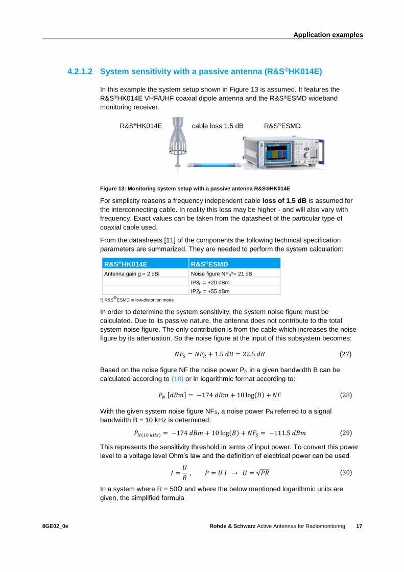
4.2.1.2 System sensitivity with a passive antenna (R&S®HK014E)

In this example the system setup shown in Figure 13 is assumed. It features the

R&S®HK014E VHF/UHF coaxial dipole antenna and the R&S®ESMD wideband

monitoring receiver.

Figure 13: Monitoring system setup with a passive antenna R&S®HK014E

For simplicity reasons a frequency independent cable loss of 1.5 dB is assumed for

the interconnecting cable. In reality this loss may be higher - and will also vary with

frequency. Exact values can be taken from the datasheet of the particular type of

coaxial cable used.

From the datasheets [11] of the components the following technical specification

parameters are summarized. They are needed to perform the system calculation:

R&S®HK014E R&S®ESMD

Antenna gain g = 2 dBi Noise figure NFR*= 21 dB

IP3R = +20 dBm

IP2R = +55 dBm

*) R&S®

ESMD in low-distortion mode

In order to determine the system sensitivity, the system noise figure must be

calculated. Due to its passive nature, the antenna does not contribute to the total

system noise figure. The only contribution is from the cable which increases the noise

figure by its attenuation. So the noise figure at the input of this subsystem becomes:

𝑁𝐹𝑆 = 𝑁𝐹𝑅 + 1.5 𝑑𝐵 = 22.5 𝑑𝐵 (27)

Based on the noise figure NF the noise power PN in a given bandwidth B can be

calculated according to (18) or in logarithmic format according to:

𝑃𝑁 [𝑑𝐵𝑚] = −174 𝑑𝐵𝑚 + 10 log(𝐵) + 𝑁𝐹 (28)

With the given system noise figure NFS, a noise power PN referred to a signal

bandwidth B = 10 kHz is determined:

𝑃𝑁(10 𝑘𝐻𝑧) = −174 𝑑𝐵𝑚 + 10 log(𝐵) + 𝑁𝐹𝑆 = −111.5 𝑑𝐵𝑚 (29)

This represents the sensitivity threshold in terms of input power. To convert this power

level to a voltage level Ohm’s law and the definition of electrical power can be used

𝐼 =𝑈

𝑅 , 𝑃 = 𝑈 𝐼 → 𝑈 = √𝑃𝑅 (30)

In a system where R = 50Ω and where the below mentioned logarithmic units are

given, the simplified formula

R&S®HK014E cable loss 1.5 dB R&S®ESMD



18

𝑈 [𝑑𝐵µ𝑉] = 𝑃50𝛺 [𝑑𝐵𝑚] + 107 𝑑𝐵 (31)

can be used yielding in a minimum detectable voltage level of

𝑈min (10 𝑘𝐻𝑧) = −4.5 𝑑𝐵µ𝑉 (32)

As explained in [1] the transformation from voltage to field strength is done via the

antenna factor k. If k is not specified for an antenna (which is the case for

R&S®HK014E) it can be derived from the gain value g with the formula:

𝑘[𝑑𝐵/𝑚] = −29.8 + 20 log (𝑓

𝑀𝐻𝑧) − 𝑔 [𝑑𝑏] (33)

At the relevant monitoring frequency fm= 200 MHz a gain of g = 2 dBi is specified in the

antenna datasheet, resulting in an antenna factor of

𝑘(200𝑀𝐻𝑧) = 14.2 𝑑𝐵/𝑚 (34)

As stated in (1) the antenna factor relates field strength to the measured voltage. If

logarithmic values are used, the minimum detectable field strength can now be

calculated by adding the antenna factor k to the minimum detectable voltage Umin

𝐸min(10 𝑘𝐻𝑧) = 𝑈min(10 𝑘𝐻𝑧) + 𝑘 ≈ 10 𝑑𝐵µ𝑉/𝑚 (35)

The mobile station as calculated in (26) generates a field strength of 15 dBµV/m.

Consequently the signal to noise ratio of the signal from the mobile station is only

𝑆𝑁𝑅𝑚𝑜𝑏𝑖𝑙𝑒 = 15 𝑑𝐵µ𝑉/𝑚 − 10 𝑑𝐵µ𝑉/𝑚 = 𝟓 𝒅𝑩 (36)

which is a very low value that can be regarded "at the edge" of intelligibility of an FM

modulated signal in a 10 kHz bandwidth.

4.2.1.3 System sensitivity with an active antenna (R&S®HE600)

It is assumed that the system setup as shown in Figure 14 is used at the monitoring

location.

Figure 14: Monitoring system setup with an active antenna and bias unit

R&S®HE600 R&S®ESMD

R&S®IN600



19

This setup comprises of the R&S®HE600 active omnidirectional receiving antenna, the

R&S®IN600 bias unit and the R&S®ESMD wideband monitoring receiver.

From the datasheets of the components [9, 10] the following specification values

required for the system calculation can be derived:

R&S®HE600 R&S®IN600 R&S®ESMD

Practical gain gp= 12 dB (@ 200 MHz) Insertion loss l = 1.5 dB Noise figure NF = 21 dB

Sensitivity Emin= -41 dBµV/m (@ 200 MHz, measured in a 1Hz bandwidth)

IP3R = +20 dBm

IP3A = +28 dBm IP2R = +55 dBm

IP2A = +50 dBm

For simplicity the loss of the cables interconnecting the three devices is neglected in

this example.

In the first step the overall system sensitivity is determined. Due to the fact that various

components add noise to the system, the specification of the antenna alone is not

sufficient and the overall system sensitivity must be calculated.

For the active antenna, the field strength sensitivity is already provided in its datasheet.

In order to perform a system calculation that sensitivity must be converted into a noise

figure.

Using formula (8) in 3.4 and solving it for the antenna noise figure results in:

𝑁𝐹𝑎 = 𝐸𝑚𝑖𝑛 + 96.8 𝑑𝐵µ𝑉/𝑚 − 20 log (𝑓

𝑀𝐻𝑧) − 10 log (

𝐵

𝐻𝑧) +

𝐷

𝑑𝐵 (37)

For the directivity, D = 2.15 dB is assumed because the antenna can be approximated

as a half-wave dipole at 200 MHz. B is the bandwidth for which the sensitivity is

specified, so B = 1 Hz, consequently the noise figure results in:

𝑁𝐹𝑎 = 11.9 𝑑𝐵 (38)

For further calculations it is also required to know the electronic gain GT which can be

determined from the practical gain by solving formula (13) for GT

𝐺𝑇 = 𝐺𝑃

𝐷 (39)

or - when the values are given in logarithmic units - by simply subtracting the directivity

from the practical gain resulting in:

𝑔𝑇 = 12 𝑑𝐵 − 2.15 𝑑𝐵 = 9.85 𝑑𝐵 (40)

With these values it is now possible to calculate the total system noise figure FS based

on (9). Prior to this, the insertion loss l of the bias unit is added to the noise figure of

the receiver resulting in a combined noise figure

𝑁𝐹𝑅 = 21 𝑑𝐵 + 1.5 𝑑𝐵 = 22.5 𝑑𝐵 (41)



20

This simplification can be done due to the passive nature of the bias unit (in terms of

the RF path). The overall system noise figure FS can then be calculated:

𝐹𝑆 = 𝐹𝑎 + 𝐹𝑅 − 1

𝐺𝑇

≈ 33.8 → 𝑁𝐹𝑆 ≈ 15 𝑑𝐵 (42)

Based on the system noise figure NFS the minimum detectable field strength in a

bandwidth B =10 kHz can now be calculated using formula (8) in 3.4:

𝐸𝑚𝑖𝑛(10 𝑘𝐻𝑧) = −96.8 𝑑𝐵µ𝑉/𝑚 + 46 𝑑𝐵 + 40 𝑑𝐵 + 15 𝑑𝐵 − 2.15 𝑑𝐵 ≈ 𝟐 𝒅𝑩µ𝑽/𝒎 (43)

As already calculated in 4.2.1.1, the mobile station will generate a field strength of

Emobile= 15 dBµV/m. Thus the achievable signal-to-noise ratio of a setup comprising of

the R&S®HE600 active omnidirectional receiving antenna can be calculated:

𝑆𝑁𝑅𝑚𝑜𝑏𝑖𝑙𝑒 = 15 𝑑𝐵µ𝑉/𝑚 − 2 𝑑𝐵µ𝑉/𝑚 = 𝟏𝟑 𝒅𝑩 (44)

This results in a significant improvement of signal intelligibility compared to the solution

with a passive antenna described in 4.2.1.2.

Not to forget the reduced space requirements of the active antenna solution, and the

fact that the monitoring system is capable of covering a much larger bandwidth

compared to the passive antenna approach.

4.2.2 Scenario 2 - Reception of a weak signal in the presence of strong

interference

Now additionally to scenario 1 described in 4.2.1 an FM broadcast station is located at

a distance of 3 km from the monitoring location - so in close vicinity (see Figure 15)

The FM Broadcast station transmits two radio programs on different frequencies with

the following parameters

Mobile station Monitoring

location

FM Broadcast station

30 km 3 km

Figure 15: Example scenario for monitoring of a weak signal in the presence of strong interference



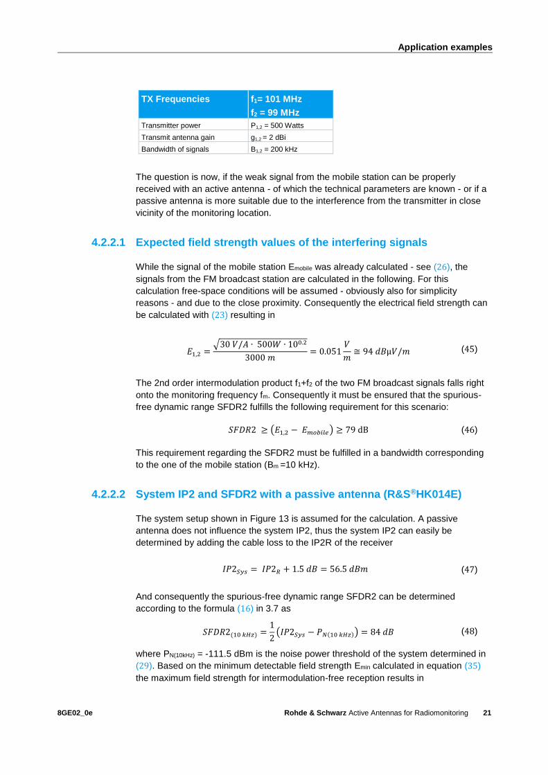
21

TX Frequencies f1= 101 MHz

f2 = 99 MHz

Transmitter power P1,2 = 500 Watts

Transmit antenna gain g1,2 = 2 dBi

Bandwidth of signals B1,2 = 200 kHz

The question is now, if the weak signal from the mobile station can be properly

received with an active antenna - of which the technical parameters are known - or if a

passive antenna is more suitable due to the interference from the transmitter in close

vicinity of the monitoring location.

4.2.2.1 Expected field strength values of the interfering signals

While the signal of the mobile station Emobile was already calculated - see (26), the

signals from the FM broadcast station are calculated in the following. For this

calculation free-space conditions will be assumed - obviously also for simplicity

reasons - and due to the close proximity. Consequently the electrical field strength can

be calculated with (23) resulting in

𝐸1,2 =√30 𝑉/𝐴 ∙ 500𝑊 ∙ 100.2

3000 𝑚= 0.051

𝑉

𝑚≅ 94 𝑑𝐵µ𝑉/𝑚 (45)

The 2nd order intermodulation product f1+f2 of the two FM broadcast signals falls right

onto the monitoring frequency fm. Consequently it must be ensured that the spurious-

free dynamic range SFDR2 fulfills the following requirement for this scenario:

𝑆𝐹𝐷𝑅2 ≥ (𝐸1,2 − 𝐸𝑚𝑜𝑏𝑖𝑙𝑒) ≥ 79 dB (46)

This requirement regarding the SFDR2 must be fulfilled in a bandwidth corresponding

to the one of the mobile station (Bm =10 kHz).

4.2.2.2 System IP2 and SFDR2 with a passive antenna (R&S®HK014E)

The system setup shown in Figure 13 is assumed for the calculation. A passive

antenna does not influence the system IP2, thus the system IP2 can easily be

determined by adding the cable loss to the IP2R of the receiver

𝐼𝑃2𝑆𝑦𝑠 = 𝐼𝑃2𝑅 + 1.5 𝑑𝐵 = 56.5 𝑑𝐵𝑚 (47)

And consequently the spurious-free dynamic range SFDR2 can be determined

according to the formula (16) in 3.7 as

𝑆𝐹𝐷𝑅2(10 𝑘𝐻𝑧) =1

2(𝐼𝑃2𝑆𝑦𝑠 − 𝑃𝑁(10 𝑘𝐻𝑧)) = 84 𝑑𝐵 (48)

where PN(10kHz) = -111.5 dBm is the noise power threshold of the system determined in

(29). Based on the minimum detectable field strength Emin calculated in equation (35)

the maximum field strength for intermodulation-free reception results in



22

𝐸max(10 𝑘𝐻𝑧) = 𝐸min(10 𝑘𝐻𝑧) + 𝑆𝐹𝐷𝑅2(10 𝑘𝐻𝑧) = 10 𝑑𝐵µ𝑉/𝑚 + 84 dB = 94 𝑑𝐵µ𝑉/𝑚 (49)

This corresponds exactly to the field strength caused by the FM broadcast station as

determined in equation (45).

4.2.2.3 Conclusion for the passive antenna approach

Figure 16: Levels of field strength for a system with a passive antenna

With the passive antenna system setup, the signal to noise ratio of the mobile station is

marginal at only 5 dB. The SFDR2 is 5 dB higher than the requirement determined in

4.2.2.1. Figure 16 shows the different signal levels. So in order to be able to detect a

signal with a certain margin, the actual SFDR2 always has to be exactly this margin

higher than the SFDR2 requirement. Essentially a higher dynamic range is bought with

less sensitivity. In the particular example the receiving system is ideally matched to the

field strength levels caused by the interfering signal.

It was already mentioned that the achieved S/N of 5 dB is relatively low - and it may

not be sufficient for the reception of certain signals. Note that the required S/N levels

will depend on the type of modulation as well as on the bandwidth of the signal.

An improvement of the system sensitivity can either be achieved by using an active

antenna as described in 4.2.1.3, or by using a directional antenna, for example the

R&S®HL033 log-periodic broadband antenna [14]. Such an antenna will significantly

improve the situation, when the interfering signal is arriving from a different direction

than the wanted signal. On the one hand it will increase the signal of the mobile station

due to its higher passive gain of approx. g = 6.5 dBi compared to gomni = 2 dBi of an

omnidirectional antenna like R&S®HK014E. On the other hand it will also reduce the

signal levels of the interfering signals - simply due to its radiation pattern (see Figure

17) and the corresponding attenuation for signals arriving from directions outside the

antenna's main lobe.



23

Figure 17: R&S HL033 log-periodic broadband antenna and its E-field pattern at 200 MHz

Consequently, the minimum detectable field strength can be improved to a value of

Emin = 5.5 dBµV/m (in a 10 kHz bandwidth) - resulting in an S/N ratio of 9.5 dB - while

the SFDR2 can reach values >100 dB, when the interferer is located in the opposite

direction (assuming an antenna front-to back ratio of typ. 25 dB).

However it must not be neglected that a directional antenna always needs to be

aligned to the target. This can be achieved by means of an antenna rotator - but limits

the usability as simultaneous reception of signals arriving from substantially different

directions is not possible any more.

4.2.2.4 System IP2 and SFDR2 with an active antenna (R&S®HE600)

When the setup with the R&S®HE600 active omnidirectional receiving antenna as

shown in Figure 14 is used, the system IP2 can be calculated with formula (15). It is

worth mentioning that the data for the antenna intercept points listed in the datasheet

are already referring to the output of the antenna. Consequently the gain of the

antenna must not be part of the initial calculation of the system 2nd order intercept

point. The only additional parameter for the calculation of the cascaded intercept point

is the loss of the cable (or here the insertion loss of the bias unit).

After using the linear values in formula (15) the system 2nd order intercept point

becomes:

OIP2Sys =1

(√1

105.5 + √1

105 ∙ 10−0.15)

2 ≈ 32621 mW ≅ 45.1 dBm (50)

As indicated by the letter "O" this value is referring to the output of the system, hence

to the receiver output.

But for the calculation of the spurious-free dynamic range (SFDR2) the input intercept

point of the system is required. It can be determined by subtracting the so called

system gain GSys from the output intercept point.



24

𝐼𝐼𝑃2𝑆𝑦𝑠 = 𝑂𝐼𝑃2𝑆𝑦𝑠 − 𝐺𝑠𝑦𝑠 [𝑑𝐵] (51)

The system gain is defined as the overall gain in the chain between the passive

radiator and the output of the receiver. In this case it can be calculated as

𝐺𝑆𝑦𝑠 = 𝐺𝑇 + 𝐺𝑐𝑎𝑏𝑙𝑒 = 9.85 𝑑𝐵 − 1.5 𝑑𝐵 = 8.35 𝑑𝐵 (52)

Consequently the following input intercept point can be determined

𝐼𝐼𝑃2𝑆𝑦𝑠 = 45.1 𝑑𝐵𝑚 − 8.35 𝑑𝐵𝑚 ≈ 36.8 𝑑𝐵𝑚 (53)

Before the SFDR2 can be calculated by means of formula (16), the noise power PN in

the corresponding bandwidth B = 10 kHz must be known which is based on the system

noise figure NFS determined in (42).

According to formula (28) this results in the following value

𝑃𝑁(10𝑘𝐻𝑧) = −174 𝑑𝐵𝑚 + 𝑁𝐹𝑠 + 10 log(𝐵) = −174 + 15 + 40 = −119 𝑑𝐵𝑚 (54)

Finally the SFDR2 can be asserted:

𝑆𝐹𝐷𝑅2(10 𝑘𝐻𝑧) = 1

2(−36.8 𝑑𝐵𝑚 − (−119 𝑑𝐵𝑚)) ≈ 78 𝑑𝐵 (55)

Based on the minimum detectable field strength previously determined (see (43)), the

maximum field strength for intermodulation-free operation is calculated:

𝐸max(10 𝑘𝐻𝑧) = 𝐸min(10 𝑘𝐻𝑧) + 𝑆𝐹𝐷𝑅2(10 𝑘𝐻𝑧) = 2 𝑑𝐵µ𝑉/𝑚 + 78𝑑𝐵 = 80𝑑𝐵µ𝑉/𝑚 (56)

4.2.2.5 Conclusion for the active antenna approach

As already shown in chapter 4.2.1.3, the signal from the mobile station can be detected

with 13 dB above the minimum detectable field strength of the system. Hence without

the interference from the FM broadcast station a significant improvement compared to

the passive antenna approach can be achieved

Although the SFDR2 requirement of 79 dB determined in 4.2.2.1 is nearly met, the

absolute field strength of the two FM signals is 14 dB higher than the maximum

allowed field strength for intermodulation-free reception (Emax).

As a consequence a strong 2nd order intermodulation product is generated at

fm = f1+f2 = 200 MHz as shown in orange color in Figure 18.



25

Figure 18: Levels of signals and intermodulation products for an active antenna approach

Because 2nd order intermodulation products rise with 2 dB for every 1 dB of increased

input level, the IM2 product will be 28 dB above the noise floor and thus completely

mask the signal from the mobile station making reception impossible.

Consequently the fulfilment of the spurious-free dynamic range requirement alone

does not yet ensure that intermodulation products are not generated. The far more

important parameter here is the maximum field strength for intermodulation-free

reception Emax.

So the dynamic range parameters always have to be seen in the context of the

absolute values for field strength.

4.2.3 Other measures to reduce or avoid intermodulation

In an application scenario where the interfering signals are higher than the maximum

field strength for intermodulation-free reception, it is possible to add an attenuator

between the passive antenna and the receiver. Obviously such an attenuator will also

decrease the sensitivity and hence the min. detectable field strength is reduced.

A better approach is the usage of band-stop filters tuned to the interfering signal's

frequency. Obviously this is only possible when there is a significant offset between the

receiving frequency and the interfering signal frequency. While this usually works for

2nd order Intermodulation, for 3rd order intermodulation products the approach is

hardly feasible as the intermodulation products are very close to the interferer's

frequencies.

Note that for the system with the active antenna as described in Figure 14 none of the

before mentioned measures can easily be implemented. This is due to the fact that the

interface between the passive radiators and the active circuitry is not accessible for

any filtering or attenuation measures. Consequently in a system with an active antenna



26

the intermodulation performance of the antenna is dominating the overall system

performance.

Active antenna circuit design has to be projected carefully in order to avoid poor

robustness to intermodulation. A common practice is to use push-pull amplifiers made

of complementary transistors. Other design options are the usage of a current

feedback loop or including a switching circuit to bypass the active element (which

obviously increases mismatch and consequently decreases the overall system

sensitivity). However it must be mentioned that improvement of the active antenna's

IP2 or IP3 values beyond the receiver values will not cause noticeable improvements

of the overall system intermodulation performance.

4.3 HF example scenario

In the previous examples describing the reception of VHF signals it was assumed that

the polarizations of both antennas match - meaning that the signal is transmitted and

received by (in this case) a vertically polarized antenna. For the simplified assumption

of free space conditions this is valid. In reality however the signal may undergo certain

changes regarding its polarization caused by reflections from obstacles on the

propagation path.

4.3.1 Effects on polarization caused by the ionosphere

At HF frequencies the situation is different - especially if ground-wave propagation is

neglected and the focus is on signals being reflected at the ionosphere - so called sky-

wave signals. Due to the largely anisotropic permittivity of the layers in the

ionosphere, the signal which is transmitted through or reflected by its different layers

will always be subject to polarization changes. This means for certain frequencies at

certain elevation angles the polarization may be turned from horizontal to vertical, while

at other frequencies the wave may become circularly or even elliptically polarized.

It is therefore of large benefit to have an antenna where the polarization can be

switched, or alternatively to have several antennas with different fixed polarizations, so

that the best one for a certain signal can be selected.

4.3.2 Field strength measurement at HF using different types of

antennas

Compared to VHF or UHF the determination of precise field strength values at HF

frequencies is rather difficult to achieve. This is due to the particular propagation of

waves in this frequency range and due to the fact that the parameters of an HF

antenna are not only determined by the antenna itself but also by the properties of its

surroundings. This applies to passive antennas as well as to active antennas, although

active antennas are generally less sensitive to coupling effects with their surroundings.



27

4.3.2.1 Vertically polarized monopoles

However for monopole antennas like the R&S®HE010E active rod antenna this effect

can immediately be seen by looking at the antenna's vertical radiation pattern taken

from the datasheet [13] as shown in Figure 19.

Figure 19: R&S®HE010E Vertical radiation pattern

While the two curves labeled with 10 kHz and 80 MHz are valid for an installation

above a perfectly conducting and infinitely large plane, the curve labeled with

moderately conducting plane shows a significant reduction of field strength for signals

arriving at angles close to the horizon (here ϑ = 90°). Further reductions would occur

above a poorly conducting plane and even further loss when the dimensions of the

ground plane would be reduced to values below the order of approx. half a wavelength.

Antenna gain (and consequently also the antenna factor) is defined at the maximum of

radiation, which in the case of a moderately conducting plane occurs at ϑ ≈ 70°, but

may strongly vary depending on the properties of the ground plane.

For sky-wave signals reflected by the ionosphere the situation is even more uncertain,

because the exact angle of arrival is unknown. Simulation tools can determine this

value based on a series of input parameters like distance to the transmitter, frequency,

time of day, time of year and the smoothed number of sunspots (SSN). However they

cannot omit that for closer distances the so called near vertical incident sky-waves

(NVIS) reflected by the F2 layer in the ionosphere fall right into a null of the monopole's

vertical radiation pattern as described in [15].

0 200 0 200 400 600 800

1000 1200km

h

80°

Figure 20: Angle of incidence depending on distance from the transmitter



28

Consequently signals from short distances (< 500 km) will arrive at angles of less than

ϑ ≈ 40° as can be derived from Figure 20 assuming a reflection at the F2 layer at a

height of approx. 300 km above ground (see blue curve).

Applying the antenna factor to such signals - if they can be detected at all - will cause

incorrect field strength values. Generally a monopole antenna is not suitable for the

reception of NVIS signals due to its particular elevation pattern. It exhibits a so-called

skip zone. This skip zone is the area in-between the maximum distance where ground

wave propagation still works and the minimum distance of reception for sky-wave

signals arriving at angles of ϑ that are large enough in order not to fall into the null of

the antenna.

The reception in this skip zone is largely reduced and consequently an accurate field

strength calculation is not possible.

The expansion of the skip zone is not constant and will depend on all parameters that

affect HF wave propagation in general. The outer limit of 500 km as shown in Figure 21

is just an average value applicable for lower frequencies. For example, during daytime

in the summer season - when the height of the F2 layer is generally higher - the skip

zone can extend far beyond 1000 km for frequencies close to the MUF (maximum

usable frequency).

In summary vertically polarized monopole antennas are ideally suited for the reception

of ground waves as well as sky-waves of low angle of incidence above the horizon (ϑ

close to 90°). The latter type of signals usually originate at larger distances.

100 200 300 400 500 km

Skip zone

Area covered by ground waves

Area covered by sky waves

Figure 21: Skip zone of a vertically polarized monopole



29

4.3.2.2 NVIS antennas

For the reception of sky-wave signals from closer distances that arrive at higher angles

of incidence compared to the horizon (ϑ ≤ 40° as shown in Figure 20) a different type

of antenna is commonly used.

Such antennas are usually referred to as NVIS antennas. Looking at the vertical

radiation pattern of a horizontally polarized dipole , e.g. the R&S®HE010D active HF

dipole shown in Figure 22 reveals that the main lobe is pointing straight up to the sky

(ϑ=0°) for the lower and middle part of the HF frequency range.

Figure 22: Vertical radiation pattern of the R&S®HE010D active HF dipole installed on a 6 m mast

Only at the upper end of the HF frequency spectrum (30 MHz) the vertical pattern

starts to deteriorate and shows nulls in-between its major lobes. However as these

patterns are based on an installation above a perfectly conducting plane, in a real

situation (i.e. above a moderately conducting plane) the nulls will be "filled up" - and

thus the antenna becomes usable for NVIS signals in the entire HF frequency range.

4.3.3 Selecting an appropriate HF antenna

As just explained, different types of HF antennas may be needed depending on the

type of signal (and its corresponding angle of incidence). The R&S®HE016 active

antenna system shown in Figure 23 overcomes the need for multiple antennas

because it contains a vertically polarized monopole antenna and two horizontally

polarized dipoles that are oriented perpendicular to each other. All antennas are of an

active type with shortened radiators so that the dimensions of the system (approx. 3 x

3 x 1.5 m) can be kept relatively small.



30

Figure 23: R&S®HE016 active antenna system

The outputs of the two horizontally polarized dipoles are combined via a 90° coupler to

form a so called turnstile antenna. This allows reception of horizontally polarized

signals with an almost omnidirectional radiation pattern when they arrive at angles of

incidence close to the horizon (ϑ approaching 90°). For high angle of incidence signals

(ϑ approaching 0°) the combination of both dipoles via the coupler results in a circularly

polarized antenna, which is generally suitable to receive signals of any polarization

with bearable loss.

For vertically polarized signals arriving at angles of incidence close to the horizon (e.g.

ground wave signals) the vertical monopole is used - its output is available at a 2nd RF

connector which allows switching between the two signal paths. This makes

R&S®HE016 an ideal solution for almost any kind of signals present in the HF

frequency range. However there are certain effects that must be taken into account

when it is installed on a mast.

4.3.3.1 Effects of installation height

For the vertical section (monopole) of R&S®HE016 the open circuit voltage UOC of the

passive radiator depends on the height of the mast. This will lead to a directly

proportional increase of the sensitivity up to mast height of approx. 0.15 λ.

Beyond this height, mast resonances will occur at the following approximate heights:

ı at resonance point ℎ = 𝑛 ∙𝜆

4(𝑤𝑖𝑡ℎ 𝑛 = 1,3,5, … ),

with voltage peaks causing a high risk of non-linear distortions

ı at resonance point ℎ = 𝑛 ∙𝜆

4(𝑤𝑖𝑡ℎ 𝑛 = 2,4,6, ),

with voltage dips resulting in a high risk of reduced sensitivity

On the other hand a certain height of the mast has to be maintained for the horizontally

polarized dipoles of the antenna system because here close proximity to the ground

will result in increased loss due to coupling effects. So a reasonable compromise for

vertical and horizontal polarization is obtained at mast heights between 4 m and 7 m.



31

Figure 24 illustrates the mast resonances by comparing the practical gain at different

heights of the supporting mast. Note that the values for the horizontally polarized part

are shown for installation on a 6 m mast only.

Figure 24: R&S®HE016 practical gain with mast resonances

Obviously the gain variation also influences the antenna factor. The assumption of an

almost constant antenna factor for the vertical part of the antenna system - which is

essentially a monopole as described in 3.2 - is no longer valid when R&S®HE016 is

installed on a mast. This has to be taken into account when field strength values are to

be determined at HF frequencies. Figure 25 shows this effect very clearly.

Figure 25: R&S®HE016 antenna factor depending on mast height

It must be noted that the problem of mast resonances persists if a mast made of non-

conducting material is used and the coaxial cable is routed vertically without any

decoupling (such as ferrite rings etc.) applied to it. The cable then acts almost like a

mast. So in order to reduce the resonances, proper decoupling measures of the

vertically run coaxial cable have to be taken.



32

4.3.4 Active HF monitoring antennas summarized

The selection of HF monitoring antennas has to be mainly based on the distance to the

transmitter that they are supposed to detect. Also their installation height must be

chosen carefully as it will affect many parameters that may lead to poor reception or

coverage of the wanted signals. Not to forget the influence of external noise (either

man-made or atmospheric) and the effects of intermodulation from close-by

transmitters which have been dealt with in chapters 3 extensively, hence they are not

mentioned in detail here again.

Monitoring antennas are dedicated to receive signals with the best possible S/N. It is

not their aim to measure exact values of field strength. This is especially true for active

HF monitoring antennas where the parameters of the antenna depend on various

external factors. Consequently a calibration of active HF monitoring antennas

hardly makes sense and is usually not offered by Rohde & Schwarz.

The typical values for gain, antenna factor or radiation pattern specified for defined

surroundings are usually sufficient for most applications of this type of antennas.

Literature


33

5 Literature

[1] Reckeweg/Rohner: Antenna Basics White Paper (R&S Application Note 8GE01)

[2] Bianchi/Meloni: Natural and man-made terrestrial electromagnetic noise: an

outlook (Annals of geophysics Vol. 50, N. 3rd June 2007)

[3] Sainati/Fessenden: Performance of an electrically small antenna amplifier circuit

(IEEE Transactions on aerospace and electronic systems, Vol. AES-17 No.1, Jan

1981)

[4] Low-Noise JFETs - Superior Performance to Bipolars, (Siliconix Application Note

AN106, March 1997)

[5] Minihold/Wagner: Measuring the Nonlinearities of RF-Amplifiers using Signal

Generators (Rohde & Schwarz Application Note 1MA71)

[6] Demmel: Kenngrößen aktiver Antennen, (nachrichten elektronik 34(1980) Heft 9)

[7] Rohde/Whitaker: Communications Receivers, 3rd edition 2000, McGraw Hill

[8] Calculating Radiated power and Field Strength for Conducted Power

Measurements, Semtech technical note TN1200.04, www.semtech.com

[9] R&S®HE600 Active Omnirectional Receiving Antenna - brief description

(http://cdn.rohde-schwarz.com/pws/dl_downloads/dl_common_library/

dl_brochures_and_datasheets/pdf_1/HE600_cat_2015_72-73.pdf)

[10] R&S®IN600 Bias Unit - brief description


dl_brochures_and_datasheets/pdf_1/IN600_cat_2015_160-161.pdf)

[11] R&S®HK014E VHF/UHF Coaxial Dipole- brief description


dl_brochures_and_datasheets/pdf_1/HK014E_cat_2015_100-101.pdf)

[12] R&S®HE016 Active Antenna System - brief description


dl_brochures_and_datasheets/pdf_1/HE016_cat_2015_26-27.pdf)

[13] R&S®HE010E Active Rod Antenna - brief description


dl_brochures_and_datasheets/pdf_1/HE010E_cat_2015_24-25.pdf)

[14] R&S®HL033 Log-Periodic Broadband Antenna - brief description


dl_brochures_and_datasheets/pdf_1/HL033_cat_2015_78-79.pdf)

[15] Stark: Propagation of electromagnetic waves (Neues von Rohde & Schwarz

Nr.112 to 115, 1986

Glossary


34

6 Glossary

DR1 Linear dynamic range (1dB compression)

FET Field effect transistor

FM Frequency modulation

HF High frequency (3 MHz to 30 MHz)

IP2 Second order intercept point (usually referred to the input unless noted)

IP3 Third order intercept point (usually referred to the input unless noted)

JFET Junction field effect transistor

LF Low frequency (30 kHz to 300 kHz)

MF Medium frequency (300 kHz to 3 MHz)

MUF Maximum usable frequency

NF Noise figure

NVIS Near vertical incidence sky-wave

OIP2 Output second order intercept point

OIP3 Output third order intercept point

SFDR Spurious-free dynamic range

SHF Super high frequency (3 GHz to 30 GHz)

S/N or SNR Signal to noise ratio

SSN Smoothed sunspot number

UHF Ultra high frequency (300 MHz to 3 GHz)

VHF Very high frequency (30 MHz to 300 MHz)


35

Rohde & Schwarz

The Rohde & Schwarz electronics group offers

innovative solutions in the following business fields:

test and measurement, broadcast and media, secure

communications, cybersecurity, radiomonitoring and

radiolocation. Founded more than 80 years ago, this

independent company has an extensive sales and

service network and is present in more than 70

countries.

The electronics group is among the world market

leaders in its established business fields. The

company is headquartered in Munich, Germany. It

also has regional headquarters in Singapore and

Columbia, Maryland, USA, to manage its operations

in these regions.

Regional contact

Europe, Africa, Middle East +49 89 4129 12345 [email protected] North America 1 888 TEST RSA (1 888 837 87 72) [email protected] Latin America +1 410 910 79 88 [email protected] Asia Pacific +65 65 13 04 88 [email protected]

China +86 800 810 82 28 |+86 400 650 58 96 [email protected]

Sustainable product design

ı Environmental compatibility and eco-footprint

ı Energy efficiency and low emissions

ı Longevity and optimized total cost of ownership

This and the supplied programs may only be used

subject to the conditions of use set forth in the

download area of the Rohde & Schwarz website.

R&S® is a registered trademark of Rohde & Schwarz GmbH & Co.

KG; Trade names are trademarks of the owners.

Rohde & Schwarz GmbH & Co. KG

Mühldorfstraße 15 | 81671 Munich, Germany

Phone + 49 89 4129 - 0 | Fax + 49 89 4129 – 13777

www.rohde-schwarz.com

PA

D-T

-M: 3573.7

380.0

2/0

2.0

5/E

N/

mailto:[email protected]





Date post:	22-Mar-2018
Category:	Documents
Upload:	buiduong
View:	225 times
Download:	2 times

Appl. Note, Active Antennas for Radiomonitoring · PDF fileActive Antennas for Radiomonitoring...

Documents