179
Application and Verification of ECMWF products in Member States and Co-operating States Report 2006 August 2006

Application and Verification of ECMWF products in
Member States and Co-operating States
Report 2006
August 2006

ContentsPart I: Summary
Introduction. . . . . . . . . . . . . . . . . . . . . . . . . . . . . . . . . . . . . . . . . . . . . . . . . . . . . . . . . . . . . . . . . . i
Annex . . . . . . . . . . . . . . . . . . . . . . . . . . . . . . . . . . . . . . . . . . . . . . . . . . . . . . . . . . . . . . . . . . . . A1
Part II: Reports from Member States and Co-operating States
Austria. . . . . . . . . . . . . . . . . . . . . . . . . . . . . . . . . . . . . . . . . . . . . . . . . . . . . . . . . . . . . . . . . . . . . 1
Belgium . . . . . . . . . . . . . . . . . . . . . . . . . . . . . . . . . . . . . . . . . . . . . . . . . . . . . . . . . . . . . . . . . . . . 8
Croatia . . . . . . . . . . . . . . . . . . . . . . . . . . . . . . . . . . . . . . . . . . . . . . . . . . . . . . . . . . . . . . . . . . . 14
Czech Republic . . . . . . . . . . . . . . . . . . . . . . . . . . . . . . . . . . . . . . . . . . . . . . . . . . . . . . . . . . . . . . 20
Denmark . . . . . . . . . . . . . . . . . . . . . . . . . . . . . . . . . . . . . . . . . . . . . . . . . . . . . . . . . . . . . . . . . . 21
Finland . . . . . . . . . . . . . . . . . . . . . . . . . . . . . . . . . . . . . . . . . . . . . . . . . . . . . . . . . . . . . . . . . . . 23
France . . . . . . . . . . . . . . . . . . . . . . . . . . . . . . . . . . . . . . . . . . . . . . . . . . . . . . . . . . . . . . . . . . . . 28
Germany . . . . . . . . . . . . . . . . . . . . . . . . . . . . . . . . . . . . . . . . . . . . . . . . . . . . . . . . . . . . . . . . . . 33
Greece . . . . . . . . . . . . . . . . . . . . . . . . . . . . . . . . . . . . . . . . . . . . . . . . . . . . . . . . . . . . . . . . . . . . 39
Hungary . . . . . . . . . . . . . . . . . . . . . . . . . . . . . . . . . . . . . . . . . . . . . . . . . . . . . . . . . . . . . . . . . . 44
Iceland. . . . . . . . . . . . . . . . . . . . . . . . . . . . . . . . . . . . . . . . . . . . . . . . . . . . . . . . . . . . . . . . . . . . 55
Ireland . . . . . . . . . . . . . . . . . . . . . . . . . . . . . . . . . . . . . . . . . . . . . . . . . . . . . . . . . . . . . . . . . . . . 62
Italy . . . . . . . . . . . . . . . . . . . . . . . . . . . . . . . . . . . . . . . . . . . . . . . . . . . . . . . . . . . . . . . . . . . . . . 74
Netherlands . . . . . . . . . . . . . . . . . . . . . . . . . . . . . . . . . . . . . . . . . . . . . . . . . . . . . . . . . . . . . . . . 85
Norway . . . . . . . . . . . . . . . . . . . . . . . . . . . . . . . . . . . . . . . . . . . . . . . . . . . . . . . . . . . . . . . . . . . 90
Portugal. . . . . . . . . . . . . . . . . . . . . . . . . . . . . . . . . . . . . . . . . . . . . . . . . . . . . . . . . . . . . . . . . . . 99
Romania . . . . . . . . . . . . . . . . . . . . . . . . . . . . . . . . . . . . . . . . . . . . . . . . . . . . . . . . . . . . . . . . . 107
Serbia. . . . . . . . . . . . . . . . . . . . . . . . . . . . . . . . . . . . . . . . . . . . . . . . . . . . . . . . . . . . . . . . . . . . 117
Slovenia. . . . . . . . . . . . . . . . . . . . . . . . . . . . . . . . . . . . . . . . . . . . . . . . . . . . . . . . . . . . . . . . . . 123
Spain. . . . . . . . . . . . . . . . . . . . . . . . . . . . . . . . . . . . . . . . . . . . . . . . . . . . . . . . . . . . . . . . . . . . 127
Sweden . . . . . . . . . . . . . . . . . . . . . . . . . . . . . . . . . . . . . . . . . . . . . . . . . . . . . . . . . . . . . . . . . . 134
Switzerland . . . . . . . . . . . . . . . . . . . . . . . . . . . . . . . . . . . . . . . . . . . . . . . . . . . . . . . . . . . . . . . . 141
Turkey . . . . . . . . . . . . . . . . . . . . . . . . . . . . . . . . . . . . . . . . . . . . . . . . . . . . . . . . . . . . . . . . . . . 144
United Kingdom . . . . . . . . . . . . . . . . . . . . . . . . . . . . . . . . . . . . . . . . . . . . . . . . . . . . . . . . . . . . 153

Part 1
Summary

i
1. IntroductionIn May 2006 Member States and Co-operating States were requested to contribute to the Report on Application and Verificationof ECMWF Products for 2006. Contributions have been received from 24 States and constitute the second part of this report.The first part presents a summary of the information and results given in the contributions – these were requested to be discussedunder the following headings:
1. Summary of major highlights
2. Objective verification
3. Subjective verification
4. Seasonal and monthly forecast
5. References to relevant publications
The recommendations to Member States for verification of local weather forecasts are given in ECMWF TechnicalMemorandum No 430 by P. Nurmi, available via the ECMWF website:
http://www.ecmwf.int/publications/library/do/references/list/14
This summary focuses on comments that have been made about verification results, or on results themselves, when methods(e.g. subjective verification) differ from those used operationally at ECMWF. ECMWF objectively verifies a wide range ofdirect model output (DMO): upper air parameters verified against analyses and observations, weather elements verified againstobservations or 0-24h forecasts. Various statistics, such as area means, time averages, etc., are produced. The EPS verificationis included in this system. These results are considered in a separate document on Verification statistics and evaluations ofECMWF forecasts (Document ECMWF/TAC/36(06)5).
The contributions from Member States and Co-operating States contained in the second part of this report complement, insome detail, the presentations on applications and verification made at the ECMWF Product Users’ Meeting, 14-16 June 2006.Some of the findings from this meeting are included in the following summary. The programme for the Users’ Meeting, togetherwith the presentations and the conclusions from the final discussion, can be found on the ECMWF website at:
http://www.ecmwf.int/newsevents/meetings/forecast_products_user/Presentations2006/index.html
In this summary we also used information collected during the visits to Member States and Co-operating States betweenautumn 2005 and spring 2006.
2. General commentsThe contributions from Member States and Co-operating States in the second part of this report demonstrate a wide range ofapplications of ECMWF products together with an impressive variety of verification results. The overall impression is verypositive. ECMWF products are widely used in the medium range. In the short range ECMWF products are also used by manycountries, often together with other models, especially limited area models. The use of the EPS in developing early warningsfor severe weather events appears to be increasing. The monthly forecast system is also being used and found to be skilful byseveral countries.
ECMWF forecast products on the web are now widely available and used in the forecast offices. Users appreciate the easeof access and the range of products provided.
3. Applications and verification results
3.1 Applications
• As well as providing boundary conditions for several limited area systems, the ECMWF model is often used as areference system against which to compare the performance of the limited-area forecasts. EPS members also provideboundary conditions for some limited-area ensemble systems.
• ECMWF model fields are used to drive trajectory and dispersion models (Austria, Czech Republic, France, Hungary),hydrological models (Austria, Czech Republic, Finland, Serbia, Sweden), agricultural crop models (Croatia, Serbia)and as a backup for a short-range road ice model (Ireland).
3.2 Synoptic evaluation
• Belgium noted some inconsistency between successive forecasts (00, 12 UTC) in forecasting the evolution of cut-off lows.
• Romania noted occasional underestimation of blocking over Eastern Europe.
• The UK reported improved scores for 2005 from their subjective evaluation of ECMWF forecasts.
• The Netherlands reported that 2005 was the best year yet for their verification of ECMWF forecasts based on objectiveclassification of upper air fields.
• France reported that the verification of the EPS tubing central cluster was not as good for 2005 as for 2004.

ii
3.3 Weather parameters
• Hungary reported that a large area of low stratus persisting for several weeks was not well predicted by the ECMWFmodel; consequently forecast temperatures were too cold. Slovenia also noted this problem. Conversely, Sweden reportedtoo much low cloud forecast in very cold situations and also too much fog over cold seas.
• Underestimation of extreme cold temperatures was reported by Ireland, Serbia and Sweden.
• Underestimation of heavy precipitation and overestimation of light precipitation was mentioned by Hungary, Norwayand Romania. The difficulty of verifying precipitation forecasts was also mentioned (Hungary, Iceland).
• Ireland noted a long-term positive trend in precipitation forecasts. Croatia noted improved precipitation bias in 2005.Romania reported a clear improvement in precipitation forecasts, while Turkey stated that their operational precipitationforecasts had improved.
3.4 Post-processing• Almost all countries apply statistical procedures to post-process ECMWF products. Perfect prog, MOS and Kalman
Filter methods are all used. The procedures are used mainly for surface weather parameters (including temperature,precipitation and wind) and are particularly effective in correcting systematic differences (biases) between the modelgrid box mean values and station observations.
• Statistical post-processing is also applied to EPS forecasts. Finland reported that dressing the EPS improves probabilityforecasts for winds. France calibrates EPS distribution using rank histogram and Bayesian Model Averaging. Germanyalso noted the need to calibrate the EPS for extreme events.
3.5 Severe weather
• Belgium has introduced an EPS-based alert system for precipitation, maximum temperature and a heat index; probabilityinformation is given for 4 risk categories.
• The UK First-Guess Early Warning System, based on EPS input, was shown to have consistently useful skill to day 4,with only a slow drop off in performance beyond day 4.
• The Netherlands is developing an early warning system, based on the EPS, to alert forecasters to potential severe events.
• A preliminary study of issuing weather warnings in Finland showed ECMWF forecasts are used both at short-range(together with HIRLAM) and medium range.
• Germany reported that the EPS is used to assess the potential occurrence of extreme weather events.
• Following encouraging results in spring 2005 (heavy rainfall and severe flooding), Romania now uses the EPSoperationally and especially for extreme events. The EFI is found useful for highlighting severe situations. The CzechRepublic plans to use EPS precipitation probabilities for flood warnings next spring. Hungary reported results from acase study in which the EPS provides a good signal for heavy precipitation.
• Working together with the regional Water Boards, the Netherlands has developed an automated warning system forflood risk management. Critical precipitation amounts and probability thresholds were chosen based on a cost-lossanalysis for each Water Board. Warnings are automatically generated from 9-day EPS probability forecasts of area-average precipitation for each region
3.6 Tropical cyclones
• France reported ECMWF forecasts to be particularly useful for tropical cyclones and for the tropics in general. Strikeprobability maps are used for TCs. Other tropical products include wave model EPSgrams that are useful for potentialcoastal flood warnings.
• The UK reported a comparison of UK and ECMWF tropical cyclone forecasts. Met Office forecasts are better in theshort range (ECMWF has no manual initialisation), while ECMWF tracks are better beyond day 3. The two modelshave different characteristics – ECMWF is better at deepening cyclones, whereas the Met Office model does better inthe weakening phase.
3.7 Monthly and seasonal forecasts
• Use of the monthly forecasts was reported by France, Croatia, Czech Republic, Hungary, Iceland, Norway, Romania,Serbia, Slovenia, Sweden and UK. The monthly products from the ECMWF website are often used.
• The seasonal forecasts are used either directly or in combination with other (often statistical) predictions to provideseasonal outlooks in Croatia, Denmark, Hungary, Norway, Romania, Serbia, Slovenia, Switzerland and UK. Some ofthese are made available to the public. The ECMWF seasonal forecast is used to assess the confidence for theMétéoFrance seasonal forecast.
• Several countries are providing the monthly and seasonal forecasts internally (via their intranet) and are assessing thepotential for using these products (Austria, Iceland, Switzerland and Turkey).

ANNEX ANNEX
Recommendations on the verification of local weather forecasts
Pertti Nurmi, December 2003
1. Introduction - BackgroundThe ECMWF Technical Advisory Committee (TAC) noted at its 32nd session (2002) that the “Recommendations on theverification of local weather forecasts” annexed to the annual Report on Verification of ECMWF products in Member Statesand Co-operating States (hereafter referred to as MS), the so-called “Green Book”, had been drafted some ten years ago. TheTAC therefore requested that these recommendations be reviewed and revised in the light of current circumstances.
Recent progress in numerical weather prediction, as well as developments in forecast verification methods has been vigorous.The advent of probabilistic methods into operational numerical weather prediction has taken place during the last decade, andwith the introduction of the Ensemble Prediction Systems (EPS) dramatically widened the use and applicability of NWP outputin operational weather services within ECMWF MSs.
There are, and have been, various verification activities under the auspices of WMO like the newly founded Working Groupon Verification (WGV) ([web 1]) within the World Weather Research Program (WWRP), or the more established verificationgroup under the Working Group on Numerical Experimentation (WGNE) (Bougeault, 2003; [ref 1]). The emphasis of the latteris focused on verification techniques oriented toward model developers, while the role of the WGV is more directed to endusers of high impact weather forecasts.
There is a host of recent important international conferences and workshops, either solely dedicated to verification issues, e.g.
• Workshop on Making Verification More Meaningful (Boulder, 2002; [ref 2], [web 2])
• WWRP/WMO Workshop on the Verification of Quantitative Precipitation Forecasts (Prague, 2001; [web 3])
• EUMETNET/SRNWP Mesoscale Verification Workshop (De Bilt, 2001; [ref 3])
or, with a strong verification context, e.g.
• International Conference on Quantitative Precipitation Forecasting (Reading, 2002; [ref 4])
• The biennial European Conference(s) on Applications of Meteorology (ECAM)
Two important textbooks with wide coverage on forecast verification methodologies need be highlighted, the earlier by Wilks(1995; [ref 5]) and the very recent by Jolliffe and Stephenson (2003; [ref 6]). A historical survey on verification methodologywas compiled by Stanski et al. (1989; [ref 7]).
The Internet has dramatically established itself as the media and the means to communicate information. There are manywebsites with a wealth of verification content and their value is undeniable (e.g. [web 4, 5, 6]). However, one is easily lost inthe web space where various different notations and formulae flourish depicting same methods and measures.
The past few years have seen efforts in harmonizing international verification practices. Strict rules to slavishly follow pre-defined verification measures and scores has proven to be a difficult and an undesirable task. Nevertheless, it is stronglyadvisable to adopt a general, coherent framework in forecast verification and to utilize common state-of-the-art methods. Oneexample toward this objective was the WMO/CBS realized Standardised Verification System for Long-Range Forecasts ([web7]). For purely model-based large-scale numerical forecasts standardisation is, however, fairly straightforward compared toharmonizing the verification of various local weather forecast products, originating at operational national weather offices,where forecasting practices, parameters, lead times, forecast lengths, valid periods etc. are typically quite different.
Most of the above has taken place since the previous ECMWF “Green Book” verification recommendations were produced.A revision is therefore justified. It is the objective of these updated recommendations to take into account recent developmentsand guidelines in verification and also to cope with new model developments and forecast products originating thereof, withoutneglecting the common traditional methods.
The original reasoning and ideology behind the recommendations and the eventual “Green Book” contributions by the MSshave, however, not changes in the course of time. The previous reports and the existing “verification history” they containserve as a valuable reference for future reports. The reports are meant as a forum to provide, on the one hand, valuable exchangeinformation between the MSs to learn from each others’ experiences and, on the other hand, to produce valuable feedbackto the Centre on MS’s verification activities and results of localized model behaviour, and even to distinguish possible modelweaknesses. The latter function does not necessarily fall into the primary activities of the ECMWF itself where a more globalverification approach is applied.
Chapter 2 of the recommendations provides some general guidelines, followed by an overview of the properties of variousverification measures for continuous meteorological variables (Chapter 3), for binary and multi-category weather events(Chapter 4) and for probabilistic forecasts (Chapter 5). Forecast value and the end user decision making issues associated with
A1

ANNEX ANNEX
forecast verification is covered briefly in Chapter 6, followed by a short Chapter 7 on other related issues concerning MSsverification activities. Proposals for means and measures to be followed up in MSs’ annual contributions to the “Green Book”are highlighted and proposed at the end of each chapter.
The recommendations are outlined, having taken into account what has been reported by MSs in the “Green Books” of recentyears, and, when appropriate, to be in harmony with the latest textbook on verification ([ref 6]), where an interested reader isreferred to. It is the idea to keep the proposal at a fairly simple level to enable and encourage easy and straightforwardapplicability. In addition, MSs are warmly welcome to contribute whatever local verification studies they may think of beingof general interest. At the end of the document, there are two lists of references, one to printed literature (quoted by [ref #] inthe text) and, the other, for recommended websites existing at the time of writing (quoted by [web #]).
It is planned that these recommendations will eventually find their way under the ECMWF website (probably as a downloadable“pdf” document), where additions and possible corrections can be applied. The web version is meant as a helpful, livingguidance when the preparation of national verification contributions is topical.
2. General guidelinesWhile the ECMWF boasts a comprehensive system to perform standard verifications of the upper air fields, the emphasis ofthe requested MS reporting is on the verification of local forecasts of weather elements and (severe) weather events. Theorigin of such forecasts may be the relevant parameters based on ECMWF direct model output (DMO). A natural second originwould be statistically or otherwise adapted, post-processed products (PPP) basing, e.g. on local perfect prog, MOS, or Kalmanfiltering schemes. The third forecast source would be the End Products (EP) delivered to the final end users. Although ECMWFis essentially aiming at medium-range (and longer) forecast ranges, it is appropriate and encouraged to produce comparisonsof ECMWF DMO and derived PPP against corresponding output deriving from local numerical models like national LimitedArea Models. Thus, an obvious comparison of a forecast production chain would comprise of:
DMO (model i) vs. PPP (model i) vs. EP,
where subscript i defines the model (ECMWF,...)
An analysis would then be obtained of the local post-processing scheme’s ability to add value to direct model output and,additionally, whether local forecasters are able to outperform either guidance.
Since the ECMWF output is being disseminated in various horizontal grid resolutions and because MSs are possibly applyingvarious of these (e.g. 0.5 vs. 1.5 degrees) in their applications and, further, because local models presumably also have variousresolutions, it is requested to report on the grid resolution that has been used in the relevant verification statistics. Somewhataddressing this issue is the so-called “double penalty” problem, i.e. objective verification scores for local weather parametersmay be better for a low resolution model than for a high resolution model. Although increased resolution typically providesmore detailed small-scale structures and stronger gradients in the forecasts, the consequent space and timing errors will easilybe superfluous as compared to a lower resolution model. Especially if the scoring methods involve squared error measure(like the RMSE) the results may be quite misleading. One should try to elaborate this feature in the interpretation of the eventualverification statistics.
The verification process involves as one of its most central features the definition of the true state of the observed weather.Likewise forecasts, uncertainties and errors are evident in the observations. Traditionally, the observations originate from thesynop observing network. It is, however, encouraged to adopt and experiment with new, more unconventional and more detailedobservational data like those of meteorological radars and satellites as the observational “truth” in forecast verification.
With the increase in the resolution of numerical models it may be the case that model resolution exceeds that of the observations,leading to an inherent verification dilemma. The horizontal scale difference between observations and forecasts remains easilyneglected. The density of the (traditional) observing network is highly variable. This raises the question of point vs. area-averaged verification. When the resolution of observations is higher than that of the model to be verified, one can upscale(e.g. Cherubini et al., 2001; [ref 8]) the observations to the model grid, rather than compute verification statistics against synopstations nearest to individual model gridpoints. This has proven to give more realistic and justified verification statistics. Onthe other hand, when the model resolution exceeds that of the observations, the closest gridpoint approach is often preferable.Care must be taken, however, close to coastlines or in variable terrain. Approaches to increase the availability andrepresentativeness of observational data is in all cases of utmost importance.
The basic general framework of forecast verification addresses to the joint distribution of forecast vs. observation pairs andthe methods to perform comparisons between them. A deterministic or a probabilistic (dichotomous or multivariate) distribution,p (forecasts, observations), can be split into marginal distributions of forecasts, p (f), and observations, p (o), and, further,the conditional distributions of forecasts given observations, p (f|o), and observations given forecasts, p (o|f). More of thesubject can be found in an important paper by Murphy and Winkler (1987; [ref 9])
A2

ANNEX ANNEX
The aggregation of forecast vs. observation pairs into sufficiently large samples for evaluation is often required (for statisticalsignificance) but, inversely, stratification of the results to be able to distinguish revealing details in the behaviour of theforecasts (or the models) is equally or even more important. There are various foundations for stratification:
• time; annual, biannual, seasonal, quarterly, monthly, time of day (diurnal cycle)
• forecast range; degradation of scores with lead time
• values of the quantity or thresholds of the event
• spatial; effects of land-sea contrast, altitude, snow-covered vs. bare terrain etc.
A comprehensive verification system will include a reference no-skill forecasting system against which to compare theforecasts. Climatology, persistence and chance are examples of references needed for the computation of the skill score andthe economic value. Persistence typically provides a more competitive reference forecasts than climate up to c. two daysforecast range. Both should be quite easily derived within national weather services, so utilization of both references isproposed. Likewise, the verification of probabilistic forecasts requires knowledge of the climatological distributions orcumulative probability distributions (cdf) of the relevant events. From the model point of view the Centre has a relativelysound knowledge of model climate. However, the MSs, having access to their own observation databases, are in a more properposition to define local observation-based climatological distributions to produce reference verification data both in themeasurement and in the probability space.
Verification statistics should be accompanied by statistical significance testing, especially in the cases of severe/extremeweather events. The relative frequency of extreme weather is, by definition, very low and, consequently, sample sizes small.Wrong conclusions are therefore easily being made. Extreme event forecasting should be supported by probabilistic guidancelike the ECMWF Extreme Forecast Index (EFI).
The MSs are strongly encouraged to develop operational, online, real-time verification software with a modular structurefor easy updates and modifications. An added facility to produce periodical verification reports covering the most commonverification measures is likewise supported. Such software already exists in a number (~10) of MSs according to their “GreenBook” reporting. Operational verification packages enable a fairly straightforward reproduction of verification statistics toserve the additional purpose of contributing to the “Green Book” on a regular, coherent basis. It is requested to continue keepingECMWF (and other MSs) informed whether (i) operational verification schemes (either intra- or internet) exist and/or, (ii)periodical verification reports are being produced.
To summarize, it is proposed to:
• verify local forecasts of weather elements and severe weather events
• compare DMO vs. PPP vs. EP
• consider model grid resolution(s) being used
• evaluate the representativeness of observational data
• distinguish outliers in data
• derive local climatological distributions, including cumulative probability distributions
• apply radar and/or satellite observations in addition to conventional observational data
• consider point vs. area verification, taking into account upscaling of observations and the closest gridpoint approach
• utilize several no-skill reference forecasts to compute verification scores
• perform aggregation and stratification of results
• perform statistical significance and hypothesis testing
• compute and analyse the economic value of forecasts
• develop operational verification systems and report on their features
3. Continuous variablesThe verification of continuous variables typically provides statistics on how much the forecast values differ from theobservations and, thereafter, computation of relative measures against some reference forecasting systems. The most commoncontinuous local weather parameters to verify are:
• Temperature: fixed time (e.g. noon, midnight), Tmin, Tmax, time-averaged (e.g. five-day)
• Wind speed and direction: fixed time, time-averaged
A3

ANNEX ANNEX
• Accumulated precipitation: time-integrated (e.g. 6, 12, 24 hours)
• Cloudiness: fixed time, time-averaged; typically categorized
Their behaviour can, however, be quite different: when the temperature may behave quite smoothly and follow a Gaussiandistribution, the wind speed is often very sporadic, the precipitation intermittent, and the cloudiness following a U-shapeddistribution.
The best first way to approach verification of continuous predictands is to produce scatter plots of forecasts vs. observations.Rather than being a verification measure, scatterplot is a means to explore the data and can thus provide a visual insight tothe correspondence between forecast and observed distributions. An excellent feature is the possibility to distinguish at a glancepotential outliers either in the forecast or in the observation dataset. Accurate forecasts would have the points lined on a 45degree diagonal in a square scatterplot box. Additional useful ways to produce scatterplots are in the form of:
• observation vs. [ forecast - observation ]
• forecast vs. [ forecast - observation ]
i.e. either the observation or the forecast plotted against their difference. Such plotting provides a visually descriptive methodto see how forecast errors behave with respect to observed or forecast distributions revealing potential clustering or curvaturein their relationships.
In a similar manner as the scatterplot, a time-series plot of forecasts vs. observations (or forecast error) quite easily uncoverspotential outliers in either forecast or observation datasets. Trends and time-dependent relationships are easily discernible.Neither scatterplots nor time series plots will provide any concrete measures of accuracy.
The next proposed step is always to compute the simple average difference between the forecast and the observation, thesystematic or the Mean Error (bias):
ME = ( 1/n ) Σ ( fi - oi )
The bias is the simplest and most familiar of scores and can provide very useful information on the local behaviour of a givenweather parameter (e.g. maximum temperature close to the coastline or minimum temperature over snow-covered ground).The ME range is from minus infinity to infinity, and a perfect score is = 0. However, it is possible to reach a perfect score fora dataset with large errors, if there are compensating errors of a reverse sign. The ME is not an accuracy measure as it doesnot provide information of the magnitude of forecast errors.
A simple measure to compensate for the potential positive and negative errors of the ME is to next compute the Mean AbsoluteError:
MAE = ( 1/n ) Σ | fi - oi |
The MAE range is from zero to infinity and, as with the ME, a perfect score equals = 0. The MAE measures the averagemagnitude of forecast errors in a given dataset and therefore is a scalar measure of forecast accuracy. It is advisable to alwaysview the ME and the MAE simultaneously.
Another common accuracy measure is the Mean Squared Error:
MSE = ( 1/n ) Σ ( fi - oi )2
or its square root, the RMSE, which would have the same unit as the forecast parameter. As with the MAE, their range isfrom zero to infinity with a perfect score of = 0. MSE is the squared difference between forecasts and observations. Due tothe second power, the MSE and RMSE are much more sensitive to large forecast errors than the MAE. This may be especiallyharmful in the presence of potential outliers in the datasets and, consequently, at least with small or limited datasets the useof the MAE is preferred. The fear for the high penalty of large forecast errors will easily lead a forecaster to a conservativeforecasting practice. MAE is also more practical from the duty forecasters’ intuition as it shows the errors in the same unitand scale as the parameter itself.
A recommended (at least for experimentation) measure which, however, is not yet in wide use is the Linear Error inProbability Space:
LEPS = ( 1/n ) Σ | CDFo (fi) - CDFo (oi) | ,
where CDFo is the Cumulative probability Density Function of the observations, determined from a relevant climatology. (Note:LEPS should not be confused with another, completely different LEPS notation, the Limited-area Ensemble Prediction System!)LEPS is the MAE in probability, rather than measurement space, and is defined as the mean absolute difference between thecumulative frequency of the forecast and the cumulative frequency of the observation. Its range is from zero to unity, with aperfect score equalling = 0. LEPS does not depend on the scale of the variable to be verified and takes the variability of theparameter into account. It can be used to evaluate forecasts between different locations. LEPS computation may require someelaboration of the local observation datasets because of the need for appropriate climatological cumulative distributions at
A4

ANNEX ANNEX
A5
each forecast point. Thereafter its derivation is straightforward. Nevertheless, this is much more natural to be done locally atMSs than by the ECMWF. An attractive feature of the LEPS is that it encourages forecasting in the extreme tails of the climatedistributions, when justified, by penalizing less than for a similar size error in a more probable region of the climatologicaldistribution.
The original form of LEPS is reported to “exhibit certain pathological behaviour at its extremes” ([ref 6, p. 92). Thereforecertain correction and normalization terms have been introduced, leading to:
LEPSrev = 3* ( 1 - | Ff - Fo | + Ff2 - Ff + Fo
2 - Fo ) - 1 , where
Ff and Fo are the CDFos of the forecasts and observations, respectively.
Relative accuracy measures that provide estimates of the (percentage) improvement of the forecasting system over a referencesystem can be defined in the form of a general skill score:
SS = ( A - Aref ) / ( Aperf - Aref ) ,
where A = the applied measure of accuracy, Aperf = the value of the accuracy measure which would result from perfect forecasts,and Aref = the accuracy value of reference forecasts, typically climatology or persistence (both should be used). For negativelyoriented accuracy measures (i.e. smaller values of A are better, like MAE, LEPS, and MSE) the skill score becomes:
SS = 1 - A / Aref
It is encouraged to compute the skill of EP vs. PPP vs. DMO. Consequently, it is proposed to apply:
MAE_SS = 1 - MAE / MAEref
LEPS_SS = 1 - LEPS / LEPSref
MSE_SS = 1 - MSE / MSEref
The range of skill scores is minus infinity to unity (for a perfect forecast system), with a value = 0 indicating no skill over thereference forecasts. Skill scores can be unstable for small sample sizes, especially if MSE_SS were used.
To summarize (including the general guidelines), and indicating minimum and optimum requirements, it is proposed to:
• verify a comprehensive set of continuous local weather variables
• minimum proposal: produce scatterplots and time-series plots, including forecasts and/or observations against theirdifference
• minimum proposal: compute ME, MAE, MAE_SS
• optimum proposal: compute LEPS (and LEPSrev ), LEPS_SS, MSE, MSE_SS
-40 -30 -20 -10 0 10 20 30-40
-30
-20
-10
0
10
20
30
Observation
For
ecas
t
T2m; ECMWF; 67N, 27E 1.1. - 31.12.2002; +72hr forecast
-40 -30 -20 -10 0 10 20 30-10
-5
0
5
10
15
20
Observation
Diff
eren
ce
T2m; ECMWF; 67N, 27E 1.1. - 31.12.2002; +72hr forecast
ME = - 0.6MAE = 1.4MSE = 16.0
Fig. 1: Scatterplot of one year of ECMWF three-day T2m forecasts (left) and forecast errors(right) versus observations at a single location. Red, yellow and green dots separate theerrors in three categories. Some basic statistics like ME, MAE and MSE are also shown.The plots reveal the dependence of model behaviour with respect to temperature range,i.e. over- (under) forecasting in the cold (warm) tails of the distribution.

ANNEX ANNEX
A6
Fig. 2: Temperature bias and MAE comparison between ECMWF and a Limited Area Model (LAM) (left), andan experimental post-processing scheme (PPP) (right), aggregated over 30 stations and one winterseason. In spite of the ECMWF warm bias and diurnal cycle, it has a slightly lower MAE level than theLAM (left). The applied experimental “perfect prog” scheme does not manage to dispose of the modelbias and exhibits larger absolute errors than the originating model - this example clearly demonstratesthe importance of thorough verification prior to implementing a potential post-processing scheme intooperational use
T2m; ME & MAE; ECMWF & LAM
Average over 30 stations; Winter 2003
-1
0
1
2
3
4
5
6 12 18 24 30 36 42 48 54 60 72 84 96 108 120
MAE_ECMWF
MAE_LAM
ME_ECMWF
ME_LAM
(C)
( hrs )
T2m; ME & MAE; ECMWF & PPP
Average over 30 stations; Winter 2003
0
1
2
3
4
5
6
6 12 18 24 30 36 42 48 54 60 72 84 96 108 120
MAE_ECMWF
MAE_PPP
ME_ECMWF
ME_PPP
(C)
hrs
T2m; MAE; Average over 3 stations & forecast ranges +12-120 hrs
0
1
2
3
4
Winter
2001
Spring
2001
Summer
2001
Autumn
2001
Winter
2002
Spring
2002
Summer
2002
Autumn
2002
Winter
2003
Time
average
(C) End Product
"Better of ECMWF / LAM"
T2m; Skill of End Product over "Better of ECMWF / LAM"
0
5
10
15
Winter
2001
Spring
2001
Summer
2001
Autumn
2001
Winter
2002
Spring
2002
Summer
2002
Autumn
2002
Winter
2003
Time
average
(%) Skill
Hypothetical climatological wind speed distribution
0
5
10
15
20
25
30
35
40
1 3 5 7 9 11 13 15 17 19 21 23 25 27 29
Climatology
1
Hypothetical cumulative density function
0,0
0,2
0,4
0,6
0,8
1,0
3 5 7 9 11 13 15 17 19 21 23 25 27 29/
cdf
Fig. 3: Mean Absolute Errors of End Product and DMO temperature forecasts (left), and Skill of the EndProducts over model output (right). The better of either ECMWF or local LAM is chosen up to the +48hour forecast range (hindcast), thereafter ECMWF is used. The figure is an example of both aggrega-tion (3 stations, several forecast ranges, two models, time-average) and stratification (seasons).
Fig. 4: Application and computation of LEPS for a hypothetical wind speed distribution at an assumed location,where the climatological frequency distribution (left) is transformed to a cumulative probability distribu-tion (right). A 2 m/s forecast error around the median, in the example 15 m/s vs. 13 m/s (red arrows),would yield a LEPS value of c. 0.2 in the probability space ( | 0.5 - 0.3 |, red arrows). However, an equalerror in the measurement space close to the tail of the distribution, 23 m/s vs. 21 m/s (blue arrows),would result a LEPS value of c. 0.05 ( | 0.95 - 0.9 |, blue arrows). Hence forecast errors of rare eventsare much less penalized using LEPS.

ANNEX ANNEX
A7
4. Categorical events
4.1 Binary (dichotomous; yes/no) forecasts
Categorical statistics are needed to evaluate binary, yes/no, forecasts of the type of statements that an event will or will nothappen. Typical binary forecasts are warnings against adverse weather like:
• Rain (vs. no rain); with various rainfall thresholds
• Snowfall; with various thresholds
• Strong winds (vs. no strong wind); with various wind force thresholds
• Night frost (vs. no frost)
• Fog (vs. no fog)
The first step to verify binary forecasts is to compile a 2*2 contingency table showing the frequency of “yes” and “no” forecastsand corresponding observations:
There are two cases when the forecast is correct, either a “hit” or a “correct rejection” (or “correct no forecast”) and two caseswhen the forecast is incorrect, either a “false alarm” or a “miss”. The so-called marginal distributions of the forecasts andobservations are the totals that are provided in the right columns and lower rows of the contingency tables, respectively. Aperfect forecast system would have only hits and correct rejections, with the other cells being = 0. Occasionally one sees thetables transposed, i.e. forecast and observed cell counts reversed. The distribution above is clearly the more popular one inliterature and should be utilized for harmony.
The seemingly simple definition of a binary event, and the subsequent 2*2 contingency table, hides quite astonishingcomplexity. There are a number of measures to tackle this complex issue and they are defined here highlighting some of theirproperties. Most, if not all, have a long historical background but they are still used very commonly. One should rememberthat in no case is it sufficient to apply only just one single verification measure.
The Bias of binary forecasts compares the frequency of forecasts (Fc Yes) to the frequency of actual occurences (Obs Yes)and is represented by the ratio:
B = ( a + b ) / ( a + c ) [ ~ Fc Yes / Obs Yes ]
Range of B is zero to infinity, an unbiased score = 1. With B > 1 (< 1), the forecast system exhibits over-forecasting (under-forecasting) of the event. B is also known as Frequency Bias Index (FBI). As in the case of continuous variables, bias is notan accuracy measure.
The most simple and intuitive performance measure that provides information on the accuracy of a categorical forecast systemis Proportion Correct:
PC = ( a + d ) / n [ ~ ( Hits + Correct rejections ) / Sum total ]
Range of PC is zero to one, a perfect score = 1. PC is usually very misleading because it rewards correct “yes” and “no” forecastsequally and is strongly influenced by the more common category. This is typically the “no event” case, i.e. not the extremeevent of interest.
The measure that examines by default the (extreme) event by measuring the proportion of observed events that were correctlyforecast is Probability Of Detection:
POD = a / ( a + c ) [ ~ Hits / Obs Yes ]
Eventforecast
Event observed
Yes NoMarginal
total
Yes HitFalsealarm
Fc Yes
No MissCorrectrejection
Fc No
Marginaltotal
Obs Yes Obs No Sum total
Eventforecast
Event observed
Yes NoMarginal
total
Yes a b a + b
No c d c + d
Marginaltotal
a + c b + da + b + c + d
= n
=>

ANNEX ANNEX
A8
Range of POD is zero to one, a perfect score = 1. It is also called the Hit Rate (H) which should not be confused with PC.The complement of H (or POD) is the Miss Rate ( i.e. 1 - H or c/(a+c) ) which gives the relative number of missed events.POD is sensitive to hits but takes no account of false alarms. It can be artificially improved by producing excessive “yes”forecasts to increase the number of hits (with a consequence of numerous false alarms). While maximising the number of hitsand minimizing the number of false alarms is desirable, it is required that POD be examined together with False Alarm Ratio:
FAR = b / ( a + b ) [ ~ False alarms / Fc Yes ]
Range of FAR is one to zero, a perfect score = 0, i.e. FAR has a negative orientation. FAR is also very sensitive to theclimatological frequency of the event. Contrary to POD, FAR is sensitive to false alarms but takes no account of misses.Likewise POD, it can be artificially improved, but now by producing excessive “no” forecasts, i.e. to reduce the number offalse alarms. Because the increase of POD is achieved by increasing FAR and decrease of FAR by decreasing POD, POD andFAR must be examined together.
While FAR above is a measure of false alarms given the forecasts (Fc Yes), another score applying the cell counts of falsealarms, False Alarm Rate (note the difference in notation!) is a measure of false alarms given the event did not occur (ObsNo) (also known as Probability Of False Detection, POFD), and is defined as:
F = b / ( b + d ) [ ~ False alarms / Obs No ]
Range of F is again one to zero, a perfect score = 0, i.e. like FAR exhibiting negative orientation. F is generally associatedwith the evaluation of probabilistic forecasts by combining it with POD (or H) into the so-called Relative OperatingCharacteristic diagram or curve (ROC, see Chapter 5). However, it is possible to apply the ROC in a categorical binary caseso that one can compare directly and consistently a categorical forecast (point value) with a probability forecast (curve).
If a verification system covers computation of POD and F, a popular skill score with various “inventors” in the history isautomatically generated: Hanssen-Kuipers Skill Score (KSS), or True Skill Statistics (TSS), or Peirce Skill Score (PSS),is defined (in its simplest form) as:
KSS = POD - F ( = H - F ) [ ~ ( Hits / Obs Yes ) - ( False alarms / Obs No ) ]
Range of KSS is minus one to one, a perfect score = 1, no skill forecast = 0 (i.e. POD = F). Ideally, KSS measures the abilityof the forecast system to separate the “yes” cases (POD) from the “no” cases (F). For rare events, the frequency of correctrejections cell (d) is typically very high in the contingency table compared to the other cells, leading to a very low False AlarmRate and, consequently, KSS is close to POD.
A widely used performance measure of rare events, is Threat Score (TS), or Critical Success Index (CSI):
TS = a / ( a + b + c ) [ ~ Hits / ( Hits + False alarms + Misses ) ]
Range of TS is zero to one, a perfect score = 1, no skill forecast = 0. TS is sensitive to hits and takes into account both falsealarms and misses and can be seen as a measure for the event being forecast after removing correct (simple) “no” forecastsfrom consideration. TS is sensitive to the climatological frequency of events (producing poorer scores for rarer events), sincesome hits can occur due to random chance. To overcome this effect, a kindred score, Equitable Threat Score (also knownas Gilbert’s Skill Score, GSS) adjusts for the number of hits associated with random chance, and is defined as:
ETS = ( a - ar ) / ( a + b + c - ar ) [ ~ ( Hits - Hits random ) /
( Hits + False alarms + Misses - Hits random ) ]
where
ar = ( a + b ) ( a + c ) / n [ ~ ( Fc Yes ) * ( Obs Yes ) / Sum total ]
is the number of hits for random forecasts.
Range of ETS is -1/3 to one, a perfect score = 1, no skill forecast = 0.
One of the most commonly used skill scores for summarizing the 2*2 contingency table is Heidke Skill Score. It’s referenceaccuracy measure is Proportion Correct (PC), adjusted to eliminate forecasts which would be correct due to random chance.Using the cell counts it can be written in the form:
HSS = 2 ( ad - bc ) / { ( a + c )( c + d ) + ( a + b )( b + d ) }
Range of HSS is minus infinity to one, a perfect score = 1, no skill forecast = 0.
Odds Ratio measures the forecasting system’s probability (odds) to score a hit (POD or H) as compared to the probability ofmaking a false alarm (POFD or F):
OR = { H / ( 1 - H ) } / { F / ( 1 - F ) }, which using the cell counts becomes:
OR = ad / bc [ ~ ( Hits * Correct rejections ) / ( False alarms * Misses ) ]

ANNEX ANNEX
Range of OR is zero to infinity, a perfect score yields infinity, no skill system = 1, i.e. the ratio is greater than one when PODexceeds the False Alarm Rate. Odds Ratio is independent of potential biases between observations and forecasts because itdoes not depend on marginal totals of the contingency table. It can be transformed into a skill score, ranging from -1 to +1:
ORSS = ( OR - 1) / ( OR + 1 ), and using the cell counts:
ORSS = ( ad - bc ) / ( ad + bc )
ORSS has practically never been used in meteorological forecast verification but is supposed to possess several attractiveproperties (Stephenson, 2000; [ref 10]). Because of this and simplicity of computation, it’s use is proposed at least forexperimentation.
4.2 Multi-category forecastsCategorical events are naturally not limited to binary forecasts of two categories and the associated 2*2 contingency tables.The general distributions approach in forecast verification studies the relationship among the elements in multi-categorycontingency tables. One can consider local weather variables in several mutually exhaustive categories, e.g. cloudiness oraccumulated rainfall in k categories (where k>2), or rain type classified into rain/snow/freezing rain types (k=3), and likewisefor wind warnings categorized into strong gale/gale/no gale (k=3), etc.
It is advisable to initiate verification again by constructing a contingency table where the frequencies of forecasts andobservations are collected in relevant cells as illustrated in the attached table for a 3*3 category case (left-hand box) (adaptedfrom [ref 5]). A perfect forecast system would (again) have all the entries along the diagonal (r, v, z, in the example), all othervalues being = 0. Only the Proportion Correct (PC) can directly be generalized to situations with more than two categories.The other verification measures of Chapter 4.1 are valid only with the binary yes/no forecast situation. To be able to applythese measures, one must convert the k>2 contingency table into a series of 2*2 tables. Each of these is constructed byconsidering the “forecast event” distinct from the complementary “non-forecast event”, which is composed as the union ofthe remaining k-1 events (right-hand sub-boxes of the table, where the same cell notation is used as in the previous table).The off-diagonal cells provide information about the nature of the forecast errors. For example, biases (B) reveal if somecategories are under- or over-predicted, while PODs quantify the success of detecting the distinct categorical events.
A9
The KSS and HSS skill scores can be generalized to multi-category cases:
KSS = { Σ p ( fi , oi ) - Σ p ( fi ) p ( oi ) } / { 1 - Σ ( p (fi) ) 2 } ,
HSS = { Σ p ( fi , oi ) - Σ p ( fi ) p ( oi ) } / { 1 - Σ p ( fi ) p ( oi )} ,
where the subscript i denotes the dimension of the table, p ( fi , oi ) represents the joint distribution of forecasts and observations(i.e. the diagonal sum count divided by the total sample size, the PC), and p ( fi ) and p ( oi ) are the marginal probabilitydistributions of the forecasts and observations (i.e. row and column sums divided by the sum total), respectively. Both KSSand HSS are measures of potential improvement in the number of correct forecasts over random forecasts. The estimation ofrandomness (denominator) is the only difference between these two scores. For a 2*2 situation the equations reduce to thecorresponding formulae shown in the previous chapter.
ForecastObserved
o 1 o 2 o 3 fc Σ
f 1
f 2
f 3
r s t Σ f 1
u v w Σ f 2
x y z Σ f 3
obsΣ Σ o 1 Σo 2 Σo 3 Σ
a = z b= x+y
c= t+w d= r+s+u+v
a = v b= u+w
c= s+y d= r+t+x+z
a = r b= s+t
c= u+x d= v+w+y+z

No clouds (0 - 2) partly cloudy (3 - 5) Cloudy (6 - 8)
B = 0.86 B = 2.54 B = 0.79
POD = 0.58 POD = 0.46 POD = 0.65
FAR = 0.32 FAR = 0.82 FAR = 0.18
F = 0.13 F = 0.25 F = 0.19
TS = 0.45 TS = 0.15 TS = 0.57
ANNEX ANNEX
Fig. 5: Contingency table of one year (with 19 missing cases) of categorical rain vs. no rain forecasts (left), and result-ing statistics (right). Rainfall is a relatively rare event at this particular location, occurring in only c. 20 % (74/346)of the cases. Due to this, PC is quite high at 0.81. The relatively high rain detection rate (0.70) is “balanced” byhigh number of false alarms (0.46), with almost every other rain forecast having been superfluous. This is alsoseen as biased over-forecasting of the event (B=1.31). Due to the scarcity of the event the false alarm rate isquite low (0.17) - if used alone this measure would give a very misleading picture of forecast quality. The OddsRatio shows that it was 12 times more probable to make a correct (rain or no rain) forecast than an incorrect one.The resulting skill score (0.85) is much higher than the other skill scores which is to be noted - this is a typicalfeature of the ORSS due to its definition.
A10
Rainforecast
Rain observed
Yes No fc Σ
Yes 52 45 97
No 22 227 249
obs Σ 74 272 346
Hit/miss frequency
Observed category
0
20
40
60
80
100
120
Forecast category(0-2) (3-5) (6-8) (0-2) (3-5) (6-8)
0
20
40
60
80
100
120
Abs.
freq
uenc
y
Abs.
freq
uenc
y
Fig. 6: Multi-category contingency table of one year (with 19 missing cases) of cloudiness forecasts (left), and resultingstatistics (right). Results are shown exclusively for forecasts of each cloud category, together with the overall PC,KSS and HSS scores. The most marked feature is the very strong over-forecasting of the “partly cloudy” cate-gory leading to numerous false alarms (B=2.5, FAR=0.8), and, despite this, the poor detection (POD=0.46). Theforecasts cannot reflect the observed U shaped distribution of cloudiness at all. Regardless of this inferiority bothoverall skill scores are relatively high (c. 0.4), following the fact that most of the cases (90 %) fall either in the “nocloud” or “cloudy” category - neither of these scores takes into account the relative sample probabilities, butweight all correct forecasts similarly.
The lower part of the example shows the same data transformed into hit/miss bar charts, either given the obser-vations (left), or given the forecasts (right). The green, yellow and red bars denote correct and one and two cat-egory errors, respectively. The U-shape in observations is clearly visible (left), whereas there is no hint of suchin the forecast distribution (right).
B = 1.31 TS = 0.44
PC = 0.81 ETS = 0.32
POD = 0.70 KSS = 0.53
FAR = 0.46 HSS = 0.48
F = 0.17 OR = 11.92
ORSS = 0.85
~>
~>
Cloudsforecast
Clouds observed
0 -2 3 -5 6 -8 fc Σ
0 -2 65 10 21 96
3 -5 29 17 48 94
6 -8 18 10 128 156
obs Σ 112 37 197 346

ANNEX ANNEX
To summarize (including the general guidelines), and indicating minimum and optimum requirements, it is proposed to:
• verify a comprehensive set of categorical events by compiling relevant contingency tables, including multi-categoryevents, and focusing on adverse and/or extreme local weather
• minimum proposal: compute B, PC, POD, FAR, F, KSS, TS, ETS, HSS
• optimum proposal: compute OR, ORSS, ROC
5. Probability forecastsAll forecasting involves some level of uncertainty. However, deterministic forecasts and their verification in Chapters 3 and4 do not address the inherent uncertainty of the weather parameter or event under consideration. Probabilistic forecasts, givenprobabilities of the expected event with values between 0 % and 100 % (or 0 and 1) much better take into account the underlyingjoint distribution between forecasts and observations. One should remember that a conversion of probability forecasts tocategorical events is possible and simple by just defining the “on/off” probability threshold. However, reverse is notstraightforward. Verification of probability forecasts is, on the other hand, somewhat more laborious, not only because largedatasets are required to obtain any significant information.
Probability forecasts can be produced with different methods just like categorical forecasts. We may have subjective probabilityforecasts to end users issued by forecasters (EP prob), or statistically post-processed probability forecasts (PPP prob), orforecasts generated from a set of deterministic numerical forecast like the ECMWF Ensemble Prediction System (EPS).Therefore, by using a similar notation as earlier in Chapter 2, it is possible and desirable to provide comparisons of the form:
EPS vs. PPP prob vs. EP prob
A common first look at the behaviour of a probabilistic forecast system is to construct a reliability diagram (see Example 7,left). It represents an informative graphical plot of the observed relative frequency of an event as a function of it’s forecastprobability in definite probability categories (e.g. in 10% intervals). The resulting reliability curve is thus an indication of theagreement between mean forecast probability and mean observed frequency. Perfect reliability is reached when all forecastprobabilities and corresponding observed relative frequencies are the same, aligned along the diagonal 45 degree line. Thereliability diagram should include a summary distribution of the frequency of the use of each definite forecast probabilitycategory, which will depict the sharpness of the system. It indicates the capability of the system to forecast extreme values,or values close to 0 or 1. As with probability forecasts in general, the reliability diagram requires a large number of observation-forecast pairs to yield a meaningful diagram. A more comprehensive form of the reliability diagram is the so-called attributesdiagram (see, [web 8]).
The most common measure of the quality of probability forecasts is the Brier Score (BS). It measures the mean squareddifference between forecasts and observations in probability space and is the equivalent of MSE of categorical forecasts.Likewise, it is negatively oriented, with perfect forecasts having BS = 0.
BS = ( 1/n ) Σ ( pi - oi )2,
where index i denotes the numbering of observation-forecast pairs, pi are the forecast probabilities of the given event and oithe corresponding observed values, having integer values 1 or 0, if the event occurred or did not, respectively. Analogous toearlier definitions, it is customary to generate a skill score, where a reference forecast system is required:
BS ref = ( 1/n ) Σ ( refi - oi )2,
where refi is usually the relevant climatological relative frequency of the event.
The resulting Brier Skill Score is:
BSS = 1 - BS / BSref .
The Brier Score can be algebraically decomposed into three quantities known as reliability, resolution and uncertainty. Theyare not elaborated here but, rather, reference is made to the User Guide to ECMWF Forecast Products ([ref 11], [web 9]) withillustrative examples.
A vector generalization of the Brier (Skill) Score to multi-event or multi-category situations is defined by the RankedProbability Score (RPS) and the respective skill score. It measures the sums of squared differences in cumulative probabilityspace for a multi-event probability forecast. It penalizes forecasts more severely when their probabilities are further from theactual observed distributions.
RPS = ( 1/(k-1)) Σ { ( Σ pi ) - ( Σ oi ) } 2
where k is the number of probability categories. Consequently:
RPSS = 1 - RPS / RPS ref
Both BSS and RPSS are very sensitive to dataset size.
A11

ANNEX ANNEX
Signal Detection Theory (SDT) has brought to meteorology a method to assess the performance of a forecasting system thatdistinguishes between the discrimination capability and the decision threshold of the system, namely the Relative OperatingCharacteristic (ROC). This has attained wider and wider popularity in meteorological forecast verification during recent years.The ROC curve is a graphical representation in a square box of the Hit rate (H) (y-axis) against the False Alarm Rate (F) (x-axis) for different potential decision thresholds (see Example 7, right). H, rather than POD notation is used here to be consistentwith the recent textbook in verification ([ref 6]). Graphically, ROC curve is plotted from a set of probability forecasts bystepping (or sliding) a decision threshold (e.g. with 10% probability intervals) through the forecasts, each probability decisionthreshold generating a 2*2 contingency table. Hence the probability forecast is transformed into a set of categorical “yes/no”forecasts. A set of value pairs of H and F is then obtained, forming the curve (For an explicit demonstration, see [ref 7, Chapter4.1]). It is desirable that H be high and F be low. On the graph, the closer the point is to the upper left-hand corner, the betterthe forecast. Since a perfect forecast system would have only correct forecasts with no false alarms, regardless of the thresholdchosen, a perfect system is represented by a ROC “curve” that rises from (0,0) (H=F=0) along the y-axis to (0,1) (upper left-hand corner; H=1, F=0) and then straight to (1,1) (H=F=1).
An attractive, relative index and widely used summary measure based on the diagram is the ROC area (ROCA), the arearemaining under the curve, and an area-based skill score (ROC_SS) derived from it. In a perfect forecast system ROCA wouldbe =1. It decreases from one as the curve moves downward from the ideal top-left corner of the box. A useless, zero-skill,forecast system is represented as a straight line along the diagonal, when H=F and the area is = 0.5. Such a system cannotdiscriminate between occurences and non-occurences of the event. The ROCA based skill score can simply be defined as:
ROC_SS = 2 * ROCA - 1
Below the diagonal ROC_SS has negative values, reaching a minimum of - 1, when ROCA equals = 0. It can be shown thatfor a deterministic forecast, ROC_SS translates into H - F, i.e. KSS.
As mentioned earlier in Chapter 4.1, ROC can be adapted for a categorical binary event. In that special case there is only onesingle decision threshold and, instead of a curve, only a single point results. An advantage of measures such as ROC, ROCAand ROC_SS is that they are directly related to a decision-theoretic approach and can thus be related to the economic valueof probability forecasts for end users, and possibly allowing for the assessment of the costs of false alarms (see, Chapter 6).
To summarize (including the general guidelines), and indicating minimum and optimum requirements, it is proposed to:
• verify a comprehensive set of probability forecasts focusing on adverse and/or extreme local weather
• minimum proposal: produce reliability diagrams, including sharpness distribution
• minimum proposal: compute BS, BSS
• optimum proposal: produce attributes diagrams and ROC diagrams
• optimum proposal: decompose BS, compute RPS, RPSS, ROCA , ROC_SS
A12

Action takenEvent occurs
Yes No
Yes C C
No L 0
Event forecastEvent observed
Yes No Marginal total
Yes a b a + b
No c d c + d
Marginal total a + c b + d a + b + c + d = n
ANNEX ANNEX
Fig. 7: Reliability (left) and ROC (right) diagrams of one year of PoP (Probability of Precipitation) forecasts. The data arethe same as in Example 5, where the PoPs were transformed into categorical yes/no forecasts by using 50 % asthe “on/off” threshold. The inset box in the reliability diagram shows the frequency of use of the various forecastprobabilities and the horizontal dotted line the climatological event probability (cf. Example 5). The reliabilitycurve (with open circles) indicates strong over-forecasting bias throughout the probability range. This seems tobe a common feature at this particular location as indicated by the qualitatively similar 10-year average reliabili-ty curve (dashed line). Brier skill scores (BSS) are computed against two reference forecast systems. Of these,climatology appears to be a much stronger “no skill opponent” than persistence. The ROC curve (right) is con-structed on the basis of forecast and observed probabilities leading to different potential decision thresholds andrespective value pairs of H and F, as described in the text. Also ROCA and ROC_SS values are shown. The blackdot represents the single value ROC from the categorical binary case of Example 5 (H=0.7; F=0.17).
6. Relating forecast verification to forecast value and forecast user’s decision makingVerification measures are intended and expected to reveal the quality of forecasts. However, a successful forecast does notnecessarily have any value to its final user, whereas a misleading forecast may possibly provide lots of valuable and/or usefulinformation to another user. A forecast can be considered to exhibit value if it helps the end user to make decisions on thebasis of that particular forecast, regardless of its skill. For example, forecasts of gale force winds may be (and quite often are)biased toward over-forecasting, resulting scores with low skill. Still, they may be of value to a user whose actions areeconomically very sensitive to strong winds.
It is highly recommended to associate with a local verification scheme features that help to evaluate the potential economicvalue of the forecasts. This is especially important in an effort to strengthen the dialogue and collaboration with customersand end users. It is quite natural that a customer would want to get some feedback on the potential economical implicationsof forecast information. However, the key element in this chain is the customer himself. The end forecast producer, themeteorologist, cannot have solid knowledge of the economic implications or risks of particular weather events, and even lessso can the developer or producer of the background NWP guidance (like ECMWF).
Consider a decision maker who is sensitive to certain adverse weather events, for example gale force winds during a sailingevent in a lake area, or occurrence of icing on a certain road network. The decision maker can then make judgements on takingsome actions to prevent potential losses due to expected adverse weather. These actions would incur costs of an amount, sayC. However, if actions were not taken and the event would occur, the losses would amount to, say L. With no actions takenand no event present, the costs and losses would be nil. The example leads to the descriptive table (left-hand box) below.
A13
Forecast probability (%)
Obs
erve
d re
lativ
e fr
eque
ncy
(%)
0 10 20 30 40 50 60 70 80 90 1000
10
20
30
40
50
60
70
80
90
100
Climatology
0
20
40
60
80
100
0 20 40 60 80 100 (%)
10 years
BSSpers = 0.52BSSclim = 0.23
Abs
. fre
quen
cy
False Alarm Rate (F)
Hit
Rat
e (H
or
PO
D)
0
0.2
0.4
0.6
0.8
1.0
ROCA = 0.87
0 0.2 0.4 0.6 0.8 1.0
ROC_SS = 0.74
<~>

ANNEX ANNEX
If the end user had no forecast information available but, nevertheless, would know the climatological probability, pclim, ofthat particular adverse weather event, he could base his decision making on the climatology and consider protective actionsas follows: action is recommended if pclim * L is larger than the cost of protection C, i.e.:
if pclim > C / L <=> action is recommended
if pclim < C / L <=> action is not recommended
The climatological probability of the event provides a baseline or a breaking point for the decision making. The fundamentalquestion here is that the user should know his Cost / Loss ratio (C/L) upon which to establish the final decision. This,unfortunately, is quite seldom the case.
A value index (V) of a forecast system can be defined in a similar manner as the general form of the skill score (for moredetails, see [ref 6, Chapter 8] and [ref 12]):
V = ( Eref - Efc ) / ( Eref - Eperf ),
where Eref refers to the expenses of using a reference forecast like climatology or persistence, Efc to the expenses of the forecastsystem under evaluation, and Eperf to expenses of a perfect forecast system. V has the value = 1 for a perfect system and equals= 0 when the forecast system has the same value as the reference (like the skill score). By linking the cell count notation ofthe above table’s right-hand side with the left-hand side theoretical costs and losses, and considering a situation there wereno guidance whatsoever available, i.e. Eref were defined to take protective action (incurring costs C) in every case (n), wewould have:
Eref = nC
Efc = aC + bC + cL + d0
Eperf = (a+c) C
The value index would then result in:
V = { ( c + d ) - (( c / (C/L)) } / ( b + d )
Such an index would be easy to compute for whatever 2*2 situation, provided again, that the user-defined cost/loss ratio isknown. Index V varies typically between zero and one and is highly dependent on C/L.
The cost/loss considerations provide a link between the end users’ forecast value and standard verification measures. It wasmentioned in the previous chapter that for a deterministic forecast, the ROC-based skill score ROC_SS translates to the KSS(= H - F ). It can also be shown ([ref 6, Chapter 8]) that the KSS produces the maximum attainable value index (Vmax = H -F ). This would indicate that the maximum economic value is closely related to forecast skill and that skill scores ROC_SSand KSS can be related to, and interpreted as, measures of potential forecast value in addition to forecast quality. The economicvalue and cost/loss discussion can be extended to probabilistic forecasts. The verification web pages of ECMWF ([web 8])provide more insight into this area. The MSs are encouraged to apply such methodology, and what is introduced here, in theirlocal applications in support to what is being done at ECMWF.
To summarize (including the general guidelines), and indicating minimum and optimum requirements, it is proposed to:
• minimum proposal: initiate economic value and Cost/Loss experimentation studies “inhouse” and with local forecastend users
• optimum proposal: elaborate comprehensive studies linking actual verification results (covering e.g. KSS and/orROC_SS) with true C/L figures, including computation of value index V
7. Other issuesIn addition to what has been presented heretofore, the MSs are welcome to implement and report upon any verification relatedissues. The previous text has covered mostly objective verification methods. It is stated in the annual request letter to MSs toreport also on local subjective verification methods and results. Such activities are warmly encouraged. These are usually visual,so-called “eyeball”, verifications by utilizing some kind of classification or scoring schemes. Since this has been a continuingpractice for a long time in some MSs, it’s continuation is essential to extend trend evaluation to the foreseeable future.
Another area where objective or statistical verification measures may not necessarily be applicable is case studies, object- orevent-oriented investigations of limited time and/or spatial coverage. Such studies are occasionally reported in the “GreenBook” and can provide to ECMWF and other MSs alike valuable and detailed information on local model behaviour.
Final word: Weather forecast verification is a multi-faceted act (read “art”) of numerous methods and measures. Theirimplementation and inclusion into everyday real-time practice, seamlessly attached to the operational forecasting environmentis one fundamental way to improve weather forecasts and services. Active feedback and reporting of related activities andinnovations will serve the whole meteorological community.
A14

ANNEX ANNEX
ReferencesLiterature
[ref 1] Bougeault, P., 2003. WGNE recommendations on verification methods for numerical prediction of weatherelements and severe weather events (CAS/JSC WGNE Report No. 18)
[ref 2] Proceedings, Making Verification More Meaningful (Boulder, 30 July - 1 August 2002)
[ref 3] Proceedings, SRNWP Mesoscale Verification Workshop (De Bilt, 2001)
[ref 4] Proceedings, WMO/WWRP International Conference on Quantitative Precipitation Forecasting (Vols. 1 and 2, Reading, 2 - 6 September 2002)
[ref 5] Wilks, D.S., 1995. Satistical Methods in the Atmospheric Sciences: An Introduction (Chapter 7: Forecast Verification) (Academic Press)
[ref 6] Jolliffe, I.T. and D.B. Stephenson, 2003. Forecast Verification: A Practitioner’s Guide in Atmospheric Sciences(Wiley)
[ref 7] Stanski, H.R., L.J. Wilson and W.R. Burrows, 1989. Survey of Common Verification Methods in Meteorology(WMO Research Report No. 89-5)
Technical Memorandum No. 430 19
[ref 8] Cherubini, T., A. Ghelli and F. Lalaurette, 2001. Verification of precipitation forecasts over the Alpine regionusing a high density observing network (ECMWF Tech. Mem., 340, 18pp)
[ref 9] Murphy, A.H. and R.L. Winkler, 1987. A General Framework for Forecast Verification (Mon. Wea. Rev., 115, 1330-1338)
[ref 10] Stephenson, D.B., 2000. Use of the “Odds Ratio” for Diagnosing Forecast Skill (Weather and Forecasting, 15, 221-232)
[ref 11] Grazzini, F and A. Persson, 2003: User Guide to ECMWF Forecast Products (ECMWF Met. Bull., M3.2)
[ref 12] Thornes, J.E. and D.B. Stephenson, 2001. How to judge the quality and value of weather forecast products(Meteorol. Appls., 8, 307-314)
Websites
[web 1] http://www.bom.gov.au/bmrc/wefor/staff/eee/verif/verif_web_page.html– WMO/WWRP Working Group on Verification website
[web 2] http://www.rap.ucar.edu/research/verification/ver_wkshp1.html– Making Verification More Meaningful Workshop (Boulder, 2002)
[web 3] http://www.chmi.cz/meteo/ov/wmo– WMO/WWRP Workshop on the Verification of QPF (Prague, 2001)
[web 4] http://www.sec.noaa.gov/forecast_verification/verif_glossary.html– NOAA/SEC Glossary of verification terms
[web 5] http://isl715.nws.noaa.gov/tdl/verif– NOAA MOS verification website
[web 6] http://wwwt.emc.ncep.noaa.gov/gmb/ens/verif.html– NOAA EPS Verification website
[web 7] http://www.wmo.ch/web/www/DPS/SVS-for-LRF.html– WMO/CBS Standardised Verification System for Long-Range Forecasts
[web 8] http://www.ecmwf.int/products/forecasts/d/charts/verification/eps– Verification of ECMWF Ensemble Prediction System
[web 9] http://www.ecmwf.int/products/forecasts/guideUser Guide to ECMWF Forecast Products
A15

Part II
Reports fromMember States and Co-operating States

AUSTRIA AUSTRIA
1
Application and verification of ECMWF products in AustriaCentral Institute for Meteorology and Geodynamics (ZAMG), Vienna
1. Summary of major highlightsMedium range weather forecasts in Austria are primarily based on the ECMWF forecast. In the short range, ECMWF productsare used in conjunction with those from ALADIN and DWD. NWP verification results are published in the form of bi-annualverification report which is available on the internet (ZAMG, 2004). The Ensemble Prediction System (EPS) forecasts areused for operational uncertainty estimates in temperature and quantitative precipitation forecasts, while the EPS-median oftemperature forecasts is used for point-forecast ranges exceeding 5 days.
A model output statistics system (AUSTROMOS II) is run operationally at ZAMG, using ECMWF forecast fields as input.The MOS equations were recalculated in 2004 leading to a slight improvement in the forecast quality. MOS covers a forecastrangce up to +5 days for ~110 Austrian stations, ~60 Central European stations outside Austria, and 37 predictands (Haidenand Hermann, 2000). Three different types of predictors are used: (i) direct model output (DMO), (ii) derived quantities, suchas relative vorticity or a baroclinicity index, (iii) previous observations.
An Austrian Perfect Prog Model (APPM) based on ECMWF deterministic forecasts is used to improve point forecasts andareal quantitative forecasts of precipitation in Alpine watersheds (Seidl, 2000) for hydrological applications. For precipitation,the PPM method was found superior to the MOS method, mostly because it does not use DMO precipitation which is sensitiveto NWP model resolution changes. The operational APPM system provides 6-hourly areal precipitation forecasts for 34catchment-type areas covering Austria and parts of Bavaria up to 4 days.
A statistical combination of ALADIN and ECMWF precipitation forecasts is made to provide high-resolution data as inputfor hydrological models up to 48 hours twice a day. This combination reduces the systematic errors of both models.
A trajectory model (FLEXTRA) and a dispersion model (FLEXPART) are run operationally with ECMWF forecast fieldsas input (Pechinger et al., 2001). Forecasts are made up to +84 hrs for a domain extending from 90 deg W to 90 deg E, and18 deg N to 90 deg N.
2. Verification of products
2.1 Objective verification
2.1.1 Direct ECMWF model output
Figures 1 to 5 show a verification of ECMWF-DMO for the station Linz while figures 6 to 11 show the scores for Vienna asa function of forecast range from +18 to +234 hours. In the case of 2m temperature a height correction (0.65K/100m) hasbeen applied. Wind direction was only verified for cases where the observation exceeded 2m/s. While most of the parametersare nearly unbiased for both stations, verification for Linz shows remarkable positive bias for 2m temperature (as in previousyears)and some small bias is found for relative humidity and total cloud cover for Vienna. Diurnal waves in forecast errorsare found for most parameters with exception of mean sea level pressure. In general errors do not show big differences comparedto last years.(ECMWF, 2005 ; ECMWF, 2004)
Precipitation forecast skill is shown in the form of contingency tables for different forecast ranges, for the stations Vienna-Hohe Warte (Table 1) and Linz (Table 2). Overall, errors increase only weakly from D+1 to D+3. Compared to last years onecan notice that scores neither show significant improvement nor worsening. The variation in scores is solely dependent on theoverall precipitation situation. Dry years show better scores than moist ones.
2.1.2 ECMWF model output compared to other NWP models
Comparisons between models (including MOS) can be found in the bi-annual verification report (ZAMG, 2004). The statisticalmodel (ECMWF-MOS) gives the most significant improvement for temperature and short range cloudiness forecasts.
2.1.3 Post-processed products
MOS forecasts are verified together with ECMWF-DMO, Aladin and human forecasts.
2.1.4 End products delivered to users
2.1.5 Seasonal forecasts
Monthly ‘Climagramms’ for temperature and precipitation anomalies are computed as mean values for the austrian domainup to 4 months and made available on intranet. An objective verification for 2005 was performed in comparing those valueswith mean values of representative stations. In figures 12 and 13, repectively one can notice that the errors for precipitationdecrease with forecast time, while for temperature it is reverse.

AUSTRIA AUSTRIA
2
2.1.6 Monthly forecasts
Monthly forecasts for temperature, wind speed, precipitation and cloud cover for 6 different locations are visualized on theintranet. An objective verification will be performed if sufficient data are archived.
2.2 Subjective verification
2.2.1 Subjective scores
2.2.2 Synoptic studies
2.2.3 Seasonal forecasts
2.2.4 Monthly forecasts
5. References to relevant publicationsECMWF, 2004: Verification of ECMWF products in member states and co-operating states,141 p .
ECMWF, 2005: Verification of ECMWF products in member states and co-operating states,140 p .
Haiden, T., M. Kerschbaum, P. Kahlig and F. Nobilis, 1992: A refined model of the influence of orography on the mesoscaledistribution of extreme precipitation. Hydrol. Sci. J., 37, 417-427.
Haiden, T., and G. Hermann, 2000: Experiences with the Austrian MOS system. Preprints, 1st SRNWP Workshop onStatistical Adaptation, Vienna, 10-11.
Pechinger, U., M. Langer, K. Baumann, and E. Petz, 2001: The Austrian Emergency Response Modelling System TAMOS.Phys. Chem. Earth, B26, 99-103.
Seidl, H., 2000: An operational PPM for areal precipitation predictands transformed into Gaussian variables. Preprints, 1stSRNWP Workshop on Statistical Adaptation, Vienna, 2-5.
ZAMG, 2004: NWP verification report. No. 4, 8p.Http://www.zamg.ac.at.

AUSTRIA AUSTRIA
3
Figs. 1-5 Mean error (bias), mean absolute error (MAE) and RMSE of ECMWF point forecasts of 10m wind speed anddirection, MSL pressure, 2m temperature and 2m relative humidity as a function of forecast range for stationLINZ in the period Jan-Dec 2005.

AUSTRIA AUSTRIA
4
Figs. 6-11 Mean error (bias), mean absolute error (MAE) and RMSE of ECMWF point forecasts of 10m wind speed anddirection, msl pressure, total cloudiness, 2m temperature and 2m relative humidity as a function of forecastrange for station WIEN in the period Jan-Dec 2005.
Figs. 6-11 Mean error (bias), mean absolute error (MAE) and RMSE of ECMWF point forecasts of 10m wind speed anddirection, msl pressure, total cloudiness, 2m temperature and 2m relative humidity as a function of forecastrange for station WIEN in the period Jan-Dec 2005.
Figs. 6-11 Mean error (bias), mean absolute error (MAE) and RMSE of ECMWF point forecasts of 10m wind speed anddirection, msl pressure, total cloudiness, 2m temperature and 2m relative humidity as a function of forecastrange for station WIEN in the period Jan-Dec 2005.
Figs. 6-11 Mean error (bias), mean absolute error (MAE) and RMSE of ECMWF point forecasts of 10m wind speed anddirection, msl pressure, total cloudiness, 2m temperature and 2m relative humidity as a function of forecastrange for station WIEN in the period Jan-Dec 2005.

AUSTRIA AUSTRIA
5
Figs. 12-13 Mean error (bias) and mean absolute error (MAE) of ECMWF seasonal forecasts of 2m temperature andprecipitation as a function of forecast range for mean values of 3 gridpoints over Austria (forecasts) andmean value of three representative stations (observations) in the period Apr-Dec 2005.

AUSTRIA AUSTRIA
6
Table 1 6-hourly precipitation contingency table for the station Vienna-Hohe Warte (11035) in the period Jan-Dec 2005.Each table is an average over 4 consecutive forecast ranges. Forecast range in (a) is D+1 (+18 to +36 h), (b)D+2 (+42 to +60 h), (c) D+3 (+66 to +84 h).
OBS \ ECM 0.0–0.1 mm 0.2–1.0 mm 1.1–5.0 mm > 5.0 mm Total
0.0–0.1 mm 920 203 63 7 1193
0.2–1.0 mm 28 64 33 6 131
1.1–5.0 mm 8 23 42 8 81
> 5.0 mm 1 3 15 7 26
Total 957 293 153 28 1431
Correct (category hit): 72.19 %
Moderate error (1 category off): 21.66 %
Significant error (2 categories off): 5.59 %
Large error (3 categories off): 0.56 %
Correct (category hit): 69.46 %
Moderate error (1 category off): 22.36 %
Significant error (2 categories off): 6.85 %
Large error (3 categories off): 1.33 %
Correct (category hit): 70.93 %
Moderate error (1 category off): 21.45 %
Significant error (2 categories off): 6.36 %
Large error (3 categories off): 1.26 %
(a)
(b)
(c)
OBS \ ECM 0.0–0.1 mm 0.2–1.0 mm 1.1–5.0 mm > 5.0 mm Total
0.0–0.1 mm 905 204 71 13 1193
0.2–1.0 mm 33 53 35 10 131
1.1–5.0 12 25 31 13 81
> 5.0 mm 6 5 10 5 26
Total 956 287 147 41 1431
OBS \ ECM 0.0–0.1 0.2–1.0 mm 1.1–5.0 mm > 5.0 mm Total
0.0–0.1 mm 930 185 66 12 1193
0.2–1.0 mm 40 49 36 6 131
1.1–5.0 mm 13 27 32 9 81
> 5.0 mm 6 6 10 4 26
Total 989 267 144 31 1431

AUSTRIA AUSTRIA
7
Table 2 6-hourly precipitation contingency table for the station Linz (11010) in the period Jan-Dec 2004. Each table isan average over 4 consecutive forecast ranges. Forecast range in (a) is D+1 (+18 to +36 h), (b) D+2 (+42 to+60 h), (c) D+3 (+66 to +84 h).
Correct (category hit): 60.19 %
Moderate error (1 category off): 27.69 %
Significant error (2 categories off): 11.55 %
Large error (3 categories off): 0.57 %
Correct (category hit): 59.18 %
Moderate error (1 category off): 27.47 %
Significant error (2 categories off): 12.12 %
Large error (3 categories off): 1.22 %
Correct (category hit): 57.39 %
Moderate error (1 category off): 28.05 %
Significant error (2 categories off): 13.49 %
Large error (3 categories off): 1.07 %
(a)
(b)
(c)
OBS \ ECM 0.0-0.1 mm 0.2-1.0 mm 1.1-5.0 mm > 5.0 mm Total
0.0-0.1 mm 722 253 143 7 1125
0.2-1.0 mm 12 45 70 11 138
1.1-5.0 mm 5 18 55 16 94
> 5.0 mm 1 2 17 17 37
Total 740 318 285 51 1394
OBS \ ECM 0.0–0.1 mm 0.2–1.0 mm 1.1–5.0 mm > 5.0 mm Total
0.0–0.1 mm 731 233 146 15 1125
0.2–1.0 mm 15 36 78 9 138
1.1–5.0 10 22 43 19 94
> 5.0 mm 2 4 16 15 37
Total 758 295 283 58 1394
OBS \ ECM 0.0-0.1 0.2-1.0 mm 1.1-5.0 mm > 5.0 mm Total
0.0-0.1 mm 713 242 159 11 1125
0.2-1.0 mm 27 38 61 12 138
1.1-5.0 mm 15 23 40 16 94
> 5.0 mm 4 2 22 9 37
Total 759 305 282 48 1394

BELGIUM BELGIUM
8
Verification of ECMWF forecasts at the Royal Meteorological Instituteof Belgium (RMIB)
1. Summary of major highlights of use and verificationThe medium range weather forecasts are based on the ECMWF 00h00 and 12h00 U.T.C. deterministic forecasts for the timerange D2 to D6 where D is the day of issue of the forecasts (or the date of the ECMWF 12h00 analysis + 1 day). The ECMWFDirect Model Output forecasts (DMO) are interpolated and post-treated with a Perfect Prog (PP) statistical scheme for surfacevariables in eleven regional belgian areas. Nevertheless the PP statistical scheme has not been updated recently.
All these products are interpretated by our forecasters to produce daily a medium range weather report over the Belgiumand the European areas from D2 to D6, in written form.
The Direct Model and the Post Processed outputs are also used daily to make quantitative End Products (EP). A selectionof surface variables as temperature (maxima and minima), wind (speed and direction), weather type, chance of precipitationand total cloudiness is forecasted at short range (D and D1) and medium range (from D2 to D9) respectively for 11 and 5regional belgian areas. A confidence score has been recently implemented to the EP products to indicate a global value forthe entire forecast.
These end products (EP) are delivered to the customers in written, digital (table) and graphical forms. These products arealso available on our web site.
The short range forecasts (up to 60 hours with a 3 hour time step) are also issued two times per day from the Aladin Belgiummodel (resolution of 7 km) coupled to the suite Arpege-Aladin France. We compare these forecasts with other mesoscalemodel outputs at similar resolution issued by other regional models (in particular the UKMO_MESO, DWD).
The Ensemble Prediction forecasts (EPS) are interpreted subjectively for the medium range forecast up to D7. The clusteringmodel over Europe is used to discriminate subjectively the main atmospheric regimes which could affect our areas during thefirst week of the forecast. The EPS plumes for a few surface weather variables as the temperatures (minima and maxima),wind and 6 or 12 hours amount of precipitation are delivered to specific customers up to D10. The values of the EPS arepresented as plumes in terms of probabilistic intervals (mainly quartiles) around the median.
The wave forecasts are presently made with the input of a Mathematical Model developed in Belgium over the North Seaarea and with the wind forecasts from the UK unified model. A small scale shallow water model (resolution 5 km) is nestedto produce high resolution wave and tides forecast along the Belgian Coast. These forecasts were delivered in 2005 by ourMarine forecast Centre (OMS) at Zeebrugge.
The requests for deterministic and probabilistic products are being developed for agriculture and private or public companiesparticularly in the hydrological, transport and energetic areas.
Different alert procedures have been implemented in 2005 :
– an alert procedure is based on the surface temperature, humidity and wind ECMWF forecasts for the next 3 or 4 daysin about 20 regular domains covering Belgium and the close surroundings areas
– an alert procedure based on the Ensemble Prediction System has been introduced for a few parameters (wind gusts, CAPE,amount of rain on 6 and 24 hours, maximum temperature and a heat index based on minimum and maximumtemperatures). A probability of risk is associated to each parameter and each day and night periods of the D to D+5 forecastrange. The probability of risk is reported in four risk classes defined from meteorological criteria relevant for our areas.
2. Verification of products
2.1 Objective verification
2.1.1 Direct ECMWF Model output (DM)
(ii) verification of local weather parameters
The verification has been made for the synoptic station of Uccle (06447).
The ECMWF deterministic forecasts interpolated for Uccle are verified against the synoptic observations reported at thestation each three hours.
The categorical forecast scores have been computed respectively for the WINTER (October 2004 to march 2005) and theSUMMER (april 2005 to september 2005 inclusive).
The following variables are verified from D1 (H+36 to H+60) to D6 (H+156 to H+180) where H is the date of the 12h00U.T.C. ECMWF analysis :

BELGIUM BELGIUM
9
– two meter temperature at 0000 and 1200 U.T.C. (respectively T00 and T12)
– daily maximum (mean) wind speed at ten meters between 0000 and 2100 U.T.C. (FD)
– daily accumulated amount of precipitation between 0000 and 2400 U.T.C. (RR)
The following categorical forecast scores have been computed:Mean Error (ME) ; Mean Absolute Error (MAE) ; Root Mean Square error (RMS); Skill Score (SS) and Reduction ofVariance (RV). Here the benchmark for the two last statistical scores is the climatology.
The results of the verification are displayed in the appended documents :ME, MAE, RMS, SS and RV during the WINTER and the SUMMER seasons for the Direct Model output products (DM),respectively for T00 and T12.
ME, MAE, RMS, SS and RV during the WINTER and the SUMMER seasons for the Direct Model output products (DM),respectively for FD and RR.
Four precipitation classes are taken into account (the following quantities in millimeters are attributed in each classes : 0.0for RR<0.3 mm, 1.5 for 0.3<RR<3.0 mm, 6.0 for 3.0<RR<10.0 mm and 13.5 for RR>10.0 mm).
Comments on EPS forecast products
We receive the following products of the Ensemble Prediction System (EPS) on a daily operational base :
– plumes for Uccle for T850, total precipitation cumulated on 12 hours and Z500 up to D9
– stamp charts for Z500 at D6 on the Global european area
– clusters for Z and T at 1000, 850 and 500 hPa from D2 to D6 identified on the Global european area
– fields of 24 hours precipitation over 1 millimeter probability from D1 to D6 on the Global european area
– files containing a selection of surface weather variables (temperature including minima and maxima, mean wind, gust,mean sea level pressure, amount of precipitation each 6 hours and total cloudiness) up to D9 for nine stations in Belgium.
The clusters, the EPS-grams and the probability fields are interpreted subjectively by our forecasters to identify the mostrealistic weather scenarios over our areas at medium range (from D3 to D7) and to estimate the uncertainty of these scenarios.The use of the cumulated precipitation plume for Uccle is very helpful. It helps e.g. to forecast the probability of consecutivedry or wet days period. The EPS products on the ECMWF web site are now more popular amongst our forecasters.
2.1.2 Comparison of ECMWF model outputs to other NWP models
We have developed a graphical interface to compare the ECMWF products (meteorological fields and meteograms) to a fewother model outputs. We mainly compare at short range the ECMWF outputs with the UKMO unified model, DWD, ETAand ALADIN BELGIUM forecasts. Nevertheless no objective scores of comparison have yet been computed at medium rangefor these global and regional models.
2.1.3 Post-processed products (Amended Temperature (AT))
The minimum and maximum two meter temperatures, respectively TN (minimum nighttime temperature between 1800 and0600 U.T.C.) and TX (maximum daytime temperature between 0600 and 1800 U.T.C.) are derived from T00 and T12 byapplying a monthly climatological correction valid at Uccle.
The results of the verification for TN and TX (also called Amended Temperatures (AT)) are computed in the same way asabove in the paragraph 2.1.1
2.1.4 End Products (EP)
End Products are stored on our Oracle database. We compute a monthly RMS for D to D6 and 5 regional Belgian areas.
2.1.5 and 2.1.6 The monthly and seasonal forecasts have not yet been introduced.
2.2 Subjective verification
2.2.1 No subjective scores
2.2.2 Synoptic studies
In general the largest prejudice for our medium range forecasts lies in the inconsistency between consecutive deterministicruns at 00h00 and 12h00 u.t.c. The successive forecasts of the position, the configuration and the evolution of the cut-off lowsin the deepening and decaying phases may cause large variations during the first days of the forecasts in our areas. The weatherconditions over our areas are also very dependent on the configuration of the high pressure areas forecasted over the westernpart of Europe and the near Atlantic ocean.

BELGIUM BELGIUM
10
Practically for a large number of meteorological situations the synoptic forecasts are useful over our areas up to 5 or 6 days.
We have no continuous synoptic survey but e.g. we have noted two bad forecasted situations over western Europe duringtwo successive weeks ( from 22/8 to 28/8 and from 29/8 to 3/9/2005). The new development of a high pressure area was notproperly forecasted and there was a large variability in the deterministic and EPS forecasts between the consecutive runs ofthe model.
2.2.3 and 2.2.4 no verification of monthly and seasonal forecasts
1.5
1
0.5
0
-0.5
-1
-1.5
-2
Tem
pera
ture
(°C
)
0 1 2 3Time range (days)
4 5 6
1
0.5
0
-0.5
-1
-1.5
Tem
pera
ture
(°C
)
0 1 2 3Time range (days)
4 5 6
AT WINTER TX
AT WINTER TN
ME TN-TX 2005 ME T00-T12 2005
AT SUMMER TX
AT SUMMER TN
DM WINTER T12
DM WINTER T00
DM SUMMER T12
DM SUMMER T00
3.5
3
2.5
2
1.5
1
0.5
-0.5
0
Tem
pera
ture
(°C
)
3.5
3
2.5
2
1.5
1
0.5
0
Tem
pera
ture
(°C
)
0 1 2 3Time range (days)
4 5 6 0 1 2 3Time range (days)
4 5 6
AT WINTER TX
AT WINTER TN
MAE TN-TX 2005 MAE T00-T12 2005
AT SUMMER TX
AT SUMMER TN
DM WINTER T12
DM WINTER T00
DM SUMMER T12
DM SUMMER T00

BELGIUM BELGIUM
11
3.5
4
4.5
3
2.5
2
1.5
1
0.5
-0.5
0
Tem
pera
ture
(°C
)
3.5
4
4.5
3
2.5
2
1.5
1
0.5
-0.5
0
Tem
pera
ture
(°C
)0 1 2 3
Time range (days)4 5 6 0 1 2 3
Time range (days)4 5 6
AT WINTER TX
AT WINTER TN
RMS TN-TX 2005 RMS T00-T12 2005
AT SUMMER TX
AT SUMMER TN
DM WINTER T12
DM WINTER T00
DM SUMMER T12
DM SUMMER T00
AT WINTER TX
AT WINTER TN
SS TN-TX 2005 SS T00-T12 2005
AT SUMMER TX
AT SUMMER TN
DM WINTER T12
DM WINTER T00
DM SUMMER T12
DM SUMMER T00
0 1 2 3Time range (days)
4 5 6 0 1 2 3Time range (days)
4 5 6
50
60
40
30
20
10
0
Ski
ll sc
ore
(%)
50
60
40
30
20
10
0
Ski
ll sc
ore
(%)
AT WINTER TX
AT WINTER TN
RV TN-TX 2005 RV T00-T12 2005
AT SUMMER TX
AT SUMMER TN
DM WINTER T12
DM WINTER T00
DM SUMMER T12
DM SUMMER T00
0 1 2 3Time range (days)
4 5 6 0 1 2 3Time range (days)
4 5 6
50
60
70
80
70
80
40
30
20
10
0
Ski
ll sc
ore
(%)
50
60
40
30
20
10
0
Ski
ll sc
ore
(%)

BELGIUM BELGIUM
12
0 1 2 3Time range (days)
4 5 6 0 1 2 3Time range (days)
4 5 6
0
0.5
-0.5
-1
-1.5
Win
d (m
/s) 0.5
1
0
-0.5
Pre
cipi
tatio
ns (
mm
)
DM WINTER FD
ME FD 2005 ME RR 2005DM SUMMER FD DM WINTER RR DM SUMMER RR
0 1 2 3Time range (days)
4 5 6 0 1 2 3Time range (days)
4 5 6
1.5
2
1
0.5
0
-0.5
Win
d (m
/s)
1.5
1
2.5
2
3
0.5
0
-0.5
Pre
cipi
tatio
ns (
mm
)
DM WINTER FD
MAE FD 2005 MAE RR 2005DM SUMMER FD DM WINTER RR DM SUMMER RR
DM WINTER FD
RMS FD 2005 RMS RR 2005DM SUMMER FD DM WINTER RR DM SUMMER RR
0 1 2 3Time range (days)
4 5 6 0 1 2 3Time range (days)
4 5 6
1.5
2.5
2
1
0.5
0
-0.5
Win
d (m
/s)
3
2.5
2
1.5
1
4.5
4
3.5
5
0.5
0
-0.5
Pre
cipi
tatio
ns (
mm
)
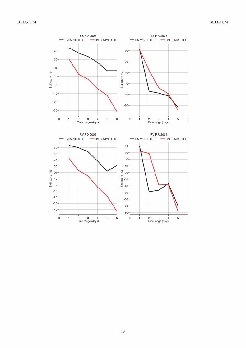
BELGIUM BELGIUM
13
DM WINTER FD
SS FD 2005 SS RR 2005DM SUMMER FD DM WINTER RR DM SUMMER RR
0 1 2 3Time range (days)
4 5 6 0 1 2 3Time range (days)
4 5 6
20
40
30
10
0
-10
-20
-30
Ski
ll sc
ore
(%) 10
0
-10
30
20
-20
Ski
ll sc
ore
(%)
DM WINTER FD
RV FD 2005 RV RR 2005DM SUMMER FD DM WINTER RR DM SUMMER RR
0 1 2 3Time range (days)
4 5 6 0 1 2 3Time range (days)
4 5 6
20
40
50
60
30
10
0
-10
-20
-30
-40
Ski
ll sc
ore
(%)
10
0
-10
20
-20
-30
-40
-50
-60
-70
-80
Ski
ll sc
ore
(%)

CROATIA CROATIA
14
Report on Verification of ECMWF Products in CroatiaJune 2006
By Zoran Vakula and Lovro Kalin, Meteorological and Hydrological Service
1. Summary of major highlights of use and verificationThe 12 UTC ECMWF products are widely used in the operational forecasting practice at the Croatian Met Service, particularlyfor medium- and long-range forecasts. The 00Z forecasts are used occasionally in the operations. At short range, ECMWFproducts are used together with Aladin Croatia and DWD GME/LAM.
Verification is made on a point - to - point basis. Synop data are compared against the nearest model grid point result withthe emphasis on temperature, precipitation and wind. Various scores are computed occasionally, but verification is still notfully operational.
2. Verification of products
2.1 Objective verification
2.2 Direct model output
(i) No regular verification is made for parameters in the free atmosphere.
(ii) Verification of local weather parameters is computed mostly from synop data, verified against nearest model grid point.
Fig. 1 and Fig. 2 show deterioration in the 2m min and max temperature forecast skill against increased forecast range,approaching zero skill for the period between D7 and D10.
The sampling is made for warmer (April to September) and colder (October to March) periods of the year in order to emphasisea better skill during the colder period, particularly for the minimum temperature forecast.
Fig. 1 Skill of 2m minimum temperature forecast (Zagreb Maksimir)

CROATIA CROATIA
15
Fig. 2 Skill of 2m maximum temperature forecast (Zagreb Maksimir)
Fig. 3 Bias of the 12-hour precipitation larger than 0 for Zagreb Maksimir
For precipitation, various scores are calculated: bias, Equitable Threat Skill Score (ETSS), Hansen-Kuipers skill score (KSS),Heidke skill score (HSS), etc.
Fig. 3 clearly shows an improvement over the last three years for the 12-hour forecast bias. Although still relatively high, ithas been reduced in the year 2005 (green line), and the daily cycle is significantly less marked.

CROATIA CROATIA
16
Fig. 4 The Hansen - Kuipers skill score for the 12-hour precipitation larger than 0 for Zagreb Maksimir
A deterioration of the Hansen - Kuipers skill score -(KSS) with forecast time is displayed in Fig. 4. -Towards the end of theforecast period some improvement is noticed, however, no explanation for such model performance could be offered.
The distribution of the forecasted wind speed (Fig. 5) is narrower than observed and shifted to the lower speeds. The frequenciesof lower wind speed are overestimated, and frequencies of higher wind speed are underestimated. This is a common featureto many models.
Fig. 6 displays correlation coefficient between the ECMWF forecast and observations. Up to D5 it is relatively stationarybetween 0.6 and 0.7 value. After D5 it decreases to below 0.3 value. It can be noticed that the average value and deviation ofthe forecast are significantly smaller than the observed values (represented on the y-axis). Such a result might have beeninfluenced, at least partly, by the positioning of the wind-measuring instrument – it is located at the top of the hill.
Fig. 5 Distribution of forecasted and observed wind speed frequencies for Split Marjan, located at the Adriatic coast, for 2005.

CROATIA CROATIA
17
Fig. 6 Average, standard deviation and correlation coefficient of forecasted and observed wind at Split Marjan for theyear 2005
(iii) Verification of the sea state, based on significant wave height forecast, is calculated regularly. However, the resultsare not presented in this report.
2.1.2 ECMWF model output compared to other NWP models
The ECMWF products are compared to the Aladin mesoscale model products, usually with the 00UTC Aladin Croatia runand the 00UTC Aladin Lace run (the latter has been recently terminated). For 2m temperature and precipitation, skill of theECMWF model over Croatia is found to be comparable to that of the Aladin model, at some locations showing even betterresults than Aladin (Figs. 7 and 8).
For wind forecast, Aladin is significantly more successful than the ECMWF model. This might be explained by the fact thata much higher Aladin horizontal resolution resolves better a complex orography in Croatia. Such a high model resolution ismatching better the episodes of intense local katabatic (bora) wind.

CROATIA CROATIA
18
Fig. 7 RMSE for 2m maximum temperature for the warmer part of the year.
Fig. 8 ETSS for the 24-hour precipitation for D2, with the thresholds of 0.1, 1 and 5 mm.

CROATIA CROATIA
19
2.1.3 Post-processed products
A simple linear regression equation (MOS) is applied to the 2m temperature forecast and precipitation probabilities based onstatistical assessment of the model input. They show some improvement when compared to DMO, however, they are not shownin this report.
An effort to introduce clustering of EPS on a new, reduced domain has recently been done. Clustering method is based onMetview macro developed at ECMWF. Beside standard clustering method, some other meteorological elements have beenused as clustering parameters (like specific humidity and thickness). The verification is yet to be done.
2.1.4 End products delivered to users
Based on ECMWF medium range, monthly and seasonal forecasts and combined with the analogue method, monthly forecastsfor temperature and precipitation anomalies are issued twice a month.
Based on the two different methods, verification of the Croatian Met Service monthly forecasts shows some skill and animprovement over past years - particularly when ECMWF forecasts were introduced and implemented: deterministic in year1995, EPS in 2000 and eventually seasonal forecasts.
2.1.5 Seasonal forecasts
ECMWF seasonal forecast is consulted regularly, particularly when issuing a seasonal forecast for Croatia - a new product inthe Met Service,. However, there is no regular objective verification of the model output.
2.1.6 Monthly forecasts
No objective verification of ECMWF monthly forecast is being done.
2.2 Subjective verification
No subjective verification is done operationally. It is planned that recently introduced operational daily report describing currentsynoptic situation and models’ performances will be a good basis for such verification.
Regarding seasonal forecasts, there is an impression that the signal in most of the cases is still too weak, though a systematicverification of seasonal forecasts is not being done.
3. ReferencesECMWF, 2005: Verification of ECMWF products in Member States and Co-Operating States, Report 2005
Nurmi, P., 2003: Recommendations on the verification of local weather forecasts, ECMWF Technical Memorandum No. 430,December 2003, 19 pp.
Wilks, D. S., 1995., Statistical Methods in the Atmospheric Sciences. Academic Press, London, 464 pp.

CZECH REPUBLIC CZECH REPUBLIC
20
Application and verification of ECMWF products in the Czech RepublicCzech Hydrometeorological Institute (CHMI)
1. Summary of major highlights of use and verificationThe Centre’s products have been widely used by the Central and Regional Forecasting Offices in the CzechHydrometeorological Institute for medium-range and to some extent also in short-range forecasting. The clusters, tubes, plumesand EPS-grams are considered in order to evaluate the credibility of the main deterministic forecast as well as to prompt forpossible scenarios in situations of low determinism. A certain experience of the Extreme Forecast Index and other probabilisticproducts has been obtained. The Centre’s graphical products available on the web server are used also by the Weather Serviceof the Czech Army.
The final medium-range forecasts produced by forecasters are currently used in the general weather forecasting for publicand state authorities in the national Warning and Alert Service.
Experimentally we began to use prediction of precipitation and temperature of deterministic model as an input to hydrologicalmodels to predict water levels in the rivers up to ten days ahead. These predictions were also used during spring floods linkedwith melting snow and rain at the end of March this year. Although the results were not very successful, it is possible to usethem qualitatively. Next time we plan to use 25% and 75% percentiles of precipitation from EPS to estimate the range ofprobable discharges in the rivers.
The seasonal and monthly forecasts are consulted in the long-range forecast process. Currently the results of bothdeterministic and ensemble forecast are used in the identification of the weather type for the weather-analogue-based forecastingmethod for monthly forecasting.
Three-dimensional wind forecasts over the Northern Hemisphere up to +120 h are used as the input to the trajectory modelused for the assessment of risk to the civil safety from remote nuclear or other accidents.
2. Verification of productsThere is currently no objective or systematic subjective verification of ECMWF products carried out. The general scorescalculated and published by ECMWF are considered informative. For now we also use verification of ECMWF products fromthe Green Book. Considering the character of medium-range weather forecasts, the verification scores from neighboringcountries are well applicable also for our service.
2.1 Objective verification
2.1.1 Direct ECMWF model output
2.1.2 ECMWF model output compared to other NWP models
2.1.3 Post-processed products
2.1.4 End products delivered to users
2.1.5 Seasonal forecasts
2.1.6 Monthly forecasts
2.2 Subjective verification
2.2.1 Subjective scores
2.2.2 Synoptic studies, evaluation of the behaviour of the model
2.2.3 Seasonal forecasts
2.2.4 Monthly forecasts
The seasonal and monthly forecast products are considered as having some informative value. The frequency of “no signal”of these forecasts is considered as still too high.
3. References to relevant publications

DENMARK DENMARK
21
Verification of ECMWF products at the Danish Meteorological Institute
1. Summary of major highlights In this years report objective verification results are presented for a series of with focus on operationally used products.
2. Verification of products
2.1 Objective verification
2.1.1 Direct ECMWF model output
2.1.2 ECMWF model output compared to other NWP models
Forecasts from ECMWF are used as boundary data for the DMI versions of HIRLAM. On a routine basis verification of 2 mtemperature and 10-metre wind are made against 27 synop stations. In Figure 1 the hit rate for the 2-metre temperature beingwithin two Kelvin is shown for 12 and 24-hour forecasts. ECH corresponds to the ECMWF model (extracted in 1 degreeresolution daily from MARS) and S05 is a 5 km HIRLAM model covering Denmark and the surrounding area.
Fig. 1 Hit rate for S05 HIRLAM models and the ECH (ECMWF) for 2-metre temperature. The threshold used is 2 Kelvinand 27 Danish stations are used for the verification covering the period 2005
Fig. 2 Hit rate for S05 HIRLAM models and the ECH (ECMWF) for 10-metre wind. The threshold used is 2 m/s and 27Danish stations are used for the verification covering the period 2005
Figure 2 shows the hit rate for the 10-metre wind being with in 2 m/s for 12 and 24-hour forecasts.

DENMARK DENMARK
22
2.1.3 Post-processed products
2.1.4 End products delivered to users
The quality and benefit from Kalman filtering at DMI are measured every third month. The Mean Error (ME) is calculatedfor both the Kalman filtered forecasts and the ECMWF forecasts using synop data. The difference between the absolute valueof these mean errors is calculated for forecast lengths +30, +54, +78, +102, +126, +150, +174, +198 and 222. The absolutevalue is introduced to avoid positive and negative mean errors cancelling each other. The mean error difference is then anestimate of bias correction, with negative values representing less bias in the Kalman filtered forecasts than in the ECMWFforecasts. This is shown for 2-metre maximum temperature in figure 3 upper graph for a number of Danish synop stationsidentified by their WMO number at the x-axes. Particularly large forecast lengths get a substantial bias correction. MEfck andMEmp in the title of figure 3 is mean error for respectively Kalman filtered forecast and EWMWF forecast.
In figure 3 lower graph corresponding Mean Absolute Error (MAE) differences are shown. Negative values represent lessmean absolute error in the Kalman filtered forecasts than in the ECMWF forecast, and this is the case for especially largeforecast length.
The same tendencies are recognized for other meteorological parameters such as wind speed.
The conclusion is that Kalman filtering is still profitable within the Danish area. It will be interesting to examine the evolutionof this quality and benefit measure of Kalman filtering as the models gets higher and higher resolution.
2MTX abs(MEfck)-abs(MEmp) – 2006 jan_mar
-3
-2.5
-2
-1.5
-1
-0.5
0
0.5
1
6019
6030
6031
6032
6041
6049
6051
6052
6056
6058
6060
6065
6068
6069
6070
6072
6073
6074
6079
6080
6081
6082
6088
6093
6096
6102
6104
6108
6109
6110
6116
6118
6119
6120
6123
6124
6126
6132
6135
6136
6138
6141
6149
6151
6154
6156
6159
6160
6168
6169
6170
6174
6179
6180
6181
6184
6186
6188
6190
6193
6197
base
30
54
78
102
126
150
174
198
222
2MTX MAEfck-MAEmp – 2006 jan_mar
-2.5
-2
-1.5
-1
-0.5
0
0.5
6019
6030
6031
6032
6041
6049
6051
6052
6056
6058
6060
6065
6068
6069
6070
6072
6073
6074
6079
6080
6081
6082
6088
6093
6096
6102
6104
6108
6109
6110
6116
6118
6119
6120
6123
6124
6126
6132
6135
6136
6138
6141
6149
6151
6154
6156
6159
6160
6168
6169
6170
6174
6179
6180
6181
6184
6186
6188
6190
6193
6197
2.1.5 Seasonal forecasts
The Danish Meteorological Institute produces both probabilistic and deterministic seasonal forecasts for the temperature inDenmark and southern Greenland (only probabilistic). The forecast lead is one month and the averaging period is three months.The probability forecast describes the probabilities for colder than normal, near normal, and warmer than normal and is basedon a purely statistical scheme using temperature in previous seasons as predictor. The deterministic forecast shows thetemperature anomaly and is based directly on the ECMWF dynamical forecast System 2. The skill of the deterministic forecastis highest in the spring. The forecasts are published in Danish on the DMI homepage on the Internet.
2.2 Subjective verification
3. References
Fig. 3

FINLAND FINLAND
23
Verification of ECMWF products at the Finnish Meteorological Instituteby Pertti Nurmi, Matias Brockmann and Juha Kilpinen
1. Summary of major highlightsThe operational end product verification system was in a halt for several months due to the moving of FMI to its new officebuilding and the entire computing environment (software and hardware) being heavily renewed. A new verification packageis under development. The entity-based field verification system announced in the previous Member State Verification Reportis close to reach an operational phase. It will be applied a.o. to the verification of precipitation forecasts associated withhydrological applications (Nurmi and Zingerle, 2006). Verification of post-processed ECMWF EPS products has remainedquite active in several studies focusing on the development of forecasts guidance applications to duty forecasters (Kilpinenet al., 2005). Operational verification of ECMWF output is, unfortunately, non-existent.
2.1 Objective verification
2.1.3 Post-processed products
The Scandinavian countries continued the joint project in an effort to define common criteria for producing warnings againstnear-gale-force winds in their adjacent sea areas (see, Verification Report, 2005). Figure 1 shows how Kalman filtering effectivelyremoves the negative bias in the ECMWF output, and Figure 2 the relation between the RMSE and the EPS mean spread forthis application. Figures 3 and 4 show some results of the various probabilistic methods being investigated. Regardless of theverification score (the Brier Skill Score, or the area under the ROC curve), all of the methods appear to be superior to directEPS in the first five-day forecast range. However, the order of superiority seems to change somewhat beyond c. Day 4.
2.1.4 End products delivered to users
Figures 5 thru 8 show selected results based on the end product verification dataset of FMI. Figures 5 and 6 demonstrate theevolution in quality during the past ten years. The temperature time-series (Figure 5) exhibit a predominant cold bias throughoutthe years, but also a positive trend in the reduction of the Mean Absolute Error during the latest years. For the Probability ofPrecipitation forecasts (Figure 6), the positive trend is indicated by the increase in the ROC area values: from c. 0.80 to 0.85,and from c. 0.75 to 0.80, for one-day and two-day forecasts, respectively. Figure 7 shows somewhat different temperature forecasterror behavior, during 2005, at three climatologically disparate stations in southern, central, and northern Finland, respectively.Finally, Figure 8 compares one-day and two-day Probability of Precipitation forecasts in 2005. There is a notorious over forecastingbias at both forecast ranges. Despite this, last year appears to be somewhat better than the previous five-year period on averageaccording to the Brier Skill Score. Also, the ROC curves and the absolute ROC area values appear to be quite satisfactory.
2.2 Subjective verification
The duty forecasters of the Weather Warning Service of FMI participated last year in a survey to subjectively evaluate thevarious NWP guidance products available to them (Brockmann et al., 2005). The forecasters, altogether 14 of them, wererequested to specify the principal guidance being used by them for one-day, two-day, and medium-range forecasts. Thereasoning for their choice of model was also asked. The main models available in this pilot study were the 22 km resolutionRCR-HIRLAM-00UTC run, the 9 km resolution MBE-HIRLAM-18UTC run, the ECMWF-12UTC run, the U.S. global GFS-00UTC run and the Polish model 00UTC run.
In general, it can be concluded that HIRLAM (RCR / MBE) and ECMWF were considered equally often as the principalguidance in the D+1 forecast range, while ECMWF was clearly preferred in the D+2 range and beyond (Figures 9 thru 11).There are various reasons why such results should be interpreted with some caution. About every other time the evaluationform was left totally unfilled. Quite often the forecasters could not differentiate between the quality of the models at all.ECMWF may have been occasionally preferred to preserve continuity throughout the entire forecast range. At the time of theevaluation, the usefulness of the fine-resolution MBE-HIRLAM was suffering from late delivery and relatively non-userfriendly visualization tools. And so on.
3. ReferencesMatias Brockmann, Ilkka Juga and Marianne Sågbom, 2005: Finnish duty forecasters’ evaluation of the Hirlam RCRforecasts in relation to other NWP guidance during the period 12.4.2005 - 22.9.2005, a pilot study. Internal report of the FMIWeather Warning Service.
Juha Kilpinen, Annakaisa Sarkanen, Pertti Nurmi and Sigbritt Näsman, 2005: Comparison of ECMWF and HIRLAMwind forecasts in the Baltic Sea. Proceedings, 10th ECMWF Workshop On Meteorological Operational Systems (ECMWF,14-18 November 2005). http://www.ecmwf.int/newsevents/meetings/workshops/2005/MOS10/index.html
Pertti Nurmi and Christoph Zingerle, 2006: Entity-based verification and uncertainty issues. Joint COST 731 and NetFAMWorkshop on Uncertainty in High-Resolution Meteorological and Hydrological Models (Vilnius, Lithuania, 26-28 April 2006).http://www.meteo.lt/vilnius/pro.html

FINLAND FINLAND
24
24
0
-0.1
-0.2
-0.3
-0.4ME
-0.5
-0.6
-0.7
-0.848 72 96 120 144
Mean Error (ME)
Lead time (hour)
opercontroleps meanKalman filtered oper
24
4.5
4
3.5
3
2.5
RM
SE
2
1.5
1
0.548 72 96 120 144
Root Mean Squared Error (RMSE)
Lead time (hour)
opercontroleps meanKalman filtered opereps mean spreadmean of indiv. eps members
Fig. 1 The Mean Error (ME) of wind speed forecasts asa function of forecast leadtime, averaged overfive Finnish coastal stations and four cold sea-sons, 2002-2005. The results are for the opera-tional ECMWF DMO (red curve), Kalman filteredforecasts (pink curve), the control run (greencurve) and the EPS mean (blue curve).
Fig. 2 As Figure 1, but for the Root Mean Square Error(RMSE). Here, the distributions of EPS meanspread and the mean of individual EPS membersare shown, for reference.
dep. calib. epscalib. epsmeancalib. eps spread
epsrec. calib. epsindep. error dress.dep. error dress.
12 24 36 48 60 72 84 96 108 120 132Lead time (Hour)
0.5
0.45
0.4
0.35
0.3
0.25
0.2
0.15
0.1
0.005
0
BS
S
Brier Skill Score (BSS) P (WS> 14m/s)1
0.95
0.9
0.85
0.8
0.75
0.712 24 36 48 60 72 84 96 108 120 132
ROC Area P (WS> 14m/s)
Lead time (Hour)
RO
C A
rea
dep. calib. epscalib. epsmeancalib. eps spread
epsrec. calib. epsindep. error dress.dep. error dress.
Fig. 3 The Brier Skill Score (BSS) of near-gale forecasts(wind speeds exceeding 14 m/s) for the samedata as in Figures 1 and 2. The ECMWF DMOEPS (pink line) is compared with six differentmethods to define the probabilistic distribution ofthe event: dependent error dressing - independenterror dressing – recursive calibration of the EPS –dependent calibration of the EPS – calibration ofthe EPS mean – calibration of the EPS spread.
Fig. 4 As in Figure 3, but for the area under the ROCcurve.

FINLAND FINLAND
25
Fig. 5 Evolution in time, 1995-2006, of the Mean Error (green curve), and the Mean Absoulte Error (magenta curve) of24 hour (upper) and 48 hour (lower) daytime maximum temperature forecasts, averaged over three Finnish inlandstations. The red numbers are annual averages of the Hit Rate (temperature forecasts correct within 2 degrees).
Fig. 6 Evolution in time, 1995-2006, of the Brier Skill Score over persistence (blue curve) and the area under the ROCcurve (pink curve) of 24 hour (upper) and 48 hour (lower) Probability of Precipitation forecasts, averaged overthree Finnish inland stations. Annual averages are indicated by numbers and solid dots.
Fig. 7 Box plots of 36 hour minimum temperature forecast errorsat three Finnish inland stations (Hki, Tre, Sod), in 2005.

FINLAND FINLAND
26
Fig. 8 Reliability diagrams (upper) and ROC (lower) of 24 hour (left) and 48 hour (right) Probability of Precipitation fore-casts, averaged over three Finnish inland stations in 2005. BS = Brier Score, SS_5a = BS improvement during2005 compared to the previous five years, SSpbs = Brier Skill Score over persistence in 2005.
Fig. 9 Subjective comparison of different NWP models available to FMI duty forecasters during a c. five-month periodin 2005, separately for one-day, two-day and three-to-five-day forecast range. RCR and MBA are the 22 km and9 km versions of HIRLAM, respectively, GFS is the U.S. global model.

FINLAND FINLAND
27
Fig. 10 Subjective comparison of different NWP models at forecast range D+1 during different months, April toSeptember, in 2005. Data coverage and notations as in Figure 9.
Fig. 11 As in Figure 10 but at forecast range D+2.

FRANCE FRANCE
Verification of ECMWF products at Météo-France
1.Summary of major highlights of use and verification
ECMWF products are widely used at all Météo-France forecast centres : T799 for the short-range forecast in addition to othermodels (the 2 production runs at 00 and 12 UTC are used) in order to choose the best option, and EPS from day 4 to day 7forecast to propose a scenario with confidence index linked to the number of tubes. The extension of the forecast range beyondday 7 is being studied, in order to produce bulletins for the general public out to day 9.
ECMWF monthly forecast is now used in operations.
ECMWF is used to start ARPEGE-Climat seasonal forecasts.
The forecasters from Meteo-France largely consult ECMWF web site products.
2. Application of products
2.1 Post-processing of deterministic model output
2.1.1 Statistical adaptations
Millions of local forecasts of weather parameters are produced daily through statistical adaptation of NWP output. Mainmethods are multiple linear regression (MLR) and linear discriminant analysis (DA). MOS (model output statistics) is generallypreferred to PP (perfect prognosis). Kalman filter (KF) is applied when relevant.
• 2m temperature: MLR+KFFrance: 2588 stations. +12h to +180h by 3h from 12 and 00UTC + daily extremes.world: 6010 stations. +6h to +180h by 3h + daily extremes from 12 and 00UTC.
• 10m wind speed and direction: MLRFrance: 811 stations. +12h to +180h by 3h from 12and 00UTC.
• Total cloud cover: MLR+KF: DA on 4 classesFrance: 150 stations. +12h to +180h by 3h from 12 and 00UTC
• 2m relative humidity: MLR+ KFFrance: 1156 locations in France, lead time: +12h to +180h by 3h + daily extreme from 12 and 00UTC
2.1.2 Physical adaptations, limited area modelling
2.1.2.1 Dispersion model
The dispersion and trajectory model MEDIA can be driven by ECMWF output.
2.1.3 Derived fields
(no application)
2.1.4 Other
2.1.4.1 Seasonal forecast
ECMWF daily analysis are used to define initial atmospheric conditions for the Météo-France seasonal ensemble forecast (9members). ERA15 is used to compute the renormalization (to observation) of seasonal forecast indices (T850 and Z500).
ERA15 and ECMWF analysis are used to compute monthly and seasonal climate anomalies disseminated by an internalweb page. These anomalies are used to perform a subjective verification of our seasonal forecast.
ECMWF seasonal forecast are used monthly to assess the confidence of the seasonal forecast from Météo-France. All theseasonal information available on the web page (Ocean analysis, ocean forecast, atmospheric forecast, forecast indices, ...)are checked monthly as additional input and verification for the M-F forecast (subjective comparison) and to compare thebehaviour of forced versus coupled ensemble forecast.
A climate bulletin is monthly edited taking into account available information on the state of the climate system and providinga consensual seasonal forecast based on products from different centres (including ECMWF). Note that this bulletin is forinternal purpose and that a monthly briefing is planned in the future. However, ACMAD (Niamey) has asked to receive anddisseminate it. An end-user bulletin is updated monthly and sent to partners for a pilot experiment.
The coupled version of the Météo-France model is evaluated in the frame of the Demeter experiment. This model could beincluded in the Demeter multi-model ensemble planned at ECMWF and could be used at Météo-France in operational modein the future.
28

FRANCE FRANCE
29
2.1.4.2 Local fields storage
ECMWF model fields are stored in a local and operational data base for a few days.
2.1.4.3 Tropical region aspects
ECMWF model provides a particularly useful forecast guidance in French tropical regions and for cyclone forecasting.
2.2 Post-processing of EPS output
2.2.1 Statistical adaptations
Statistical adaptation is applied to individual ensemble runs. Methods are the same as for the deterministic model output (see2.1.1) but pseudo-PP (statistical equations computed during the first 24 hours then applied to the other corresponding steps)is preferred to MOS.
Ensemble mean :
• 2m temperature: MLR+KFFrance: 1206 stations. +12h to +240h by 3h from 12 and 00UTC + daily extremes.world: 3339 stations. +6h to +240h by 3h + daily extremes from 12 and 00UTC.
• 10m wind speed : MLRFrance: 586 stations. +12h to +240h by 3h from 12and 00UTC.
Probabilities and distributions :
Ensemble distributions are calibrated before computing probabilities. The method of calibration is based on the use of rankdiagram statistics (e.g. Hamill and Colucci 1998). A new method, the Bayesian Model Averaging developped at Unviversityof Washington (see Raftery et al, 2005) will be used in the future.
• 2m temperature, probabilities: MLR applied to individual runs, ensemble calibration.France: 1206 stations. Daily extremes day+1 to day+8.
• 10m wind speed, probabilities (40/70/100km/h): MLR to individual runs, ensemble calibration.France: 586 stations. +0h to +240h by 6h from 12 and 00 UTC.
• 24h precipitations, probabilities (occurrence): ensemble calibration.France: 1206 stations. day+1 to day+8 from 12 and 00 UTC.
2.2.2 Graphics
Forecasters of the national and regional centres visualize ECMWF outputs (deterministic model, EPS and wave model) throughthe SYNERGIE system implemented on workstations. They can daily compare ECMWF output to other models outputs andchoose a scenario based on ARPEGE, Unified Model of the Met Office ECMWF, or mix for the short range forecast.
The EPS is daily used in the Medium-Range forecast guidance through the tubing classification. The most probable forecastis given by the central cluster mean in terms of weather type. The confidence index is directly linked to the number of tubesbut subjectively fixed by the forecaster.
Other graphical products are available for the forecasters in order to detect extreme phenomena like deep cyclones, strongconvection from the EPS members.
The general flow orientation and wind speed over 3 basins (North-Sea, NE-Atlantic and Mediterranean sea) is evaluated inthe marine Medium-Range forecast, looking at EPS-based wind roses. The marine forecasters produce a medium-range bulletin.
In the tropical areas (French West Indies, La Réunion, New-Caledonia, French Polynesia), the EPS is used for cyclonetracking (strike-probability maps). La Réunion is a Regional Specialised Meteorological Centre, it is responsive for cycloneforecasting in the southwest Indian Ocean.
Furthermore several EPS-based charts are produced on the tropical areas for the daily forecasts: MSLP spaghettis, ensemblemean of MSLP and Theta’w at 850hPa, probability that Theta’w at 850hPa is greater than 20 and 22°C, probability that CAPEis greater than 1000 and 2000 J/kg, EPSgram with fixed y-axis for the 6h-precipitations.
Products based on Wave EPS are also very useful: probability of swell height greater than 3m, which is a pertinent dangerthreshold, EPSgram of total swell height (as plotted on the figure 1), wave roses.

FRANCE FRANCE
30
2.3 Use of monthly forecasts
Since January 2006, the forecasters from the national centre produce a weekly bulletin for a specific user. The bulletin is basedon the products available on ECMWF web server: probabilities of T2m anomaly, multiparameter outlook, weather regimesclusterisation, Hovmoeller diagram... The Bulletin describes the evolution of general flow, the consistency of the model andfocuses on the temperature anomalies.
2.4 Use of end products
• Products for International Desk of Météo-France
Europe media weather (daily): T799 till D4 (together with ARPEGE), ensemble D5/D6 : central cluster from tubing, rainprobabilities, T850 anomaly probabilities. Worldwide forecast (private consultancy): T799 (0.5), ensemble mean, rainprobabilities, EPSgram, EFI.
3. Verification of products
3.1 Objective verification
3.1.1 Direct ECMWF model output
ECMWF model is compared to soundings, SYNOP and analyses (ARPEGE and ECMWF).
3.1.2 ECMWF model output compared to other NWP models
3.1.2.1 Daily control
Ensemble mean is compared to the control run and the operational run.
3.1.2.2 Analysis as a neutral reference
ECMWF analysis is used as a neutral reference to compute ARPEGE and its test suite scores so that they can be compared.
3.1.2.3 Composite score
We use a composite score, the difference between ARPEGE-model rmse (over EUROPE against soundings and over NorthernHemisphere against analysis for 24H and 72H forecast range) and the rmse of DWD, UKMO and ECMWF models.
3.1.2.4 Wave model
A comparison between ECMWF wave model and Météo-France wave model is done over the Atlantic Ocean. This comparisonis carried out for the SWH against buoys and analysis. Against buoys and over the western region, ECMWF wave model looksbetter (there is a strong positive bias for Météo-France model). Over the eastern region performances are quite similar (althoughone can note a small negative bias in this region for both models).
Fig. 1 EPSgram of total swell height on Bora-Bora. EPS from 20060413 0h.

FRANCE FRANCE
3.1.3 Post processed products
We use ECMWF scores sent to WMO and other numerical centres in comparison with the scores computed with our procedures.Small differences can be explained by the soundings selection system or the grid resolution used.
3.2 Subjective verification
3.2.1 Subjective scores
3.2.1.1 Short range verification
Forecasters at the national centre perform a daily subjective verification of the short-range forecasts. A note is given to ARPEGEand to ECMWF model. Moreover, the differences in the North Atlantic Ocean and Europe regions are checked every daybetween UKMO, Météo-France and ECMWF forecasts and reported if they are important. A verification is performed at thevalidity date of the forecasts. The reference for the verification can be either the analyses of the models or in situ observations.
3.2.1.2 Monthly forecast verification
Since the monthly forecasting system has been used in operations, the forecasters have assessed the T2m anomaly forecastsover France. For every week, the notations vary between A (good) and D (bad). The figure 2 plots the proportion of eachnotation for week 1 to week 4, over a sample of 20 members.
31
Fig. 2 Repartition of subjective notations for monthly T2m anomaly over France (sample size=20).
Nombre total de A
Nombre total de B
Nombre total de C
Nombre total de D
S-1
S-3 S-3
S-2
3.2.2. Evaluation of the behaviour of the EPS
3.2.2.1.Synoptic assessment
Forecasters go on evaluating EPS outputs. Automated forecasts use the probabilistic approach, however weather reports issuedby the forecasters are mainly based on the interpretation of the central cluster of the tubing method. This has been found tobe the best method to produce the deterministic part of the medium-range forecasts.
Subjective evaluations therefore aim at measuring the ability of the central cluster to predict large scale (“supra-synoptic”scale) flow types above western Europe. Table 1 indicates the percentage of good forecast over the last years of our mediumrange forecasts.

FRANCE FRANCE
4. ReferencesHamill, T. M., and S. J. Colucci, 1998 : Verification of Eta-RSM ensemble probabilistic precipitation forecasts. Mon. Wea.Rev., 126, 711-724.
Raftery, A.E., Gneiting, T., Balabdaoui, F. and Polakowski, M. (2005). Using Bayesian Model Averaging to CalibrateForecast Ensembles. Monthly Weather Review, 133, 1155-1174.
32
Year D+4-D+5 D+6-D+7
2005 76 55
2004 86 61
2003 86 66
2002 83 57
Table 1 Percentage of good medium range forecast over western Europe

GERMANY GERMANY
Verification of ECMWF products at the Deutscher Wetterdienst (DWD)By Martin Göber
1. Summary of major highlights of use and verificationSince 2004 a MOS interpretation of the ECMW model (ECMOS) has been used operationally in addition to the traditionalMOS of DWD’s global model GME (GMOS). A weighted average of the two MOS’ forms MOS/MIX - the best availableguidance for the production of local short and medium range forecasts. The introduction of MOS/MIX has lead to a furthersubstantial increase in forecast accuracy.
ECMWF’s high resolution model is always used together with other models in short- and medium-range forecasting. Formedium range forecasting the EPS is used additionally; in the short range the LEPS (Local model nested into EPS clusters)provides ensemble information.
Since a long history at DWD of the verification of medium range forecast has consistently shown that the forecasters cannot improve on MOS/MIX on average, the separate verification of the human forecasts has been discontinued.
Since December 2003 T+12 forecasts over the oceans from the ECMWF model have been assimilated into the GME modelas so called „pseudo temps”.
2. Application of ProductsThe high resolution ECMWF model forms together with DWD’s model GME the general operational data base. Both forecastsare statistically interpreted up to 7 days in terms of near surface weather elements by means of a PPM scheme (AFREG) aswell as by MOS and subsequent averaging of the two interpretations to form „AFREG/MIX” and “MOS/MIX”.
EPS products are used intensively in order to create a daily simple confidence number and describe alternative solutions.Furthermore, they are used to estimate the prospect for extreme weather events.
3. Verification of products
3.1 Direct ECMWF model output
Upper air forecasts from ECMWF continued to exhibit smaller errors than DWD-GME forecasts (Fig. 1). The RMSE of theECMWF model for 500hPa geopotential height has decreased by more than 2% (0,4 gpm) in the short range from 2004 to2005 and by about 3% for the GME. ECMWF MSLP error growth with forecast range is about one day better than for DWD-GME, which translates into an advantage of about 18 hours in terms of availability of the forecast. The RMSE’s of the ECMWFand GME model for MSLP have decreased in 2005 by about 0,1 hPa, but so has the RMSE of the persistence forecast, i.e. noincrease in skill has been noted.
33
Fig. 1 RMSE 500hPa geopotential over Europe. DWD(Numerical Weather Prediction model GME),EC (high resolution ECMWF model), persist-ence (analysis from the initial state is used asa forecast for all following days), climate (longterm mean of the predictand (H500, MSLP)serves as a constant forecast).
0
20
40
60
80
100
120
140
160
0 1 2 3 4 5 6 7 8 9 10
days ahead
rmse
[gpm
]
ECDWD
persistence
climate
H500 hPaEurope
12/04 - 11/05

GERMANY GERMANY
3.1.3.1 Post-processed products PPP
Here, various statistically post-processed model forecasts are compared for the following:
Predictands
MIN = daily minumum temperature (°C)MAX = daily maximum temperature (°C)SD = daily relative sunshine duration (%)dd = surface wind direction (°) 12 UTC. Only verified, if ff(obs) ≥ 3 m/sff = surface wind speed (m/s) 12 UTCPoP = Probability of Precipitation > 0 mm/dPET = potential evapotranspiration (mm/d)RR = a binary predictand: precipitation amount > 0 mm/d: Yes/No;
Forecast Types
AFREG/MIX = Post processed product AFREG(MIX) = AFREG(EC)+AFREG(DWD)/2EC = high res. ECMWF model, DWD = operational DWD Global Model “GME” (initial time: 00 UTC). PPP is generated for several areas of the whole Germany, but verified against point observations at 6 stations.
MOS/MIX = PPP, a weighted average of Model Output Statistics MOS/GME and MOS/EC
and Verification measuresrmse is used for both categorical and probabilistic forecasts (equals square root of the Brier Score)RV = Reduction of Variance against reference, 1-(rmse/rmse*)2, here: mean value for day 2 ... 7rmse* = smoothed climate as the best reference forecast to evaluate forecast skillHSS = Heidke Skill Score, only for binary predictandsHSS = mean value for day 2 ... 7
34
Fig. 2 Same as fig. 1, but for RMSE of mean sealevel pressure.
0
2
4
6
8
10
12
0 1 2 3 4 5 6 7 8 9
days ahead
rmse
[hP
a]
EC
DWD
persistence
climate
MSLPEurope
12/04 - 11/05

GERMANY GERMANY
The skill (RV) of the forecasts in 2005 was better than 2004 for all variables. An increase of 2-13% RV was found for maximumtemperature and precipitation, specifically for the short range. MOS/MIX forecasts have substantially smaller errors thanAFREG/MIX, which is only partly due to the lower (and thus less realistic) variability of MOS forecasts. The lower variabilityof MOS, especially in the medium range, is an obstacle for the use of it for forecasts of more severe weather. Here, the morevariable solutions of the EPS serve as an important additional guidance.
Figs. 4–5a,b show two things: i) the MOS technology performs better than a perfect prog technology (AFREG) ; ii) mixingPP from both models leads to an improvement of the forecast, especially in the medium range.
35
Table 1 Verification of operational medium range forecasts for 6 stations in Germany (Hamburg, Potsdam, Düsseldorf,Leipzig, Frankfurt/M., München), 01/05- 12/05. Day of issue = day +0 = today at noon.1)Here, persistence is used as a ‘reference forecast’.
rmse day
+2 +3 +4 +5 +6 +7 +8
rmse*
(climate) RV(%)
MIN AFREG/MIX 2,32 2,43 2,60 2,80 3,06 3,37 3,654,01
56
MOS/MIX 1,67 2,00 2,26 2,60 2,89 66
MAX AFREG/MIX 2,35 2,57 2,85 3,15 3,56 3,89 4,144,66
61
MOS/MIX 1,89 2,27 2,67 3,01 3,35 67
SD AFREG/MIX 25,8 26,2 27,4 28,8 30,3 31,1 32,0 32,2 23
dd1) AFREG/MIX 44,2 47,1 54,1 62,8 70,5 76.1 81,391,4
62
dd1) MOS/MIX 33,7 39,9 49,4 60,1 69,4 69
ff AFREG/MIX 1,67 1,82 1,89 2,05 2,16 2,21 2,212,19
23
MOS/MIX 1,52 1,72 1,84 1,97 2,03 31
PoP PPP 36,5 37,3 39,7 41,8 44,2 46,2 47,746,5
30
34,8 37,3 39,7 42,2 31
PET PPP 0,750 0,763 0,808 0,851 0,896 0,929 0,950 0,954 23
HSS% HSS
RR AFREG/MIX 56 53 46 40 29 24 180
49
MOS/MIX 64 56 48 37 51
Fig. 3 Reliability diagram (6 stations, year 2005, day+2... day+7; only up to day+5 for MOS(MIX))
Fig. 4 Forecast skill RV for Daily Mean Temperature(DWD, 6 stations, 2005)
0
20
40
60
80
100
0 20 40 60 80 100
forecasted probability (%)
obse
rved
rela
tive
frequ
ency
(%)
AFREG/MIX
idealMOS/MIX
PoP > 0 mm/d
-20
0
20
40
60
80
100
0 1 2 3 4 5 6 7 8 9 10
days ahead
RV
% (r
elat
ive
to c
limat
e)
AFREG/EC
PPP-AFREG/MIX
AFREG/GME
MOS/MIX
MOS/EC Daily Mean
Temperature

GERMANY GERMANY
3.1.3.2 EPS verification
EPS products are only verified in a PP form as a Kalman filtered mean of the ensemble for continuous variables and as arelative frequency for probability forecasts, respectively. The verification is done against point observations from Synop’s.
Up to 3 days ahead, MOS(MIX) presents by far the best guidance. In the medium range, AFREG(MIX) is of similar qualitycompared to MOS(MIX) for maximum temperature, whereas the Kalman-filtered EPS is most suitable as an additional guidancefor wind speed, cloud cover forecasts and latterly maximum temperature(Fig. 6). Maximum temperature forecasts from theEPS mean were 2 days better than in the past for the short range and one day in the medium range.
Probability of YES/NO precipitation forecasts continued to slightly underestimate the PoP, with MOS(MIX) exhibiting thebest resolution followed by AFREG(MIX) (Fig. 8). Stronger events (>5mm/d, Fig. 7) were hardly ever forecasted from theEPS, which is only partly attributable to the mismatch between areal precipitation forecasts and point observations. MOS(MIX)achieved a good calibration for this rather rare event.
36
Fig. 5a Forecast skill RV as a function of range, averagedfor all predictands taken in table 1(without PET and RR)
Fig. 5b follows from fig. 5a: a) Blue line: RV(AFREG/MIX) - RV(AFREG/EC)b) Claret red line: RV(MOS/MIX) - RV(MOS/EC)
-20
-10
0
10
20
30
40
50
60
70
0 1 2 3 4 5 6 7 8 9 10days ahead
RV
%
AFREG/MIXAFREG/ECMOS/MIXMOS/EC
-10-8-6-4-202468
10121416
0 1 2 3 4 5 6 7 8 9 10days ahead
RV
diff
eren
ce%
a)
b)

GERMANY GERMANY
Fig. 6 DMO(EPSmean)+KAL (pink) versus AFREG-MIX (blue) and MOS/MIX (magenta), dotted line = rmse(climate).
Sample: 01/05 - 12/05, DWD (5 stations).The EPS forecast for cloud cover, wind speed ff and maximum temperatureMAX is the arithmetical mean of all 51 ensemble members. PoP forecast is the relative frequency of the “yes-event forecast”. Notice, rmse is identical to SQR(BS), BS = Brier Score.
37
1,1
1,3
1,5
1,7
1,9
2,1
2,3
2,5
0 1 2 3 4 5 6 7 8 9days ahead
rmse
[m/s
]
ff (00 UTC)
18
20
22
24
26
28
30
32
0 1 2 3 4 5 6 7 8 9days ahead
rmse
[%]
Cloud cover
(12 UTC)1,4
1,9
2,4
2,9
3,4
3,9
4,4
4,9
0 1 2 3 4 5 6 7 8 9days ahead
rmse
[K]
c limate
AFREG/MIX
EPSmean
MOS/MIX
MAX
25
28
31
34
37
40
43
46
49
52
0 1 2 3 4 5 6 7 8 9days ahead
rmse
[%]
PoP > 0 mm/d
25
28
31
34
37
40
43
46
49
52
0 1 2 3 4 5 6 7 8 9days ahead
rmse
[%]
PoP > 5 mm/d
1,1
1,3
1,5
1,7
1,9
2,1
2,3
2,5
0 1 2 3 4 5 6 7 8 9days ahead
rmse
[m/s
]
ff (12 UTC)

GERMANY GERMANY
38
Fig. 7 Reliability of PoP forecasts by EPS (red), AFREG/MIX (blue) and MOS/MIX 5 stations, day +2 ... +7, (MOS/MIXonly up to day+5)
0
10
20
30
40
50
60
70
80
90
abscissa as left
rela
tive
freq
uenc
y of
fore
cast
s is
sued
% AFREG/MIX
EPSmean+KAL
MOS/MIX
0
20
40
60
80
100
0 20 40 60 80 100
probability forecast %
rela
tive
freq
uenc
y ob
serv
ed %
IdealAFREG/MIXEPSmean+KALMOS/MIX
PoP > 5 mm/d
rel. AFREG/MIX = 1.4rel. EPSmean+KAL = 8,5rel. MOS/MIX = 3,7
0
10
20
30
40
50
60
70
80
90
abscissa as left
rela
tive
freq
uenc
y of
fore
cast
s is
sued
%
AFREG/MIX
EPSmean+KAL
MOS/MIX
0
20
40
60
80
100
0 20 40 60 80 100
probability forecast %
rela
tive
freq
uenc
y ob
serv
ed %
PoP > 0 mm/d

GREECE GREECE
39
Verification of ECMWF Products in GreeceHellenic National Meteorological Service (HNMS) – P. Fragkouli, A. Mamara, T. Andreadis, I. Papageorgiou
1. Summary of major highlightsThe IFS deterministic model output (both 12.00 Z and 00. 00Z run) is used in HNMS as plotted fields mainly in the NationalForecasting Centre for medium range prediction. Also, from summer 2005, it is used as initial conditions for the Local AreaModel LM-COSMO.
2. Verification of Products
2.1 Objective Verification
2.1.1 Direct ECMWF Model Output
2.1.2 ECMWF model compared to other NWP models used by HNMS
The 12-h accumulated precipitation for both ECMWF’s and LM’s models (00.00 Z run) is verified against 7 synoptic weatherstations, up to 48 hours.
The non-hydrostatic Lokal Modell (LM) has been developed by the COSMO Consortium. It has a grid resolution of 0.0625(with centre point at 38(N, 24(E covering all the Greek territory, as well as part of the neighbouring countries. The prognosticfields are produced for a 48h range. The 00.00 Z run is using initial conditions from GME global model of the DWD.
The 7 synoptic weather stations (indicated in the maps below with their WMO location indicator) have been selected asrepresentative of all the main Greek regions. (16622 Thessaloniki, 16641 Kerkira, 16667 Mitilini, 16741 El. Venizelos, 16716Helliniko, 16749 Rhodos and 16754 Heraklion).
The LM-COSMO point-precipitation forecasts are the interpolated value from the nearest 9 points, while the ECMWF point-precipitation forecasts use the nearest to the selected points.
Figure 1 shows the annual Mean Error for 2005 of the 12-h accumulated precipitation forecasts of the ECMWF and LM-COSMO at the points of the 7 synoptic stations. In general, the results reveal that the LM-COSMO is overestimating theprecipitation amount for all the three 12-h forecasts compared with the corresponding ECMWF forecasts.
Using a 4x4 contigency table, the precipitation forecasts were verified at the ranges ≤ 0.2 mm, (0.2-2.5] mm, (2.5-10.0]mm, >10.0 mm and the scores Frequency Bias (FBIAS), Proportion Correct (PC), Probability of Detection (POD), False AlarmRatio (FAR), Threat Score (TS) has been calculated for all the 7 synoptic stations. Although the scores of both models arequite close, again the ECMWF forecasts have better performance.
The Tables below are showing the contingency tables and the scores for year 2005 for 3 synoptic stations (16622, 16741,16749) and for the second 12-h of accumulated precipitation.
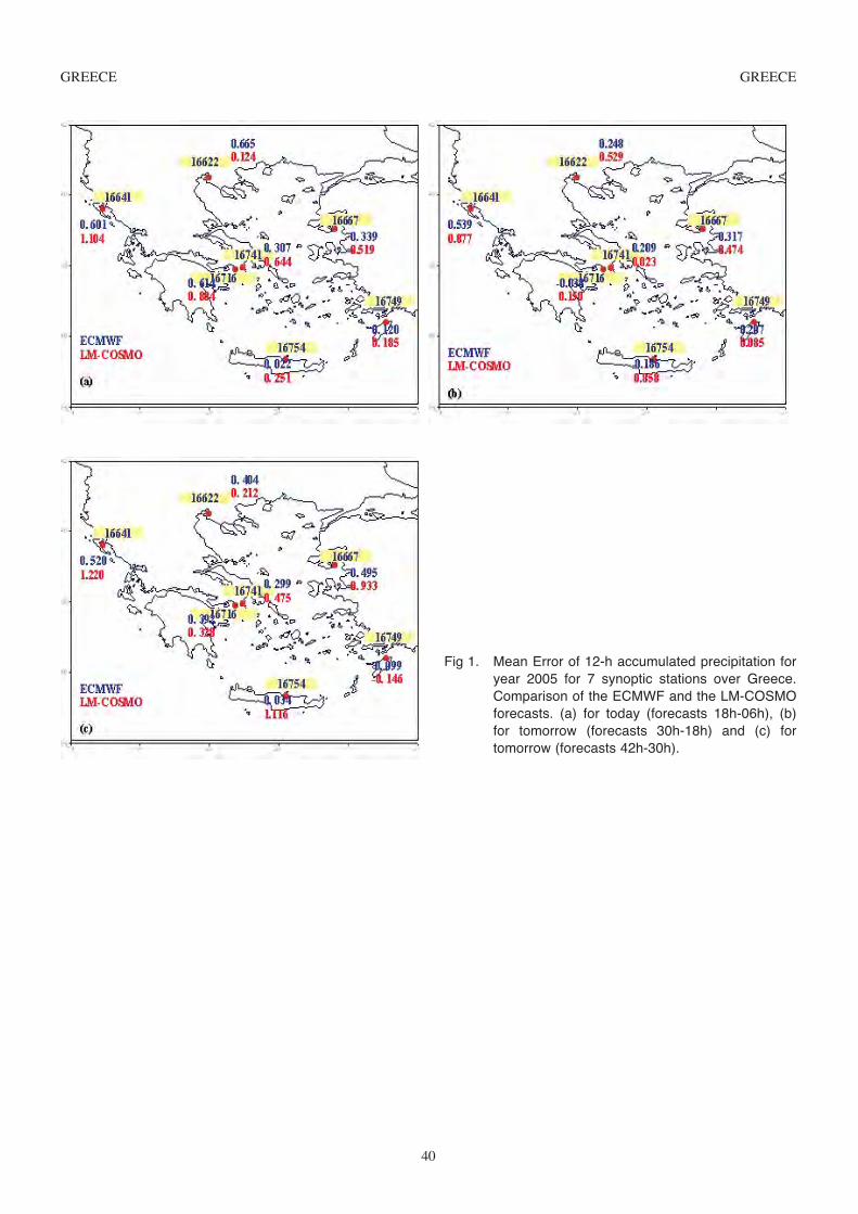
GREECE GREECE
40
Fig 1. Mean Error of 12-h accumulated precipitation foryear 2005 for 7 synoptic stations over Greece.Comparison of the ECMWF and the LM-COSMOforecasts. (a) for today (forecasts 18h-06h), (b)for tomorrow (forecasts 30h-18h) and (c) fortomorrow (forecasts 42h-30h).

GREECE GREECE
41
16622 – THESSALONIKI ECMWF forecast: (00Z+30h – 00Z+18h)
observation
≤ 0.2 mm (0.2-2.5] mm (2.5-10.0] mm >10.0 mm Σfct
fore
cast
≤ 0.2 mm 253 7 1 0 261
(0.2-2.5] mm 45 8 6 1 60
(2.5-10.0] mm 19 6 5 1 31
>10.0 mm 0 0 3 1 4
Σobs 317 21 15 3 356
≤ 0.2 mm (0.2-2.5] mm (2.5-10.0] mm >10.0 mm
FBIAS 0.823 2.857 2.067 0.997
PC 0.798 0.817 0.899 0.986
POD 0.798 0.381 0.333 0.992
FAR 0.031 0.867 0.839 0.006
TS 0.778 0.110 0.122 0.986
16622 – THESSALONIKI LM-COSMO forecast: (00Z+30h – 00Z+18h)
observation
≤ 0.2 mm (0.2-2.5] mm (2.5-10.0] mm >10.0 mm Σfct
fore
cast
≤ 0.2 mm 255 8 4 0 267
(0.2-2.5] mm 48 6 5 0 59
(2.5-10.0] mm 13 6 3 1 23
>10.0 mm 1 1 3 2 7
Σobs 317 21 15 3 356
≤ 0.2 mm (0.2-2.5] mm (2.5-10.0] mm >10.0 mm
FBIAS 0.842 2.810 1.533 0.989
PC 0.792 0.809 0.910 0.983
POD 0.804 0.286 0.200 0.986
FAR 0.045 0.898 0.870 0.003
TS 0.775 0.081 0.086 0.983
Table 1 Contigency Table and Scores for the second 12-h of accumulated precipitation forecasts against observations forsynoptic station of Thessaloniki. (upper table): ECMWF performance, (lower table): LM-COSMO performance.

GREECE GREECE
42
Table 2 Contigency Table and Scores for the second 12-h of accumulated precipitation forecasts against observations forsynoptic station of El. Venizelos. (upper table): ECMWF performance, (lower table): LM-COSMO performance.
16741 - EL. VENIZELOS ECMWF forecast: (00Z+30h – 00Z+18h)
observation
≤ 0.2 mm (0.2-2.5] mm (2.5-10.0] mm >10.0 mm Σfct
fore
cast
≤ 0.2 mm 264 2 1 0 267
(0.2-2.5] mm 48 7 3 0 58
(2.5-10.0] mm 14 3 4 3 24
>10.0 mm 1 2 1 3 7
Σobs 327 14 9 6 356
≤ 0.2 mm (0.2-2.5] mm (2.5-10.0] mm >10.0 mm
FBIAS 0.817 4.143 2.667 0.997
PC 0.815 0.837 0.930 0.980
POD 0.807 0.500 0.444 0.989
FAR 0.011 0.879 0.833 0.009
TS 0.800 0.108 0.138 0.980
16741 - EL. VENIZELOS LM-COSMO forecast: (00Z+30h – 00Z+18h h)
observation
≤ 0.2 mm (0.2-2.5] mm (2.5-10.0] mm >10.0 mm Σfct
fore
cast
≤ 0.2 mm 286 5 2 1 294
(0.2-2.5] mm 30 5 4 2 41
(2.5-10.0] mm 11 2 0 2 15
>10.0 mm 0 2 3 1 6
Σobs 327 14 9 6 356
≤ 0.2 mm (0.2-2.5] mm (2.5-10.0] mm >10.0 mm
FBIAS 0.899 2.929 1.667 1.000
PC 0.862 0.874 0.933 0.972
POD 0.875 0.357 0.000 0.986
FAR 0.027 0.878 1.000 0.014
TS 0.854 0.100 0.000 0.972

GREECE GREECE
43
16749- RHODOS ECMWF forecast: (00Z+30h – 00Z+18h)
observation
≤ 0.2 mm (0.2-2.5] mm (2.5-10.0] mm >10.0 mm Σfct
fore
cast
≤ 0.2 mm 280 1 0 0 281
(0.2-2.5] mm 33 3 2 0 38
(2.5-10.0] mm 10 5 8 2 25
>10.0 mm 0 0 7 5 12
Σobs 323 9 17 7 356
≤ 0.2 mm (0.2-2.5] mm (2.5-10.0] mm >10.0 mm
FBIAS 0.870 4.222 1.471 0.986
PC 0.876 0.885 0.927 0.975
POD 0.867 0.333 0.471 0.980
FAR 0.004 0.921 0.680 0.006
TS 0.864 4.222 0.235 0.974
16749- RHODOS LM-COSMO forecast: (00Z+30h – 00Z+18h)
observation
≤ 0.2 mm (0.2-2.5] mm (2.5-10.0] mm >10.0 mm Σfct
fore
cast
≤ 0.2 mm 298 4 3 0 305
(0.2-2.5] mm 18 3 2 1 24
(2.5-10.0] mm 4 2 7 2 15
>10.0 mm 3 0 5 4 12
Σobs 323 9 17 7 356
≤ 0.2 mm (0.2-2.5] mm (2.5-10.0] mm >10.0 mm
FBIAS 0.944 2.667 0.882 0.986
PC 0.910 0.924 0.949 0.969
POD 0.923 0.333 0.412 0.977
FAR 0.023 0.875 0.533 0.009
TS 0.903 0.100 0.280 0.969
Table 3 Contigency Table and Scores for the second 12-h of accumulated precipitation forecasts against observationsfor synoptic station of Rhodos. (upper table): ECMWF performance, (lower table): LM-COSMO performance.
2.1.3 Post-Processed Products
2.1.4 End Products Delivered to Users
2.1.5 Seasonal Forecasts
2.2 Subjective Verification
3. References

HUNGARY HUNGARY
44
Verification of ECMWF products in Hungary
1. Summary of major highlightsThe objective and subjective verification of ECMWF deterministic (and ensemble) products has been continued as in previousyears. Some new methods were applied for deterministic, ensemble and seasonal forecasts as well. A new objective verificationsystem (called OVISYS as Objective Verification System) had been developed for the inter-comparison of several numericalmodels operationally used at the Hungarian Meteorological Service.
2. Verification of Products
2.1 Objective verification
2.1.1 Direct ECMWF model output
(i) in the free atmosphere
(ii) local weather parameters for locations
The objective verification has been performed by our Objective Verification System (OVISYS). This is an interactive web-based system with an underlying software. Users can define their verification requests on the web page and then the programsin the background compute the required statistical scores and display them in the chosen graphical representation on one ormore figures. This verification is based on the comparison of observations with forecast values interpolated (with bilinearinterpolation) to the observation locations. In the recent verification study the 00 and 12 hours runs of ECMWF model wasverified against all the Hungarian SYNOP observations for the whole 2005 year. The input forecast values for ECMWF weretaken from a 0.5°x0.5° post-processing grid. The verification was performed for the following variables:
• Total cloudiness
• 10m wind speed
• 2m temperature
• Minimum and maximum 2m temperature
• Daily accumulated amount of precipitation
BIAS and RMSE scores 48 and 168 hours are computed. The computed scores are presented on Time-TS diagrams (with theforecast range on the x-axis) (Fig. 1-9.).
Total cloudiness:
Fig. 1 RMSE and BIAS values for ECMWF total cloudiness forecasts for Hungary. There is a cloudiness underestima-tion at all ranges (around -5 and -10 percent). The RMSE values are slightly increasing along the forecastranges.

HUNGARY HUNGARY
45
Fig. 2 RMSE and BIAS values for ECMWF 10m wind speed forecasts for Hungary. The RMSE values are rather con-stant until the third day, then there is a slight increase afterwards. The BIAS fluctuates in a diurnal cycle at arange of about 0.5 m/s.
10m wind speed:
2m temperature:
Fig. 3 RMSE and BIAS values for ECMWF 2m temperature forecasts for Hungary. The RMSE values are slightlyincreasing with the forecast range and the BIAS fluctuates between -1 and 1 with a strong diurnal cycle.
Fig.4 Comparison of BIAS and RMSE values for daily minimum (left) and maximum (right) temperature for ECMWF 00and 12 UTC runs. The scores show that the models overestimate the minimum temperature and underestimatethe maximum temperature.
2m minimum and maximum temperature

HUNGARY HUNGARY
46
Fig. 5 Comparison of RMSE (left) and BIAS (right) values for daily accumulated amount of precipitation for ECMWF 00UTC and 12 UTC runs (valid for the second forecasted day, i.e. between 30h-54h 18h-42h respectively). TheECMWF model underestimates the precipitation quantity.
Precipitation:
2.1.2 ECMWF model output compared to other NWP models used by the HMS
The newly developed OVISYS system makes possible to inter-compare the performance of different numerical weatherprediction models. Hereafter the ECMWF and ALADIN/HU models will be compared in the first 48 forecast ranges. Theforecast values from ECMWF are taken from a 0.5°x0.5°, while for the ALADIN model from a 0.1°x0.1° post-processinggrid (the original mesh size of the ALADIN model is 8km on Lambert projection). The scores are computed against SYNOPobservation for the Hungarian territory for the year of 2005.
Total cloudiness:
Fig.6 Contingency table for the 24 h accumulated precipitation for the second forecasted day (between 30 h and 54 hforecast ranges) of the 00 UTC runs. The scores show that the ECMWF model underestimates the large precip-itation events and generally overestimate the small precipitation (0-5 mm) events.
Fig.7 Comparison of BIASand RMSE values forECMWF and ALADINtotal cloudiness fore-casts over Hungary.Except the first fewhours the RMSE valuesof the ECMWF fore-casts are smaller thanthat of the ALADINones. The systematicslight cloudinessunderestimation of theECMWF forecasts israther clear.

HUNGARY HUNGARY
47
10m wind speed:
Fig.8 Comparison of BIAS and RMSE values for ECMWF and ALADIN wind speed forecasts over Hungary. Generallyspeaking the RMSE and BIAS errors are slightly smaller for the ECMWF model.
2m temperature:
2.1.3 Post processed products
At the end of 2004 the development of a new statistical post-processing system had been started at the Hungarian MeteorologicalService. As a first step the MOS technique based on multiple linear regression was chosen for implementation. This procedureaimed to correct the numerical forecasts (ALADIN/HU, ECMWF) of the 2 m temperature, relative humidity and the 10 mwind (u, v component).
The multiple linear regression was considered over SYNOP stations (ALADIN/HU ECMWF model domain), at everytimestep and every month. 26 potential predictors were considered: T2, MSLP, RHU2, U10, V10, N, T5, T7, T8, T9, U5, U7,U8, U9, V5, V7, V8, V9, RHU5, RHU7, RHU8, RHU9, GEO5, GEO7, GEO8, GEO9. T means temperature, RHU relativehumidity, MSLP mean sea level pressure, N cloudiness, GEO geopotential and U and V zonal and meridional wind respectively.The numbers 5, 7, 8 and 9 refers to the level of 500, 700, 850 and 925 hPa respectively; the numbers 2 and 10 mean theobservation height in meter. The predictors were chosen based on the “forward” method (additional predictors are selectedone by one depending on the maximum reduction of the residual variance), due to the fact that the “all-possible” method (testsall possible sets of 1,2,3,... predictors and selects the set giving the best value of accuracy adjusted for loss of degrees of freedom
Fig.9 Comparison of BIAS and RMSE values for ECMWF and ALADIN 2m temperature forecasts over Hungary. Thescores are similar with some advantage of the ECMWF forecasts from the second day onwards (in terms ofRMSE). It is interesting to note that ALADIN is rather overestimating and the ECMWF model is rather underesti-mating the temperature (and the diurnal cycle for ECMWF is much stronger).

HUNGARY HUNGARY
48
as measured by any of several possible statistics) on the one hand did not give better results, and on the other hand a moreexpensive algorithm. The number of the best predictors were chosen based on the „cross-validation” methods (the availabledata are repeatedly divided into developmental and verification data subset) and „nested F-test” (using the F-test for a functionof the two nested models, one can find the best subset). For all of the predictands (T2, RHU2, U10, V10), in every month andtimestep (ECMWF: 12 - 60, ALHU: 06 - 48), in every station (inside the model area), for both models (ECMWF, ALHU) andboth runs (00, 12 UTC) it was concluded that the optimal maximum number of best predictors is two.
The first test-runs have proven that this method gives better results in mountainous stations due to the mis-representationof orography in the models (Fig. 10 )
Fig. 10 The measure of success of the MOS technique overEurope. The blueish color indicates where the statisticalpost-processing improves the 2m temperature fore-casts, while the “warm” colors indicates degradation.One can immediately spot improvements especially overmountainous areas (especially in the Alpine region).
Fig. 11: The RMSE of the ECMWF 00 UTC 2m temperature forecasts before (red) and after (yellow) post-processing forthe station Kékes-tetõ (1015 m, the highest point of Hungary, left panel) and for Budapest (right panel) in the peri-od between 1st August 2005 and 31st January 2006. It is clear that the results over flat terrain are much lesssuccessful than that of stations with higher altitude.

HUNGARY HUNGARY
49
In the plain area the scatter plots of the model outputs are very near to the y=x line, so the post-processing can not reallyimprove the raw model output. Nevertheless, there are many such locations (stations), which have special localcharacteristics, which is not fully properly described by the model. A good such example is the Lake Balaton and its coast inHungary, where the impact of the lake for the local circulation is not simulated correctly by the model. In that case the statisticalpost-processing method can be successful (Fig. 13.).
Fig. 12 Scatter plots for observed and forecasted 2m temperature values before (left) and after (right) statistical post-processing (MOS) for Kékes-tetõ.
In the case of U10 and V10, the post-processing does not give any noticeable improvement, however for the relative humidityas good as results were obtained as in the case of temperature. The results of the statistically post-processed relative humidityforecast gave better results in the mountainous areas, but the differences are less than that of temperature (Fig 14).
Fig. 13 The RMSE of the 2m temperature ECMWF UTC fore-casts for Siófok (at the shore of Lake Balaton) before(red) and after (yellow) post-processing (MOS). Thegraph clearly shows that the model forecast cannot pre-dict the heating effect of the lake during the night, andthis systematic error is corrected by post-processing.
Fig. 14 RMSE error of the relative humidity forecasts before (red) and after (yellow) post-processing for an entireEuropean area considering all the SYNOP stations (left panel), and only for the flat (<500 m) stations (rightpanel). The differences are not too big, but still noticeable regarding the fact that there are much less mountain-ous stations (>500 m), than flat ones.

HUNGARY HUNGARY
50
2.1.4 End products delivered to users
2.1.5 Seasonal forecasts
In the 80s at the Hungarian Meteorological Service (HMS) a statistical technique for long-range forecasting was developedand forecasts based on this method had been issued for more than 20 years. Beside this operational statistical method, in 1998the investigation of the applicability of ECMWF’s long-range forecasting system System1 for Hungary was started. InMarch,2003 a new seasonal forecasting system based on the ECMWF’s System 2 became operational in the HMS. Since thattime forecasts for the 2 meter, maximum and minimum temperature, the amount of precipitation, the sunshine duration andthe cloud cover for six regions of Hungary are issued in every month.
The verification of ECMWF’s seasonal forecasts was carried out using the mean error, mean absolute error, root mean squareerror and mean absolute error skill score statistics of the ensemble mean of System 2’s predictions issued for the year 2005.The monthly mean of the 2 meter, maximum and minimum temperature and the precipitation forecasts were verified. Theverification was performed for the whole country and also for six regions of Hungary. The reference dataset for the computationof the mean absolute error skill score was the climatological mean of the 1961-1990 period.
On Fig.15 the mean absolute error skill score of the above mentioned parameters is shown for the six forecasted months ofthe seasonal forecasts. The 12 available forecasts were divided into single months, the one’s with the same lead time wereaccumulated and the verification was performed on these datasets with respect to the forecast range. It can be clearly seenthat the 2m temperature forecasts were outperformed by the 30 years climate average in every forecasted month. It can bealso seen that there’s no clear trend in the performance of the forecasts in the function of forecast range, the higher lead timesdon’t result in poorer performance. Moreover in the case of the maximum temperature the worst result can be found in thefirst forecasted month while the only positive mean absolute error skill score out of the four parameters can be found in thesixth forecasted month of the precipitation. It can be noticed too that the precipitation forecasts show better skill in everyforecasted month compared to the temperature predictions.
Since the mean absolute skill score is normalized by the climatological mean also the mean absolute error is shown (Fig.16).It can be noticed that the precipitation forecast valid for August 2005 has an error of around 100 mm but due to the fact thatthis month was exceptionally wet the error of the climate average is in the same range, which has a compensation effect inthe result of the mean absolute error skill score. In the case of the temperature forecasts it can be seen that February, 2005shows the top errors for all the three parameters. This month was very cold, the average 2 meter temperature was -2.5 (C forthe area of Hungary, and even though the forecast predicted lower than average it was still not sufficient.
Fig. 15: Mean Absolute Error Skill Score of ensemble means of 2 meter, maximum, minimum temperature and precipi-tation for the 6 forecasted months for 2005. Reference forecast was the 30-year climatological mean.

HUNGARY HUNGARY
51
2.1.6 Monthly forecasts
Monthly forecasts have been operationally used at the HMS since the beginning of its experimental run, March, 2002. Oncea week ensemble means for daily mean, minimum, and maximum 2m temperature, and also for 5 day accumulated precipitationamounts are calculated. The verification has been realized for 6 regions of Hungary and also for the entire country. Thecalculated statistics are the daily mean error (ME), mean absolute error (MAE) and root mean square error (RMSE). WeeklySkill Scores based on the mean absolute error are also determined. In that case the reference dataset was the climate mean,which was expressed by the measured values averaged between 1961-1990.
Fig. 17 shows the daily mean absolute error (MAE), the root mean square error (RMSE), and mean error (ME) of meandaily 2m temperature for the whole area of Hungary averaged for 2005. The curve of ME suggests, that the performance ofthe forecasts doesn’t show any significant under- or overestimation (no systematic error can be detected). MAE and RMSErun parallel with increasing tendency until the 8th day, then having rather constant values fluctuating around 3 (C.
Fig. 16: The Mean Absolute Error of the second forecasted month of seasonal forecasts (continuous line)and the 30-year cli-matological mean (dashed line) for the 2 meters, maximum, minimum temperature and precipitation issued for 2005.
Fig. 17: Daily Mean Absolute Error (MAE), Root Mean Square Error (RMSE) and Mean Error (ME) of mean daily 2m tem-perature for Hungary (year 2005)
Errors of mean daily 2 metre temperature for Hungary(MAE; RMSE; ME)
-2,0
-1,0
0,0
1,0
2,0
3,0
4,0
5,0
1 2 3 4 5 6 7 8 9 10 11 12 13 14 15 16 17 18 19 20 21 22 23 24 25 26 27 28 29 30
days
Ce
lsiu
s
MAE RMSE ME

HUNGARY HUNGARY
52
Fig. 18 shows the weekly skill scores (based on MAE) of mean daily; minimum- and maximum temperature for Hungaryaveraged for 2005. As it is in the ECMWF practice the first week was considered by the predictions averaged for days 5-11,afterwards days 12-18, days 19-25 and days 26-32 represent the other three weeks respectively. In the case of temperature onthe first week, forecasts performed better than the climatology, while later on the forecasts have worse scores. It can be alsoseen that the minimum temperature forecasts perform relatively the best among the investigated four parameters. In the caseof accumulated precipitation the forecasts were less accurate compared to the climate mean in all of the six 5 day periods.
Subjective verification
3.2.1 Subjective scores
The subjective evaluation of different NWP models are compared over the Hungarian territory: the ALADIN/HU operationalmodel (at horizontal resolution of 8 km denoted by AL-OPER), different test versions of the ALADIN/HU model, and ECMWF“deterministic” model. The model forecasts are compared to each other and to the surface (SYNOP) and TEMP observations,radar and satellite measurements. The verified parameters are as follows: precipitation, 2m temperature, total cloudiness and10m wind. 5-grade classification was created: being mark 5 for excellent forecast and 1 for completely wrong predictions. Alwaysthe forecast based on the day before yesterday model integration (00-48 integration for the 00 UTC runs of ALADIN modelsand 12-60 hours forecasts for the 12 UTC run of ECMWF model). The forecasts are verified subjectively in two separated time-intervals (1. day:- 00-24 hours - and 2. day:- 24-48 hours). The evaluation is performed in a web-based system (the evaluationdata is stored in a database) making possible an easier overall evaluation and an easier search for interesting cases.
The basic results of the ECMWF and AL-OPER models are presented for the different seasons of 2005 (Dec. 2004 - Nov.2005) (Fig. 19). It can be seen that the prediction valid for the second day is worse than for the first day with about 0.2-0.4units. It is also clear that except wind the ECMWF model is the more reliable model for basically all variables for the secondday2m temperature and cloudiness were the less successfully forecasted elements, mainly in the wintertime, when low-levelstratus were persisted over the Carpathian Basin for several weeks. The models generally predicted less cloudiness and smallertemperature than the reality. This kind of weather situation occurred at the beginning of the winter season particularly, so theforecasts of January and February were better and more reliable.
The statistics of the different elements showed very similar behaviours during spring and autumn, relatively goodprecipitation, wind and cloudiness forecasts and a little bit worse 2m temperature. Generally the ECMWF model decreasesthe 2m temperature too fast after noon, which effects too cold temperature at 18 UTC (. this feature can be also noticed onthe objective verification)
The convectively active summer period shows weaker precipitation forecasts for both models. Otherwise it can be remarkedthat the subjective evaluation of the precipitation field is rather ambiguous and really subjective (two persons might give totallydifferent marks for the same event) It can be also seen that for the summer period, that T2m mark for the second day is verylow for AL-OPER (this was corresponding with some data assimilation problem, which was cured soon after its detection).
Fig. 18 Weekly Skill Score (based on MAE) of mean daily; minimum- and maximum temperature (year 2005)
Weekly Skill Score (based on MAE)of minimum temperature for Hungary
-1,0
-0,8
-0,6
-0,4
-0,2
0,0
0,2
0,4
1st week 2nd week 3rd week 4th week
Skil
l S
core
Weekly Skill Score (based on MAE)of maximum temperature for Hungary
-1,0
-0,8
-0,6
-0,4
-0,2
0,0
0,2
0,4
1st week 2nd week 3rd week 4th week
Skil
l S
core
5-day periods Skill Score (based on MAE)of accumulated precipitation amount for Hungary
-2,5
-2,0
-1,5
-1,0
-0,5
0,0
1 2 3 4 5 6
5-day periods
Skill
Sco
re
Weekly Skill Score (based on MAE)of mean daily 2 metre temperature for Hungary
-1,0
-0,8
-0,6
-0,4
-0,2
0,0
0,2
0,4
1st week 2nd week 3rd week 4th week
Skil
l S
core

HUNGARY HUNGARY
53
Fig 19: Subjective verification scores for the four seasons in 2005. From top to bottom: winter, spring, summer andautumn. Left panel is for the first day and the right one is for the second day.
2.2.2 Case studies
This case study connected with heavy precipitation occurred in the central part of Hungary in August, 2005. On 4th of Augusta low pressure was dominated over Central Europe, leading to torrential rainfall in Hungary (Fig. 20) In Budapest (black circle)the 24-hour accumulated precipitation reached 59 mm, while in the southwest more than 100 mm was measured.
Seasonal means (2005, DJF), – 1. day
3,23,43,63,8
44,24,44,64,8
T2m Precip. Cloud. Wind
AL_OPER
ECM
Seasonal means (2005, DJF), – 2. day
3,23,4
3,63,84
4,2
4,44,64,8
T2m Precip. Cloud. Wind
Seasonal means (2005, MAM), – 1. dy
3,2
3,43,6
3,8
44,2
4,44,6
4,8
T2m Precip. Cloud. Wind
Seasonal means (2005, MAM), – 2. day
3,23,43,63,8
44,24,44,64,8
T2m Precip. Cloud. Wind
Seasonal means (2005, JJA), – 1. day
3,23,43,63,8
44,24,44,64,8
T2m Precip. Cloud. Wind
Seasonal means (2005, JJA), – 2. day
3,23,43,63,8
44,24,44,64,8
T2m Precip. Cloud. Wind
Seasonal means (2005, SON), – 1. day
3,23,43,63,8
44,24,44,64,8
T2m Precip. Cloud. Wind
Seasonal means (2005, SON), – 2. day
3,23,43,63,84
4,24,44,64,8
T2m Precip. Cloud. Wind
Fig. 20 24h observed precipitation between 06 UTC 4th of Augustand 06 UTC 5th of August

HUNGARY HUNGARY
54
Fig. 21: The deterministic ECMWF forecast 48 hour, 24 hour and the ALADIN model 12 hour before the rainfall event.
Just as it was in the consecutive ECMWF deterministic forecasts 48-, 36-hour before the start of the event, the precipitationover Hungary was largely missed by the ALADIN model (24 hour before start of the event) as well. In this case in contrastto the deterministic ECMWF and ALADIN forecasts, which predicted the large amount of precipitation too far to the east(Fig. 21), the EPS was more successful in predicting the area of the event (Fig. 22) Approximately 20 % of the EPS membersshow a consistent signal more to the west, closer to the event.
Budapest Budapest Budapest
ECMWF model ALADIN model Based:02. 08. 2005 12 UTC Based:03. 08. 2005 12 UTC Based:04. 08. 2005 00 UTC
All forecast valid for:04. 06 UTC-05. 06 UTC Aug
2.2.3 Seasonal forecasts
2.2.4 Monthly forecasts
3. References
Fig. 22 The forecasts of different ensemble members (stamp diagram). Base: 2nd of August, 2005 12 UTC, Valid:between 06 UTC at 4th of August and 06 UTC at 5th of August.

ICELAND ICELAND
55
Verification of ECMWF products in Iceland
1. Summary of major highlights.ECMWF products are extensively used to produce medium range weather forecasts. In the short range, these products areused together with other NWP models such as Hirlam, MM5, UK Met Office global NWP model. In addition, the forecastersmake use of products available on the ECMWF web site. Statistical post-processing is applied to local weather forecasts. BothECMWF and HIRLAM products (0000 and 1200 UTC runs) are continuously verified against a large number of observationsusing the same procedure of the previous years, and the results are published on internal web pages.
2. Verification of products
2.1 Objective verification
2.1.1 Direct ECMWF model output
(i) in the free atmosphere
none
(ii) of local weather parameters
All local weather forecasts are derived by bi-linear interpolation of the Direct Model Output (DMO), using the four grid pointssurrounding the location of interest.
The verification of 2-metre temperature DMO forecasts for 2005 shows systematic errors at a number of sites, resultingfrom local discrepancies between model and real orography. It is also observed at many locations that 2-metre temperatureforecasts valid at noon display a colder bias than those valid at midnight. 10-metre wind speed is mainly underestimated inland.Along the coastline, the overestimation predominates, but underestimation, as well as unbiased forecasts are observed at somesites too.
The verification of precipitation forecasts is difficult because of well known problems associated with rain-gaugemeasurements such as wind-loss, especially marked in wintertime. Until now, no operational correction procedure has beenused at IMO and the verification is made against uncorrected raingauge data. The verification of precipitation forecasts ismade for precipitation accumulated in 24h from 12UTC to 12UTC and valid from T+24h to T+168h, against measuredprecipitation accumulated from 09UTC to 09UTC. Precipitation accumulated over several days is also verified. The observedsystematic overestimation or underestimation usually depends on the site location and its broad topographic environment, andis more or less marked depending on the season. Figure 1 shows an example of such verification for Kirkjubaejarklaustur, asite located in southern Iceland and subject to some orographic enhancement. Figure 2 shows a similar set of plots for Reykjavik,a site mainly located in a rain-shadow. The probability of detection (POD) for 24h accumulated precipitation depends on thesite location. It decreases with the forecast range but usually exceeds 80% at the verified sites. The false alarm rate (FAR)varies also with the location and increases with the forecast range, between 10% to 50%. Figure 3 presents the POD and FARfor Akureyri.
(iii) of oceanic waves
none
2.1.2 ECMWF model output compared to other NWP models
ECMWF and HIRLAM 2-metre temperature and 10-metre wind speed local forecasts are routinely compared. Figure 4 showsan output of the daily monitoring procedure for Akureyri. A set of maps showing the NWP model giving the best predictionover the last five days is also produced daily to provide a guidance to the forecasters (see Figures 5 and 6).
2.1.3 Post-processed products
Kalman filtering
A Kalman Filter (KF) procedure is applied to adjust 2-metre temperature and 10-metre wind speed local DMO forecasts upto T+168h. The resulting predictions are verified on a daily, quarterly and annual basis. In 2005 like for the previous years,the KF has successfully removed the systematic bias if any and also reduced the MAE and RMSE. However, the improvementdecreases with the forecast range. KF predictions do not perform any better than DMO forecasts at locations where systematicerrors are not marked. Prediction intervals derived from the KF procedure are reliable at all ranges and at most locations.Figure 7 presents the statistical scores for 2-metre temperature forecasts for Akurnes and Figure 8 presents the statistical scoresfor 10-metre wind-speed forecasts for Storhofdi.

ICELAND ICELAND
Probability of Precipitation (PoP) in 24h
This product, making use of ECMWF input information, is made for 11 locations only for which specific equations weredefined. The verification for 2005 shows that the method has provided a good reliability at most forecast ranges and sites.The area under the ROC curve is usually greater than 0.7. Figure 9 presents an example of verification statistics for Reykjavik.
Quantitative Precipitation Forecast maps
The quality of the QPF mapping procedure based on the downscaling of DMO precipitation forecasts with 1 km climaticprecipitation maps is verified at a number of locations, but not in a systematic manner. It is observed in a number of casesthat this procedure performs better than the DMO.
2.1.4 End products delivered to users
none
2.1.5 Seasonal forecasts
none
2.1.6 Monthly forecasts
none
2.2 Subjective verification
none
3. ReferencesCrochet, P., 2003: A statistical model for predicting the probability of precipitation in Iceland. IMO report, 03028.http://www.vedur.is/utgafa/greinargerdir/2003/03028.pdf
Crochet, P., 2004: Adaptive Kalman Filtering of two-metre temperature and ten-metre wind-speed forecasts in Iceland.Meteorol. Appl. 11, 173-187.
56
Fig. 1 Example of verification of ECMWF precipitation forecasts. Scatter plots of 24h accumulated precipitation andtotal precipitation for Kirkjubaejarklaustur in 2005.
Forecast mm
Obs
. mm
Total Precip. Kirkjubaejarklaustur range= 72 hrs
0
0
20
20
40
40
60
60
80
Forecast mm
0 20 40 60 80
80
Obs
. mm
0
20
40
60
80
100
100
120
120
Obs
. mm
0
20
40
60
80
100
120
140
Forecast mm
0 20 40 60 80 100 120
Forecast mm
0 50 100 150
140
Obs
. mm
0
50
100
150
Daily Precip. Kirkjubaejarklaustur range= 72 hrs
Total Precip. Kirkjubaejarklaustur range= 96 hrs
Daily Precip. Kirkjubaejarklaustur range= 96 hrs

ICELAND ICELAND
57
Fig. 2 Same as Figure 1 for Reykjavik.
Total Precip. Reykjavik range= 72 hrs
Daily Precip. Reykjavik range= 72 hrs
Total Precip. Reykjavik range= 96 hrs
Daily Precip. Reykjavik range= 96 hrs
Forecast mm
0 20 40 60 80
0
20
40
60
80
Obs
. mm
Forecast mm
0 10 20 30 40 50
Forecast mm
0 20 40 60 80 100
Obs
. mm
0
10
20
30
40
50
Forecast mm
0 10 20 30 40 50
Obs
. mm
0
10
20
30
40
50
Obs
. mm
0
20
80
60
40
100
Fig. 3 Probability of Detection (POD) and False Alarm Rate (FAR) for Akureyri in 2005.

ICELAND ICELAND
58
Fig. 4 Example of continuous daily verification of 2-metre temperature and 10-m wind-speed forecasts for Akureyri(13/05/2006 to 20/05/2006). Top-left: 2-metre DMO temperature, top-right: 2-metre Kalman-filtered temperature,bottom-left: 10-metre DMO wind-speed, bottom-right: 10-metre Kalman-filtered wind-speed.
Fig. 5 Map of the best 10-metre wind-speed DMO forecasts over a 5-day period: (16/05/2006 - 20/05/2006). Red (blue)symbols indicate locations for which ECMWF (Hirlam) was better than Hirlam (ECMWF).

ICELAND ICELAND
59
Fig. 6 Map of the best 2-metre temperature DMO forecasts over a 5-day period (16/05/2006 - 20/05/2006). Red (blue)symbols indicate locations for which ECMWF (Hirlam) was better than Hirlam (ECMWF).
Range in hrs.
°C
−2.5
−2.0
−1.5
−1.0
−0.5
0.0
12 36 60 84 108 132 156
T2m Bias Akurnes DMO (black); AKF (red)
Range in hrs.
°C
1.5
2.0
2.5
3.0
12 36 60 84 108 132 156
T2m MAE Akurnes DMO (black); AKF (red)
Range in hrs.
°C
1.5
2.0
2.5
3.0
3.5
4.0
12 36 60 84 108 132 156
T2m RMSE Akurnes DMO (black); AKF (red)
Range in hrs.
°C
1.5
2.0
2.5
3.0
12 36 60 84 108 132 156
T2m error standard−deviation Akurnes DMO (black); AKF (red)
Range in hrs.
%
0
20
40
60
80
100
12 36 60 84 108 132 156
% T2m AKF better than T2m DMO Akurnes
Fig. 7 Statistical scores for the ECMWF 12UTC run 2-metre temperature forecasts in 2005 for Akurnes.

ICELAND ICELAND
60
Fig. 8 Statistical scores for the ECMWF 12UTC run 10-metre wind-speed forecasts in 2005 for Storhofdi.
Range in hrs.
m/s
−4
−3
−2
−1
0
12 36 60 84 108 132 156
FF10 Bias Storhofdi DMO (black); AKF (red)
Range in hrs.
m/s
2.53.03.54.04.55.05.56.0
12 36 60 84 108 132 156
FF10 MAE Storhofdi DMO (black); AKF (red)
Range in hrs.
m/s
4
5
6
7
8
12 36 60 84 108 132 156
FF10 RMSE Storhofdi DMO (black); AKF (red)
Range in hrs.
m/s
4
5
6
7
12 36 60 84 108 132 156
FF10 error standard−deviation Storhofdi DMO (black); AKF (red)
Range in hrs.
%
0
20
40
60
80
100
12 36 60 84 108 132 156
% FF10 AKF better than FF10 DMO Storhofdi

ICELAND ICELAND
61
0.2 0.4 0.6 0.8
0.0
0.2
0.4
0.6
0.8
1.0
PoP cutoff
KS
S
Kuipers Skill Score
0.2 0.4 0.6 0.8
0.0
0.2
0.4
0.6
0.8
1.0
PoP cutoff
Hit
Hit rate
0.0 0.2 0.4 0.6 0.8 1.0
0.0
0.2
0.4
0.6
0.8
1.0
predicted frequency
obs.
freq
uenc
y
Reliability curve
0.2 0.4 0.6 0.8
0.0
0.5
1.0
1.5
2.0
PoP cutoff
Bia
s
Bias
+1+2+3+4+5
0.2 0.4 0.6 0.8
0.0
0.2
0.4
0.6
0.8
1.0
PoP cutoff
TS
Threat Score
0.0 0.2 0.4 0.6 0.8 1.0
0.0
0.2
0.4
0.6
0.8
1.0
FAR & range
PO
D &
RO
C_A
RE
A
ROC & ROC_Area
1 2 3 4 5
Reykjavik : Statistical scores for ECMWF MOS PoP Period : 2005010112 − 2006010112
Fig. 9 Statistical scores for the prediction of Probability of Precipitation for Reykjavik in 2005, using ECMWF 12UTC run input.

IRELAND IRELAND
Verification of ECMWF Forecast Products in Ireland for 2005Met Éireann - the Irish Meteorological Service, Dublin, Ireland
1. Summary of Major HighlightsThe verification of ECMWF products has continued as in previous years. We verify certain grid-field products [such as meansea level pressure and 500hPa geopotential] against the corresponding ECMWF analyses. Various scores [such as the correlationcoefficient, the rms error and the S1 score] are calculated for a ‘large’ area [corresponding to Western Europe and the NorthAtlantic] and a ‘small’ area [cantered around Ireland]. We also verify the 2-metre temperature and the accumulated precipitationagainst 6 synoptic stations in Ireland. Currently, we only verify forecasts based on the 12Z run.
The main use of ECMWF products is as guidance in the medium term. The various output fields are made available to theforecaster both as hardcopy output [using large-format ink-jet printers] and via an in-house interactive graphics system calledxcharts. [This package runs on SGI workstations and on Linux PC’s]. Selected products are also available as web-pages onthe Met \’Eireann intranet.
The EPS products, especially the cluster fields for the North West Europe area, are used increasingly by the operationalmeteorologists to assess the likelihood of alternative forecast developments. We are also investigating the use of EPS rainfallproducts. More and more use is being made of the ECMWF member states website.
We continue to use ECMWF fields as boundary conditions for our Hirlam forecasts [with the fields inserted every threehours] and also as boundaries for our runs of the WAM wave-model. Since 2001, we have used frame boundary files for Hirlam.We are investigating running Hirlam on a Linux cluster, which we recently upgraded from six to nine compute nodes.
2. Objective VerificationAlthough we also verify various ECMWF fields against the corresponding analyses, this section will only discuss theverification of the direct model output of local weather parameters viz temperature and precipitation.
2.1 (ii) Direct Model Output of Local Weather Parameters: Temperature
Since 1992 we have been verifying the ECMWF forecast of 2-metre temperature against six Irish synoptic stations viz. Mullingar,Kilkenny, Shannon Airport, Valentia, Clones and Dublin Airport. In the case of each station, we interpolate values using thesurrounding four grid-points and calculate the mean error, the mean absolute error, and, since July 1994, the rms error.
It is interesting to see how the quality of the forecasts has varied since 1992 and, in this section, we will present results toshow that there have been significant improvements.
The model run is for 12Z and we examine the T+12, T+24, T+36, T+48, T+60, T+72, T+84, T+96 and T+108 forecasts.Note that the T+12, T+36, T+60, T+84, and T+108 forecasts verify at midnight and the T+24, T+48, T+72, and T+96 forecastsverify at midday. We have found, looking at the fourteen years of data, that [especially in the early years] there are significantdifferences in the quality of the forecasts verifying at midday and at midnight. Hence, we will treat these two cases separately.
Figure 1 shows verification scores for the runs verifying at midday for the six synoptic stations. We have plotted monthlymeans of the absolute error [blue lines] and of the mean error or bias [red lines]. The 4 blue lines and 4 red lines representthe T+24, T+48, T+72, and T+96 forecasts. It is not necessary to distinguish between the various blue lines and red lines tonote the following points:
(a) The mean absolute error is typically between 1 and 2 degrees; in the early years it did not vary much with the forecastlength; there is a large seasonal variation [although this has become less marked in later years]; the scores for the sixstations are of comparable magnitude; and there is a gradual improvement of the scores with time.
(b) The mean bias is almost independent of the forecast length [the various red lines are almost superimposed]; in the earlyyears it was negative for most stations [i.e. the forecast values were colder than the observations]; it then became morepositive but, for the last few years, it has become generally slightly negative; the size of the bias has become smallerwith time and the values for the six stations are similar.
Figure 2 shows the corresponding verification scores for the runs verifying at midnight. The 5 blue lines [mean absoluteerror] and 5 red lines [mean error or bias] represent the T+12, T+36, T+60, T+84, and T+108 forecasts. Again, it is not necessaryto distinguish between the various blue lines and red lines to note the following points:
(a) The mean absolute error is higher for the runs verifying at midnight. Also, the scores for the various stations are quitedifferent — in particular the scores for Valentia were very poor until 1994. Again, however, the scores did not varymuch with the forecast length, they showed a large seasonal variation [at least in the early years] and they showed agradual improvement with time.
62

IRELAND IRELAND
(b) Again, the mean bias is almost independent of the forecast length [the various red lines are almost superimposed]; inthe early years it was negative for all stations but nowadays is generally positive. At present, the bias is similar for thesix stations but in earlier years there were large variations.
Figure 3 and Figure 4 reinforce these results. They show smoothed monthly midday and midnight scores for the six stations.The lines were smoothed by taking 5-month running means centred on the month in question [i.e. the average of values forM-2, M-1, M, M+1, M+2 where M is the month]. Results for the various forecast lengths can now be distinguished. Again,the scores are generally better at midday than at midnight and there is a gradual improvement since 1992. Also, the seasonalvariation has become less.
Figure 5 shows the result of averaging the monthly scores for the six stations. The top two plots show results withoutsmoothing, the bottom two show the effects of taking a 5-month running mean. Again there has been a gradual improvementsince 1992 and again the scores are better at midday than at midnight.
Next we consider seasonal variation of the scores. For the purpose of this study we divide the year into two ‘seasons’ called‘winter’ [viz. Nov to Apr] and ‘summer’ [i.e. May to Oct]. This division is significant because, during the ‘winter’ season, werun a Vaisala road-ice model to predict road conditions at approximately 50 sites around Ireland. Input, for each of the sites,consists of time series of temperature, dew-point, cloud-cover, rainfall and wind. The forecaster usually starts with Hirlam dataas a ‘first-guess’ and then modifies the data using a graphical editor; [this intervention can sometimes be substantial]. ECMWFdata is available as a backup, and the graphical editor can also be applied to this data. Figure 6 compares the average of the sixscores for the ECMWF model in ‘winter’ and in ‘summer’ and the plot also includes results for the whole calendar year [Janto Dec]. The results shown are based on the average scores for the six synoptic stations and they confirm the gradual improvementin forecast quality described earlier. Of particular interest is the diagram showing the scores for the ‘winter’ forecasts verifyingat midnight [central plot on right hand side] since these are directly relevant to the road-ice model. It can be seen that the averagemean absolute error [for the six stations] is approximately 1-degree [at 36-hours] and the bias is almost zero.
Next we look at how the quality of the forecast varies with the lead time of the forecast. Figure 7 shows results for 2005and it can be seen that the bias is more or less constant throughout the forecast [but it varies between stations and in somecases shows a strong diurnal variation] but the error [either mean absolute error or rms error] increases with the length ofthe forecast. More information is provided by the scatter plots of Figure 8 [forecasts verifying at midday] and Figure 9[midnight]. These figures combine the results for all six stations in 2005. Looking at the two figures we see [again] that thesize of the error increases slowly with forecast length. However, we also see a systematic trend in the bias related to theobserved temperature. This effect is largest in the forecasts of midnight temperatures. Looking at the right-hand plots [infigure 9] it is clear that the forecast temperatures tend to be too high when it is cold [observed temperatures in the range$0^oC$ to $5^oC$] and too low when it is warm [observations in the range $15^oC$ to $20^oC$]. Thus the model tends tounderestimate extreme events.
To summarise: the quality of the 2-metre temperature forecasts has shown a marked improvement since 1992; forecastsverifying at midday and midnight are of comparable quality [although in the past the midday forecasts were significantly better]and there is a systematic bias [especially for the midnight forecasts] which means the model predictions are too high in coldconditions.
2.1 (ii) Direct Model Output of Local Weather Parameters: Precipitation
Since 1992 we have being verifying the ECMWF forecast of total precipitation against these same six synoptic stations vizMullingar, Kilkenny, Shannon Airport, Valentia, Clones and Dublin Airport. We verify the total precipitation for D+1 [36h-12h], D+2 [60h-36h], D+3 [84h-60h] and D+4 [96h-84h]. In the case of each station, we interpolate values using the surroundingfour grid-points and calculate the mean error and the mean absolute error. We also carried out a categorical verification of theforecasts based on the three categories 0-0.3mm, 0.3-5mm and greater-than 5mm.
We calculated the Heidke Skill Score for each station. This measure of skill gives 1.0 for a perfect forecast and 0.0 for a forecastwhich is no better than chance. The results we obtained are summarised in Figure 10. These plots show smoothed values ofthe mean monthly Heidke score for the 6 stations. The smoothing is carried out by means of a 5-month centred running mean.The results show that there is skill in the rainfall forecast and that the shorter forecasts are more skilful than the longer. Thereappears to have been some improvement, in skill, over the past fourteen years. This is most marked in the three-day and four-day forecasts.
63

IRELAND IRELAND
Fig. 1 Scores for the T+24, T+48, T+72, and T+96 ECMWF forecasts of 2-metre Temperature. Note that all these fore-casts verify at midday. The blue lines show values of the monthly mean of the absolute error, the red lines val-ues of the monthly mean of the mean error or bias.
64
Monthly Scores [Mean/Abs] for Temperature Forecasts Verifying at Midday
-3
-2
-1
0
+1
+2
+3
T-e
rror
(de
gree
s)
92 93 94 95 96 97 98 99 00 01 02 03 04 05 92 93 94 95 96 97 98 99 00 01 02 03 04 05
92 93 94 95 96 97 98 99 00 01 02 03 04 05 92 93 94 95 96 97 98 99 00 01 02 03 04 05
92 93 94 95 96 97 98 99 00 01 02 03 04 05 92 93 94 95 96 97 98 99 00 01 02 03 04 05
Mullingar
-3
-2
-1
0
+1
+2
+3
T-e
rror
(de
gree
s)
Kilkenny
-3
-2
-1
0
+1
+2
+3
T-e
rror
(de
gree
s)
Shannon Airport
-3
-2
-1
0
+1
+2
+3T
-err
or (
degr
ees)
Valentia
-3
-2
-1
0
+1
+2
+3
T-e
rror
(de
gree
s)
Clones
-3
-2
-1
0
+1
+2
+3
T-e
rror
(de
gree
s)
Dublin Airport

IRELAND IRELAND
65
Fig. 2 Scores for the T+12, T+36, T+60, T+84, and T+108 ECMWF forecasts of 2-metre Temperature. Note that allthese forecasts verify at midnight. The blue lines show values of the monthly mean of the absolute error, the redlines values of the monthly mean of the mean error or bias.
-3
-2
-1
0
+1
+2
+3
T-e
rror
(de
gree
s)
92 93 94 95 96 97 98 99 00 01 02 03 04 05 92 93 94 95 96 97 98 99 00 01 02 03 04 05
92 93 94 95 96 97 98 99 00 01 02 03 04 05 92 93 94 95 96 97 98 99 00 01 02 03 04 05
92 93 94 95 96 97 98 99 00 01 02 03 04 05 92 93 94 95 96 97 98 99 00 01 02 03 04 05
Mullingar
-3
-2
-1
0
+1
+2
+3
T-e
rror
(de
gree
s)
Kilkenny
-3
-2
-1
0
+1
+2
+3
T-e
rror
(de
gree
s)
Shannon Airport
-3
-2
-1
0
+1
+2
+3T
-err
or (
degr
ees)
Valentia
-3
-2
-1
0
+1
+2
+3
T-e
rror
(de
gree
s)
Clones
-3
-2
-1
0
+1
+2
+3
T-e
rror
(de
gree
s)
Dublin Airport
Monthly Scores [Mean/Abs] for Temperature Forecasts Verifying at Midnight

IRELAND IRELAND
66
Fig. 3 Smoothed scores for the T+24, T+48, T+72, and T+96 ECMWF forecasts of 2-metre Temperature verifying atmidday. The lines were smoothed by taking a 5-month centred running mean. The blue lines show values of themonthly mean of the absolute error, the red lines values of the monthly mean of the mean error or bias. The topblue line corresponds to a T+96 forecast, the one below that to a T+72 forecast etc.
-3
-2
-1
0
+1
+2
+3
T-e
rror
(de
gree
s)
92 93 94 95 96 97 98 99 00 01 02 03 04 05 92 93 94 95 96 97 98 99 00 01 02 03 04 05
92 93 94 95 96 97 98 99 00 01 02 03 04 05 92 93 94 95 96 97 98 99 00 01 02 03 04 05
92 93 94 95 96 97 98 99 00 01 02 03 04 05 92 93 94 95 96 97 98 99 00 01 02 03 04 05
Mullingar
-3
-2
-1
0
+1
+2
+3
T-e
rror
(de
gree
s)
Kilkenny
-3
-2
-1
0
+1
+2
+3
T-e
rror
(de
gree
s)
Shannon Airport
-3
-2
-1
0
+1
+2
+3T
-err
or (
degr
ees)
Valentia
-3
-2
-1
0
+1
+2
+3
T-e
rror
(de
gree
s)
Clones
-3
-2
-1
0
+1
+2
+3
T-e
rror
(de
gree
s)
Dublin Airport
Smoothed Monthly Scores [Mean/Abs] for Temperature Forecasts Verifying at Midday

IRELAND IRELAND
67
Fig. 4 Smoothed scores for the T+12, T+36, T+60, T+84, and T+108 ECMWF forecasts of 2-metre Temperature verify-ing at midnight. The lines were smoothed by taking a 5-month centred running mean. The blue lines show val-ues of the monthly mean of the absolute error, the red lines values of the monthly mean of the mean error or bias.The top blue line corresponds to a T+106 forecast, the one below that to a T+84 forecast etc.
-3
-2
-1
0
+1
+2
+3
T-e
rror
(de
gree
s)
92 93 94 95 96 97 98 99 00 01 02 03 04 05 92 93 94 95 96 97 98 99 00 01 02 03 04 05
92 93 94 95 96 97 98 99 00 01 02 03 04 05 92 93 94 95 96 97 98 99 00 01 02 03 04 05
92 93 94 95 96 97 98 99 00 01 02 03 04 05 92 93 94 95 96 97 98 99 00 01 02 03 04 05
Mullingar
-3
-2
-1
0
+1
+2
+3
T-e
rror
(de
gree
s)
Kilkenny
-3
-2
-1
0
+1
+2
+3
T-e
rror
(de
gree
s)
Shannon Airport
-3
-2
-1
0
+1
+2
+3T
-err
or (
degr
ees)
Valentia
-3
-2
-1
0
+1
+2
+3
T-e
rror
(de
gree
s)
Clones
-3
-2
-1
0
+1
+2
+3
T-e
rror
(de
gree
s)
Dublin Airport
Smoothed Monthly Scores [Mean/Abs] for Temperature Forecasts Verifying at Midnight

IRELAND IRELAND
68
Fig. 5 Mean monthly scores for ECMWF forecasts of 2-metre Temperature averaged over 6 stations. The top twographs show the scores for midday [T+24, T+48, T+72, and T+96] and midnight [T+12, T+36, T+60, T+84, andT+108], respectively, without smoothing; the bottom two graphs show the effects of smoothing. The blue linesindicate the error [mean absolute error], the red lines the bias [mean error]. In all cases the top blue line corre-sponds to the longest forecast, the bottom blue line to the shortest.
-3
-2
-1
0
+1
+2
+3
T-e
rror
(de
gree
s)
-3
-2
-1
0
+1
+2
+3
T-e
rror
(de
gree
s)
-3
-2
-1
0
+1
+2
+3
T-e
rror
(de
gree
s)
-3
-2
-1
0
+1
+2
+3
T-e
rror
(de
gree
s)
Monthly Scores [Mean/Abs] for Temperature Forecasts Combined for Six Stations
Combined Forecasts for 6 Stations Verifying at Midday
Combined Forecasts for 6 Stations Verifying at Midnight
Smoothed Combined Forecasts for 6 Stations Verifying at Midday
1992 1993 1994 1995 1996 1997 1998 1999 2000 2001 2002 2003 2004 2005
1992 1993 1994 1995 1996 1997 1998 1999 2000 2001 2002 2003 2004 2005
1992 1993 1994 1995 1996 1997 1998 1999 2000 2001 2002 2003 2004 2005
1992 1993 1994 1995 1996 1997 1998 1999 2000 2001 2002 2003 2004 2005
Smoothed Combined Forecasts for 6 Stations Verifying at Midnight

IRELAND IRELAND
69
Fig. 6 Mean seasonal and yearly scores for ECMWF forecasts of 2-metre Temperature averaged over 6 stations. Theblue lines indicate the error [mean absolute error], the red lines the bias [mean error]. Note that in 1992 the biaswas much larger for the forecasts verifying at midnight rather than at midday but this effect became much lessin later years [red lines]. Similarly, the error was greater, in 1992, for the midnight runs but gradually, over time,the difference became less [blue lines]. The errors for the various forecast lengths can be distinguished from thegraphs: in all cases the top blue line corresponds to the longest forecast, the bottom blue line to the shortest.
-3
-2
-1
0
+1
+2
+3
T-e
rror
(de
gree
s)
92 93 94 95 96 97 98 99 00 01 02 03 04 05 92 93 94 95 96 97 98 99 00 01 02 03 04 05
92 93 94 95 96 97 98 99 00 01 02 03 04 05 92 93 94 95 96 97 98 99 00 01 02 03 04 05
-3
-2
-1
0
+1
+2
+3
T-e
rror
(de
gree
s)
-3
-2
-1
0
+1
+2
+3
T-e
rror
(de
gree
s)
-3
-2
-1
0
+1
+2
+3T
-err
or (
degr
ees)
-3
-2
-1
0
+1
+2
+3
T-e
rror
(de
gree
s)
-3
-2
-1
0
+1
+2
+3
T-e
rror
(de
gree
s)
Summer (May-Oct) : Midday
Winter (Nov-Apr) : Midday Winter (Nov-Apr) : Midnight
Total Year (Jan-Dec) : Midday
Summer (May-Oct) : Midnight
Total Year (Jan-Dec) : Midnight
Yearly Scores [Mean/Abs] for Temperature Fcsts Verifying at Midday and at Midnight
92/93 94/95 96/97 98/99 00/01 02/03 05/06 92/93 94/95 96/97 98/99 00/01 02/03 05/06

IRELAND IRELAND
70
Fig. 7 Mean scores for ECMWF forecasts of 2-metre Temperature, in 2005, averaged over a year of data. The solidblue line is the mean absolute error, the dashed blue line the rms error and the red line the mean error or bias.It can be seen that the quality of the forecast decreases with the length of the forecast. The ‘sun’ and ‘moon’ sym-bols indicate forecasts verifying at midday and midnight, respectively. The length of the forecast [in hours] is indi-cated on the x-axis.
-3
-2
-1
0
+1
+2
+3
T-e
rror
(de
gree
s)
Mullingar
-3
-2
-1
0
+1
+2
+3
T-e
rror
(de
gree
s)
Kilkenny
-3
-2
-1
0
+1
+2
+3
T-e
rror
(de
gree
s)
Shannon Airport
-2
-1
0
+1
+2
+3T
-err
or (
degr
ees)
Valentia
-3
-2
-1
0
+1
+2
+3
T-e
rror
(de
gree
s)
Clones
-3
-2
-1
0
+1
+2
+3
T-e
rror
(de
gree
s)
Dublin Airport
12 24 36 48 60 72 84 96 108 12 24 36 48 60 72 84 96 108
12 24 36 48 60 72 84 96 108 12 24 36 48 60 72 84 96 108
12 24 36 48 60 72 84 96 108 12 24 36 48 60 72 84 96 108
Scores [Mean/Abs/RMS] for Temperature Fcsts Verifying Midday and Midnight in 2005

IRELAND IRELAND
71
Fig. 8 Scatter plots for ECMWF forecasts of 2-metre Temperature, in 2005. All forecasts verify at midday and the 6 sta-tions have been combined.
24-hour fcst : Midday
-5 0 +5 +10 +15 +20 +25Observed-T
-5 0 +5 +10 +15 +20 +25Observed-T
-5
0
+5
+10
+15
+20
+25
For
ecas
t-T
24-hour fcst : Midday
-15
-10
-5
0
+5
+10
+15
Fcs
t-T
– O
bs-T
-5 0 +5 +10 +15 +20 +25Observed-T
-5 0 +5 +10 +15 +20 +25Observed-T
-5
0
+5
+10
+15
+20
+25
For
ecas
t-T
-15
-10
-5
0
+5
+10
+15
Fcs
t-T
– O
bs-T
-5 0 +5 +10 +15 +20 +25Observed-T
-5 0 +5 +10 +15 +20 +25Observed-T
-5
0
+5
+10
+15
+20
+25
For
ecas
t-T
-15
-10
-5
0
+5
+10
+15
Fcs
t-T
– O
bs-T
-5 0 +5 +10 +15 +20 +25Observed-T
-5 0 +5 +10 +15 +20 +25Observed-T
-5
0
+5
+10
+15
+20
+25
For
ecas
t-T
-15
-10
-5
0
+5
+10
+15
Fcs
t-T
– O
bs-T
48-hour fcst : Midday48-hour fcst : Midday
72-hour fcst : Midday 72-hour fcst : Midday
96-hour fcst : Midday96-hour fcst : Midday
Scatter Plots for Temperature Forecasts Verifying at Midday in 2005
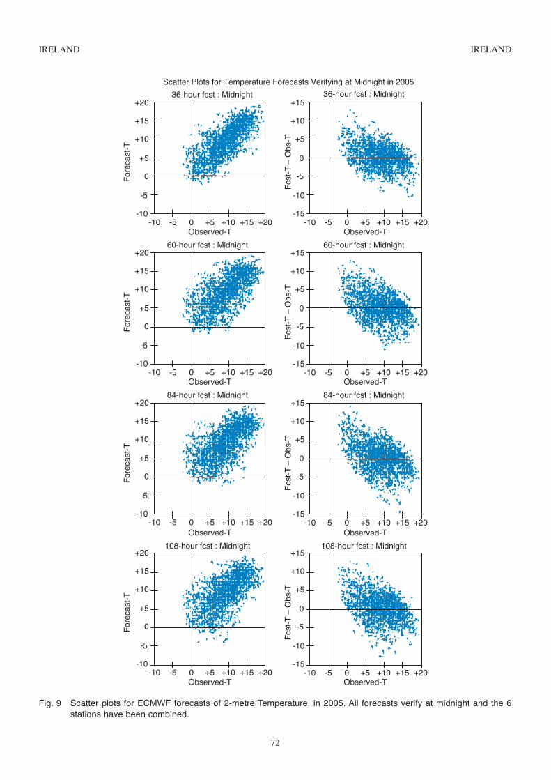
IRELAND IRELAND
72
Fig. 9 Scatter plots for ECMWF forecasts of 2-metre Temperature, in 2005. All forecasts verify at midnight and the 6stations have been combined.
36-hour fcst : Midnight
-10 -5 0 +5 +10 +15 +20Observed-T
-10 -5 0 +5 +10 +15 +20Observed-T
-10
-5
0
+5
+10
+15
+20
For
ecas
t-T
36-hour fcst : Midnight
-15
-10
-5
0
+5
+10
+15
Fcs
t-T
– O
bs-T
Observed-T Observed-T
For
ecas
t-T
Fcs
t-T
– O
bs-T
Observed-T Observed-T
For
ecas
t-T
Fcs
t-T
– O
bs-T
Observed-T Observed-T
For
ecas
t-T
Fcs
t-T
– O
bs-T
60-hour fcst : Midnight60-hour fcst : Midnight
84-hour fcst : Midnight 84-hour fcst : Midnight
108-hour fcst : Midnight108-hour fcst : Midnight
Scatter Plots for Temperature Forecasts Verifying at Midnight in 2005
-10 -5 0 +5 +10 +15 +20-10
-5
0
+5
+10
+15
+20
-10 -5 0 +5 +10 +15 +20-10
-5
0
+5
+10
+15
+20
-10 -5 0 +5 +10 +15 +20-10
-5
0
+5
+10
+15
+20
-10 -5 0 +5 +10 +15 +20-15
-10
-5
0
+5
+10
+15
-10 -5 0 +5 +10 +15 +20-15
-10
-5
0
+5
+10
+15
-10 -5 0 +5 +10 +15 +20-15
-10
-5
0
+5
+10
+15

IRELAND IRELAND
73
Fig. 10 Verification of precipitation forecasts: The plots show smoothed values of the mean monthly Heidke score for 6stations. The smoothing is carried out by means of a 5-month centred running mean. The larger the value of thescore the better the forecast. The results show that there is skill in the rainfall forecast and that the shorter fore-casts are more skilful than the longer.
Smoothed Monthly Scores for Rainfall Forecasts Combined for Six Stations
0.0
0.1
0.2
0.3
0.4
0.5
0.6
0.7
Hei
dke
scor
e
1992 1993 1994 1995 1996 1997 1998 1999 2000 2001 2002 2003 2004 2005
Smoothed Combined Day-1 Rainfall Forecasts for 6 Stations (24-0 hours)
0.0
0.1
0.2
0.3
0.4
0.5
0.6
0.7
Hei
dke
scor
e
1992 1993 1994 1995 1996 1997 1998 1999 2000 2001 2002 2003 2004 2005
Smoothed Combined Day-2 Rainfall Forecasts for 6 Stations (48-24 hours)
0.0
0.1
0.2
0.3
0.4
0.5
0.6
0.7
Hei
dke
scor
e
1992 1993 1994 1995 1996 1997 1998 1999 2000 2001 2002 2003 2004 2005
Smoothed Combined Day-3 Rainfall Forecasts for 6 Stations (72-48 hours)
0.0
0.1
0.2
0.3
0.4
0.5
0.6
0.7
Hei
dke
scor
e
1992 1993 1994 1995 1996 1997 1998 1999 2000 2001 2002 2003 2004 2005
Smoothed Combined Day-4 Rainfall Forecasts for 6 Stations (96-72 hours)

ITALY ITALY
Application and Verification of ECMWF Products in ItalyUfficio Generale per la Meteorologia (UGM) - Centro Nazionale di Meteorologia e ClimatologiaAeronautica (CNMCA by A. Raspanti, A. Galliani
1. Summary of major highlightsIFS deterministic model output from 12Z run (and 00Z run from September 2004) is used at CNMCA as plotted fields in theforecasting department mainly for medium range, also as input to statistical (PPM type) and physical adaptation schemes, andat last as initial and/or boundary conditions for CNMCA Local Area Models (Euro-HRM, HRM, LAMI - non Hydrostatic andEuroLM, non Hydrostatic on European area).Verification of ECMWF products are carried out at CNMCA for operational modelT511 (now T799). Surface parameters and forecast ranges mainly used by weather forecasters are considered.
2. Verification of products
2.1 Objective verification
2.1.1 Direct ECMWF model output
(i) in the free atmosphere
Some basic (MA, MAE or RMSE) verifications for free atmosphere parameters (Vertical profiles interpolated on italian TEMPobservation sites) compared with CNMCA LAMs, are turned out, but not shown on this paper.
(ii) of local weather parameters verified for locations
Objective scores have been computed for ECMWF 12 and 00 utc run (d+1 to d+7) after collecting data, retrieved from 92Italian Synop stations, in several stratifications. Graphical visualizations have been elaborated for a number predictands, herepresented: 2m Temperature, 10m Wind Speed and MSLP (ME, MAE) over Italy and coastal and valley italian stations.
Cumulated precipitations annual event scores (TS, POD/FAR, FBI, KSS) comparing ECMWF and HRM models and quarterlyevent scores respect to fixed thresholds and for d+1 to d+7 ranges are reported.
Data covering the period from Jan-2005 to Dec-2005 have been used for the verification of these parameters and only someselected results are showed in next pages.. Here a short note on results for 12 utc run only.
24 h Cumulated Precipitations: the model shows a good behaviour with respect to seasonal stratification, mainly duringwinter, when precipitation are linked with typical dynamical system and for 10 mm threshold, while for lower and higherthresholds the frequency bias has a worse behaviour.
2m Temperature: good bias, but not very high accuracy is resulted; MAE diurnal excursion, more evident in summer isshowed. The results are more or less independent from range. MAE for valley stations is greater than the coastal one,whilethe mean error is always negative compare to the coastal one, that shows a strange peak also in MAE between October andNovember. In any case slightly greater MAE values occur during summer. The always negative bias for valley stations isprobably due to the difference with the model elevation (no correction done).
10m Wind Speed: light overestimation at 00 and underestimation at 12, except in winter, dynamically driven, where positivebias can be found, but with a worsening accuracy. Always around 2 m/s the value of MAE for almost all the ranges.
(iii) of oceanic waves:
No objective verification is performed, even if the products are daily used and then “verified” form a subjective point of viewby forecasters.
2.1.2 ECMWF model output compared to other NWP models used at CNMCA
ECMWF scores (TS, POD/FAR, FBI, KSS) have been calculated and graphically compared to those evaluated for Italian 12utc run hydrostatic LAM named HRM (d+1, d+2 ranges). They are showed in the next pages on Italian global area and witha morphologic stratification (coastal, valley, mountains).
Better accuracy of ECMWF12 compared with HRM12, that shows an evident and general decreasing of scores for d+2.About the bias, a typical descending rate with thresholds is found with high overestimation for lower thresholds and optimum(fbi=1) close to 12/14 mm/day, after which normal underestimation is evident. Nevertheless, HRM shows a good and betterbias up to 10 mm/day.
74

ITALY ITALY
2.1.3 Post processed products
A statistical adaptation is carried out by a dynamic-statistical model (ARGO), which is a perfect-prog associated to the ECMWF12 utc run. Verification scores for the period from Jan-2005 to Dec-2 005 show little bias improvement escpecially for theearly ranges, but a worsening in accuracy. Better the PPM behaviour for precipitation than for cloudness prediction.
2.1.4 End products delivered to users
Reports are made available quarterly to Intranet users (forecasters, modelists and others).
2.1.5 Seasonal forecasts: planned n the near future
2.2 Subjective verification
2.2.1 Subjective scores: none
2.2.2 Synoptic studies, evaluation of the behaviour of the model (by A. Fuccello)
During last february a Mediterranean Cyclogenesis affected Southern Italy, with strong winds over Sicily, Calabria and Apuliaand significant rainbands over Molise and Campania.
A wide vortex over western Europe (with a cold core over Biscay Gulf) determined a southwestern flow from Morocco toSouthern Italy; it is a case of post-frontal wave and three elements played a crucial role for the event: the transient wave, thejetstreak and the frontal band, as we can see in WV 7.3 picture (in the initial stage there is the leaf shape front, then the darkstrip indicates the stratospheric dry air intrusion).
A good diagnostic tool was the dynamic tropopause, that gave the first signals of the event (an anomaly was formed inMorocco and advected by flow toward the Gabes Gulf ).
The cyclone, moving eastward, affected, as said before, the southern Italian regions, when it was in the cut-off phase, andthe weakening of low was detectable by spiral shape of jetstream, by quite barotropic upper low and bye tropopause anomalyweakening.
75

ITALY ITALY
76
24 h cumulated rainfall February 23
Observed max wind February 23

ITALY ITALY
77
Dynamical Tropopause Height

2.1.2 Seasonal forecasts
Short monthly statements on seasonal forecast trends for Italy are compared to past observations for a preliminary and subjectiveevaluation. Results are under examination, yet.
3. References
ITALY ITALY
78
Translation NOTES on figures Transiente Short Wave Perturbation
Getto Jet or Max Wind
Ciclogenesi Cyclogenesis
Banda nuvolosa frontale Frontal cloud belt
Getto subtropicale Subtropical Jet
Getto Polare Polar Jet

ITALY ITALY
79
Annual Event Scores for Cumulated
Precipitations 2005
POD/FAR -Italy
0
0.5
1
1.5
2
0 0.2 0.5 1 3 6 10 14 18 25 35
Thresholds (mm/day)
FBI - Italy
0
0.5
1
1.5
2
0 0.2 0.5 1 3 6 10 14 18 25 35
Thresholds (mm/day)
TS - Italy
0
0.1
0.2
0.3
0.4
0.5
0 0.2 0.5 1 3 6 10 14 18 25 35
Thresholds (mm/day)
KSS - Italy
0
0.1
0.2
0.3
0.4
0.5
0.6
0.7
0 0.2 0.5 1 3 6 10 14 18 25 35
Thresholds (mm/day)
POD/FAR - valley stations
0.00
0.50
1.00
1.50
2.00
0 0.2 0.5 1 3 6 10 14 18 25 35
Thresholds (mm/day)
FBI - valley stations
0
0.5
1
1.5
2
2.5
0 0.2 0.5 1 3 6 10 14 18 25 35
Thresholds (mm/day)
TS - valley stations
0
0.1
0.2
0.3
0.4
0.5
0.6
0 0.2 0.5 1 3 6 10 14 18 25 35
Thresholds (mm/day)
KSS - valley stations
0
0.1
0.2
0.3
0.4
0.5
0.6
0.7
0 0.2 0.5 1 3 6 10 14 18 25 35
Thresholds (mm/day)
POD/FAR - mountain stations
0.00
0.50
1.00
1.50
2.00
0 0.2 0.5 1 3 6 10 14 18 25 35
Thresholds (mm/day)
FBI - mountain stations
0
0.5
1
1.5
2
2.5
3
3.5
4
0 0.2 0.5 1 3 6 10 14 18 25 35
Thresholds (mm/day)
TS - mountain stations
0
0.05
0.1
0.15
0.2
0.25
0.3
0.35
0.4
0 0.2 0.5 1 3 6 10 14 18 25 35
Thresholds (mm/day)
KSS - mountain stations
0
0.2
0.4
0.6
0.8
1
1.2
0 0.2 0.5 1 3 6 10 14 18 25 35
Thresholds (mm/day)
E12 d+1E12 d+2
H12 d+1H12 d+2

ITALY ITALY
80
Annual Event Scores for Cumulated
Precipitations
Monthly ME and MAE at 00 and 12 UTC from Jan to Dec 2005
POD/FAR -coastal stations
0.00
0.50
1.00
1.50
2.00
0 0.2 0.5 1 3 6 10 14 18 25 35
Thresholds (mm/day)
FBI - coastal stations
0
0.5
1
1.5
2
0 0.2 0.5 1 3 6 10 14 18 25 35
Thresholds (mm/day)
TS - coastal stations
0
0.1
0.2
0.3
0.4
0.5
0 0.2 0.5 1 3 6 10 14 18 25 35
Thresholds (mm/day)
KSS - coastal stations
0
0.1
0.2
0.3
0.4
0.5
0.6
0.7
0 0.2 0.5 1 3 6 10 14 18 25 35
Thresholds (mm/day)
E12 d+1E12 d+2
H12 d+1H12 d+2
2M Temperature - Coastal station 2005
-4.00
-2.00
0.00
2.00
4.00
6.00
8.00
00 12 00 12 00 12 00 12 00 12 00 12 00 12 00 12 00 12 00 12 00 12 00 12
jan feb mar apr may jun jul aug sep oct nov dec
me d+1
me d+2
me d+3
me d+4
me d+5
me d+6
me d+7
mae d+1
mae d+2
mae d+3
mae d+4
mae d+5
mae d+6
mae d+7
Wind Speed (m/s) - Coastal station 2005
-2.00
0.00
2.00
4.00
6.00
00 12 00 12 00 12 00 12 00 12 00 12 00 12 00 12 00 12 00 12 00 12 00 12
jan feb mar apr may jun jul aug sep oct nov dec
me d+1
me d+2
me d+3
me d+4
me d+5
me d+6
me d+7
mae d+1
mae d+2
mae d+3
mae d+4
mae d+5
mae d+6
mae d+7
2M Temperature - Valley station 2005
-4.00
-2.00
0.00
2.00
4.00
6.00
00 12 00 12 00 12 00 12 00 12 00 12 00 12 00 12 00 12 00 12 00 12 00 12
jan feb mar apr may jun jul aug sep oct nov dec
me d+1
me d+2
me d+3
me d+4
me d+5
me d+6
me d+7
mae d+1
mae d+2
mae d+3
mae d+4
mae d+5
mae d+6
mae d+7

ITALY ITALY
81
Monthly ME and MAE at 00 and 12 UTC from Jan to Dec 2005
2M Temperature - Italy 2005
-4.00
-2.00
0.00
2.00
4.00
6.00
00 12 00 12 00 12 00 12 00 12 00 12 00 12 00 12 00 12 00 12 00 12 00 12
jan feb mar apr may jun jul aug sep oct nov dec
me d+1
me d+2
me d+3
me d+4
me d+5
me d+6
me d+7
mae d+1
mae d+2
mae d+3
mae d+4
mae d+5
mae d+6
mae d+7
Wind Speed - Italy 2005
-2.00
0.00
2.00
4.00
00 12 00 12 00 12 00 12 00 12 00 12 00 12 00 12 00 12 00 12 00 12 00 12
jan feb mar apr may jun jul aug sep oct nov dec
me d+1
me d+2
me d+3
me d+4
me d+5
me d+6
me d+7
mae d+1
mae d+2
mae d+3
mae d+4
mae d+5
mae d+6
mae d+7
MSLP - Italy 2005
-4.00
-2.00
0.00
2.00
4.00
6.00
8.00
00 12 00 12 00 12 00 12 00 12 00 12 00 12 00 12 00 12 00 12 00 12 00 12
jan feb mar apr may jun jul aug sep oct nov dec
me d+1
me d+2
me d+3
me d+4
me d+5
me d+6
me d+7
mae d+1
mae d+2
mae d+3
mae d+4
mae d+5
mae d+6
mae d+7
Wind Speed (m/s) -Valley station 2005
-2.00
0.00
2.00
4.00
00 12 00 12 00 12 00 12 00 12 00 12 00 12 00 12 00 12 00 12 00 12 00 12
jan feb mar apr may jun jul aug sep oct nov dec
me d+1
me d+2
me d+3
me d+4
me d+5
me d+6
me d+7
mae d+1
mae d+2
mae d+3
mae d+4
mae d+5
mae d+6
mae d+7

ITALY ITALY
82
Quarterly Event Scores for Cumulated Precipitations
(for fixed threshold) - ITALY 2005
POD/FAR 0,2mm/24hrs
0
0.5
1
1.5
2
2.5
d+1 d+2 d+3 d+4 d+5 d+6 d+7
FBI 0,2mm/24hrs
0.00
0.50
1.00
1.50
2.00
2.50
d+1 d+2 d+3 d+4 d+5 d+6 d+7
1st Quart 2nd Quart
3rd Quart 4th Quart
TS 0,2mm/24hrs
0.00
0.10
0.20
0.30
0.40
0.50
0.60
d+1 d+2 d+3 d+4 d+5 d+6 d+7
KSS 0,2mm/24hrs
0.00
0.20
0.40
0.60
0.80
1.00
d+1 d+2 d+3 d+4 d+5 d+6 d+7
POD/FAR 4 mm/24hrs
0
0.5
1
1.5
2
d+1 d+2 d+3 d+4 d+5 d+6 d+7
FBI 4 mm/24hrs
0.00
0.50
1.00
1.50
2.00
2.50
d+1 d+2 d+3 d+4 d+5 d+6 d+7
TS 4 mm/24hrs
0.00
0.10
0.20
0.30
0.40
0.50
0.60
d+1 d+2 d+3 d+4 d+5 d+6 d+7
KSS 4 mm/24hrs
0.00
0.20
0.40
0.60
0.80
d+1 d+2 d+3 d+4 d+5 d+6 d+7
POD/FAR 10 mm/24hrs
0
0.5
1
1.5
d+1 d+2 d+3 d+4 d+5 d+6 d+7
FBI 10 mm/24hrs
0.00
0.50
1.00
1.50
2.00
2.50
d+1 d+2 d+3 d+4 d+5 d+6 d+7
TS 10 mm/24hrs
0.00
0.10
0.20
0.30
0.40
0.50
d+1 d+2 d+3 d+4 d+5 d+6 d+7
KSS 10 mm/24hrs
0.00
0.10
0.20
0.30
0.40
0.50
0.60
0.70
d+1 d+2 d+3 d+4 d+5 d+6 d+7

ITALY ITALY
83
CLOUD COVERAGE > 5 OCTAVES
QUART. AREA +24 +36 +48 +60 +72 +84 +96 +108 +120 +24 +36 +48 +60 +72 +84 +96 +108 +120
NORTH 0.8 0.7 0.8 0.7 0.8 0.8 0.8 0.7 0.7 0.5 0.5 0.5 0.4 0.5 0.4 0.5 0.4 0.6
CENTRE 0.7 0.6 0.7 0.5 0.7 0.6 0.7 0.5 0.7 0.5 0.3 0.6 0.4 0.5 0.4 0.5 0.4 0.5
SOUTH 0.8 0.6 0.8 0.6 0.7 0.6 0.7 0.6 0.6 0.4 0.2 0.5 0.2 0.4 0.2 0.4 0.2 0.4
NORD 0.7 0.7 0.7 0.7 0.7 0.6 0.6 0.6 0.6 0.4 0.4 0.4 0.4 0.4 0.3 0.4 0.3 0.3
CENTRO 0.8 0.7 0.7 0.7 0.7 0.8 0.7 0.6 0.7 0.4 0.4 0.4 0.4 0.4 0.4 0.4 0.3 0.3
SUD 0.6 0.7 0.7 0.6 0.6 0.6 0.7 0.7 0.6 0.5 0.3 0.3 0.3 0.4 0.3 0.4 0.3 0.4
NORD 0.6 0.3 0.6 0.3 0.5 0.2 0.5 0.1 0.5 0.3 0.2 0.2 0.1 0.2 0.1 0.2 0.1 0.2
CENTRO 0.5 0.0 0.5 0.0 0.8 0.0 0.3 0.0 0.0 0.1 0.0 0.1 0.0 0.1 0.0 0.0 0.0 0.0
SUD 0.5 0.0 0.5 0.0 0.5 0.3 0.5 0.2 0.5 0.1 0.0 0.2 0.0 0.1 0.0 0.1 0.1 0.2
NORD 1.0 0.4 0.9 0.4 0.9 0.4 0.9 0.5 0.9 0.9 0.7 0.9 0.7 0.9 0.7 0.9 0.7 0.9
CENTRO 0.8 0.6 0.8 0.5 0.8 0.5 0.8 0.5 0.9 0.9 0.7 1.0 0.6 0.9 0.7 0.9 0.7 0.9
SUD 0.8 0.6 0.8 0.6 0.8 0.7 0.8 0.6 0.8 1.0 0.5 0.9 0.5 0.9 0.5 0.9 0.5 0.9
MEDIAN ITALY 0.7 0.5 0.7 0.5 0.7 0.5 0.7 0.5 0.6 0.5 0.4 0.5 0.3 0.5 0.3 0.5 0.3 0.5
QUART. AREA +24 +36 +48 +60 +72 +84 +96 +108 +120 +24 +36 +48 +60 +72 +84 +96 +108 +120
NORTH 0.4 0.4 0.5 0.3 0.4 0.4 0.4 0.3 0.4 0.7 0.7 0.6 0.6 0.6 0.6 0.6 0.7 0.8
CENTRE 0.4 0.3 0.4 0.3 0.4 0.3 0.4 0.3 0.4 0.7 0.5 0.7 0.5 0.6 0.5 0.7 0.6 0.7
SOUTH 0.4 0.2 0.4 0.2 0.4 0.2 0.3 0.2 0.3 0.6 0.3 0.6 0.3 0.6 0.3 0.6 0.3 0.6
NORTH 0.3 0.3 0.3 0.3 0.3 0.3 0.3 0.3 0.3 0.5 0.4 0.6 0.4 0.5 0.5 0.5 0.5 0.5
CENTRE 0.3 0.3 0.3 0.3 0.3 0.3 0.3 0.3 0.3 0.5 0.6 0.5 0.7 0.5 0.6 0.5 0.6 0.5
SOUTH 0.4 0.3 0.3 0.2 0.4 0.3 0.3 0.2 0.3 0.7 0.5 0.6 0.5 0.6 0.4 0.6 0.5 0.7
NORD 0.2 0.2 0.2 0.1 0.2 0.1 0.2 0.0 0.1 0.5 0.4 0.4 0.4 0.5 0.4 0.4 0.6 0.3
CENTRO 0.8 0.6 0.8 0.5 0.8 0.5 0.8 0.5 0.9 0.2 0.0 0.2 0.2 0.2 0.4 0.2 0.1 0.2
SUD 0.1 0.0 0.1 0.0 0.1 0.0 0.1 0.1 0.1 0.2 0.1 0.3 0.2 0.3 0.1 0.2 0.3 0.4
NORD 0.8 0.4 0.8 0.4 0.8 0.4 0.8 0.4 0.8 0.9 1.3 1.0 1.4 1.0 1.5 1.1 1.3 1.1
CENTRO 0.8 0.4 0.8 0.4 0.8 0.4 0.8 0.4 0.8 1.1 1.2 1.1 1.2 1.1 1.3 1.1 1.3 1.1
SUD 0.8 0.4 0.7 0.4 0.7 0.4 0.7 0.4 0.7 1.1 0.5 1.1 0.6 1.1 0.6 1.1 0.7 1.1
MEDIAN ITALY 0.5 0.3 0.5 0.3 0.5 0.3 0.4 0.3 0.4 0.6 0.5 0.6 0.6 0.6 0.6 0.6 0.6 0.7
QUART. AREA +24 +36 +48 +60 +72 +84 +96 +108 +120 +24 +36 +48 +60 +72 +84 +96 +108 +120
NORTH 0.6 0.7 0.6 0.7 0.6 0.7 0.6 0.7 0.6 0.3 0.3 0.3 0.3 0.2 0.3 0.3 0.3 0.2
CENTRE 0.6 0.6 0.6 0.6 0.6 0.7 0.6 0.6 0.6 0.2 0.2 0.2 0.2 0.3 0.2 0.2 0.2 0.2
SOUTH 0.6 0.7 0.6 0.7 0.6 0.6 0.6 0.7 0.6 0.2 0.1 0.3 0.1 0.2 0.1 0.2 0.1 0.2
NORTH 0.7 0.8 0.7 0.7 0.7 0.7 0.6 0.7 0.6 0.2 0.3 0.3 0.3 0.2 0.3 0.2 0.2 0.2
CENTRE 0.7 0.8 0.7 0.8 0.7 0.8 0.6 0.8 0.6 0.2 0.3 0.3 0.3 0.2 0.2 0.3 0.2 0.2
SOUTH 0.7 0.8 0.7 0.8 0.7 0.8 0.7 0.8 0.7 0.3 0.3 0.2 0.2 0.3 0.3 0.3 0.2 0.2
NORD 0.7 0.7 0.7 0.7 0.7 0.6 0.6 0.6 0.6 0.4 0.2 0.4 0.4 0.4 0.3 0.4 0.3 0.3
CENTRO 0.8 0.7 0.7 0.7 0.7 0.8 0.7 0.6 0.7 0.4 0.3 0.4 0.4 0.4 0.5 0.4 0.3 0.3
SUD 0.6 0.7 0.7 0.6 0.6 0.6 0.7 0.7 0.6 0.5 0.3 0.3 0.3 0.4 0.4 0.4 0.3 0.4
NORTH 0.8 0.7 0.8 0.7 0.8 0.8 0.8 0.7 0.7 0.3 0.3 0.3 0.3 0.3 0.4 0.3 0.3 0.3
CENTRE 0.7 0.6 0.7 0.5 0.7 0.6 0.7 0.5 0.7 0.3 0.3 0.3 0.3 0.3 0.3 0.3 0.3 0.3
SOUTH 0.8 0.6 0.8 0.6 0.7 0.6 0.7 0.6 0.6 0.4 0.3 0.3 0.2 0.4 0.3 0.3 0.2 0.3
MEDIAN ITALY 0.7 0.7 0.7 0.7 0.7 0.7 0.7 0.7 0.6 0.3 0.3 0.3 0.3 0.3 0.3 0.3 0.2 0.3
THREAT SCORE FREQUENCY BIAS INDEX
III
IV
III
IV
QUARTERLY ARGO VERIFICATIONS 2005 - Perfect Prog of ECMWF 12 utc run
FALSE ALARM RATE PROBABILITY OF DETECTION
I
II
III
IV
I
II
HIT SCORE KSS
I
II

ITALY ITALY
84
QUART. AREA +24 +36 +48 +60 +72 +84 +96 +108 +120 +24 +36 +48 +60 +72 +84 +96 +108 +120
NORTH 0.4 0.6 0.3 0.6 0.2 0.7 0.1 0.7 0.3 0.2 0.2 0.2 0.2 0.3 0.1 0.2 0.2 0.4
CENTER 0.3 0.2 0.3 0.2 0.2 0.2 0.3 0.2 0.2 0.2 0.2 0.3 0.2 0.3 0.1 0.3 0.2 0.3
SOUTH 0.4 0.4 0.4 0.4 0.3 0.3 0.3 0.4 0.4 0.3 0.3 0.3 0.4 0.4 0.3 0.4 0.4 0.3
NORD 0.5 1.0 0.5 1.0 0.4 1.0 0.4 1.0 0.3 0.3 0.1 0.2 0.1 0.2 0.1 0.3 0.2 0.2
CENTRO 0.3 0.2 0.3 0.2 0.3 0.1 0.3 0.2 0.3 0.3 0.2 0.3 0.3 0.3 0.2 0.3 0.2 0.3
SUD 0.3 0.2 0.3 0.2 0.3 0.2 0.3 0.2 0.2 0.3 0.3 0.3 0.2 0.2 0.2 0.3 0.2 0.2
NORTH 0.4 0.7 0.4 0.6 0.5 0.6 0.4 0.7 0.4 0.4 0.2 0.4 0.1 0.5 0.2 0.4 0.2 0.4
CENTER 0.3 0.3 0.4 0.4 0.4 0.3 0.3 0.2 0.4 0.4 0.5 0.4 0.5 0.3 0.4 0.4 0.2 0.3
SOUTH 0.4 0.3 0.5 0.4 0.4 0.3 0.4 0.3 0.5 0.2 0.2 0.2 0.2 0.3 0.2 0.2 0.3 0.2
NORTH 0.4 0.8 0.4 0.7 0.4 0.7 0.4 0.8 0.4 0.5 0.2 0.5 0.2 0.4 0.3 0.4 0.3 0.4
CENTRE 0.3 0.4 0.4 0.5 0.3 0.3 0.3 0.4 0.3 0.3 0.4 0.4 0.3 0.4 0.4 0.3 0.4 0.3
SOUTH 0.4 0.3 0.4 0.3 0.4 0.4 0.4 0.6 0.3 0.4 0.3 0.4 0.3 0.3 0.6 0.3 0.5 0.2
MEDIAN ITALY 0.4 0.5 0.4 0.4 0.4 0.4 0.3 0.5 0.3 0.3 0.3 0.3 0.3 0.3 0.3 0.3 0.3 0.3
QUART. AREA +24 +36 +48 +60 +72 +84 +96 +108 +120 +24 +36 +48 +60 +72 +84 +96 +108 +120
NORTH 0.2 0.2 0.2 0.2 0.2 0.1 0.4 0.2 0.2 1.1 1.4 0.9 1.0 1.0 0.7 0.7 0.7 0.6
CENTER 0.2 0.4 0.2 0.1 0.2 0.1 0.3 0.1 0.1 1.0 0.7 0.9 0.7 0.9 0.7 0.8 0.8 0.9
SOUTH 0.2 0.2 0.2 0.3 0.2 0.2 0.2 0.3 0.2 0.9 1.0 0.8 1.1 1.1 1.0 0.9 1.0 0.9
NORD 0.2 0.1 0.2 0.1 0.1 0.1 0.2 0.1 0.1 1.2 0.8 1.1 0.1 1.0 0.8 0.6 1.1 0.8
CENTRO 0.2 0.3 0.2 0.1 0.2 0.1 0.2 0.1 0.1 0.8 1.1 0.8 1.6 0.9 1.2 0.9 1.0 0.9
SUD 0.1 0.2 0.5 0.2 0.2 0.1 0.4 0.1 0.1 1.5 1.2 1.0 1.3 0.9 1.0 1.1 0.9 1.1
NORTH 0.3 0.2 0.3 0.1 0.3 0.2 0.2 0.2 0.3 1.3 1.0 1.3 0.7 0.5 0.6 0.8 0.6 0.9
CENTER 0.2 0.2 0.3 0.2 0.4 0.2 0.2 0.1 0.2 1.0 1.1 1.0 1.2 1.2 0.9 0.6 0.9 0.7
SOUTH 0.2 0.3 0.2 0.2 0.2 0.2 0.4 0.2 0.2 1.3 0.9 0.9 0.9 0.9 1.0 0.8 1.0 0.8
NORTH 0.3 0.2 0.3 0.2 0.3 0.3 0.3 0.3 0.3 0.9 1.0 0.9 1.0 0.9 0.8 1.0 1.0 1.0
CENTRE 0.2 0.3 0.5 0.2 0.2 0.3 0.2 0.3 0.2 1.0 0.9 1.1 1.0 1.2 1.1 1.0 1.0 0.9
SOUTH 0.2 0.2 0.3 0.2 0.2 0.3 0.4 0.3 0.2 0.8 1.0 0.8 0.7 0.9 0.9 0.9 1.0 0.8
MEDIAN ITALY 0.2 0.2 0.3 0.2 0.2 0.2 0.3 0.2 0.2 1.1 1.0 1.0 0.9 0.9 0.9 0.8 0.9 0.9
QUART. AREA +24 +36 +48 +60 +72 +84 +96 +108 +120 +24 +36 +48 +60 +72 +84 +96 +108 +120
NORTH 0.6 0.4 0.6 0.4 0.6 0.4 0.6 0.4 0.5 0.2 0.1 0.2 -0.2 0.2 0.2 0.1 0.1 0.1
CENTRE 0.6 0.7 0.6 0.7 0.6 0.7 0.6 0.6 0.6 0.1 0.2 0.2 0.3 0.1 0.4 0.0 0.0 0.1
SOUTH 0.6 0.7 0.6 0.7 0.7 0.6 0.6 0.6 0.6 0.1 0.0 0.0 0.0 0.1 0.2 0.1 0.1 0.1
NORTH 0.6 0.3 0.5 0.4 0.6 0.4 0.6 0.3 0.5 0.1 -0.2 0.1 -0.2 0.1 0.2 0.1 -0.1 0.1
CENTRE 0.6 0.7 0.6 0.8 0.6 0.7 0.6 0.6 0.6 0.0 0.1 0.2 0.1 0.2 0.2 0.1 0.1 0.0
SOUTH 0.6 0.5 0.6 0.6 0.6 0.7 0.6 0.7 0.6 0.1 0.0 0.1 0.0 0.1 0.2 0.0 0.2 0.0
NORD 0.7 0.7 0.7 0.7 0.7 0.6 0.6 0.6 0.6 0.4 0.2 0.4 0.4 0.4 0.2 0.4 0.3 0.3
CENTRO 0.8 0.7 0.7 0.7 0.7 0.8 0.7 0.6 0.7 0.4 0.3 0.4 0.4 0.4 0.3 0.4 0.3 0.3
SUD 0.6 0.7 0.7 0.6 0.6 0.6 0.7 0.7 0.6 0.5 0.3 0.3 0.3 0.4 0.3 0.4 0.3 0.4
NORTH 0.8 0.7 0.8 0.7 0.8 0.8 0.8 0.7 0.7 0.3 0.3 0.3 0.3 0.3 0.4 0.3 0.3 0.3
CENTRE 0.7 0.6 0.7 0.5 0.7 0.6 0.7 0.5 0.7 0.3 0.3 0.3 0.3 0.3 0.3 0.3 0.3 0.3
SOUTH 0.8 0.6 0.8 0.6 0.7 0.6 0.7 0.6 0.6 0.4 0.3 0.3 0.2 0.4 0.3 0.3 0.2 0.3
MEDIAN ITALY 0.7 0.6 0.7 0.6 0.7 0.6 0.6 0.6 0.6 0.2 0.2 0.2 0.2 0.2 0.3 0.2 0.2 0.2
FALSE ALARM RATE PROBABILITY OF DETECTION
PRECIPITATIONS > 0 mm/12 h
IV
THREAT SCORE FREQUENCY BIAS INDEX
I
II
I
II
III
III
IV
III
IV
HIT SCORE KSS
I
II

NETHERLANDS NETHERLANDS
Verification of ECMWF products in the Netherlands
1. Summary of major highlightsA 10 day outlook is presented daily on Dutch television showing daytime temperature and precipitation amount includingconfidence bands directly derived from EPS. These broadcasts are provided by Weather News International (WNI), one ofthe Dutch weather service providers.
In cooperation with the Union of Water Boards an automated warning system has been developed aiming at providing optimalmeteorological information in cases of risks of flooding. Large economic losses may arise due to large amounts of precipitationthat exceed the containment capabilities of the Water Board. The critical amount depends, among other things, on the geographyand the pumping capacity of the particular Water Board, the recent precipitation history, but also on the time of year. Dependingon the probability of exceeding this critical precipitation amount (which is different for each of the Water Boards) the watermanager may take precautionary actions. This probability threshold depends on the costs of these measures with respect tothe expected losses that are incurred when no actions would be taken (a so-called cost-loss analysis).
At the moment 13 of the 30 Dutch Water Boards participate in the project. They have specified a number of combinationsof critical precipitation amounts over particular periods and the corresponding probability thresholds. The Water Boards arewarned automatically whenever the predicted probability (obtained from EPS) of exceeding the critical amount is higher thanthe threshold probability.
The warning system covers a 14-day period consisting of a 5-day rainfall history and a 9-day forecast of area averagedprecipitation. Is is operational since december 2003.
2. Verification of products
2.1 Objective Verification
2.1.1 Direct ECMWF model output
(i) in the free atmosphere
The verification of model output based on the objective classification of 500 hPa fields (Kruizinga, 1979) has been continued.This classification (into 27 classes) is performed for 00 UTC fields only. The forecasts are classified for +12, +36, +60 uptoand including +228 lead times. In Table 1 the hit frequencies of forecast classes are presented from 1981 until 2005. Onceagain the last year (2005) proved to be the best year for most forecast times.
2.1.2 ECMWF model output compared to other NWP models
No objective comparative verification has been carried out.
2.1.3 and 2.1.4 post-processed products and end products delivered to users
The MOS interpretation scheme based on ECMWF output products is still operational. In Figs 1 and 2 the skill overclimatology of the MOS scheme for minimum and maximum temperature as well as probability of precipitation is presentedfrom 1984 until 2005 as a time series. Here only the results for station De Bilt are shown.
In Table 2 the skill obtained with the MOS guidance for a few weather elements for De Bilt is presented for the monthsJanuary until November 2005 for day 1 until day 5. The skill of the forecasters is also shown. Note that the verification is onthe same time period but not necessarily on the same cases in this period. For not all days the forecasts of the forecasters wereavailable.
The ECMWF EPS is mainly used to update the medium range forecast and also to assess subjectively the confidence of thedeterministic statements. Moreover, the cluster maps and dispersion information derived from the “plume” of the weatherparameters 2m temperature, 10m wind and precipitation, form the basic input for a 10-day weather outlook. Also a deterministicstatistical guidance for minimum and maximum temperatures is available for which EPS data supply some of the most importantpredictors. An additional MOS based probabilistic system is available in which for a number of thresholds the probability ofexceedance is calculated. This is done for temperature and precipitation for the forecast range day 3 to day 10. Informationfrom EPS as well as information derived from the large scale circulation of the operational model is used. No independentverification results are available at this time.
An objective forecast system for the (conditional) probability of (severe) thunderstorms in the warm half year (mid Aprilto mid October) has been operational in the Netherlands since 2004. Forecasts are given 4 times a day for 12 regions of about90 by 80 km each (see Fig. 3) for 6-hour periods and for projections out to 48 hours in advance. Two predictands are definedfor each region and time period; the first is the probability of a thunderstorm (( 2 lightning discharges) and the second is theconditional probability of a severe thunderstorm (( 500 discharges) under the condition that ( 2 discharges will be detected.
85

NETHERLANDS NETHERLANDS
The predictor set consists of (post-processed) output from both the ECMWF and Hirlam model. Several severe weather indicesare included. An example is given in Fig. 3. In Fig. 4 an objective verification in terms of reliability diagrams is shown forthe summer of 2005. More details are given in Schmeits et al. (2005).
3. References Kruizinga, S. (1979). Objective classification of daily 500 mbar patterns.
Sixth Conference on Probability and Statistics in Atmospheric Sciences, Banff, Alberta, Canada.
Schmeits, M. J., C. J. Kok and D. H. P. Vogelezang (2005). Probabilistic forecasting of (severe) thunderstorms in theNetherlands using model output statistics. Wea. Forecasting, 20, 134-148.
Wilks, D.S. (2005). Statistical methods in the atmospheric sciences: An introduction. Academic Press.
86
Lead time in hours
12 36 60 84 108 132 156 180 204 228
1981 82 64 51 40 27 20
1982 80 66 51 39 29 20
1983 86 72 57 46 33 23
1984 84 69 54 39 28 20
1985 85 72 58 42 28 21
1986 84 72 54 33 29 26
1987 87 72 55 43 30 24
1988 89 79 65 51 35 26
1989 90 81 70 55 45 31
1990 95 80 68 54 40 29 22 14 11 12
1991 93 82 68 52 38 24 17 17 11 10
1992 93 82 68 49 40 27 22 17 13 8
1993 93 83 68 50 37 26 14 12 11 10
1994 91 82 71 50 35 25 20 15 6 7
1995 93 80 71 53 39 30 22 19 13 8
1996 93 80 72 54 42 33 23 16 11 7
1997 94 85 76 53 45 33 26 15 15 14
1998 95 84 70 53 43 32 25 19 14 11
1999 95 85 75 54 46 31 21 12 12 11
2000 96 87 73 65 47 36 26 20 13 10
2001 93 86 74 63 43 34 22 14 11 9
2002 96 88 79 65 50 36 26 21 16 10
2003 96 89 78 66 50 36 26 20 16 10
2004 95 91 80 66 54 38 25 21 14 11
2005 95 90 80 70 56 43 30 21 15 12
Table 1. Relative frequency of hits (%) of ECMWF forecasts for objectively classified flow patterns in the periodsDecember to December ending in 1981, ..., 2005 respectively.
(Hit frequency expected with random forecasts is about 4 %)

NETHERLANDS NETHERLANDS
87
Fig. 1 Skill scores for minimum and maximum temperature for 1984 through 2005. Lead time in days; day 1 is basedon a 36 hours forecast for minimum temperature and +48 for maximum temperature, and so on.
Fig. 2 Skill scores for probability of precipitation for 1984 until 2005. Lead time in days; day 1 is starting at +36 withrespect to the ECMWF model, and so on.
Minimum temperature, skill over climatology
0
10
20
30
40
50
60
70
1984 1986 1988 1990 1992 1994 1996 1998 2000 2002 2004
skill
(%
)
Maximum temperature, skill over climatology
0
10
20
30
40
50
60
70
skill
(%
)
day 1
day 2
day 3
day 5
day 4
day 1
day 2
day 3
day 5
day 4
Probability of precipitation
(18-18), skill over climatology
0
10
20
30
40
50
60
1984
1986
1988
1990
1992
1994
1996
1998
2000
2002
2004
skill
(%
)
day 1
day 2
day 3
day 5
day 4
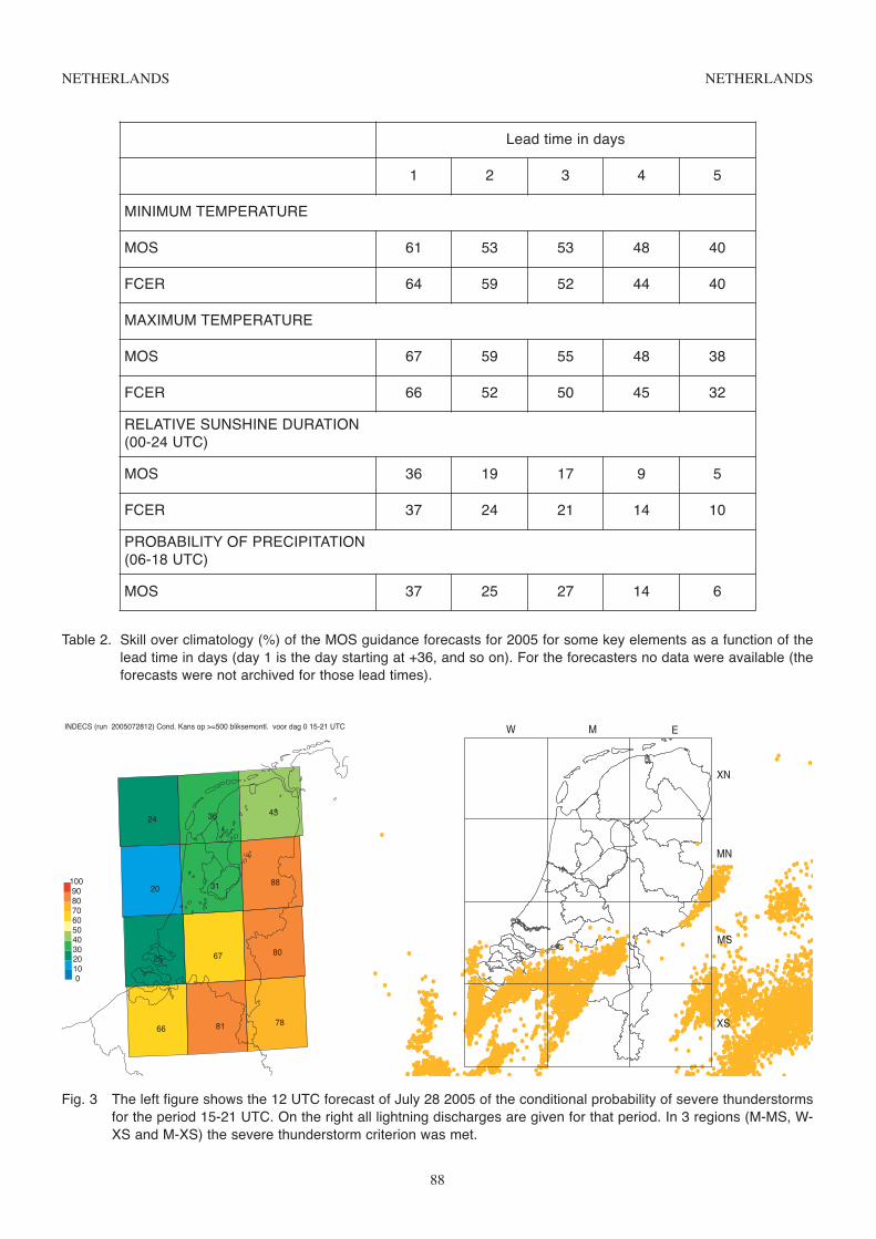
NETHERLANDS NETHERLANDS
88
Lead time in days
1 2 3 4 5
MINIMUM TEMPERATURE
MOS 61 53 53 48 40
FCER 64 59 52 44 40
MAXIMUM TEMPERATURE
MOS 67 59 55 48 38
FCER 66 52 50 45 32
RELATIVE SUNSHINE DURATION (00-24 UTC)
MOS 36 19 17 9 5
FCER 37 24 21 14 10
PROBABILITY OF PRECIPITATION(06-18 UTC)
MOS 37 25 27 14 6
Table 2. Skill over climatology (%) of the MOS guidance forecasts for 2005 for some key elements as a function of thelead time in days (day 1 is the day starting at +36, and so on). For the forecasters no data were available (theforecasts were not archived for those lead times).
Fig. 3 The left figure shows the 12 UTC forecast of July 28 2005 of the conditional probability of severe thunderstormsfor the period 15-21 UTC. On the right all lightning discharges are given for that period. In 3 regions (M-MS, W-XS and M-XS) the severe thunderstorm criterion was met.
INDECS (run 2005072812) Cond. Kans op >=500 bliksemontl. voor dag 0 15-21 UTC
66 81 78
25 67 80
20 31 88
24 36 43
0 10 20 30 40 50 60 70 80 90
100

NETHERLANDS NETHERLANDS
Fig. 4 Reliability diagrams of (a) +6 h forecasts for all 12 pooled regions, (b) +12 h forecasts for the 6 pooled landregions, (c) +12 h forecasts for the 6 pooled coastal regions, (d) +18 h forecasts for the 6 pooled land regions,(e) +18 h forecasts for the 6 pooled coastal regions, and (f) +24 h forecasts for all 12 pooled regions, as com-puted by the 00 UTC run of the MOS severe thunderstorm forecast system. The verification period is from 16April - 15 October 2005. In these diagrams the observed frequencies of severe thunderstorm occurrence areshown, conditional on each of the 10 possible forecast probabilities (indicated by diamonds). For perfectly reli-able forecasts these paired quantities are equal, yielding all points in the diagram falling on the diagonal line. Thedotted line indicates the 2000-2004 climatology and the dashed line the sample climatology. The dash-dotted lineindicates the “no skill” line. The histogram on the right portrays the relative frequency of use of the forecasts. HereBS is short for Brier score, BSS for Brier skill score, UNC for uncertainty, REL for reliability and RES for resolu-tion (Wilks, 2005), and N is the total number of cases.
89
a)
b) c)
e) f)
d)

NORWAY NORWAY
Verification of ECMWF products in Norway
1. Summary of major highlightsThe ECMWF products are widely used by forecasters to make forecasts for the public, as boundary values in HIRLAM, asbasis for LAM ensembles, as input to statistical methods, and more or less directly by customers. The forecasts are mainlyverified directly against observations and less against computed area observations. Results are presented in quarterly reportsand on internal web pages.
2. Verification of products
2.1 Objective verification
2.1.1 Direct ECMWF model output
(i) in the free atmosphere.
(ii) of local weather parameters.
Local weather parameters are continuously verified against a large number of observations. An example for 2 metre temperatureis given in figure 1 with quarterly mean errors (ME) and standard deviations of errors (SDE) for all Norwegian synoptic stationsfor the autumn 2005. The results show large geographical variations, but in general the ME can mostly be explained by thedifferences in elevations.
Figure 2 demonstrates the quality of the precipitation forecasts at synoptic stations for the autumn 2005. In general, verylarge amounts are underestimated and small amounts seem to occur too often, at least when compared to rain gaugemeasurements. Overestimation is also present just east of the mountains in the south of Norway where the climate is drycompared to the western part.
(iii) of oceanic waves.
2.1.2 ECMWF model output compared to other NWP models
An example of 10 metre wind speed forecasts from ECMWF compared to HIRLAM10, HIRLAM20 and UM4 is given infigures 3 and 4, with time series of ME and SDE from December 2003 to February 2006. The results are averaged over variousselections of stations. Most noticeable is the systematic underestimation along the coastline and in the mountainous regions.The main contribution to the negative bias is the lack of strong winds in the model at these sites.
Precipitation forecasts are verified by means of several measures in addition to ME, SDE and MAE. Figure 5 shows HitRate, False Alarm Rate, False Alarm Ratio, Equitable Threat Score and Hanssen-Kuipers Skill Score as a function of exceedingthreshold for the autumn 2005 for ECMWF, HIRLAM20, HIRLAM10 and UM4. For this season, dominated by frontalprecipitation systems, ECMWF and UM4 had in general better scores than HIRLAM20/10.
2.1.3 Post-processed products
Probabilistic forecasts in terms of quantiles for maximum wind speed, 2 metre temperature and daily precipitation have beengenerated operationally since autumn 2003. The forecasts are produced by local quantile regression and based on daily ECMWFforecasts (12 UTC) and about 3 years of historical data. At the time of writing there are no summarising results available, butit has been noticed that the distributions (quantiles) sometimes are not smooth enough for “extreme” events.
A Kalman filter procedure is operationally applied to 2 metre temperature forecasts. The quality of 2 metre temperatureforecasts, direct model output and Kalman filter corrected, are evaluated by ME, SDE and mean absolute errors (MAE)presented as a function of forecast lead time. In figure 6 the results for 2005 averaged over 170 stations are presented; theKalman filter removes the biases (at least for the shortest lead times which it is designed to do), but the SDE remains moreor less unchanged.
2.1.4 End products
2.1.5 Seasonal forecasts
Seasonal temperature forecasts are presented on external web pages for an area covering the Nordic countries, Iceland andGreat Britain. The quality of the seasonal temperature forecasts is evaluated by comparing them to observations at a selectionof Norwegian cities. Results for Oslo are shown as an example in figure 7. The correlation between the ensemble mean andthe observed temperature is 0.61 for Oslo for this time period.
90

NORWAY NORWAY
2.2 Subjective verification
2.2.1 Subjective scores
The duty forecasters carry out subjective verification of some of the available numerical products. A few scores are dailycalculated by looking at the position and strength of the most significant low or high in the forecast area and the position ofthe fronts associated with these systems. The studies conclude that the model of ECMWF still is the best.
2.2.2 Synoptic studies, evaluation of the behaviour of the model
2.2.3 Seasonal forecasts
ReferencesAndersen, J.M.: Prognoseverifikasjon for året 2005. Internal web document (in Norwegian).
Bremnes, J.B., and Homleid, M.: Verification of operational numerical weather prediction models December 2004 to February2005. met.no note, no. 11/2005
Bremnes, J.B., and Homleid, M.: Verification of operational numerical weather prediction models March to May 2005. met.nonote, no. 28/2005
Bremnes, J.B., and Homleid, M.: Verification of operational numerical weather prediction models June to August 2005. met.nonote, no. 29/2005
Bremnes, J.B., and Homleid, M.: Verification of operational numerical weather prediction models September to November2005. met.no note, no. 1/2006.
91

NORWAY NORWAY
92
ME EC 12+48
−0.3−1.8
−1.7
−1.6
−1
−1.6−2.5
−0.6
−2.2
−1.9
−0.1
−2.1
−0.4
−1.4
−1.9
−0.6
−0.9
−0.5
−0.5−1.1
0
−0.8
−1.2
−0.5
−0.7
−3.9
−2
0.2
−1.3 −0.8−0.4
−1.2 −2.6
SDE EC 12+48
1.31.1
2.7
1.3
1.1
2.91.5
2.6
2.1
1.4
2.6
1.9
3.2
2.3
1.3
1.7
1.1
0.8
0.91.4
0.9
1.8
1.1
1
1.4
2.6
1.2
2.3
2.1 1.81
1.5 2.4
−0.30.9
−0.7
−1.5
−2.7
−0.8
−0.5
1.1
−0.1
−1.2
−0.8
−1.4
0.3
−1.3
−0.3
−1.2
−1.1
−0.8
−1.2
−0.9
−0.2
−0.2
−0.4
−0.9
−0.2
−1
−0.4
−0.1
0.1
−1.6−1.5
−4.1
−1.2
−0.4
−1.2
−1.1−0.4
−2.3
−2.2
−2.6
−0.2
−1
−0.8−2.4
−1.7
−2.6
−1.3
−0.3
−1.5
−6.7
−0.4
−1.4
−1.9
−1.8
−1.9
−2.5
−1.3
2.81.4
2.8
1.8
2.6
1.7
1.9
1.5
1.9
2.4
1.6
0.9
1.8
1
1.4
1.9
1
2.2
1.4
1.8
2.1
1.2
1.3
2.1
1
1.5
1.4
1.8
1.3
11.4
3.1
2.3
1
1.5
1.71.6
2.4
1.9
2.4
1.8
1
1.41.4
1.7
2.4
2.8
1.6
1.7
3.6
0.8
1.2
1.5
1.5
1.7
2.1
1.7
T2m
01.09.2005 − 30.11.2005
Fig. 1 Mean errors (left) and standard deviation of errors (right) of ECMWF 12+48 temperature (2m) forecasts.

NORWAY NORWAY
93
ME EC 12+42
−0.32.1
−0.7
0
01.8
0.3
1.4
0.7
−4
1.1
0.10.7
2.41.2
1.8
1
0.1
−2.3
5
−0.9
0.1
−1.2 0.3−0.8
0.5 1
SDE EC 12+42
5.24.4
4
4
8.42.6
2.1
2.3
2.3
20.2
1.7
22.4
4.53.9
4.4
3
4.4
8.2
4.3
6.8
2.1
3.9 212.5
3.2 3.5
31.9
2.6
2
0.6
1.5
1
0.9
−0.1
0.6
1.4
2.8
0.7
2.1
−0.9
0.8
1.5
0.5
0.6
−0.1
0
0.8 0.1
−0.1
0.1
−0.7
1.3
0.9
2.4
0.2
0.5
−0.8
0.5
1.71.1
0.8
0.7
1
0.4−2.2
−6
1.2
−1.9
−1.8
0.8
3.3
3.3
3.6
−0.4
3.6
−0.5
−1.7
3.42.6
5.3
4.7
2.5
2.9
2.3
2.6
3.2
2.9
2.6
6.1
5.8
5.1
5.6
3.5
3.6
4.9
2.8
3.9
3.5
2.7 3.1
2.4
2.9
4
2.8
4.9
6.3
4.1
2.9
12.5
3.2
2.83.3
2.8
2.5
3.5
8.810.2
14
6.3
10.1
8.1
7.4
6.4
7.5
9.3
7
7.8
10.2
8.5
RR24
01.09.2005 − 30.11.2005
Fig. 2 Mean errors (left) and standard deviation of errors (right) of ECMWF 12+42 daily accumulated precipitation forecasts.

NORWAY NORWAY
94
Dec03 Feb04 Apr04 Jun04 Aug04 Oct04 Dec04 Feb05 Apr05 Jun05 Aug05 Oct05 Dec05 Feb06
−1.0
−0.5
0.0
0.5
1.0
180 Norwegian stations
UM4 Hirlam10 Hirlam20 ECMWF
12+18,+30 UTC
Dec03 Feb04 Apr04 Jun04 Aug04 Oct04 Dec04 Feb05 Apr05 Jun05 Aug05 Oct05 Dec05 Feb06
−1.0
−0.5
0.0
0.5
1.0
127 EWGLAM stations
Dec03 Feb04 Apr04 Jun04 Aug04 Oct04 Dec04 Feb05 Apr05 Jun05 Aug05 Oct05 Dec05 Feb06
−3
−2
−1
0
1
43 Norwegian coastal stations
Dec03 Feb04 Apr04 Jun04 Aug04 Oct04 Dec04 Feb05 Apr05 Jun05 Aug05 Oct05 Dec05 Feb06
−3
−2
−1
0
1
5 Norwegian mountainous stations
Mean Error of wind speed
Fig. 3 Monthly mean errors from December 2003 to February 2006 of ECMWF, HIRLAM10, HIRLAM20 and UM412+18,+24,+36,+48 wind speed forecasts.

NORWAY NORWAY
95
Dec03 Feb04 Apr04 Jun04 Aug04 Oct04 Dec04 Feb05 Apr05 Jun05 Aug05 Oct05 Dec05 Feb06
1.0
1.5
2.0
2.5
3.0
3.5
180 Norwegian stations
UM4 Hirlam10 Hirlam20 ECMWF
12+18,+30 UTC
Dec03 Feb04 Apr04 Jun04 Aug04 Oct04 Dec04 Feb05 Apr05 Jun05 Aug05 Oct05 Dec05 Feb06
1.0
1.5
2.0
2.5
3.0
3.5
127 EWGLAM stations
Dec03 Feb04 Apr04 Jun04 Aug04 Oct04 Dec04 Feb05 Apr05 Jun05 Aug05 Oct05 Dec05 Feb06
1.0
1.5
2.0
2.5
3.0
3.5
43 Norwegian coastal stations
Dec03 Feb04 Apr04 Jun04 Aug04 Oct04 Dec04 Feb05 Apr05 Jun05 Aug05 Oct05 Dec05 Feb06
1.0
1.5
2.0
2.5
3.0
3.5
5 Norwegian mountainous stations
Standard Deviation of Error of wind speed
Fig. 4 Monthly standard deviation of errors from December 2003 to February 2006 of ECMWF, HIRLAM10, HIRLAM20and UM4 12+18,+24,+36,+48 wind speed forecasts.
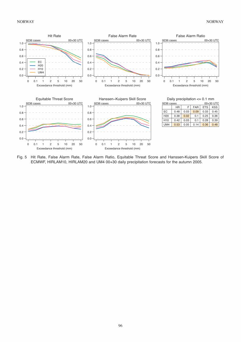
NORWAY NORWAY
96
Exceedance threshold (mm)
0.0
0.2
0.4
0.6
0.8
1.0
0 0.1 1 2 5 10 20 50
Hit Rate9236 cases 00+30 UTC
ECH20H10UM4
Exceedance threshold (mm)
0.0
0.2
0.4
0.6
0.8
1.0
0 0.1 1 2 5 10 20 50
False Alarm Rate9236 cases 00+30 UTC
Exceedance threshold (mm)
0.0
0.2
0.4
0.6
0.8
1.0
0 0.1 1 2 5 10 20 50
False Alarm Ratio9236 cases 00+30 UTC
Exceedance threshold (mm)
0.0
0.2
0.4
0.6
0.8
1.0
0 0.1 1 2 5 10 20 50
Equitable Threat Score9236 cases 00+30 UTC
Exceedance threshold (mm)
0.0
0.2
0.4
0.6
0.8
1.0
0 0.1 1 2 5 10 20 50
Hanssen−Kuipers Skill Score9236 cases 00+30 UTC
Daily precipitation <= 0.1 mm9236 cases 00+30 UTC
HR F FAR ETS KSS
EC
H20
H10
UM4 0.53 0.05 0.14 0.36 0.48
0.42 0.03 0.1 0.28 0.39
0.38 0.02 0.1 0.25 0.36
0.48 0.03 0.09 0.33 0.45
Fig. 5 Hit Rate, False Alarm Rate, False Alarm Ratio, Equitable Threat Score and Hanssen-Kuipers Skill Score ofECMWF, HIRLAM10, HIRLAM20 and UM4 00+30 daily precipitation forecasts for the autumn 2005.

NORWAY NORWAY
97
0
1
2
3
MA
E (
°C
)
Temperature 01.01.2005 − 31.12.2005
0
1
2
3
4
SD
E (
°C
)
ECMWF12 ECMWF12*K
+6 +24 +42 +60 +78 +96 +114 +132 +150 +168 +186 +204 +222 +240
−1.5
−1.0
−0.5
0.0
Forecast length
ME
( °
C )
Fig. 6 ME, SDE and MAE as a function of forecast lead time for 2 metre temperature forecasts by ECMWF with andwithout a Kalman filter. The scores are averaged over 170 synoptic stations.

NORWAY NORWAY
98
Fig. 7 Seasonal forecasted and observed 2 metre temperature from February 2002 to summer 2006 for Oslo. Theensemble means are marked with a grey “ball”, the observed mean temperature with a red “ball” and the ensem-ble members with small dots.

PORTUGAL PORTUGAL
99
Verification of ECMWF Products at Meteorological Institute, Portugal
1. Summary of major highlightsThe medium-range weather forecasts in Portugal are mainly based on the ECMWF deterministic forecasts. The ECMWF directmodel output forecasts are interpolated and verified against the data from 68 meteorological stations. The main results obtainedfrom some statistical measures are presented here, for the period from January 2005 to December 2005.
2. Application of products
2.1 Post-processing of deterministic model output
• Thermal frontal parameter and Q vector convergence
• Temperature advection at 850hPa and vorticity advection at 500hPa
• Low-level moisture convergence
• Total-Totals and Jefferson indices.
3. Verification of products
3.1 Objective verification
3.1.1 Direct ECMWF model output.
Figures 1 to 6 show the RMSE and bias of 2m temperature (T2m), 2m relative humidity (RH2m) and 10m wind speed (V10m),for autumn and spring seasons. A cold bias is visible in most of the stations, except near Serra da Estrela mountain (bias >3ºC). Moreover, the model tends to overestimate V10m, except in mountainous regions. It is also visible that the smallesterrors of V10m occur in inland southern region.
The RMSE of T2m over Portugal as function of forecast range and seasons is shown in figure 7. It is clear that the largesterrors occur in summer. Moreover, the model tends to underestimate T2m at 12 UTC, while a warm bias is visible at 00 UTC(figure 8). The results also show that the model slightly overestimates (figure 10). In addition, there is a tendency to overestimatethe wind speed, mainly at 00 UTC (figure 12).

PORTUGAL PORTUGAL
100
Fig. 1 Spatial distribution of 2m temperature RMSE over Portugal, for H+24 (valid at 12 UTC), for fall (left) and spring(right) seasons. RMSE values smaller than 1.6ºC are in green. Values between 1.6 and 3ºC are in blue and val-ues larger than 3ºC are in red.
Fig. 2 Spatial distribution of 2m temperature bias over Portugal, for H+24 (valid at 12 UTC), for fall (left) and spring(right) seasons. Positive values are in red (> 1.5ºC) and orange (≤ 1.5ºC). Negative values are in blue (< -1.5ºC)and cyan (≥-1.5ºC).

PORTUGAL PORTUGAL
101
Fig. 3 Spatial distribution of 2m relative humidity RMSE over Portugal, for H+24 (valid at 12 UTC), for fall (left) andspring (right) seasons. RMSE values smaller or equal than 10% are in green. Values between 10.1 and 15% arein blue. Values larger than 15% are in red.
Fig. 4 Spatial distribution of 2m relative humidity bias over Portugal, for H+24 (valid at 12 UTC), for fall (left) and spring(right) seasons. Positive values are in red (≥ 10%) and orange (< 10%). Negative values are in blue (< -10%) andcyan (≥-10%).

PORTUGAL PORTUGAL
102
Fig. 5 Spatial distribution of 10m wind speed RMSE over Portugal, for H+24 (valid at 12 UTC), for fall (left) and spring(right) seasons. RMSE values smaller than 1.5m s-1 are in green. Values between 1.5 and 3 m s-1 are in blueand values larger than 3 m s-1 are in red.
Fig. 6 Spatial distribution of 10m wind speed bias over Portugal, for H+24 (valid at 12 UTC), for fall (left) and spring(right) seasons. Positive values are in red (≥ 1.5m s-1) and orange (< 1.5m s-1). Negative values are in blue (<-1.5m s-1) and cyan (≥ -1.5m s-1).

PORTUGAL PORTUGAL
Fig. 7 RMSE of 2m temperature over Portugal as function of forecast range, for summer, spring, fall and winter sea-sons for 12 UTC.
103
Fig. 9 RMSE of 2m relative humidity over Portugal as function of forecast range, for summer, spring, fall and winter sea-sons for 12 UTC.
Fig. 8 Bias of 2m temperature over Portugal as function of forecast range, for summer, spring, fall and winter seasonsfor 12 UTC (left) and for 00 UTC (right).

PORTUGAL PORTUGAL
104
Fig. 11 RMSE of 10m wind speed over Portugal as function of forecast range, for summer, spring, fall and winter sea-sons for 12 UTC.
Fig. 10 Bias of 2m relative humidity over Portugal as function of forecast range, for summer, spring, fall and winter sea-sons for 12 UTC (left) and for 00 UTC (right).
Fig. 12 Bias of 10m wind speed over Portugal as function of forecast range, for summer, spring, fall and winter seasonsfor 12 UTC (left) and for 00 UTC (right).
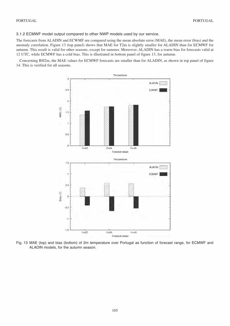
PORTUGAL PORTUGAL
3.1.2 ECMWF model output compared to other NWP models used by our service.
The forecasts from ALADIN and ECWMF are compared using the mean absolute error (MAE), the mean error (bias) and theanomaly correlation. Figure 13 (top panel) shows that MAE for T2m is slightly smaller for ALADIN than for ECMWF forautumn. This result is valid for other seasons, except for summer. Moreover, ALADIN has a warm bias for forecasts valid at12 UTC, while ECMWF has a cold bias. This is illustrated in bottom panel of figure 13, for autumn.
Concerning RH2m, the MAE values for ECMWF forecasts are smaller than for ALADIN, as shown in top panel of figure14. This is verified for all seasons.
105
Fig. 13 MAE (top) and bias (bottom) of 2m temperature over Portugal as function of forecast range, for ECMWF andALADIN models, for the autumn season.

PORTUGAL PORTUGAL
106
Fig. 15 MAE (top) and bias (bottom) of 2m relative humidity over Portugal as function of forecast range, for ECMWF andALADIN models, for the autumn season.
Fig. 14 Anomaly correlation of 2m temperature over Portugal as function of forecast range, for ECMWF and ALADINmodels, for the autumn season.

ROMANIA ROMANIA
107
Verification of ECMWF products in RomaniaThe National Meteorological Administration (NMA)
1. Summary of major highlights of use and verification.(i) A major change in improving the forecast quality by Bucharest National Weather Forecasting Centre (NWFC) was madelast year since we are using all ECMWF products that have been made available for the member state users on the ECMWFweb site.
NWFC and also the Romanian Regional Weather Forecasting Centres used the products from both deterministic and ensembleECMWF forecasts (daily for short and medium range forecast with good results), usually in conjunction with the outputs ofhigh-resolution limited-area models ALADIN and LM (for short range) and ARPEGE and DWD (for medium range).
During the year 2005 we had to focus on improving the quantitative precipitation forecasts.
Following the encouraging predictability results of the ECMWF model within the period 13-19 April 2005 (when heavyrainfalls occurred in Romania, causing the most damaging severe flooding since 1975 especially in the south-western part)NWFC has started using operationally the EPS products for the medium-range forecast, especially in cases of extreme weatherevents. At the beginning, forecasters used the deterministic model fields (TA500, T850, T500, MSLP and wind at 700 and500 hPa, Relative Humidity, 2m temperature), then the Ensemble Prediction System that allowed us to make a probabilisticapproach in order to develop capability to estimate the uncertainty of the forecasts. The EPS forecasts for most of the caseshad high skill scores for anticipations up to 7 days and even for 10 days. At the met-ops room forecasters use the ClusterAnalysis, the probabilities maps for different parameters (in particular 24h cumulated precipitation, precipitation rateprobability, 10m wind gust probabilities) and thresholds. In order to evaluate the occurrence of weather events a very usefultool is the EFI maps for parameters directly related to severe weather. Being a measure of the distance from the climate to theforecast distribution the EFI helps us to estimate the rainfall amount. Forecasters use the EPSgrams for the region which wasindicated as the most likely to be affected by intense precipitation.
In order to extend the weather forecast for Romania beyond the 10 days range, since January 2005 the MFS products fromECMWF web site are being used. That means a permanent testing of the weekly forecasting products and adapting them forRomania. The main MFS products analyzed once a week are as follows:
– weekly ensemble mean anomaly maps for 2m temperature, total precipitation, MSLP and 500 hPa geopotential;
– probability that the same parameters be at least 10 % different from the weekly means;
– tercile probability maps for 2m temperature and total precipitation.
By analyzing all the information provided by MFS products, maps for Romania have been made, including two very importantparameters with respect to their superior and inferior terciles: the average weekly temperature and total precipitation.
(ii) The MOS system was developed in 2004 and the results are used in the operational activity. A verification system of theMOS forecasts was built in 2005 and the monthly results are available on the Intranet web-site.
At the end of every month, seasonal forecast charts from the ECMWF are analyzed as consultative material added to theresults of the statistical models used in NMA to issue the 3-month forecast for Romania.
2. Verification of products.
2.1 Objective verification
2.1.1 Direct ECMWF model output (both deterministic and EPS)
In 2005 we started working on a verification procedure for the deterministic model (DMO), using observations from 160synoptic stations. The following parameters are being verified:
• sea level pressure
• 2m temperature
• wind speed
• total cloudiness, by 3 categories
Procedures are being implemented for the verification of extreme temperatures, wind direction and precipitation.
Scores are computed corresponding to the ones recommended in the ECMWF “Tehnical memorandum No. 430”. Some ofthe graphs are attached in the annex of this report.

ROMANIA ROMANIA
The used interpolation method is “the nearest grid point to the synoptic station”, the verification procedures being computedmonthly and seasonally for every synoptic station and averaged over the whole analysis domain.
The verification results are presented in comparison with the MOS system. The reference forecast used to calculate the SkillScore for both DMO and MOS is “persistency”.
2.1.2 ECMWF model output compared to other NWP models used by NMA
NMA continued the comparative verification of MOS-ECMWF with the other systems: MOS-ALADIN and MOS-ARPEGE,for the extreme temperatures forecasts, at 10 synoptic stations.
2.1.3 Post -processed products
For MOS-ECMWF, verification procedures were performed on a regular basis for the following parameters: 2m temperature,extreme temperatures, total cloudiness, 6h cumulated precipitation and 10m wind (speed and direction). The scores werecomputed taking into account all 160 Romania synoptic stations. Existing verification procedures were extended by computingmore significant scores. All the verification scores are available on the intranet website.
As an example, the scores of the verification of MOS-ECMWF forecast are briefly discussed:
a) 2m temperature - TS
As one can notice in Fig.1-Fig.4 the MOS reduces the model’s BIAS, less in the winter season, where MOS has a positivebias to the numerical model. The explanation stands in the lack of information on the soil surface state from the statisticalmodel. The contribution brought by the statistical model is about 20 C in RMSE terms. The best corrections that MOS bringsare noticed in the hill and mountain area.
b) Mean Sea Level Pressure - MSL
A small negative BIAS is noticed in almost all the seasons in the range of 1mb, less in the spring season. RMSE has valuesunder 5 mb with the 120 hours anticipation. The best forecasts were achieved during the autumn and spring season respectively.The summer of 2005, even though RMSE has low values, the Skill Score and RV indicate a lower score forecast than the onecorresponding to the other two seasons (Fig.5 and Fig.6).
c) Total Cloudiness - TCC
To perform a comparison of the two models’ performance, the verification was made for three categories, corresponding tothe statistical model (Multiclass Discriminant Analysis).
There are differences from a season to season regarding the quality of the two models, the “added value” by the MOS beingabout 5-10% in PC terms.
Both models have low performance for the second class “Partly cloudy” (POD - low and FAR - high values). The extremeclasses - first class “No clouds” and the third one “Cloudy” are better forecasted, but there are also differences from oneanticipation to another and from a season to another season.
In the spring of 2005 (Fig.7), MOS was superior to the DMO for the “Cloudy” class (POD-high, FAR less than the DM andCSI higher values). For the “No Clouds” class, both models had similar performances. In the summer (Fig.8) however, theatmospheric instability being higher, the convective cloudiness more enhanced, the scores obtained for the first and secondclass have a strong diurnal cycle: low scores corresponding to the day-time (+24h, +48h, etc) and higher scores correspondingto the night-time. There are no notable differences for both models’ performance regarding those two classes. Forecasts forthe third class of cloudiness are lower than the preceding season, but here MOS seems to work better than DMO.
In autumn (Fig.9), the first and third class have similar POD scores, but FAR has higher scores for the first class. The diurnalcycle in the scores evolution maintains the same for the first and second class. In the winter of 2005-2006 (Fig.10), the diurnalcycle in the scores evolution decreases, MOS maintaining the superiority over the DMO for the third class.
Therefore, MOS is superior to DMO in all the seasons concerning the third class of cloudiness. The second class has thelowest forecasts; MOS does not bring an important “added value” to DMO.
The first class “No clouds” is better forecasted than the second one, the “added value” of MOS being related to the day-time moment and seasons.
d) 10 m wind speed
The wind speed is a parameter well forecasted by DMO, and the correction brought by MOS is about 1-2 m/s (in RMSE terms).DMO has a negative bias, compared to MOS which brings the bias to zero (Fig.11-Fig.14).
2.1.4 End products delivered to users
2.1.5 Seasonal forecasts
108

ROMANIA ROMANIA
2.2 Subjective verification
2.2.1 Subjective scores
2.2.2 Synoptic studies, evaluation of behavior of the models
The synoptic case studies have shown better accuracy of the ECMWF model parameters for both the 00 and 12 UTC runs.Occasionally the blocking circulation over Eastern Europe was underestimated, but the model showed a clear improvementin precipitation forecast (with occasional slight overestimation of light rain events).
2.2.3 Seasonal forecasts
The skill of seasonal forecasts from the ECMWF for the Romania continues to be rather low.
3. References
109
Fig. 1 Mean error (BIAS) and Root mean square error (RMSE) for 2m temperature (upper panel) and VarianceReduction and MSE_SS (lower panel), averaged over 168 stations. Spring 2005. (Red: DMO, Blue: MOS).

ROMANIA ROMANIA
110
Fig. 2 Mean error (BIAS) and Root mean square error (RMSE) for 2m temperature (upper panel) and VarianceReduction and MSE_SS (lower panel), averaged over 168 stations. Summer 2005. (Red: DMO, Blue: MOS).
Fig. 3 Mean error (BIAS) and Root mean square error (RMSE) for 2m temperature (upper panel) and VarianceReduction and MSE_SS (lower panel), averaged over 168 stations. Autumn 2005. (Red: DMO, Blue: MOS).

ROMANIA ROMANIA
111
Fig. 4 Mean error (BIAS) and Root mean square error (RMSE) for 2m temperature (upper panel) and VarianceReduction and MSE_SS (lower panel), averaged over 168 stations. Winter 2005. (Red: DMO, Blue: MOS).
Fig. 5 Mean error (BIAS) and Root mean square error (RMSE) for Mean Sea Level Pressure (MSL) (upper panel) andVariance Reduction and MSE_SS (lower panel), averaged over 168 stations. Winter 2004 and Winter 2005. (Red:2004, Blue: 2005).

ROMANIA ROMANIA
112
Fig. 6 Mean error (BIAS) and Root mean square error (RMSE) for Mean Sea Level Pressure (MSL) (upper panel) andVariance Reduction and MSE_SS (lower panel), averaged over 168 stations. Spring - Autumn 2005. (Red:Spring, Blue: Summer, Green: Autumn).
Fig. 7 Scores for total cloudiness (TCC), averaged over 168 stations, DMO versus MOS - Spring 2005.

ROMANIA ROMANIA
113
Fig. 8 Scores for total cloudiness (TCC), averaged over 168 stations, DMO versus MOS - Summer 2005.
Fig. 9 Scores for total cloudiness (TCC), averaged over 168 stations, DMO versus MOS - Autumn 2005.

ROMANIA ROMANIA
114
Fig. 10 Scores for total cloudiness (TCC), averaged over 168 stations, DMO versus MOS - Winter 2005.
Fig. 11 Mean error (BIAS) and Root mean square error (RMSE) for Wind Speed (FF) (upper panel) and VarianceReduction and MSE_SS (lower panel), averaged over 168 stations. Spring 2005. (Red: DMO, Blue: MOS).

ROMANIA ROMANIA
115
Fig. 12 Mean error (BIAS) and Root mean square error (RMSE) for Wind Speed (FF) (upper panel) and VarianceReduction and MSE_SS (lower panel), averaged over 168 stations. Summer 2005. (Red: DMO, Blue: MOS).
Fig. 13 Mean error (BIAS) and Root mean square error (RMSE) for Wind Speed (FF) (upper panel) and VarianceReduction and MSE_SS (lower panel), averaged over 168 stations. Autumn 2005. (Red: DMO, Blue: MOS).

ROMANIA ROMANIA
116
Fig. 14 Mean error (BIAS) and Root mean square error (RMSE) for Wind Speed (FF) (upper panel) and VarianceReduction and MSE_SS (lower panel), averaged over 168 stations. Winter 2005. (Red: DMO, Blue: MOS).

SERBIA SERBIA
Application and verification of ECMWF products inHydrometeorological Service of Serbia
1. Summary of major highlights of use and verificationECMWF products are operationally used in Hydrometeorological Service of Serbia from the beginning of 2003. Deterministicforecast products are received via RMDCN in GRIB and BUFR form for 10 days forecast at different horizontal resolutionsand several domains, for specific purposes. Products are represented using MetView and are available on local web site. Inaddition, forecasters consult ECMWF web site, priory for EPS products.
The main application of ECMWF products is for medium range forecast requirement but they are also used for short rangeforecast and for providing meteorological background for hail suppression activities which is specialized part ofHydrometeorological Service of Serbia.
Service uses BC products for running regional Eta model for 72 hours forecast. We are now in process of adjustment andexperimental running of two non-hydrostatic models for short range forecast, up to 24 hours, and all initialization and boundaryconditions data are from ECMWF.
Hydrometeorological Service of Serbia regularly issues monthly forecast for several places in Serbia. Statistical method byanalogy is used together with EPS products from ECMWF. Recently, using of EPS monthly and seasonal forecast data started.
2. Verification of products2.1.1 Objective verification Direct ECMWF model output (deterministic and EPS)
The verification of daily maximum and minimum 2m temperature for Belgrade for period January 2005 to December 2005has been made. Scatter plots of forecast versus observation is shown together with values of basic statistic ME, MAE andRMSE (Fig. 1 and Fig.2).
117

SERBIA SERBIA
118
Fig. 1

SERBIA SERBIA
119
Fig. 2

SERBIA SERBIA
Values of calculated statistical errors allow us to regard ECMWF direct model output very successful even in forecast of localweather parameters. What can be noticed is slight overestimation of forecasted daily maximum temperature andunderestimation of daily minimum temperature when their values are under 0ºC . Comparison of seasonal statistical errorsshown on fig. 3 give us closer look and lead us to conclusion that forecast of minimum and maximum 2m daily temperatureduring 2005 was more successful in summer.
120
Fig. 3
2.1.2 ECMWF model output compared to other NWP models
Regional Eta model is running twice a day with ECMWF boundary conditions for 72 hours ahead but there is no comparisonof models output.
2.1.3 Post-processed products
2.1.4 End products delivered to users
There are users within Hydrometeorological Service of Serbia who use direct model output located on internal web site witha view to provide basis for hydrological and agricultural forecasts. On Fig. 4. meteogram for agro-meteorological purposeswith 10-days forecast of soil layers temperature and water content together with solar radiation and surface relative humidityis presented.

SERBIA SERBIA
Fig. 4
121
2.1.5 Seasonal forecast
First efforts in enquiring about the possibilities of using seasonal forecast products are made.
2.1.6 Monthly forecast
Method by analogy is used for monthly forecast. During 2005 some corrections were made using Web available EPS andmonthly plumes and anomaly products. Plots of ME and MAE of mean daily temperature for Belgrade shows noticeableimproving in reliability of monthly forecast for 2005, especially in first 20 days (fig. 5).

SERBIA SERBIA
2.2 Subjective verificationThere is no subjective verification.
2.2.1 Subjective scores
2.2.2 Synoptic studies of the behavior of the model
2.2.3 Seasonal forecast
2.2.4 Monthly forecast
3. References
122
Fig. 5

SLOVENIA SLOVENIA
Verification of ECMWF products in Slovenia in 2005
1. Summary of major highlights of use and verificationThe ECMWF deterministic and EPS products are mainly used as basis and support for subjective preparation of forecasts inshort and medium range. Kalman filtering is used for improving the T2m forecasts. In 2005 the MOS was operationallyintroduced. Fig. 1 shows an example of MOS T2m forecast, based on ECMWF deterministic forecast, including verification.
During 2005 we started running the NMM model with ECMWF boundary files instead of ETA model. We continued runningCOAMS non-hydrostatic mesoscale-model for research purposes.
In the year 2005 we continued to use the monthly forecasting system output and the seasonal forecasts via ECMWF web pages.
2. Verification of products
2.1 Objective verification
2.1.1 Direct ECMWF model output (deterministic and EPS)
(i) in the free atmosphere
Values of Geopotencial and Temperature on standard pressure levels are operationally verified against the radiosonde data.
(ii) of local weather parameters verified for locations which are of interest to your service
T2m DMO, DMOhcorr, Kalman and MOS corrected values were verified against observations for three different regions (Fig.2, 3 and 4).
(iii) oceanic waves
None
2.1.2 ECMWF model output compared to other NWP models used by your service
We compare ECMWF model output with the ALADIN/SI values.
2.1.3 Post-processed products
We are performing Kalman filtering and MOS on ECMWF model data for 2m temperature forecast (Fig. 2,3 and 4). Fig. 5shows the rate of error reduction by different methods.
2.1.4 End products delivered to the users
We do not produce end products based exclusively on ECMWF output.
2.1.5 Seasonal forecasts
None.
2.1.6 Monthly forecasts
None.
2.2 Subjective verification
2.2.1 Subjective scores
None.
2.2.2 Synoptic studies, avaluation of the behaviour of the model
Occasionally performed evaluation show problems in winter time when the model is not able to predict low stratus andstratocumulus and consequently the temperature (and radiance) forecast is not accurate, showing much too high night to dayvariability. The inversions are not well represented, but it may be better with the new resolution.
2.2.3 Seasonal forecasts
Extensive use of seasonal forecasts for Europe is performed, but only brief comparison with previous years has been performed.We would appreciate if more real time verification was available on Europe (or global) scale on ECMWF web pages.
2.2.4 Monthly forecasts
Extensive use of monthly forecasts for Europe is performed, but no systematic verification so far.
3. References to relevant publicationsNone.
123
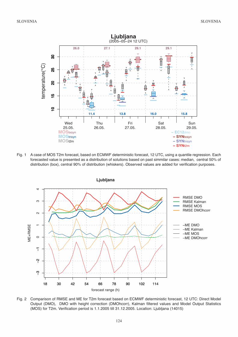
SLOVENIA SLOVENIA
Ljubljana te
mpe
ratu
re(°
C)
(2005−05−24 12 UTC)
Wed Thu Fri Sat Sun25.05. 26.05. 27.05. 28.05. 29.05.
1015
2025
30
MOStxsyn− SYNtxsyn
1015
2025
3026.0
1015
2025
3027.1
1015
2025
3029.1
1015
2025
3029.1
MOStnsyn− SYNtnsyn
1015
2025
30
11.4
1015
2025
30
13.8
1015
2025
30
16.0
1015
2025
30
15.8
MOSt2m− SYNt2m
1015
2025
3010
1520
2530
1015
2025
3010
1520
2530
1015
2025
3010
1520
2530
1015
2025
3010
1520
2530
1015
2025
3010
1520
2530
1015
2025
3010
1520
2530
1015
2025
3010
1520
2530
1015
2025
3010
1520
2530
1015
2025
3010
1520
2530
1015
2025
3010
1520
2530
1015
2025
3010
1520
2530
1015
2025
3010
1520
2530
1015
2025
3010
1520
2530
− EC12dmo
124
Fig. 1 A case of MOS T2m forecast, based on ECMWF deterministic forecast, 12 UTC, using a quantile regression. Eachforecasted value is presented as a distribution of solutions based on past simmilar cases: median, central 50% ofdistribution (box), central 90% of distribution (whiskers). Observed values are added for verification purposes.
Ljubljana
forecast range (h)
ME
+R
MS
E
18 30 42 54 66 78 90 102 114
−3
−2
−1
01
23
4
18 30 42 54 66 78 90 102 114
−3
−2
−1
RMSE DMORMSE KalmanRMSE MOSRMSE DMOhcorr
−ME DMO−ME Kalman−ME MOS−ME DMOhcorr
Fig. 2 Comparison of RMSE and ME for T2m forecast based on ECMWF deterministic forecast, 12 UTC: Direct ModelOutput (DMO), DMO with height correction (DMOhcorr), Kalman filtered values and Model Output Statistics(MOS) for T2m. Verification period is 1.1.2005 till 31.12.2005. Location: Ljubljana (14015)

SLOVENIA SLOVENIA
125
Maribor
forecast range (h)
ME
+R
MS
E
18 30 42 54 66 78 90 102 114
−1
01
23
18 30 42 54 66 78 90 102 114
−1
01
23 RMSE DMO
RMSE KalmanRMSE MOSRMSE DMOhcorr
−ME DMO−ME Kalman−ME MOS−ME DMOhcorr
Fig. 3 Comparison of RMSE and ME for T2m forecast based on ECMWF deterministic forecast, 12 UTC: Direct ModelOutput (DMO), DMO with height correction (DMOhcorr), Kalman filtered values and Model Output Statistics(MOS) for T2m. Verification period is 1.1.2005 till 31.12.2005. Location: Maribor (14026)
Portoroz
forecast range (h)
ME
+R
MS
E
18 30 42 54 66 78 90 102 114
−1
12
3
18 30 42 54 66 78 90 102 114
−1
0
RMSE DMORMSE KalmanRMSE MOSRMSE DMOhcorr
−ME DMO−ME Kalman−ME MOS−ME DMOhcorr
Fig. 4 Comparison of RMSE and ME for T2m forecast based on ECMWF deterministic forecast, 12 UTC: Direct ModelOutput (DMO), DMO with height correction (DMOhcorr), Kalman filtered values and Model Output Statistics(MOS) for T2m. Verification period is 1.1.2005 till 31.12.2005. Location: Portoroz (14105)

SLOVENIA SLOVENIA
126
010
2030
4050
6070
Ljubljana
forecast range (h)
Ski
ll S
core
(R
MS
E)(
%)
18 30 42 54 66 78 90 102 114
010
2030
4050
6070
18 30 42 54 66 78 90 102 114
010
2030
4050
6070
MOS/DMOMOS/DMOhcorrMOS/Kalman
Fig. 5 Skill Score (RMSE - RMSEref)/(RMSEperf-RMSEref)*100%) of MOS T2m forecast in reference to DMO,DMOhcorr and Kalman forecast, based on ECMWF deterministic forecast, 12 UTC. Verification period is1.1.2005 till 31.12.2005. Location: Ljubljana (14015)

SPAIN SPAIN
Verification of ECMWF products in Spain
1. Summary of major highlights of use and verification.
2. Verification of products.
2.1 Objective verification
2.1.1 Direct ECMWF model output (both deterministic and EPS)
2.1.2 ECMWF model output compared to other NWP used by your service.
2.1.3 Post-processed products:
a) Temperature verification
Extensive verification of the objective local deterministic forecasts of daily maximum and minimum temperature up to tendays in advance, obtained by filtering of the 2m-temperature ensemble mean values has continued during 2005. The globalresults of this systematic verification for a set of 50 selected synoptic stations over the Spanish territory are included in amonthly summary report for internal use, in the same way that was produced in previous years. Some of the verification resultsobtained for the period January – December 2005 are depicted in figures 1 to 4.
b) Wind gust estimation and verification
Several methods for wind gust estimation (only the turbulent component) has been tested from the outputs of HIRLAMnumerical model (Vindel et al., 2006). The different methods tested are: ECMWF method (2004), Brasseur (2001), KNMImethod (code from Ben W. Schreur), DWD method and INM rule of thumb. The results indicate no big differences betweenthe different methods compared, being the ECMWF method the one that obtains the best results. Other conclusion is that thedifferent methods tested shouldn’t be used directly to forecast the overcoming of some thresholds because the probabilitiesof detection obtained are poor and the false alarms high. The frequency distributions obtained for every category of forecastwind gust could be an important tool to make probabilistic estimations of wind gusts and to fix maximum thresholds for gustsunder some probability conditions. Some of this verification results are shown in next figures, 5 to 10.
2.2 Subjective verification
Seasonal Forecasts:
ReferencesBrasseur, O., 2001: Development and Application of a Physical approach to Estimating Wind Gusts, Mon. Wea. Rev.,129, 5-25
ECMWF, 2004: IFS Documentation CY28r1. http://www.ecmwf.int/research/ifsdocs/CY28r1/Physics/index.html
Vindel, J.M.; Calvo, J; Del Hoyo, J.; 2006: Evaluación de distintos métodos de predicción de rachas de viento; XXIX JornadasCientíficas de la Asociación Meteorológica Española.
127

SPAIN SPAIN
Fig. 1 Time series of monthly mean values of RMSE for objective maximum temperature forecasts for different predic-tion ranges during 2005. Local forecasts are obtained from the filtering of the 2m-Temp EPS mean. The verifica-tion sample is composed by the forecasts for a set of 50 Spanish synoptic stations.
128
Fig. 2 Time series of percentage of correct maximum temperature forecasts (error less than 2ºC) for different pre-diction ranges. The verification sample is composed by the forecasts made in 2005 for a set of 50 SpanishSYNOP stations.

SPAIN SPAIN
129
Fig. 3 Time series of monthly mean values of RMSE for objective minimum temperature forecasts for different predic-tion ranges during 2005. Local forecasts are obtained from the filtering of the 2m-Temp EPS mean. The verifi-cation sample is composed by the forecasts for a set of 50 Spanish synoptic stations.
Fig. 4 Time series of percentage of correct minimum temperature forecasts (error less than 2ºC) for different predictionranges. The verification sample is composed by the forecasts made in 2005 for a set of 50 Spanish SYNOP stations.

SPAIN SPAIN
Table 1 R2 coefficients, for the different methods compared.
130
HIRLAM 0.16 HIRLAM 0.05
n R2 n R2
BRASSEUR 44524 0.51 39206 0.57
BRAS min. 44524 0.50 39206 0.57
BRAS max. 44524 0.47 39206 0.54
DWD 44524 0.49 39192 0.54
ECMWF 44524 0.54 39206 0.59
INM 44524 0.45 39192 0.51
INM max. 44524 0.36 39192 0.45
KNMI 44524 0.52 39192 0.58
Fig. 5 RMSE and bias function of observed wind gust.

SPAIN SPAIN
131
Fig. 6 RMSE and bias function of forecast length, for observed wind speed > 20 km/h.
Fig. 7 RMSE and bias function of forecast length, for observed wind speed > 40 km/h.

SPAIN SPAIN
132
Fig. 8 Probabilities of detection for the different methods.
Fig. 9 False alarm rates for the different methods.

SPAIN SPAIN
133
Fig. 10 Frequency distributions for the different forecast wind gust categories, using the ECMWF method. Percentiles 5, 25, 50, 75 y 95 are represented.
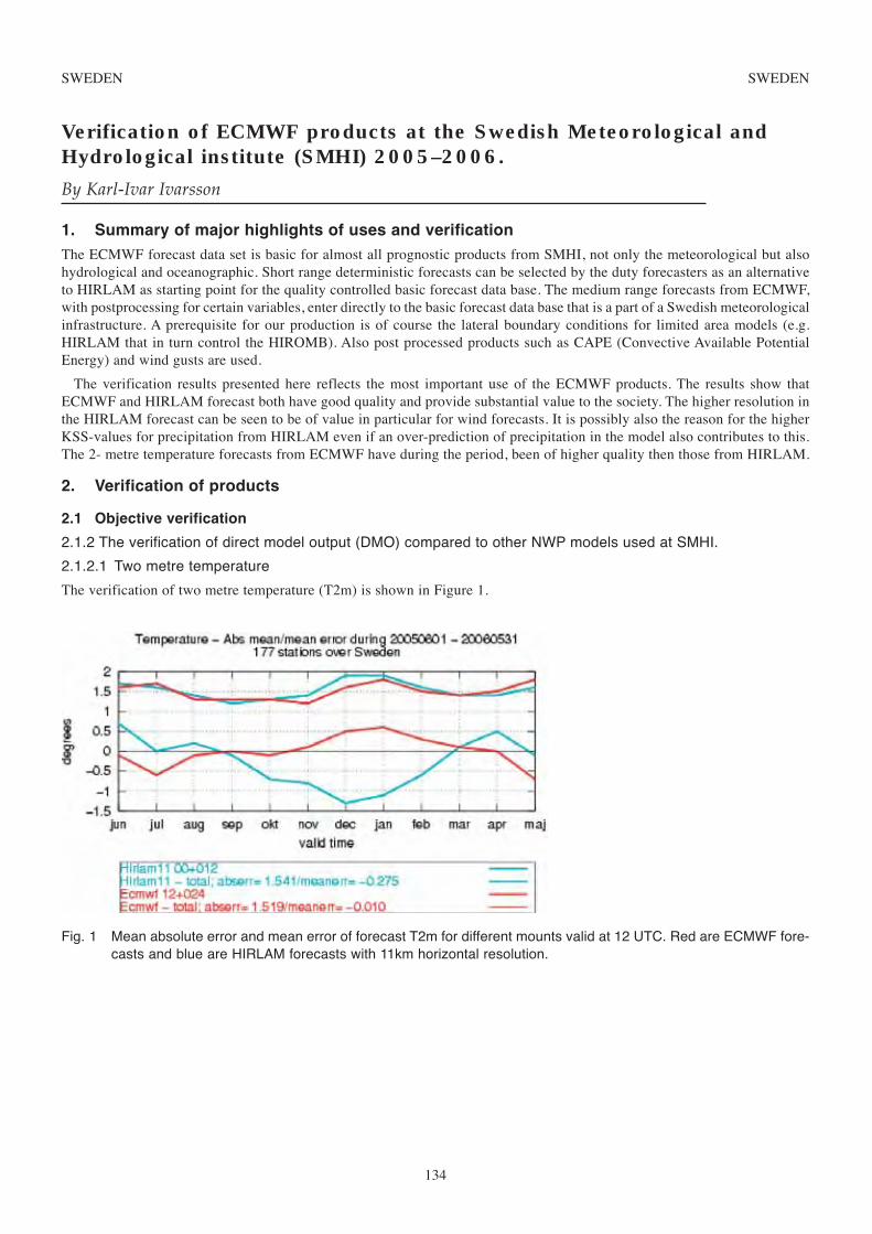
SWEDEN SWEDEN
Verification of ECMWF products at the Swedish Meteorological andHydrological institute (SMHI) 2005–2006.By Karl-Ivar Ivarsson
1. Summary of major highlights of uses and verificationThe ECMWF forecast data set is basic for almost all prognostic products from SMHI, not only the meteorological but alsohydrological and oceanographic. Short range deterministic forecasts can be selected by the duty forecasters as an alternativeto HIRLAM as starting point for the quality controlled basic forecast data base. The medium range forecasts from ECMWF,with postprocessing for certain variables, enter directly to the basic forecast data base that is a part of a Swedish meteorologicalinfrastructure. A prerequisite for our production is of course the lateral boundary conditions for limited area models (e.g.HIRLAM that in turn control the HIROMB). Also post processed products such as CAPE (Convective Available PotentialEnergy) and wind gusts are used.
The verification results presented here reflects the most important use of the ECMWF products. The results show thatECMWF and HIRLAM forecast both have good quality and provide substantial value to the society. The higher resolution inthe HIRLAM forecast can be seen to be of value in particular for wind forecasts. It is possibly also the reason for the higherKSS-values for precipitation from HIRLAM even if an over-prediction of precipitation in the model also contributes to this.The 2- metre temperature forecasts from ECMWF have during the period, been of higher quality then those from HIRLAM.
2. Verification of products
2.1 Objective verification
2.1.2 The verification of direct model output (DMO) compared to other NWP models used at SMHI.
2.1.2.1 Two metre temperature
The verification of two metre temperature (T2m) is shown in Figure 1.
134
Fig. 1 Mean absolute error and mean error of forecast T2m for different mounts valid at 12 UTC. Red are ECMWF fore-casts and blue are HIRLAM forecasts with 11km horizontal resolution.

SWEDEN SWEDEN
During this winter the HIRLAM forecasts have suffered from having a severe negative bias, but after the introduction of anew version of the model in the beginning of Mars, this problem seems to have been solved. ECMWF forecast have been ofa good quality this winter, except for a slightly positive bias. This positive bias is mainly due to errors in forecasts of verylow temperatures. This can be seen in Figure 2.
135
Fig. 2 Frequencies of forecast T2m. Grey observed, red ECMWF and blue HIRLAM.
The frequencies of the T2m forecasts from HIRLAM 11 correspond better to the observed ones than the ECMWF forecastsfor low temperatures (below -15). The same characteristic is seen for high temperatures (above +25). The correspondencewith observed frequencies is mainly good between +5 and -15 for the ECMWF forecasts, and better than HIRLAM nearfreezing point. The reason for the two maxima of the frequencies in Figure 2 is that forecasts valid at 00 UTC and 12 UTCare put together.
2.1.2.2 Ten metre wind speed
The verification of ten metre wind speed (W10m) is seen in Figure 3.
Fig. 3 Mean absolute error and mean error of forecast W10m for different months valid at 12 UTC. Red are ECMWFforecasts and blue are HIRLAM forecasts with 11km horizontal resolution.

SWEDEN SWEDEN
The HIRLAM forecasts are generally somewhat better, if we accept mean absolute error as a measure of forecast quality.This is also seen during the cold season, despite the positive bias of 0.5 to 1m/s of the HIRLAM forecasts. Also the ECMWFforecasts have a positive bias but only about a quarter of a meter per second. The correspondence between the observedfrequencies of wind speed and the ECMWF forecasts is fairly good, which can be seen in Figure 4. But both high and lowwind speeds are of too low frequency. HIRLAM is even worse for low wind speeds but performs fairly well for high ones.The performance of the models by using the Kuipers Skill score (KSS) is seen in Figure 5.
136
Fig. 4 Frequencies of forecast W10m for coastal stations. Grey observed, red ECMWF and blue HIRLAM.
Fig. 5 Forecast value as expressed by KSS for different threshold values. Red ECMWF and blue HIRLAM. The verti-cal bars indicate the uncertainty of the KSS values.
The KSS values of ECMWF and HIRLAM and are mainly the same for low wind speeds, but those from HIRLAM arebetter for high wind speeds.
2.1.2.3 Precipitation
Different amounts of observed and forecast precipitation are compared in Figures 6 and 7.

SWEDEN SWEDEN
Both figures show that there is too much precipitation in the models compared to observations, but the largest difference isseen for HIRLAM during winter. Some of those differences are caused by measurement errors.
The results if KSS is used as the verification score are seen in Figures 8 and 9.
137
Fig. 6 Frequencies of 12 hour precipitation for summer 2005. Red ECMWF, blue HIRLAM and grey observations.
Fig. 7 Frequencies of 12 hour precipitation for winter 2006. Red ECMWF, blue HIRLAM and grey observations.

SWEDEN SWEDEN
There are higher KSS values for the HIRLAM forecasts for the largest amount of precipitation. This is partly due to thehigher forecast frequency of those amounts.
2.1.2.4 Verification of extended HIRLAM forecasts compared to ECMWF.
HIRLAM with 11km resolution currently runs up to 72 hours. Those long forecasts are intended to be used for an evaluationof the quality of lagged EPS with HIRLAM. Here, a brief test of the performance of the longer forecasts is done (Figure 10).
138
Fig. 8 Forecast value as expressed by KSS for different threshold values, summer 2005. Red ECMWF and blueHIRLAM. The vertical bars indicate the uncertainty of the KSS values.
Fig. 9 Forecast value as expressed by KSS for different threshold values, winter 2006. Red ECMWF and blue HIRLAM.The vertical bars indicate the uncertainty of the KSS values.
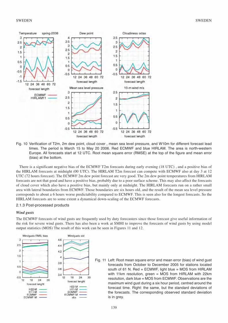
SWEDEN SWEDEN
There is a significant negative bias of the ECMWF T2m forecasts during early evening (18 UTC) , and a positive bias ofthe HIRLAM forecasts at midnight (00 UTC). The HIRLAM T2m forecast can compete with ECMWF also at day 3 at 12UTC (72 hours forecast). The ECMWF 2m dew point forecast are very good. The 2m dew point temperatures from HIRLAMforecasts are not that good and have a positive bias, probably due to a poor surface scheme. This may also affect the forecastsof cloud cover which also have a positive bias, but mainly only at midnight. The HIRLAM forecasts run on a rather smallarea with lateral boundaries from ECMWF. Those boundaries are six hours old, and the result of the mean sea level pressurecorresponds to about a 6 hours worse predictability compared to ECMWF. This is seen also for the longest forecasts. So theHIRLAM forecasts are to some extent a dynamical down-scaling of the ECMWF forecasts.
2.1.3 Post-processed products
Wind gusts
The ECMWF forecasts of wind gusts are frequently used by duty forecasters since those forecast give useful information ofthe risk for severe wind gusts. There has also been a work at SMHI to improve the forecasts of wind gusts by using modeloutput statistics (MOS) The result of this work can be seen in Figures 11 and 12.
139
Fig. 10 Verification of T2m, 2m dew point, cloud cover , mean sea level pressure, and W10m for different forecast leadtimes. The period is March 15 to May 20 2006. Red ECMWF and blue HIRLAM. The area is north-westernEurope. All forecasts start at 12 UTC. Root mean square error (RMSE) at the top of the figure and mean error(bias) at the bottom.
Fig. 11 Left: Root mean square error and mean error (bias) of wind gustforecasts from October to December 2005 for stations locatedsouth of 61 N. Red = ECMWF, light blue = MOS from HIRLAMwith 11km resolution, green = MOS from HIRLAM with 22kmresolution, dark blue = MOS from ECMWF. Observations are themaximum wind gust during a six hour period, centred around theforecast time. Right: the same, but the standard deviations ofthe forecasts. The corresponding observed standard deviationis in grey.

SWEDEN SWEDEN
The MOS does a good job for all models, and seems to be somewhat better than ECMWF post-processed wind gusts. Thehigh KSS values for the HIRLAM 11 MOS forecasts are partly due to be more realistic statistical distribution of the forecasts,which can be seen both in Figure 11 to right where the standard deviations are plotted for the different forecasts and in Figure12, where the different frequencies are plotted.
2.2 Subjective verification
2.2.2 Evaluation of the behaviour of the model
The duty forecasters are to mostly very happy with the forecasts. There are some less good characteristic however, that maybe worth noticing.
• Too small amount of cloudiness in case of convection, especially convective precipitation in the summertime
• Too large amount of low clouds in case of very cold weather in winter ( below -20 degrees Celsius)
• Too much fog over cold sea, especially in spring. There is also often too low T2m in the areas of such fog.
140
Fig. 12 KSS values for different thresholds for wind gust forecasts, The verification period is October to December 2005,for stations located south of 61 N. Red = ECMWF, light blue = MOS from HIRLAM with 11km resolution, green =MOS from HIRLAM with 22km resolution, dark blue = MOS from ECMWF. Observations are the maximum windgust during a six hour period, centred around the forecast time. The observed relative frequencies in grey.

SWITZERLAND SWITZERLAND
Verification of ECMWF products at MeteoSwissAuthors: Mark Liniger
1. Summary of major highlightsMeteoSwiss has continued to use seasonal forecasts of System 2 and to evaluate the potential seasonal predictability. Seasonalforecast skill and the potential predictability have been evaluated on a grid-point scale and over Switzerland. A revised skillscore was developed which eliminates the negative bias of the ranked probability skill score for ensembles of finite size.
2. Verification products
2.1 Objective Verification
2.1.1
2.1.2
2.1.3
2.1.4
2.1.5 Seasonal forecasts (Mark Liniger)
Here, the forecast skill (RPSSd, Müller, 2004; Müller et al., 2005b; Weigel et al., 2006) of the 2m mean temperature is examinedfrom a grid-point perspective. Figure 1 shows an example of the potential seasonal predictability of the operational ECMWFseasonal forecast system 2 for the period 1987-2002 (Schwierz et al., 2006). For the verification ERA-40 reanalysis data areused (Fig. 1a). High skill scores are found over the oceans, in particular over the tropics. Highest values are located in the ElNino region in the eastern tropical Pacific, whereas the western Pacific, the Indian Ocean and the tropical Atlantic showsomewhat lower, but mostly significant positive skill. The heterogeneous patterns in the region of Indonesia are mostly dueto the differences between the land-sea masks of the forecast model and the verification data set (ERA40). In the extratropics,the Pacific basin exhibits wide regions of significant skill. For the Atlantic basin, the values are closer to zero. Relevant forEurope, there is a bandlike structure of a weak positive signal across the northern Atlantic reaching from Newfoundland tothe Bay of Biscay. Over land, the skills are lower throughout. Highest values are found over Northern America, and along thePacific coast of Asia. Most other continents, in particular Europe, are associated with negative or non-significant values.
The estimated potential predictability (PMA) supports these findings (Fig. 1b, Schwierz et al., 2006). The tropical oceansfeature high potential predictability. In the extratropics, the oceans show reduced but still significant positive values. Overland, the PMA implies a higher predictability in the tropics than extratropics (e.g. over Africa and Southern America). Acomparison to the verification against ERA40 shows, that this potential is not “realized” in the actual forecast skill. A betteragreement between the potential predictability and the actual skill is found in the extratropics with very limited, but significant,skill values. In particular over the European region the skill scores are in the order of less then 10%, both for PMA and theactual skill.
Further, the skill of the ECMWF System has been analysed over Switzerland in more detail. The RPSSd for the 3-monthlyaverage is shown for the period 1987 - 2004 for 2m temperature. The skill of the System 2 strongly varies over the seasons.Highest skill scores are achieved for the forecasts started in late spring and early summer, covering the summer months. Lowestskill can be found for autumn and winter.
141
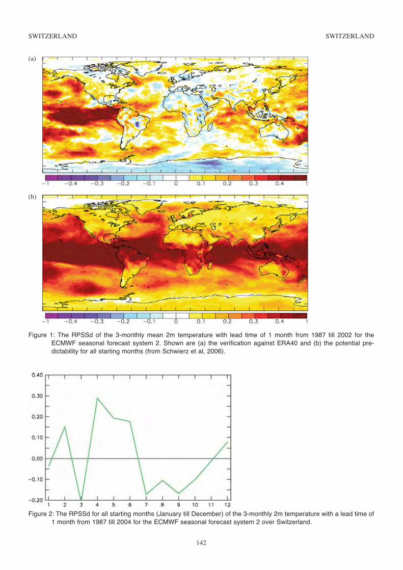
Figure 2: The RPSSd for all starting months (January till December) of the 3-monthly 2m temperature with a lead time of1 month from 1987 till 2004 for the ECMWF seasonal forecast system 2 over Switzerland.
SWITZERLAND SWITZERLAND
142
(a)
(b)
Figure 1: The RPSSd of the 3-monthly mean 2m temperature with lead time of 1 month from 1987 till 2002 for theECMWF seasonal forecast system 2. Shown are (a) the verification against ERA40 and (b) the potential pre-dictability for all starting months (from Schwierz et al, 2006).

SWITZERLAND SWITZERLAND
143
2.2 Subjective Verification
3. ReferencesLiniger, Mark A., 2003: Wetter- und Klimastuerme. GAIA 12 (2003) no.4, 260-265.
Liniger M. A., C. Appenzeller, 2006: Switzerland Long Range Forecasting Progress Report of MeteoSwiss for 2004. WMO
Müller, W., 2004: Analysis and Prediction of the European Winter Climate, Dissertation, ETH Zürich Nr. 15540, inVeröffentlichung der MeteoSchweiz, Nr. 69, pp101.
Müller, W. A., M. A. Liniger, M. A., C. Appenzeller, 2004: Switzerland Long Range Forecasting Progress Report ofMeteoSwiss for 2003.
Mueller, W., C. Appenzeller and C. Schaer, 2005a: Probabilistic seasonal prediction of the winter North Atlantic Oscillationand its impact on near surface temperature, Climate Dynamics, DOI: 10.1007/s00382-004-0492-z 02.2005.
Mueller W. A., C. Appenzeller, F. J. Doblas-Reyes, M. A. Liniger, 2005b: A debiased ranked probability skill score to evaluateprobabilistic ensemble forecasts with small ensemble sizes, Journal of Climate, 18 (10), 1513-1523.
Schwierz, C., C. Appenzeller, H. C. Davies, M. A. Liniger, W. Müller, T. F. Stocker and M. Yoshimori, 2006: Multi-decadalClimate Projections to Seasonal and Sub-seasonal Predictions: An Overview of the Challenges. Clim. Change, in press.
Weigel A.P., M. A. Liniger, C. Appenzeller, 2006: The discrete Brier and ranked probability skill scores. Mon. Wea. Rev.(accepted)

TURKEY TURKEY
Application and Verification of ECMWF products in Turkey 2005Turkish State Meteorological Service - Ankara / Turkey
1. Summary of major highlights
2. Verification of Products
2.1 Objective Verification
2.1.1 Direct ECMWF Model Outputs
24 hourly forecasts between T+00 and T+144 of 12 UTC and 00 UTC deterministic model are operationally verified by usingstandard statistical scores (mean error, root mean square error and mean absolute error). For the verification of all parameters,60 Turkish synoptic stations were used, covering the period from January to December 2005.
(i) In the free atmosphere
In order to verify upper level parameters, verification are performed against to observations at 7 radio-sonde stations. ECMWFanalysis at pressure levels were used for other stations.
(ii) Local weather parameters
Local weather parameters used in report are daily maximum and minimum, 2 meter temperature values observed at 12 UTC,mean sea level pressure, and total precipitation. The model outputs interpolated to the station points are verified againstcorresponding observations. For this process, suitable time steps of model outputs were used. Verified parameters and its periodsfor the year 2005 are given in below:
• Daily Maximum and Minimum Temperature; D+1, D+2, ..., D+7;Scores: ME, RMSE, MAE.
• Mean Sea Level Pressure and 2 m Temperature: D+1, D+2, ..., D+7;Scores: ME, RMSE, MAE.
• Total Precipitation existence and contingency tables with 6 categories (0, 0.1-1, 1-5, 5-10,10-20, 20<mm): D+1, D+2, D+3;Scores: BIAS, HIT, FAR, TS, POD.
• 1000, 850, 700, 500 and 300 hPa Height and Temperature: D+1, D+2, ..., D+7;Scores: ME, RMSE, MAE.
144
Fig. 2.1.1.1 Turkish synoptic and radio-sonde stations used in this study

TURKEY TURKEY
145
Fig. 2.1.1.2 12 UTC RMSE Values of Minimum Temperature D+1
Fig. 2.1.1.3 12 UTC RMSE Values of Minimum temperature for D+6
Fig. 2.1.1.4 00 UTC RMSE Values of 2M Temperature for D+2

TURKEY TURKEY
146
Fig. 2.1.1.5 00 UTC RMSE Values of 2M Temperature for D+4
Fig. 2.1.1.6 12 UTC RMSE Values of Mean Sea Level Pressure for D+1
Fig. 2.1.1.7 12 UTC RMSE Values of Mean Sea Level Pressure for D+4

TURKEY TURKEY
147
Fig. 2.1.1.8 00 UTC RMSE Values of Maximum Temperature for D+5
Fig. 2.1.1.9 Root Mean Square Errors of 00 and 12 UTC 2m Temperature forecasts as a function of forecast range for7 Turkish radio-sonde stations
Fig. 2.1.1.10 Root Mean Square Errors of 00.00 and 12.00 UTC MSL Pressure forecasts as a function of forecast rangefor 7 Turkish radio-sonde stations

Ankara (D+3)
93 81 far=0.47 bias=1.66
12 142 hit=0.72 ts=0.50
pod=0.89
Ankara (D+2)
94 68 far=0.42 bias=1.54
11 155 hit=0.76 ts=0.54
pod=0.90
Adana (D+3)
49 118 far=0.71 bias=3.27
2 149 hit=0.62 ts=0.29
pod=0.96
TURKEY TURKEY
148
Fig. 2.1.1.11 Root Mean Square Errors of 00.00 and 12.00 UTC 850 hPa Height forecasts as a function of forecastrange for 7 Turkish radio-sonde stations
Verification of Precipitation
Precipitation forecasts of the ECMWF are interpolated to the station points. Interpolated model outputs and correspondingobservations are compared. 24 hourly total precipitation values are classified as follows;
Adana (D+1)
48 106 far=0.69 bias=3.02
3 161 hit=0.66 ts=0.31
pod=0.94
Observation
Yes No
Forecast Yes a b
No c d
FAR = b/(a+b)Hit Rate = (a+d)/(a+b+c+d)BIAS = (a+b)/(a+c)POD = a/(a+c)TS = a/(a+b+c)

TURKEY TURKEY
149
2.1.2 ECMWF model output compared to other NWP models
MM5 model is running four times in a day for various mesh-size, domains and ranges. The boundary conditions are receivedthrough ECMWF BC project. Verification of MM5 outputs such as MSL pressure, 2m temperature, 10 meter u-v windcomponents and total precipitation parameters for 12 UTC run are performed against observations. However, objectivecomparison has not been performed between ECMWF and MM5 so far. According to subjective comparison, 2metertemperature values of ECMWF produce more accurate scores than those of MM5. Whereas, MM5 model forecasts for thetotal precipitation are generally better than ECMWF.
2.1.3 Post-processed products
Kalman Filtering
Kalman Filtering is applied to 101 stations including 31 foreign stations from D+1 to D+4 for 2-meter maximum and minimumtemperatures. Kalman Filtering scores of some stations are given in below:
Fig. 2.1.1.12 HIT Rates of Total Precipitation (00 UTC Run) for D+1
Fig. 2.1.1.13 HIT Rates of Total Precipitation (00 UTC Run) for D+3

TURKEY TURKEY
150
Fig. 2.1.3.1 Comparison of the 2 meter Maximum Temperature (12 UTC run) values of Kalman Filtering to DMO ofIstanbul for D+2
Fig. 2.1.3.2 Comparison of the 2m Minimum Temperature (12 UTC run) values of Kalman Filtering to DMO of Ankarafor D+1

TURKEY TURKEY
151
Fig. 2.1.3.3 Comparison of the 2m Minimum Temperature (12 UTC run) values of Kalman Filtering to DMO of Izmirfor D+3
Fig. 2.1.3.4 Filtered RMSE Values of Minimum Temperature for D+1

TURKEY TURKEY
152
Fig. 2.1.3.5 Filtered RMSE Values of Maximum Temperature for D+2
2.1.4 End Products delivered to users
None.
2.1.5 Seasonal forecasts
None.
2.2 Subjective verification
2.2.1 Subjective scores
Our Weather Analysis and Forecasting Division (WAFD) uses ECMWF outputs for wide range of purposes from short-rangeforecasts to the special reports. We compared ECMWF forecasts and those of WAFD forecasts (based on bench forecasters’experience) with observed values. The verification results were based on the observed values received from 41 stationsthroughout Turkey and ECMWF’s D+1, D+2, D+3 and D+4 corresponding forecasts. When “yes-no” type of verificationapplied for ECMWF precipitation forecasts, little improvements were noted. Most of the figures show a continuing upwardtrend over the past few years. Based on ECMWF’s upward trend, with combining their experiences and ECMWF model outputs,WAFD has issued better precipitation forecasts than previous years.
2.2.2 Synoptic Studies, evaluation of the behavior of the model
None
2.2.3 Seasonal Forecasts
None
2.2.4 Monthly Forecasts
None
3. ReferencesECMWF, (2005): Verification of ECMWF products in Member States and Co-operating States, Report 2004.
Güser, A. (2004): (in Turkish) “Kalman Filtresi ve Türkiye Üzerine Uygulamaları”, Turkish State Meteorological Service,Ankara, p17-40.
Güser, A. (2002): (in Turkish) “Verifikasyon ve Türkiye Üzerine Uygulamaları”, Turkish State Meteorological Service,Ankara, p13-23.
Kocaman, F. (2002): (in Turkish) “Kalman Filter ve Türkiye Üzerine Uygulamaları”, Turkish State Meteorological Service,Ankara, p9-12.

UNITED KINGDOM UNITED KINGDOM
Verification of ECMWF Products at the Met Office, Exeter, UK
1. Summary of major highlights
2. Verification of products
2.1 Objective verification
2.1.1 Direct ECMWF model output
2.1.1 (i) in the free atmosphere
ECMWF and Met Office forecast fields of PMSL, 500 hPa height and 250 hPa wind have been verified against observations.Monthly mean RMS errors for an area covering Western Europe, the North Atlantic and North America are plotted in ANNEXA, Figures 2.1.1(i)a,b,c.
Latest resultsPMSL and 500hPa height; During 2005 and 2006 ECMWF remains ahead of the Met Office at T+72 and 120. However, atT+24 the Met Office improves relatively and almost catches up by March 2006.
250 hPa wind; ECMWF remains ahead at all forecast ranges but with the Met Office catching up slowly with time.
2.1.1 (ii) of local weather parameters verified for locations which are of interest to your service
Nothing to report.
2.1.1 (iii) of oceanic waves
The Met Office continues to contribute to the monthly verification exchange of global wave models.
2.1.2 ECMWF model output compared to other NWP models used by the Met Office
Verification and Intercomparison of ECMWF Tropical Cyclone Forecasts
The Met Office has been carrying out verification of its own tropical cyclone (TC) forecast track errors since 1988 and ofthose from ECMWF since 1994. In addition, verification of the intensity tendency of TC forecasts has been carried out since2001. The latter is done by a simple method which determines whether the model is forecasting weakening or strengtheningover each 24 hour period based on model values of 850hPa relative vorticity at the TC centre. A skill score is produced toindicate whether the model is better than chance.
Results of an intercomparison between Met Office and ECMWF TC forecasts were presented in this report two years agofor the period May 2003 to April 2004. These included track forecast errors, weakening, strengthening and intensity tendencyskill scores. An update is included in this report to cover the full period from 1994 to 2005 for TC track errors and 2001 to2005 for intensity tendency errors. All comparisons are for homogeneous datasets.
Globally averaged track forecast errors for the Met Office global and ECMWF models can be seen in Figure 1 (T+24, 48and 72) and Figure 2 (T+96 and 120). These firstly indicate a downward trend in track forecast errors for both the Met Officeand ECMWF models. 72-hour forecast errors in 2005 were near to the 36-hour forecast errors in 1994. The Met Office hasmaintained its advantage over ECMWF in track prediction at T+24 and T+48, although the gap has narrowed in recent years.At T+72 Met Office and ECMWF errors have each been the lowest in six of the 12 years. However, ECMWF has been lowerthan the Met Office in three of the last four years. Relative performance has always been mixed at the longer lead times ofT+96 and T+120. However, the gap between ECMWF and the Met Office has widened in favour of ECMWF in the last coupleof years.
Globally and lead-time averaged intensity skill scores for the Met Office and ECMWF models can be seen in Figure 3. Interms of overall intensity tendency there is very little difference between the Met Office and ECMWF. Both show a positiveintensity tendency rising from between 10 and 20% to between 20 and 30% during the five year period. However, when thisintensity tendency is broken down into strengthening and weakening skill, large differences between the two models appear.ECMWF show a much greater level of skill in predicting strengthening, which has risen about 20% during the five year period.The Met Office strengthening skill started from a base point almost 80% below ECMWF. However, the tendency to weakenTCs too quickly was partially addressed by the 2002 ‘New Dynamics’ model upgrade (Heming and Greed, 2002). Since thenthe strengthening skill has risen consistently and at about twice the rate of ECMWF. Met Office weakening skill wasapproximately 40% higher than ECMWF during the five year period. There was only a slight change in relative performanceduring the period with the difference between the two skill scores narrowing slightly.
In summary, Met Office short period track forecast errors are lower than ECMWF, although the gap is narrowing. At longerlead times ECMWF track forecast errors are generally lower. Both models show similar intensity tendency skill scores, butECMWF is better at predicting strengthening, whilst the Met Office is better at predicting weakening.
153

Fig. 3
UNITED KINGDOM UNITED KINGDOM
154
Fig. 1
Met Office v. ECMWF GlobalTropical Cyclone Track Forecast Errors
0
100
200
300
400
500
600
1994 1995 1996 1997 1998 1999 2000 2001 2002 2003 2004 2005
Mea
n E
rror
(km
)
Met Office T+24
ECMWF T+24
Met Office T+48
ECMWF T+48
Met Office T+72
ECMWF T+72
Fig. 2
Met Office v. ECMWF Global
Tropical Cyclone Track Forecast Errors900
800
700
600
500
400
300
1994 1995 1996 1997 1998 1999 2000 2001 2002 2003 2004 2005
Mea
n E
rror
(km
)
Met Office T+96
ECMWF T+96
Met Office T+120
ECMWF T+120
Met Office v. ECMWF Global
Tropical Cyclone Intensity Skill Scores
0
80
60
40
20
-20
-40
-602001 2003 2004 20052002
Ski
ll S
core
(%
)
Met Officetendency
ECMWFtendency
Met Officeweakening
ECMWFstrengthening
Met Officestrengthening
ECMWFweakening

UNITED KINGDOM UNITED KINGDOM
155
2.1.3 Post-processed products
2.1.4 End products delivered to users
2.1.5 Seasonal forecasts
2.1.6 Monthly forecasts
2.2 Subjective verification
2.2.1 Subjective scores
Medium-range verification - 2005 results
Introduction
Subjective verification of numerical output from the UKMO Global Model (GM), both raw and modified output, and ECMWF(EC) has continued to be carried out daily in the Operations Centre. This report presents the results for 2005, comparing andhighlighting performances of the models.
Summary
Days 2 to 4, a marked improvement for all models compared to 2004, most notably for Raw GM on Day 2 and for ModifiedGM on Days 3 and 4. For Day 5, continued improvement for EC but slightly worse for Raw and Modified GM.
Results – Days 2-5 EC vs GM (and Modified GM)
“GOOD” forecasts (“GOOD” and “USEFUL” forecasts – scores of 8 and 6)
Day 2 All models showed an improvement over 2004 with scores equalling or bettering any since this series began.Most notable, however, was the improvement in Raw GM which, for the first time since 1999, scored higherthan the Modified GM. EC remained a close third.
Day 3 After a relatively poor 2004, 2005 showed a marked improvement for all models. Both Raw and ModifiedGM achieved above 95%, the latter just beating the former, while the EC is only marginally behind with justover 94%.
Day 4 2005 saw improvement for all models, most marked for the Modified GM, with 81.5%, and the EC with 80.6%.However, the Raw GM, although much improved, with 78.5%, was lagging behind its high of 79.5% of 2003.
Day 5 Both Raw and Modified GM, 2005 saw a slight decrease compared to 2004, although the latter was better thanthe former. EC, however, showed a continuing improvement with 58.2%, its best mark since the 59.1% of 2000.
“BAD” forecasts (‘POOR’ and ‘MISLEADING’ forecasts - scores of 2 and 0)
Day 2 As in 2004, no ‘Poor’ and ‘misleading’ forecasts were marked during 2005.
Day 3 A marked improvement for all models compared to 2004, all models with less than 1%. GM was slightly theworst with 0.57%, whilst Modified GM and EC both had 0.27%.
Day 4 A slight improvement compared to 2004 for Modified GM but Raw GM and EC were slightly worse.
Day 5 All models showed a decrease compared to 2004.
Days 6 – 7 ECOperational:-A marked increase in the percentage of ‘GOOD’ forecasts, reaching 25%, the highest since 1995when a score of 32% was recorded. However, the percentage of ‘POOR’ or MISLEADING’ forecasts also roseslightly, whilst ‘INDETERMINATE’ forecasts decreased slightly.
Ensembles:-A slight increase in Good but matched by a more marked increase in ‘INDETERMINATE’ and poorand misleading compared to 2004.
Days 8 – 10 ECOperational:-There was a continued alight increase in the percentage of ‘GOOD’/’USEFUL’ forecasts. Thepercentage of ‘INDETERMINATE’ forecasts remained the same as 2004 whilst there was an increase in‘POOR’ or MISLEADING’
Ensembles:-A slight increase in Good but matched by a more marked increase in ‘INDETERMINATE’ and poorand misleading compared to 2004.

UNITED KINGDOM UNITED KINGDOM
EC vs ENSEMBLES
Days 6 & 7Compared to Ensemble, Operational slightly more ‘GOOD’ forecasts, fewer ‘INDETERMINATE’ but alsomore ‘POOR’ or ‘MISLEADING’.
Days 8 – 10Compared to Ensemble, Operational slightly more ‘GOOD’ forecasts, fewer ‘INDETERMINATE’ but muchhigher percentage of ‘POOR’ or ‘MISLEADING’.
156
Figure 2.2.1a
2.2.2 Synoptic studies, evaluation of the behaviour of the model
2.2.3 Seasonal forecasts
2.2.4 Monthly forecasts
3. ReferencesHeming, J.T. and Greed, G. (2002). The Met Office 2002 model upgrade and expected impact on tropical cyclone forecasts.American Meteorological Society 25th Conference on hurricanes and tropical meteorology (San Diego, USA). pp.180-1.
MEDIUM RANGE SUBJECTIVE VERIFICATION 2005100
90
80
70
60
50
40
30
20
10
0Day 2 (T+48) Day 3 (T+72) Day 4 (T+96) Day 5 (T+120)
GM (Good) ModGM (Good) ECMWF (Good) GM (Poor) ModGM (Poor) ECMWF (Poor)

UNITED KINGDOM UNITED KINGDOM
Fig. 2.1.1 (i)c: RMS vector wind errors at 250hPa, verified against observations over W.Europe, N.Atlantic, N.America:Jan 1999 - Mar 2005, Met Office (dashed line) and ECMWF (solid line).
Fig. 2.1.1(i)b: RMS errors of 500hPa height, verified against observations over W.Europe, N.Atlantic, N.America:Jan 1999 - Mar 2005, Met Office (dashed line) and ECMWF (solid line).
Fig. 2.1.1(i)a: RMS errors of PMSL, verified against observations over W.Europe, N.Atlantic, N.America:Jan 1999 - Mar 2005, Met Office (dashed line) and ECMWF (solid line).
157
ANNEX A
0
1
2
3
4
5
6
7
8
9
Jan-
00
Apr
-00
Jul-0
0
Oct
-00
Jan-
01
Apr
-01
Jul-0
1
Oct
-01
Jan-
02
Apr
-02
Jul-0
2
Oct
-02
Jan-
03
Apr
-03
Jul-0
3
Oct
-03
Jan-
04
Apr
-04
Jul-0
4
Oct
-04
Jan-
05
Apr
-05
Jul-0
5
Oct
-05
Jan-
06
Err
or (
hPa)
UK T+24
UK T+72
UK T+120
EC T+24
EC T+72
EC T+120
0
1
2
3
4
5
6
7
8
9
10
UK T+24
UK T+72
UK T+120
EC T+24
EC T+72
EC T+120
Jan-
00
Apr
-00
Jul-0
0
Oct
-00
Jan-
01
Apr
-01
Jul-0
1
Oct
-01
Jan-
02
Apr
-02
Jul-0
2
Oct
-02
Jan-
03
Apr
-03
Jul-0
3
Oct
-03
Jan-
04
Apr
-04
Jul-0
4
Oct
-04
Jan-
05
Apr
-05
Jul-0
5
Oct
-05
Jan-
06
Err
or (
dam
)
5
10
15
20
25
30
35
40
45
Err
or (
knot
s)
UK T+24
UK T+72
UK T+120
EC T+24
EC T+72
EC T+120
Jan-
00
Apr
-00
Jul-0
0
Oct
-00
Jan-
01
Apr
-01
Jul-0
1
Oct
-01
Jan-
02
Apr
-02
Jul-0
2
Oct
-02
Jan-
03
Apr
-03
Jul-0
3
Oct
-03
Jan-
04
Apr
-04
Jul-0
4
Oct
-04
Jan-
05
Apr
-05
Jul-0
5
Oct
-05
Jan-
06

UNITED KINGDOM UNITED KINGDOM
158


