39
Application Layer Multicast
| Date post: | 30-Dec-2015 |
| Category: |
Documents |
| Upload: | tate-holcomb |
| View: | 55 times |
| Download: | 1 times |

Application Layer Multicast
2
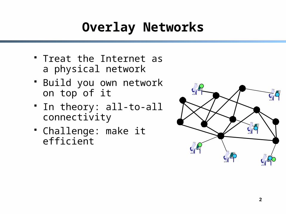
Overlay Networks
Treat the Internet as a physical network
Build you own network on top of it
In theory: all-to-all connectivity
Challenge: make it efficient
3
Example: IP Multicast
Multicast is an efficient delivery mechanism for Group-Communication applications.
IP Multicast - Relay on network layer to replicate and deliver data
packets to receivers.
Problems with IP Multicast- Scales poorly with number of groups
- Supporting higher level functionality is difficult
- Deployment is difficult and slow
4
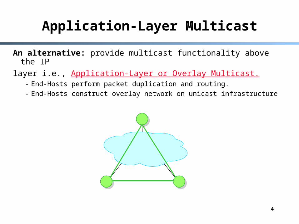
Application-Layer Multicast
An alternative: provide multicast functionality above the IP
layer i.e., Application-Layer or Overlay Multicast.- End-Hosts perform packet duplication and routing.
- End-Hosts construct overlay network on unicast infrastructure
5
Efficiency of Multicast Trees
Challenge: construct efficient overlay trees Application centric performance metrics: delay, throughput Todays focus: delay optimized multicast trees
Naive Solution, Shortest Path Tree (SPT) Does not limit node load Creates bottlenecks (BW and CPU limits)
6
Efficiency of Multicast Trees (cont.)
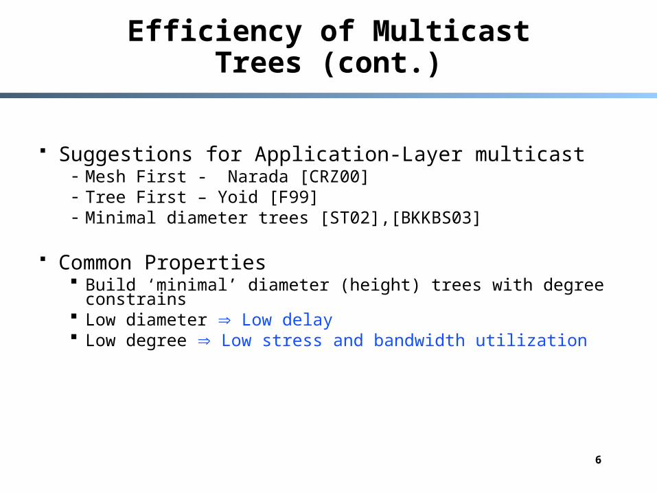
Suggestions for Application-Layer multicast- Mesh First - Narada [CRZ00]- Tree First – Yoid [F99]- Minimal diameter trees [ST02],[BKKBS03]
Common Properties Build ‘minimal’ diameter (height) trees with degree constrains Low diameter Low delay Low degree Low stress and bandwidth utilization

7
Efficiency of Multicast Trees (cont.)
Disadvantages:- Arbitrary selection of degrees
• Requires trial and error- Ignores serialized message distribution
• Scalability problem (known problem [CRZ00])
H3
H1
H2
R1
R2
Low-speed Link
High-speed Links
H3
H1
H2
H3
H1
H2
Non-Optimal Tree Optimal Tree
8
Todays Talk
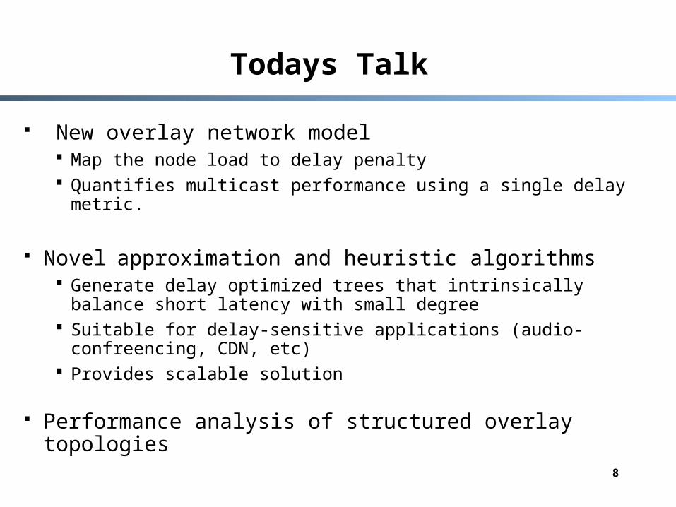
New overlay network model Map the node load to delay penalty Quantifies multicast performance using a single delay metric.
Novel approximation and heuristic algorithms Generate delay optimized trees that intrinsically balance short
latency with small degree Suitable for delay-sensitive applications (audio-confreencing, CDN,
etc) Provides scalable solution
Performance analysis of structured overlay topologies
9
The Overlay Network Model
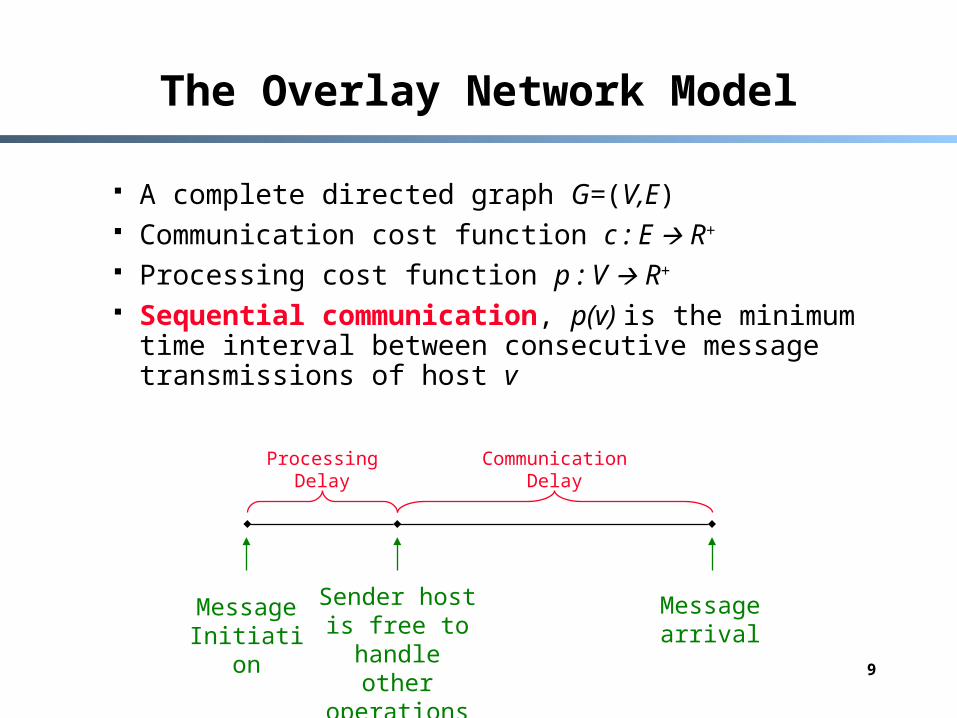
A complete directed graph G=(V,E) Communication cost function c : E R+
Processing cost function p : V R+
Sequential communication, p(v) is the minimum time interval between consecutive message transmissions of host v
Processing Delay
Communication Delay
Message Initiation
Sender host is free to handle
other operations
Message arrival

10
The Minimal Delay Multicast (MDM)Problem
Given a directed complete graph G=(V,E); a multicast group M V; a source host sM; a processing cost p(v), vV; and a communication cost c(e), eE;
Find a scheme that minimizes the delay required to disseminate a message from s to all the other hosts in M. Only the hosts in M are allowed to participate in the distribution
We assume that M≡V Group size n = |V|
11
The Ordered Tree Solution
S
V1 V2
V4 V6V5V3
1
1
12
2
3 3 4 4
3 3
7 8 9 11
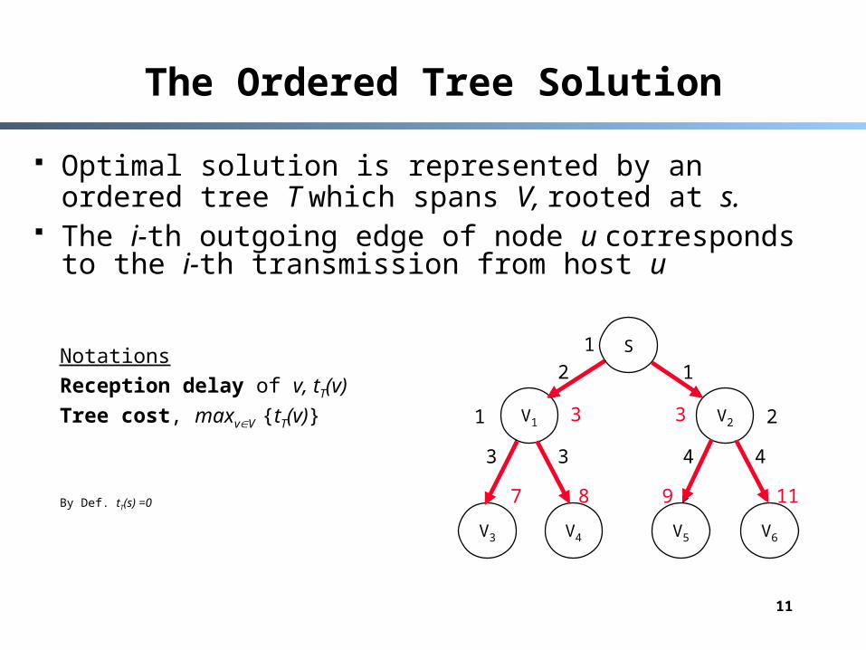
Optimal solution is represented by an ordered tree T which spans V, rooted at s.
The i-th outgoing edge of node u corresponds to the i-th transmission from host u
Notations
Reception delay of v, tT(v)
Tree cost, maxvV {tT(v)}
By Def. tT(s) =0
12
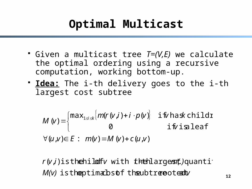
Optimal Multicast
Given a multicast tree T=(V,E) we calculate the optimal ordering using a recursive computation, working bottom-up.
Idea: The i-th delivery goes to the i-th largest cost subtree
vM(v)
m(.)ivivr
vucvMvmEvu
v
kvvpiivrmvM ki
at rooted subtree theofcost optimal theis
quantity largest th - with the of child theis ),(
),()()(:),(
leaf a is if0
children has if)(),((max)( 1
13
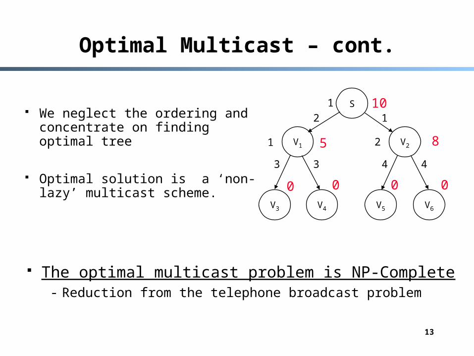
Optimal Multicast – cont.
We neglect the ordering and concentrate on finding optimal tree
Optimal solution is a ‘non-lazy’ multicast scheme.
S
V1 V2
V4 V6V5V3
1
1
12
2
3 3 4 4
5 8
0 0 0 0
10
The optimal multicast problem is NP-Complete- Reduction from the telephone broadcast problem
14
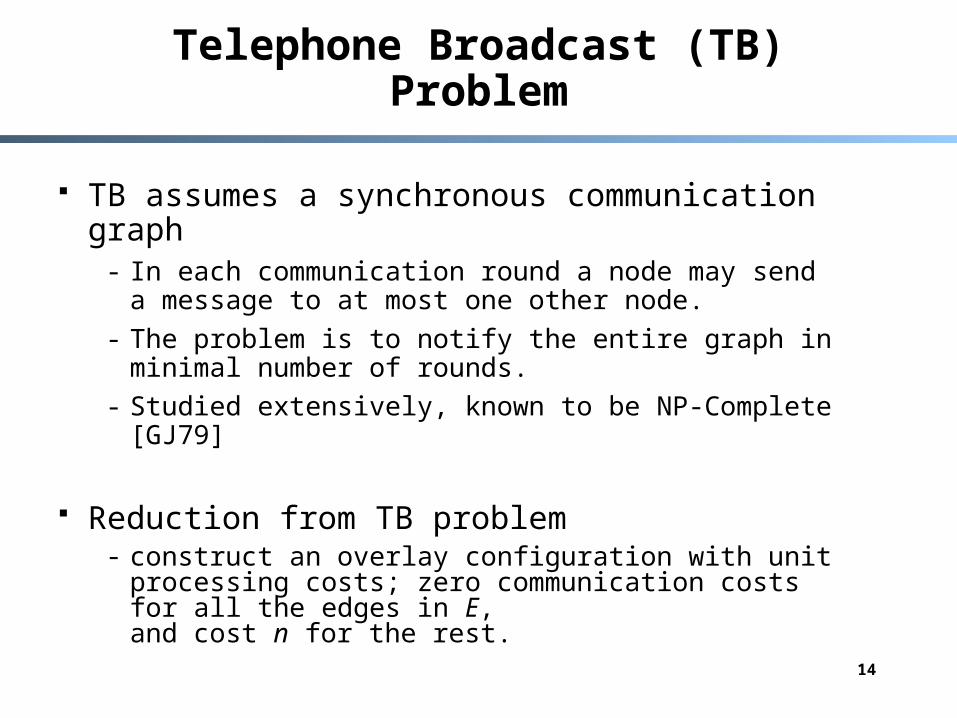
Telephone Broadcast (TB) Problem
TB assumes a synchronous communication graph- In each communication round a node may send a message
to at most one other node.
- The problem is to notify the entire graph in minimal number of rounds.
- Studied extensively, known to be NP-Complete [GJ79]
Reduction from TB problem- construct an overlay configuration with unit processing
costs; zero communication costs for all the edges in E, and cost n for the rest.
15
Computation Models
Homogenous models- Active Networks [RS01]
• Multicasting algorithm for line topologies
The heterogeneous postal model [BGNSS01]- Assumes undirected and complete graph G=(V,E)
- Communication latency function λ
- Switching (sending) time function s
16
Postal Approximation
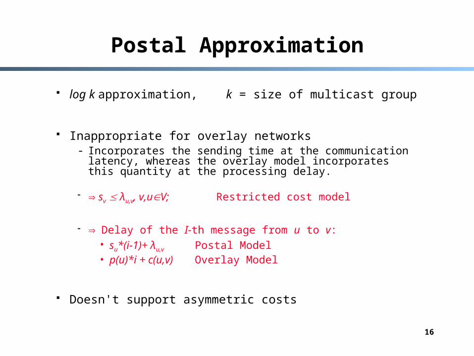
log k approximation, k = size of multicast group
Inappropriate for overlay networks- Incorporates the sending time at the communication latency,
whereas the overlay model incorporates this quantity at the processing delay.
sv λu,v, v,uV; Restricted cost model
Delay of the I-th message from u to v:• su*(i-1)+ λu,v Postal Model• p(u)*i + c(u,v) Overlay Model
Doesn't support asymmetric costs

17
Our Approximation Approach
Devise an approximation algorithm based on the postal approximation scheme
1. Define unrestricted cost model Generalized Heterogeneous Postal Model (GHP)
2. Adapt the postal approximation to support the GHP model. New approximation ratio:
3. Use a cost preserving transformation and invoke the adapted GHP approximation.
}{max
},1max{)(log
,),( vuuEvu s
nO
18
Postal Approximation Overview
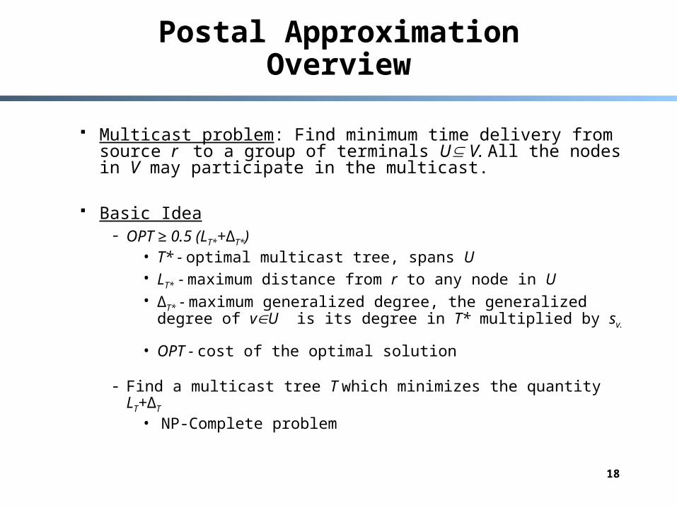
Multicast problem: Find minimum time delivery from source r to a group of terminals U V. All the nodes in V may participate in the multicast.
Basic Idea- OPT ≥ 0.5 (LT*+∆T*)
• T* - optimal multicast tree, spans U• LT* - maximum distance from r to any node in U• ∆T* - maximum generalized degree, the generalized degree of
vU is its degree in T* multiplied by sv.
• OPT - cost of the optimal solution
- Find a multicast tree T which minimizes the quantity LT+∆T
• NP-Complete problem
19
Postal Approximation
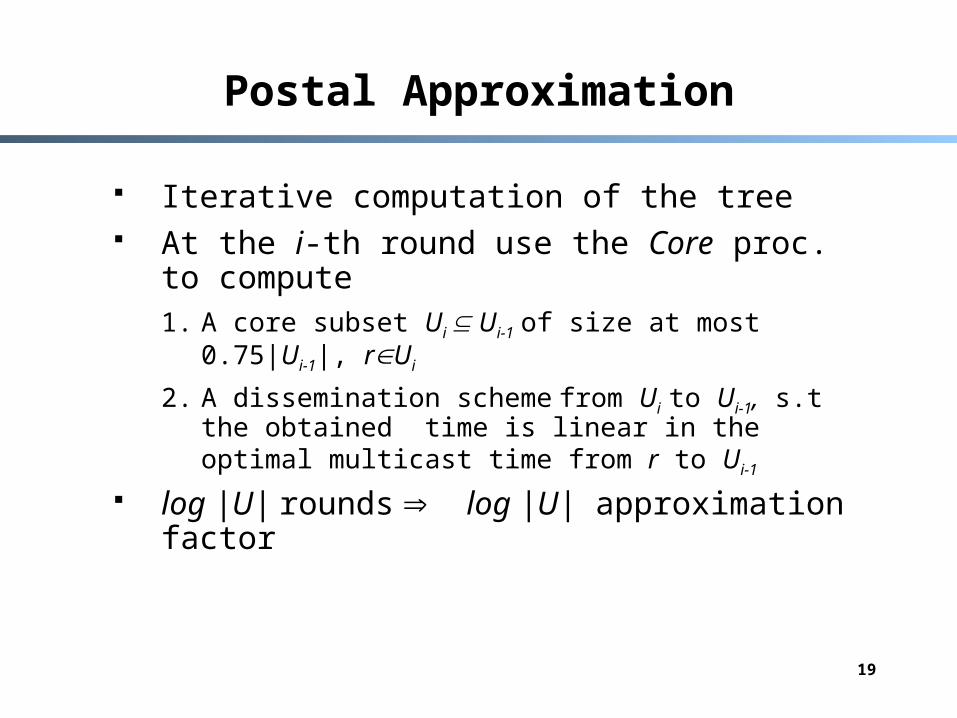
Iterative computation of the tree At the i-th round use the Core proc. to compute
1. A core subset Ui Ui-1 of size at most 0.75|Ui-1|, rUi
2. A dissemination scheme from Ui to Ui-1, s.t the obtained time is linear in the optimal multicast time from r to Ui-1
log |U| rounds log |U| approximation factor
20
Core(U’) Procedure
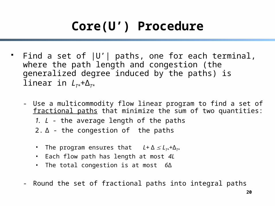
Find a set of |U’| paths, one for each terminal, where the path length and congestion (the generalized degree induced by the paths) is linear in LT*+∆T*
- Use a multicommodity flow linear program to find a set of fractional paths that minimize the sum of two quantities:
1. L - the average length of the paths
2. ∆ - the congestion of the paths
• The program ensures that L+ ∆ LT*+∆T*
• Each flow path has length at most 4L
• The total congestion is at most 6∆
- Round the set of fractional paths into integral paths
21
Core(U’) Procedure-Cont.
Transform the set of paths into a set of spider graphs
- Each spider contains two nodes from U’
- The spiders span at least half of the nodes in U’
- The diameter and generalized degree of each spider is linear in LT*+∆T*
Include in the core an arbitrary node vU’ from each spider and all the nodes not contained in any spider.
22
GHP Adaptation
GHP support requires modification to the rounding mechanism only
Rounding Theorem [KLRTVV87]- Given a real matrix A, real vectors b,y, s.t Ay=b, a real value t ≥0 s.t
in every column of A
• The sum of all positive entries t
• The sum of all negative entries ≥ -t
Then, we can compute an integer vector y, s.t for every i
tbbbyAyyyy iiiiii where, and or
23
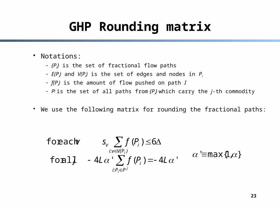
GHP Rounding matrix
Notations: - {Pi} is the set of fractional flow paths
- E(Pi) and V(Pi) is the set of edges and nodes in Pi
- f(Pi) is the amount of flow pushed on path I
- Pj is the set of all paths from {Pi} which carry the j-th commodity
We use the following matrix for rounding the fractional paths:
},1max{' '4)('4 allfor
6)(each for
ji
i
Pi:Pi
)V(Pi:viv
LPfLj
Pfsv
24
GHP Rounding matrix-Cont.
The sum of the positive entries is at most 4Lα’ The sum of the negative entries is at most -4Lα’
Applying the rounding theorem, we get a set of integer paths s.t the length of each path 4Lα’, and the congestion 4Lα’+6∆
Therefore, the length and the congestion are linear in (LT*+∆T*) α’
25
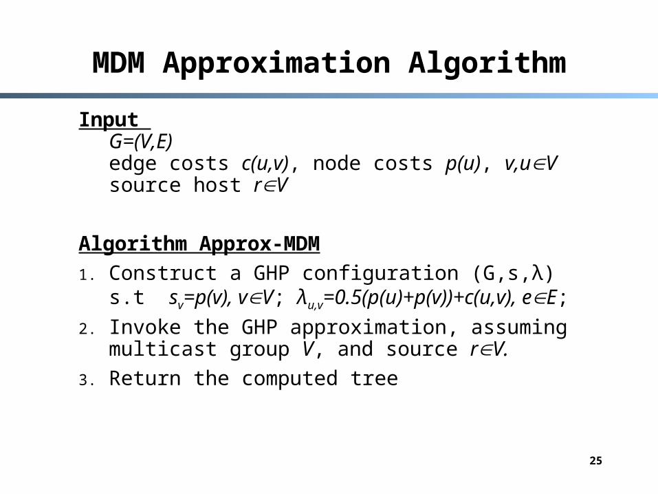
MDM Approximation Algorithm
Input G=(V,E)edge costs c(u,v), node costs p(u), v,uV source host rV
Algorithm Approx-MDM
1. Construct a GHP configuration (G,s,λ) s.t sv=p(v), vV; λu,v=0.5(p(u)+p(v))+c(u,v), eE;
2. Invoke the GHP approximation, assuming multicast group V, and source rV.
3. Return the computed tree
26
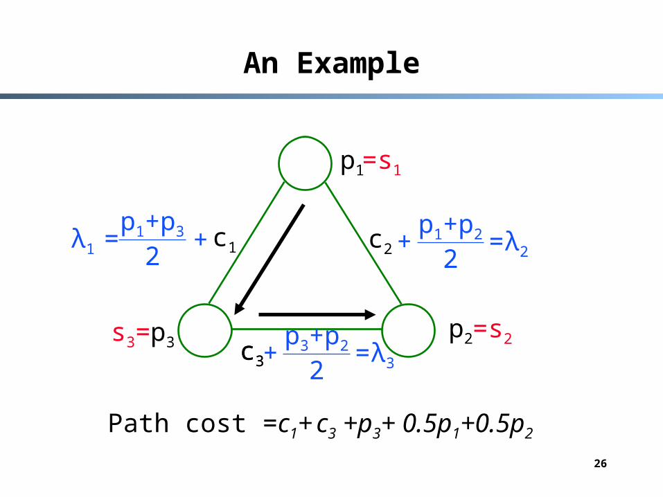
An Example
p1
p3p2
c1 c2
c3
=s1
=s2s3=
p1+p2
2+ =λ2
p1+p3
2+λ1 =
p3+p2
2+ =λ3
c3
Path cost =c1+ c3 +p3+ 0.5p1+0.5p2

27
Approximation Ratio
Theorem 1:
The approximation ratio of Approx-MDM is
(OPT+pmax-pmin) O(log n)
Corollary: The approximation ratio for an overlay network withhomogenous processing costs p(v)=p, vV
OPT • O(log n)
Maximal processing cost
Minimal processing cost
Cost of optimal tree
28
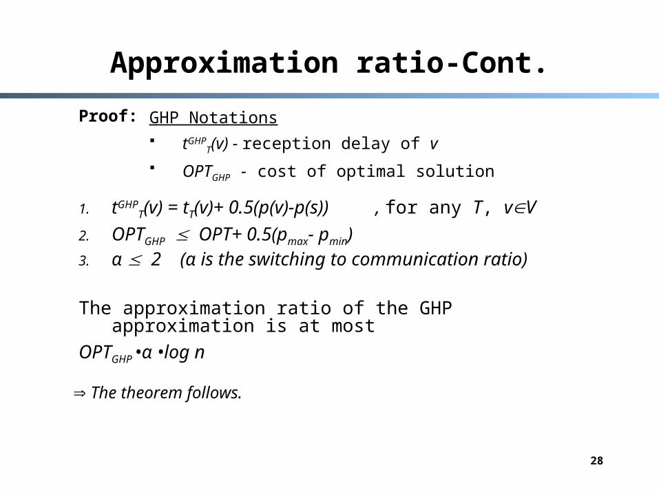
Approximation ratio-Cont.
Proof:
1. tGHPT(v) = tT(v)+ 0.5(p(v)-p(s)) , for any T, vV
2. OPTGHP OPT+ 0.5(pmax- pmin)3. α 2 (α is the switching to communication ratio)
The approximation ratio of the GHP approximation is at most
OPTGHP •α •log n
The theorem follows.
GHP Notations tGHP
T(v) - reception delay of v OPTGHP - cost of optimal solution
29
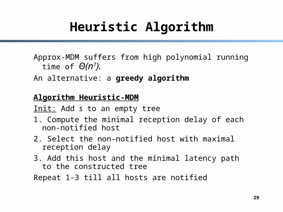
Heuristic Algorithm
Approx-MDM suffers from high polynomial running time of Θ(n7).
An alternative: a greedy algorithm
Algorithm Heuristic-MDM
Init: Add s to an empty tree
1. Compute the minimal reception delay of each non-notified host
2. Select the non-notified host with maximal reception delay
3. Add this host and the minimal latency path to the constructed tree
Repeat 1-3 till all hosts are notified
30
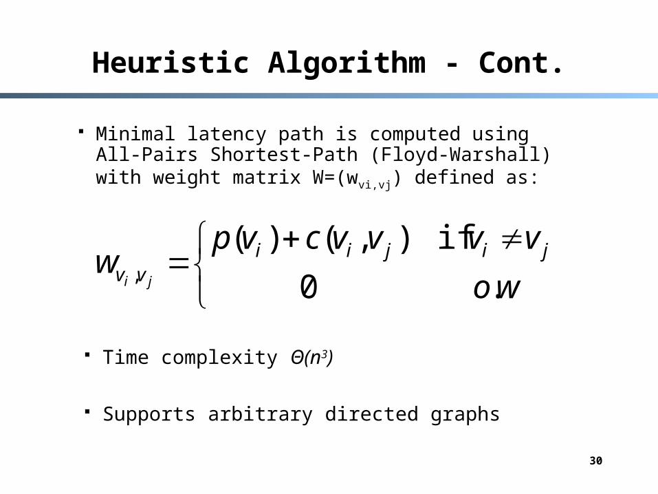
Heuristic Algorithm - Cont.
Minimal latency path is computed using All-Pairs Shortest-Path (Floyd-Warshall) with weight matrix W=(wvi,vj) defined as:
wo
vvvvcvpw jijii
vv ji .0
if),()(,
Time complexity Θ(n3)
Supports arbitrary directed graphs
31
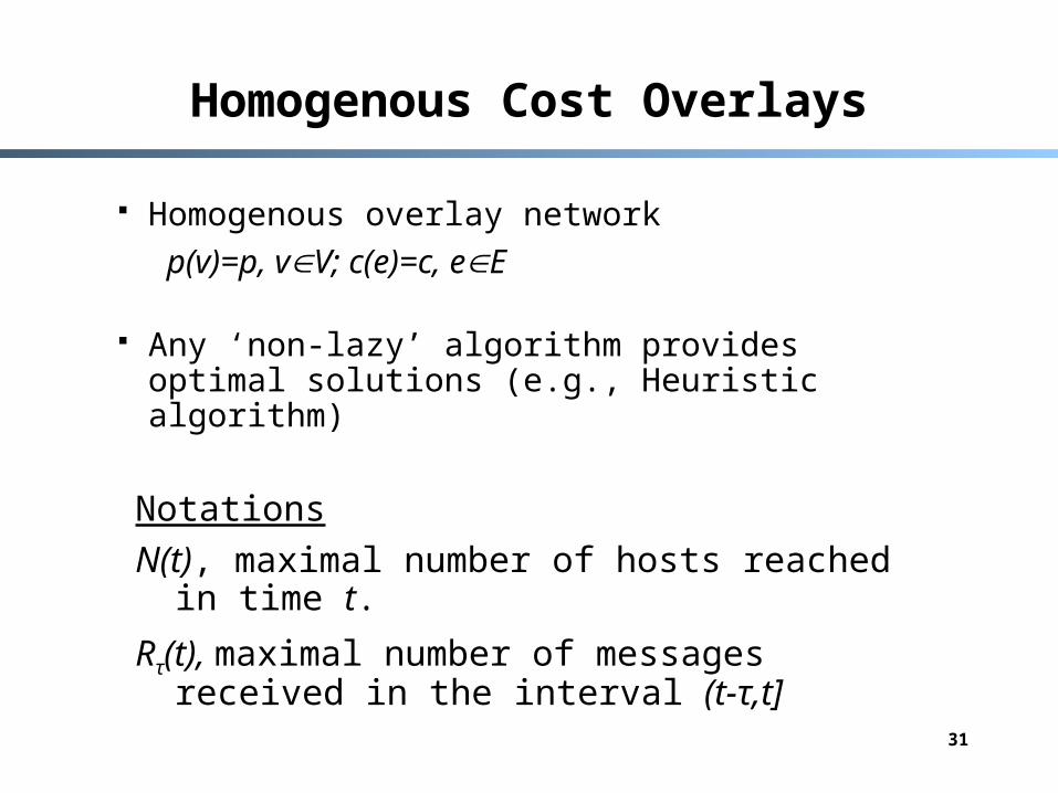
Homogenous Cost Overlays
Homogenous overlay network
p(v)=p, vV; c(e)=c, eE
Any ‘non-lazy’ algorithm provides optimal solutions (e.g., Heuristic algorithm)
Notations
N(t), maximal number of hosts reached in time t.
Rτ(t), maximal number of messages received in the interval (t-τ,t]
32
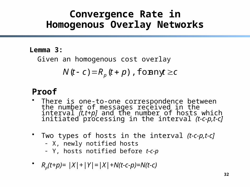
Convergence Rate inHomogenous Overlay Networks
Lemma 3:Given an homogenous cost overlay
Proof There is one-to-one correspondence between the number
of messages received in the interval (t,t+p] and the number of hosts which initiated processing in the interval (t-c-p,t-c]
Two types of hosts in the interval (t-c-p,t-c] - X, newly notified hosts- Y, hosts notified before t-c-p
Rp(t+p)= |X|+|Y|=|X|+N(t-c-p)=N(t-c)
ctptRctN p any for ),()(
33
Convergence Rate inHomogenous Overlay Networks
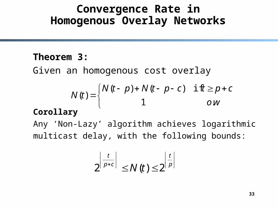
Theorem 3:
Given an homogenous cost overlay
wo
cptcptNptNtN
.1
if)()()(
Corollary
Any ‘Non-Lazy’ algorithm achieves logarithmic
multicast delay, with the following bounds:
p
t
cp
t
tN 2)(2
34
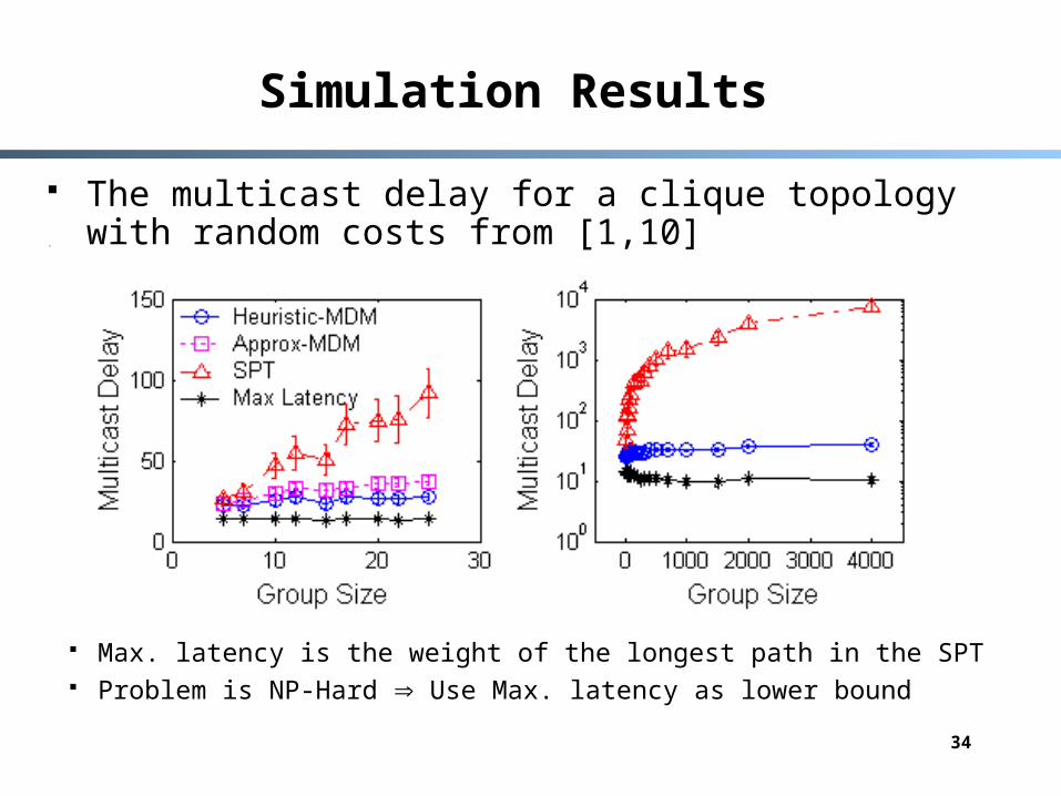
Simulation Results
The multicast delay for a clique topology with random costs from [1,10]
Max. latency is the weight of the longest path in the SPT Problem is NP-Hard Use Max. latency as lower bound
35
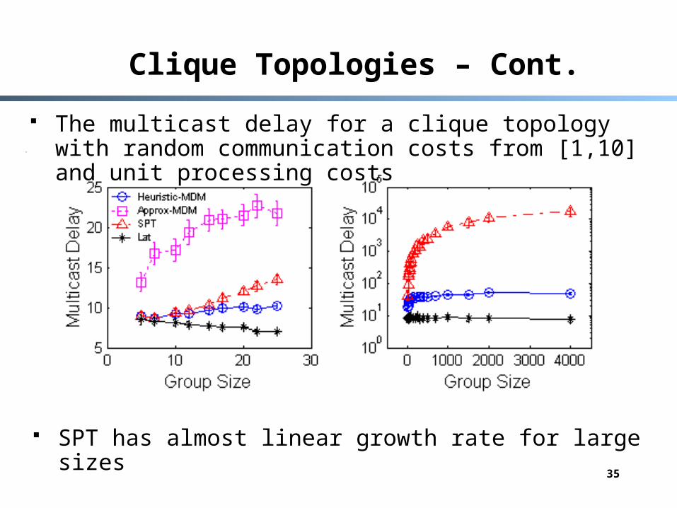
Clique Topologies – Cont.
The multicast delay for a clique topology with random communication costs from [1,10] and unit processing costs
SPT has almost linear growth rate for large sizes

36
Power-Law Topologies
The multicast delay assuming random costs from [1,10]
Simulation based on power-law graphs (Notre-Dame Model [AB00]), average degree is 4.38.
37
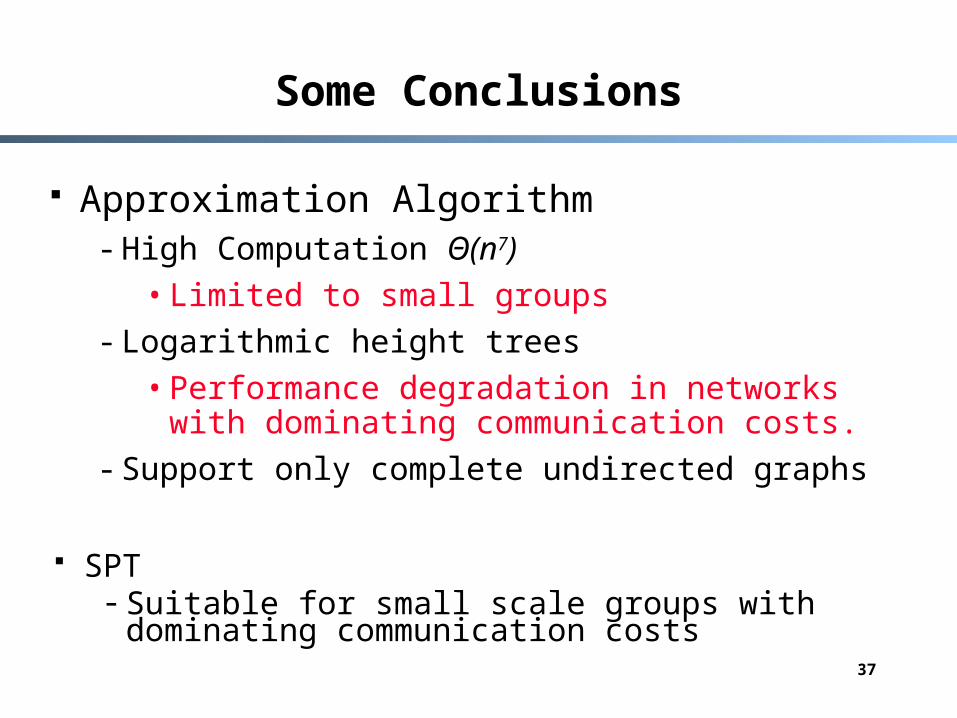
Some Conclusions
Approximation Algorithm- High Computation Θ(n7)
• Limited to small groups
- Logarithmic height trees
• Performance degradation in networks with dominating communication costs.
- Support only complete undirected graphs
SPT - Suitable for small scale groups with dominating
communication costs
38
Simulations Summary
On average the heuristic algorithm has a similar or better performance than the approximation algorithm
Heuristic trees are scalable for large group sizes
- Near optimal result
- Logarithmic like growth rate
39
Remarks
We can reduce the approximation ratio of the Approx-MDM algorithm to a pure logarithmic factor
Graphs in which the triangle equality holds may have better bounds


