Application Note 168 - ARM...

Application Note 168Tracing with RVD

Released on: December, 2006

Copyright © 2006. All rights reserved.DAI0168B

Application Note 168

Application Note 168Tracing with RVD

Copyright © 2006. All rights reserved.

Release Information

The following changes have been made to this application note.

Proprietary Notice

Words and logos marked with ® and ™ are registered trademarks owned by ARM Limited, except as otherwise stated below in this proprietary notice. Other brands and names mentioned herein may be the trademarks of their respective owners.

Neither the whole nor any part of the information contained in, or the product described in, this document may be adapted or reproduced in any material form except with the prior written permission of the copyright holder.

The product described in this document is subject to continuous developments and improvements. All particulars of the product and its use contained in this document are given by ARM in good faith. However, all warranties implied or expressed, including but not limited to implied warranties of merchantability, or fitness for purpose, are excluded.

This document is intended only to assist the reader in the use of the product. ARM Limited shall not be liable for any loss or damage arising from the use of any information in this document, or any error or omission in such information, or any incorrect use of the product.

Confidentiality Status

This document is Non-Confidential. The right to use, copy and disclose this document may be subject to license restrictions in accordance with the terms of the agreement entered into by ARM and the party that ARM delivered this document to.

Product Status

The information in this document is final, that is for a developed product.

Web Address

http://www.arm.com

Table 1 Change history

Date Issue Change

September 2006 A First release

December 2006 B Update example for scatterloading and RVD v3.0.1

2 Copyright © 2006. All rights reserved. DAI0168B


1 Introduction

1.1 Scope

Trace is a powerful debug tool supported by ARM cores that have an Embedded Trace Macrocell (ETM). Trace provides a capture of program instruction flow and data accesses, without impacting the real-time performance of an application. For this reason, trace is an invaluable tool when traditional halted debug methods can not be used for resolving real-time application issues.

This Application Note provides an introduction to tracing with ARM's RealView Debugger (RVD). RVD provides a powerful front end for configuring trace and displaying the results of a trace capture. Since only a limited amount of information can be collected from trace, it is important that your trace capture is properly set to isolate the area of interest for debugging or profiling. This Application Note will focus on the mechanics of performing trace capture using auto trace, trace points, trace ranges and triggers.

A sample application is used as an example throughout the Application Note. This example provides a framework for a series of trace scenarios which can be followed along as a tutorial or used as a reference to make a similar trace capture in your own application.

1.2 Assumptions

This Application Note is written for ETM-enabled targets interfaced to RVD through RealView ICE using an Embedded Trace Buffer or RealView Trace (RVT). Some of the trace scenarios will work on the RealView Instruction Set Simulator (RVISS), but tracing RVISS targets is notably different as defined in the RVD Trace User Guide. A working knowledge of RVD and RVT is assumed.

1.3 References

You may find the following references useful when reading the Application Note:

• Embedded Trace Macrocell Architecture Specification - ARM IHI 0014

• RVDS 2.2 RVD / RVT Tutorial

• RealView Debugger Command Line Reference Guide - ARM DUI 0175

• RealView Debugger Essentials Guide - ARM DUI 0181

• RealView Debugger Trace User Guide - ARM DUI 0322

• RealView Debugger User Guide - ARM DUI 0153

• RealView ICE and RealView Trace User Guide - ARM DUI 0155.

DAI0168B Copyright © 2006. All rights reserved. 3


2 Sample Application

The sample application is supplied in the file TRACE.C. It simulates a small system that reads a set of input data samples, computes the sample average and then outputs the average followed by a variable number of input data samples. It yields code that is easy to follow and provides a framework for common instruction and data trace scenarios.

The application is designed to run on any hardware platform because it simulates data input and output rather than relying on specific peripherals. Data sampling and processing is initiated on a random time basis using the rand() function. Instead of reading data from an input device (such as an analog-to-digital converter), new input data is generated from previous input data. The sample average and input samples are output by writing to a fixed address in memory (intended to simulate the write buffer of a serial port).

The batch file BUILD.BAT is supplied to build the application using RealView Development Suite. The batch file compiles TRACE.C and links the application using the scatterloading file TRACE.SCAT. The scatterloading file places the executable image at 0x8000, followed by the RW and ZI data sections. The application uses a one-region memory model, with the heap and stack placed 256 bytes after the ZI section. The simulated write buffer is located in a separate section at address 0x20000. To run the application from a different address or relocate any of the memory sections, you must modify the TRACE.SCAT file accordingly.

Note 1) The sample application was built using RealView Development Suite v3.0 SP1. If you build the application using a different version of the tools, you may collect slightly different trace captures from those presented in Sections 4 - 8. Any difference in trace captures can be attributed to the difference in assembly code generated by the compiler.

2) The application must be run on RVD with semihosting enabled because it contains calls to printf().

3) The application control loop contains a call to printf() which provides feedback on program execution. Standard semihosting places the target in a debug state which slows program execution and impacts trace profiling results. You can comment out the call to printf() and rebuild the progam to make the program execute faster. If you comment out the call to printf(), your trace captures may no longer match those in Sections 4 - 8.



3 Configuring Trace

3.1 Trace Interfaces

Trace can be collected only from ARM cores that feature an Embedded Trace Macrocell (ETM). The ETM generates trace information based on your trace settings. Trace information output by the ETM must first be stored so that it may be sent to RVD for analysis. The ETM allows two different interfaces for collecting trace data - a dedicated trace port and external buffer or an on-chip Embedded Trace Buffer.

Collecting Trace from an External Trace Port using RVI/RVT

If your target utilizes a trace port, trace data is collected by RealView Trace (RVT). RVT sits on top of RealView ICE (RVI) and the two are connected through a 60-pin and 80-pin connector. RVT interfaces to the trace port through a 38-pin Mictor connector. When a trace capture is made, the ETM fills the contents of RVT memory with trace data through the trace port. The trace data is then uploaded to RVD for analysis via RVI:

Figure 1

Note This is the default configuration expected by RVD.

Collecting Trace from an ETB using RVI

If your ETM features an Embedded Trace Buffer (ETB), then you don't need a trace port or RealView Trace to make a trace capture. Instead, the ETB collects trace information and sends it to RVD through the JTAG port via RVI:



Figure 2

Note The trace interface is implementation defined. It will either be a 38-pin Mictor connector or JTAG interface. Some designs may provide both interfaces. You must configure the tools to use an ETB since they default to using an external trace port.

If your target does feature an ETB, you will see it when you configure the RVI scan chain from the Connection Control window in RVD. The ETB will be identified as "ETMBUF" by the RVI configuration utility:

Figure 3

If you want to trace using ETB, you must enable this option by selecting your ARM core in the scan chain and clicking "Device Properties":



Figure 4

Click the checkbox for the Embedded Trace Buffer and select OK:

Figure 5

The RV Configuration utility will now show that the ETB will be used for tracing:



Figure 6

3.2 Enabling and Configuring Trace

Trace is enabled and configured through RVD. Before you can configure trace, trace must first be enabled from the "Tools - Analyzer/Trace Control - Connect Analyzer/Analysis" menu.



Figure 7

After you enable trace, a message will be displayed indicating which ARM core and ETM you have connected to:

Figure 8

If you receive an error when enabling trace, verify that your target does have an ETM and that it is supported by your version of RVI firmware. If you are tracing with RVT, check that RealView ICE (RVI) and RVT are properly connected and RVT is connected to your target through the 38-pin Mictor connector. If you are tracing with an Embedded Trace Buffer (ETB), check that you have properly enabled ETB trace from the RVI Configuration Utility as described in Section 3.1.

Once trace is enabled, you can configure it from the "Tools - Analyzer/Trace Control - Configure Analyzer Properties" menu. The options available in the ETM Configuration dialogue depend upon your ETM architecture version and the features it has enabled. You can expect some dialogue options to be unavailable for selection (i.e., grayed out). A sample configuration dialogue for the ETM v3.1 architecture is shown below.



Figure 9

The remainder of this Application Note assumes that trace is properly enabled and the ETM is properly configured. Consult the Technical Reference Manual for your specific ETM and the RVD Trace User Guide for guidelines on configuring the ETM.

3.3 Reducing the Trace Buffer Size

RVD sets the default trace buffer size for RVT to the maximum (4,194,304). This results in a tremendous amount of trace information that can take RVD several seconds to process and display. If you prefer to capture less data and have it displayed more quickly, you can adjust the trace buffer size using the "Edit - Set Trace Buffer Size" menu from the Analysis window:



Figure 10

Valid trace buffer sizes are 16,384 to 4,194,304. If you are using an ETB, the trace buffer size is based on the design of your target's ETM and it can not be modified.

Figure 11

Note A trace buffer size of 1,000,000 should be sufficient to replicate the trace captures in Sections 4 - 8.

3.4 Target Specific Information

The trace captures presented in this Application Note were made using an ARM1136JF-S Core Module with RVD v3.0. This target features an ETM11RV which is based on ETM Architecture v3.1. Trace captures made from ETM v1.x architectures will appear different in RVD v3.0:

• For v1.x ETMs, the Elem (element) column starts with "-N" and decrements to the last element "0". The element number may not always decrement by one. The decrement factor depends on the contents of each trace packet and the trace buffer packing setting. For v3.x ETMs, the element column starts with 0 and increments sequentially to "N".



• For v1.x ETMs, the Time/cycle column of the Analysis window is unpopulated if Cycle Accurate trace or Timestamping is not enabled. For v3.x ETMs, the Time/cycle column provides an instruction count if Cycle Accurate trace or Timestamping is not enabled.

The following captures, from an ARM926 (ETM v1.3) and ARM1136 (ETM v3.1) respectively, demonstrate these differences:

Trace from ARM926EJ-S:

Figure 12

Trace from ARM1136JF-S:

Figure 13



4 Auto Tracing

After trace is enabled and configured as described in Section 3, RVD places your target in an Auto Tracing mode by default. This means that if you run and halt your program, instruction trace will automatically be captured.

4.1 Tracing from Program Entry

To observe how Auto Tracing works, load TRACE.AXF to your target. Place a breakpoint at the call to Init() from main(), as shown below.

Figure 14

Run to the breakpoint. When the breakpoint is reached, program execution is stopped and the contents of the trace buffer are sent to RVD for display.

A trace capture is viewed in the Trace Analysis window. The Trace Analysis window can be opened from the "View - Analysis Window" menu. This option is only available when trace is enabled.

Open the Trace Analysis and observe your Auto Tracing capture. You should see that tracing begins from your program entry point, 0x8000 if built with the supplied files.



Figure 15

The trace capture contains the application initialization performed by the C library. If you examine the program's assembly code from the "Dsm" source tab in RVD and scroll to the end of the trace buffer, you will see that tracing ends with the instruction immediately preceding the call to Init() in main(). This instruction is highlighted in red below.

Figure 16

4.2 Tracing to Another Breakpoint

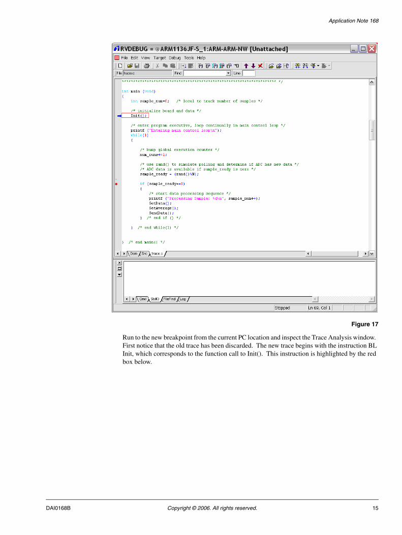
As a follow on to the capture made in Section 4.1, remove the breakpoint at the call to Init() and place another breakpoint in the while(1) loop at the instruction if (sample_ready == 0), as shown below.



Figure 17

Run to the new breakpoint from the current PC location and inspect the Trace Analysis window. First notice that the old trace has been discarded. The new trace begins with the instruction BL Init, which corresponds to the function call to Init(). This instruction is highlighted by the red box below.



Figure 18

The Analysis window supports source code tracking to help you follow the execution of your program. Highlight a sample from Init(), such as trace Element 10 shown below.

Figure 19

Now click on the Source tab in the Analysis window and observe the effects of source code tracking. Namely, line 117 in the source file TRACE.C is now highlighted. This line of C code corresponds to the highlighted element from the Trace tab. Now highlight another line from the Source tab and toggle back to the Trace tab. Observe that source code tracking can be used from both tabs.



Figure 20

Note Source code tracking from the Analysis window also causes source code tracking to occur in the RVD code window. You can bring the PC back into focus by right-clicking in the RVD code window and selecting "Scope to PC". This has no effect on the Analysis window.

If you scroll through the entire trace buffer, you will see that over 3000 samples are captured. Most of these are attributed to the printf() for printing the message "Entering main control loop". The ARM libraries are supplied only in object form. If you try and view the source code of traced library code, you will see the message "no source available" in the Analysis window.



5 Trace Start and Stop Points

Trace Start and Stop points are used to define points in your code where tracing will start and stop. They are most useful for reducing the amount of trace which can be generated from Auto Tracing and they allow one to focus on specific areas of program execution.

5.1 Using a Trace Start Point

Trace Start points are used to initiate trace capture and do not require a matching Trace Stop point. For instance, to bypass the capture of the application startup code, you could place a Trace Start point at the call to Init() and use a breakpoint to end the trace capture.

Place the cursor in the left gutter of the Init() line in the source window, click the left or right mouse button and select Set/Toggle Tracepoint as shown below.

Figure 21

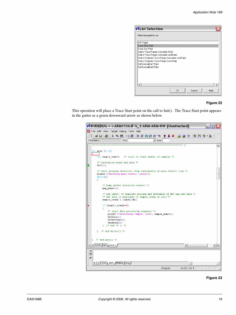
From the List Selection dialogue, select "Trace Start Point" and click "OK" as shown below.



Figure 22

This operation will place a Trace Start point on the call to Init(). The Trace Start point appears in the gutter as a green downward arrow as shown below.

Figure 23



Reload the image using the "Target - Reload Image to Target" menu. Observe that reloading the image from this menu retains your breakpoint and tracepoint. This reload operation will be used throughout the Application Note.

Run to the breakpoint. Notice that the trace capture is the same trace as that from Section 4.2. Namely, the application startup code is not traced, and tracing begins with the BL Init instruction at address 0x8238.

There is one minor difference in the captures. This capture begins with "Warning: Trace pause" to indicate that the target was running when trace became activated from executing the Trace Start point. The capture made with Auto Tracing in Section 4.2 starts with "Warning: Debug state" to indicate that the target was in debug mode (halted) just before tracing began.

Figure 24

5.2 Using Trace Start/Stop Points to Time Function Execution

A Trace Start and Trace Stop point pair can be used to determine the execution time of a function. To obtain timing information from trace, either Cycle Accurate trace or Timestamping must be enabled. These selections are made from the ETM Configuration dialogue. By default both options are disabled.



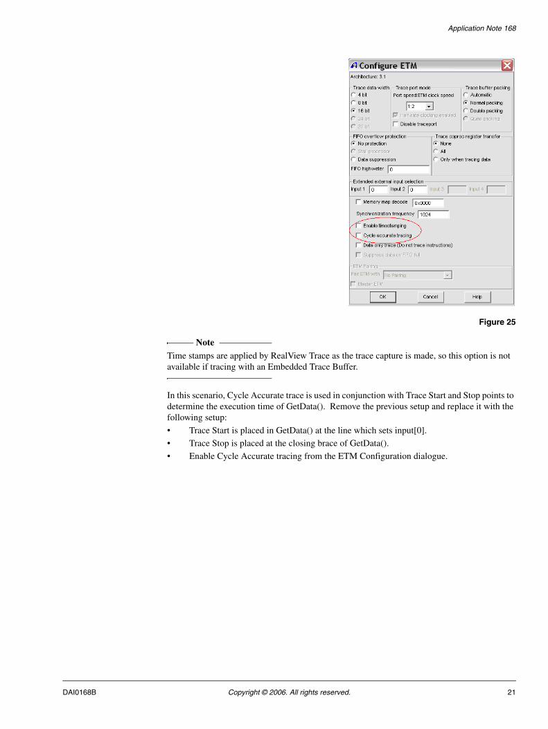
Figure 25

Note Time stamps are applied by RealView Trace as the trace capture is made, so this option is not available if tracing with an Embedded Trace Buffer.

In this scenario, Cycle Accurate trace is used in conjunction with Trace Start and Stop points to determine the execution time of GetData(). Remove the previous setup and replace it with the following setup:

• Trace Start is placed in GetData() at the line which sets input[0].

• Trace Stop is placed at the closing brace of GetData().

• Enable Cycle Accurate tracing from the ETM Configuration dialogue.



Figure 26

The Disassembly source view (from the Dsm tab) of GetData() and the trace points are shown below.



Figure 27

Reload the program using the "Target - Reload Image to Target" menu such that your trace points are retained. Run the program for a few seconds and then stop it. Observe the program output in the RVD StdIO output window:

Figure 28

Open the Trace Analysis window, scroll through the trace capture and observe the following:

• Only instructions from GetData() are traced.

• A continuous trace segment begins with the LDR instruction at 0x8144 and ends with the BLT instruction at 0x81A0.

• Just before trace is paused, the final BLT instruction is not executed and is marked "NoExec" in the Type column.

• The BX LR instruction which returns from GetData() is not traced due to the placement of the Trace Stop point (see the previous Dsm source view).



• Trace discontinuities are marked by "Warning: Trace Pause". This message represents the execution between the exit of GetData() and the entry of GetData() when trace is not captured.

• After the trace pause, tracing always starts again from the Trace Start point.

Figure 29

Note The effects of Cycle Accurate trace can be observed in the second trace column, "Time/cycle". By default RVD will display the time in cycles. This column only contains valid timing information if Cycle Accurate trace or Timestamping is enabled.

To determine the execution time of GetData(), highlight the instruction after a trace pause message (this will be the instruction at the Trace Start point):

Figure 30

Without clicking in the Analysis window, scroll down to the next Trace Pause message. Right-click the BLT instruction just above the Trace Pause message and select "Time Measured from Selected…":



Figure 31

RVD will return the time difference between the two trace samples. In this instance, the time difference is the execution time of GetData(). The same measurement can be obtained by manually subtracting the time of element 416 (51,935,185) from the time of element 623 (51,944,976):

Figure 32

Note Execution time is hardware dependent. Your measured execution time for GetData() may be different.

The time unit of the trace elements and the computed time difference can also be displayed in absolute time (i.e., µS). This selection is made from the "View - Scale Time Units" menu from the Analysis Window:



Figure 33

In order to convert cycles to absolute time units you must enter a processor speed from the "View - Define Processor Speed for Scaling…" menu. The default processor speed is 20 MHz. Any changes made to the time units and processor speed take immediate effect on the trace capture.

Figure 34

Set the processor speed to your core speed and perform another time measurement using absolute time. If you are using a 180 MHz clock, the 9791 cycles equate to 54.39 µs.

Figure 35



In your real application, Trace Start and Stop points may be particularly useful if you are interested in timing a function that is interrupted by an interrupt service routine (ISR), because the ISR will also be traced. This allows you to see the occurrence of ISR disruptions and determine the absolute maximum execution time for a function.



6 Trace Ranges

Trace Ranges provide an alternate method to Trace Start / Stop points for controlling the region of your program that is traced. Trace Ranges allow you to define a continuous address range for tracing. If the program counter (PC) resides within the defined address range, trace is captured. If the PC is outside the address range, trace is not captured.

6.1 Comparing a Trace Range with Trace Start / Stop Points

To observe the difference between tracing with Trace Ranges and Start / Stop Points, the while(1) loop of the sample program will be traced using each method.

Tracing while(1) with Trace Ranges

Reload TRACE.AXF and remove all trace points and breakpoints. Using the Disassembly source view, place the trace range:

• Start of Trace Range (Instruction Only) at 0x8244 (on B 0x829C)

• End of Trace Range (Instruction Only) at 0x82A0 (just after B 0x8248)

Figure 36



Run the program for several seconds and stop it. Inspect the Analysis window and note the following:

• Only instructions residing within the address range are traced.

• A "Warning: Trace pause" message is generated every time a function is called from the while(1) loop.

• Most of the trace capture consists of the same four C lines, which call rand() and check the value of sample_ready.

Figure 37

Search through the trace capture using the "Find - Find Address Expression" menu from the Analysis Window. Search for 0x828C, the address of the BL __0printf instruction for printing the "Processing Sample" message:

Figure 38

You will be brought to the next occurrence in the trace buffer where sample_ready equals 0 and processing occurs. Note that the functions __0printf(), GetData(), GetAverage() and SendData() are not actually traced because they lie outside the active trace range. Discontinuities in the trace capture are marked with "Warning: Trace pause".



Figure 39

Tracing while(1) with Trace Start / Stop Points

Reload TRACE.AXF and remove the Trace Range that you set in Section 6.1.1. Using the Disassembly source view, place the Trace Start and Stop points:

• Trace Start at 0x8248 (on LDR r0, 0x830C)

• Trace Stop at 0x829C (on B 0x8248)



Figure 40

Run the program for several seconds and stop it. Inspect the Analysis window and note the following:

• The while(1) loop and all function calls made from while(1) are traced

• The only instruction not traced is the Trace Stop point. This instruction (B 0x8248 located at address 0x829C) is used to return to the top of the while(1) loop

• A "Warning: Trace pause" message is generated when the Trace Stop point is reached.

• After the trace pause message, the first traced instruction is the Trace Start point (LDR r0, 0x830C located at 0x8248).



Figure 41

Note On some ETM v1.x targets, the "Warning: Trace pause" message may not be generated because the instruction located at the trace stop point (at address 0x8274) may also be traced.

Search through the trace capture using the "Find - Find Address Expression" menu from the Analysis Window. Search for 0x828C, the address of the BL __0printf instruction for printing the "Processing Sample" message:

Figure 42

You are brought to the next point in the buffer where sample_ready equals 0 and processing occurs. Note that now the entire __0printf function is traced, unlike the Trace Range capture made in Section 6.1.1:



Figure 43

To confirm that other function calls from the while(1) loop have been traced, search for them by name using the "Find - Find Symbol Name" menu from the Analysis Window. No parenthesis should be used when entering the function name:

Figure 44

The Symbol Name search for GetData will bring you to the next occurrence in the trace buffer of a trace element from GetData():



Figure 45

Now search for the symbols rand, GetAverage and SendData to show that all functions from the while(1) loop are traced.

6.2 Trace Range Exclusions

Trace Range Exclusions are used to prevent trace from being captured over a specified address range. Trace exclusions are particularly useful if you have a function that is frequently called, but you don't want it traced. You may decide to exclude code portions from your trace capture so you can save the limited trace memory for areas that are of greater interest. For instance, trusted library functions may be good candidates for trace exclusion if you require more trace visibility of your own written code.

In this scenario a Trace Start Point is used to enable trace capture, and an Excluded Trace Range is used to prevent the function GetData() from being traced. Remove the previous trace setup. Using the C source view, place the following trace points:

• Trace Start Point in main() at while(1)

• Start Excluded Trace Range (Inst + Data) at start of GetData()

• End Excluded Trace Range (Inst + Data) at end of GetData()

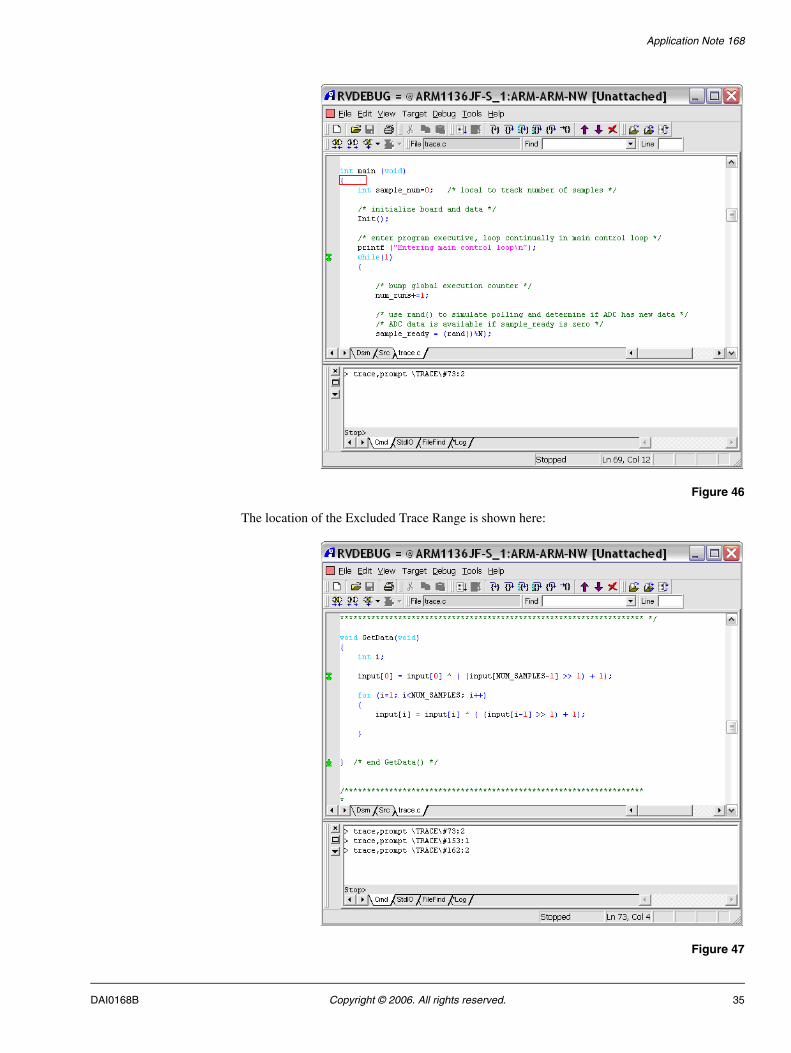
The location of the Trace Start Point is shown here:



Figure 46

The location of the Excluded Trace Range is shown here:

Figure 47



Reload TRACE.AXF, run the program for a few seconds and stop it. Open the Trace Analysis window, scroll through it and observe that the while(1) loop is traced. Perform a search for GetData using the "Find - Find Symbol Name" menu from the Analysis Window:

Figure 48

Observe that there is only one instruction traced from GetData(), while all the other functions called from the while(1) loop are completely traced. The BX LR instruction from GetData() is used to return from the function. It is present in the trace capture because the end of the excluded trace range fell at this address (0x81A4) when the trace range was set from the C source view.

Figure 49

You must be aware that this is a common occurrence when placing trace points from the C source window (from the Src tab). The effects of this phenomenon can be even greater if you build your application with a high level of compiler optimization. Precise control of trace point placement can be achieved using the Disassembly source view.

To exclude all instructions of GetData() from the trace (including the BX LR which was previously traced), the Trace Range Exclusion must be set using the Disassembly source view. Click on the Dsm tab and remove the previous trace range by clicking on either trace range point and selecting "Clear Break":



Figure 50

Note Do not remove the Trace Start Point.

Place the new Excluded Trace Range at address locations 0x8144 (the first instruction in GetData()) and 0x81A8 (the first instruction in Init()):



Figure 51

Reload the program, run it for a few seconds and stop it. Observe that the new trace condition results in a trace capture with all instructions of GetData() removed:

Figure 52

Interestingly, if you run and stop the program again after it is halted, the Trace Analysis window will be empty and report "<No Data in Buffer>" :



Figure 53

Trace data is not captured because the trace conditions have not been met. The Trace Start Point (at the while(1) statement) is only executed once in the program (not every time through the loop). For trace to be collected again, you will have to reload TRACE.AXF so that the Trace Start Point instruction is executed.



7 Tracing Data

Trace is customarily used to determine program execution flow and Sections 4 - 6 of this Application Note have described methods of capturing Instruction Trace. However, there are times when you require visibility of the data accesses made by your program. The Embedded Trace Macrocell (ETM) provides the ability to trace data and this section describes how data trace can be performed from RVD.

Tracing data is a very data intensive operation and may result in trace overflows if you are not tracing with an ETB. Trace overflows occur when the internal FIFO of the ETM is full and new trace data is prevented from being stored. To minimize the possibility of trace overflow, configure your ETM to use the maximum possible trace data width (typically 16 bits) and disable Cycle Accurate trace:

Figure 54

7.1 Tracing Data With Auto Trace

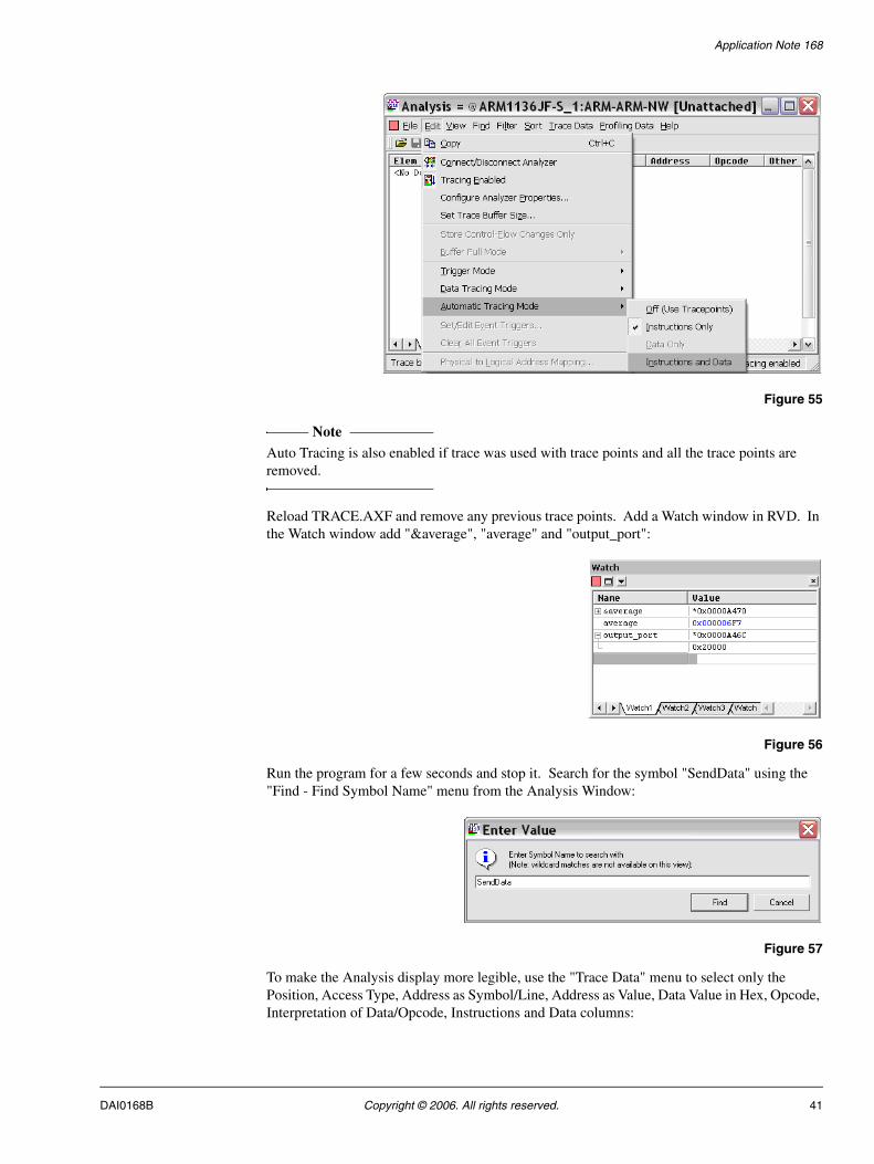
After trace is first enabled and configured as described in Section 3, RVD places your target in Auto Tracing mode. By default, only instructions are traced. To enable Auto Tracing for instructions and data, use the "Edit - Automatic Tracing Mode" menu from the Analysis window and select "Instructions and Data" as shown below:



Figure 55

Note Auto Tracing is also enabled if trace was used with trace points and all the trace points are removed.

Reload TRACE.AXF and remove any previous trace points. Add a Watch window in RVD. In the Watch window add "&average", "average" and "output_port":

Figure 56

Run the program for a few seconds and stop it. Search for the symbol "SendData" using the "Find - Find Symbol Name" menu from the Analysis Window:

Figure 57

To make the Analysis display more legible, use the "Trace Data" menu to select only the Position, Access Type, Address as Symbol/Line, Address as Value, Data Value in Hex, Opcode, Interpretation of Data/Opcode, Instructions and Data columns:



Figure 58

Note The traces in Section 7 are made with Cycle Accurate trace disabled and Timestamping disabled. If you require timing information from your data trace, enable either Cycle Accurate trace or Timestamping as shown in Section 5.2. To view timing information in the Analysis window, select "Absolute Time" or "Relative Time" from the "Trace Data" menu.

Your trace capture should now have the following columns of data:



Figure 59

Note Your capture may have different element numbers and different values in the Data/Hex and Other columns.

In the trace capture observe that the first data access in SendData is at trace element 383. This access is a read from address 0x82D0 of data 0xA470. This read is generated from the execution of the LDR r2, 0x82D0 instruction (boxed in red). This read is for the computation of the local variable "num_xmit", which resides on the stack:

int i, num_xmit;num_xmit = (average & 0xF) + 1;

Trace element 384 contains the next data access and this is a read of the global variable "average". The Watch window shows that "average" is stored at 0xA470. Note how "average" also appears in the Symbolic column. In this particular run, average has a value of 0x5E3.

This segment of the trace capture contains two data write operations at trace elements 390 and 395. These are the respective writes of the packet header (0xAAAAAAAA) and computed average (0x5E3) to address 0x20000 (the address of output_fifo, pointed to by *output_port):

*output_port = HEADER; /* output header packet */*output_port = average; /* output average value */

To further improve the trace display, enable "Instruction Boundaries" from the "Trace Data" menu in the Analysis window. This provides a slightly clearer view for interpreting which instruction performed the data access. This view still includes entries which don't make data accesses, such as elements 385 and 386:



Figure 60

If you want to focus solely on data accesses, you can enable "Function Boundaries", disable "Instruction Boundaries" and disable "Instructions" from the "Trace Data" menu:



Figure 61

This setting provides a clean view of data accesses and still provides some visibility to general program location:



Figure 62

Perform a search for the symbol GetAverage using "Find - Find Symbol Name" from the Analysis Window:

Figure 63

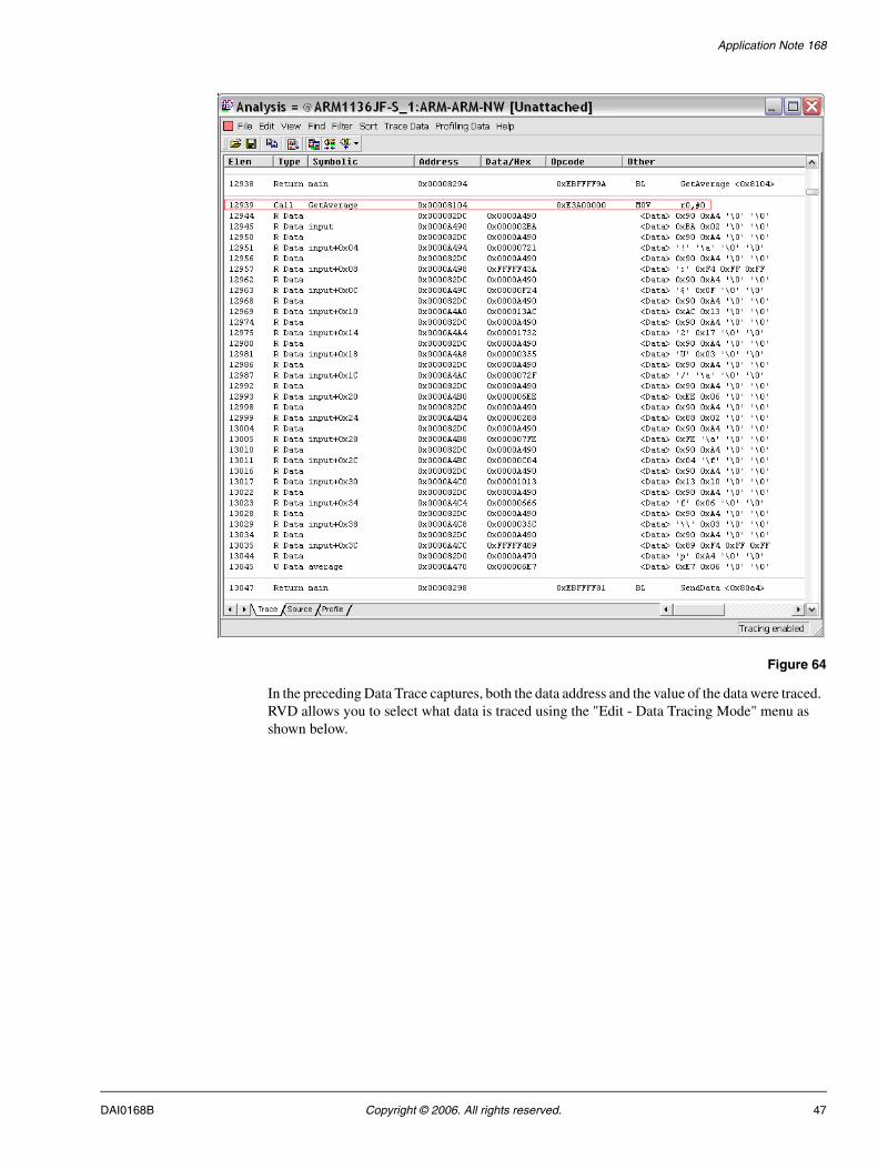
In GetAverage(), observe how the array input[ ] is accessed sequentially to compute "average" and how the array elements are represented in the Symbolic column. The last data operation in the function is a write to "average". In this particular run, the average of array input[ ] is 0x6E7.



Figure 64

In the preceding Data Trace captures, both the data address and the value of the data were traced. RVD allows you to select what data is traced using the "Edit - Data Tracing Mode" menu as shown below.



Figure 65

The default Data Tracing mode is "Data and Address". You can use the "Address Only" and "Data Only" options to reduce the amount of data collected by the ETM, and this will lessen the possibility of trace overflow. If the same capture is made with Data Tracing Mode set to "Address Only", data value information is not traced and the Data / Hex column is empty:



Figure 66

If another capture is made with Data Tracing Mode set to "Data Only", data address information is not traced and the Address column is empty for all data accesses:

Figure 67

7.2 Tracing Data from an Instruction Trace Range

In Section 6 Trace Ranges were used to isolate the region of trace to a specified address range. This same trace operation can be used to also capture data accesses. This type of trace capture is valuable if you need to analyze how a particular segment of code is accessing data memory.

Remove any previous trace points and trace SendData() using the following Trace Range:

• Start of Trace Range (Instruction and Data) at opening brace

• End of Trace Range (Instruction and Data) at closing brace



Figure 68

Reload TRACE.AXF and change the Data Tracing Mode back to "Data and Address" if you modified it in Section 7.1. Run the program for a few seconds and stop it. Open the Analysis window. Enable "Instructions" and "Function Boundaries" and disable "Data" from the "Trace Data" menu and observe that trace is paused between runs of SendData():



Figure 69

Note Your trace capture may differ.

Now enable "Data" and disable "Instructions" from the "Trace Data" menu. Scroll through the buffer and observe that each time SendData() runs there is not a consistent number of words written to output_fifo (address 0x20000):



Figure 70

If you reference TRACE.C, you will find that SendData() transmits a packet header (0xAAAAAAAA), the computed average and a variable number of input samples. The number of input samples written in SendData(), num_xmit, is determined by the computed average:

num_xmit = (average & 0xF) + 1;

You can further isolate accesses to a particular address by applying a post-processing filter. Apply a filter to examine all accesses to 0x20000. To do this, use the "Filter - Filter on Address Expression" menu:



Figure 71

Enter 0x20000 from the Address Expression dialogue:

Figure 72

You can now more readily observe all the accesses to 0x20000. Find a trace element that writes the packet header word, 0xAAAAAAAA. Observe that each packet consists of the header word, the computed average and 1 to 16 input samples (based on the least-significant nibble of the average).



Figure 73

In the trace above, SendData() has run four times:

7.3 Tracing Data Accesses to a Specific Address

In the previous scenario, data trace was captured based on execution from a specified address range. This type of capture is useful for most situations. However, an alternate method of data trace is provided by the ETM based solely on data accesses (not instruction accesses). This allows you to trace specific data accesses made from anywhere in your program. You may find this type of trace useful if you have a global variable that is corrupted by a stray write or if you want to see how frequently a variable is accessed.

In this scenario only accesses to *output_port (address 0x20000) are traced. You can configure this type of capture using a Detailed Trace Point. Delete all previous trace points and reload TRACE.AXF. Click on the left gutter of the Source window and select "Set Detailed Tracepoint".

Table 2

Header Element Average Input Words Written Total Words Written

452 0xFFFFFCD0 1 3

477 0x000001A4 5 7

534 0x000001A1 2 4

567 0x00000303 4 6



Figure 74

The Set/Edit Tracepoint dialogue will open. This allows you to set both simple and detailed trace points:

Figure 75

Use this dialogue to configure an instruction and data trace for all accesses of output_port, the pointer to output_fifo. The top three parameters need to be modified:



Figure 76

Use the circled down selector to open the <Variable list…> menu and browse for "output_port of @trace". When this variable is selected it will appear as "@trace\\output_port" in the dialogue:

Figure 77

Click the "OK" button to save the trace point. Observe that the Cmd tab of the output window displays the command used to set the trace point. If you prefer, you may manually enter trace points using the command line from the Cmd tab of the output window. A full description of the command line interface is provided in the RealView Debugger Command Line Reference Guide.

Figure 78

Trace points can be viewed, modified and cleared using the "View - Break/Tracepoints" menu from RVD. View the trace point you just set to confirm that it is set correctly. Since output_port is a pointer, all accesses to the value of the pointer when the trace point was set (0x20000) will be traced.



Figure 79

Run the program for a few seconds and stop it. Open the Analysis window and configure the view of the trace capture. If you applied a trace filter from Section 7.2, remove the filter using the "Filter - Clear Filtering" menu from the Analysis window. Also enable the Data/Hex and Instruction trace view by selecting "Data Value in Hex" and "Instructions" in the "Trace Data" menu (see Section 7.1).

Now scroll through the trace buffer and observe that only three instructions from SendData() are traced. Trace is paused between each traced instruction. The three instructions are all STR instructions from address 0x80C0 (which writes the packet header), 0x80D4 (which writes the average) and 0x80F0 (which writes the input samples):

Figure 80

This capture was configured to trace all accesses to *output_port. RVD allows one to specify the data access type - either a read or write. In this program only writes are made to *output_port, so the same trace capture can be obtained using a trace point that specifies "Data Write" instead of "Data Access":



Figure 81

The variable "average" is both read and written in the program. To trace only the reads of "average", delete the previous trace point and set the following trace point:

Figure 82

Note To trace accesses to a variable, you must manually precede the symbol name with an ampersand to de-reference the address of the variable. To trace accesses to average, you must select "average @trace" from the variable browser. This will be displayed as "@trace\\average" in the dialogue. You must then manually add the ampersand to the "when" field to create "@trace\\&average".

This results in the following command:

Figure 83

Confirm that the trace point is properly set using "View - Break/Tracepoints" from RVD :

Figure 84



Run the program for a few seconds and stop it, you will see that average is only read from two instructions. It is read both times from SendData: once to compute the number of input samples to output (from address 0x80A8), and a second time so that it may be output (from address 0x80C8). In both cases the value of average will always be the same (0x227 in the highlighted line), but it will vary the next time SendData() executes.

Figure 85

Now modify the trace point to trace data writes to &average:

Figure 86

Run the program for a few seconds (it doesn't have to be re-loaded) and stop it. Observe that &average is only written to at one location in the program (in GetAverage()):



Figure 87

7.4 Tracing Data Accesses to an Address Range

In Section 7.3 data traces are configured to trace accesses to a specific address - either *output_port or &average. The ETM also allows data trace to be configured for an address range. In this scenario, all read accesses to the input[ ] array will be traced. Add the input[ ] array to the Watch window to determine the location of the array in memory. The 16-word array resides from 0xA490 (index 0) through 0xA4CF (index 15):

Figure 88



To trace data reads from a memory range, the command line interface must be used. Reload TRACE.AXF, remove any previous trace points and set the following data trace point using the command window:

> trcdread,hw_out:"Tracepoint Type=Trace Instr and Data" 0xa490..0xa4cf

Figure 89

Figure 90

Now run the program for a few seconds and stop it. Scroll through the Analysis window and observe the following:

• Read accesses to input[ ] are made from GetData(), GetAverage() and SendData(). This is most readily observed by clicking on the "Source" tab in the Analysis window.

• All 16 words of input[ ] are read and traced

• Some instructions that don't access the data trace range are traced



Figure 91

The most interesting item in the capture is that the even some instructions that don't make a data access are traced (such as circled elements 557 - 559). Even though this appears to be a problem with the trace, this behavior is defined in the ETM Architecture Specification. Namely, when a data access is made within the specified data range, trace is activated and stays active until a data access is made outside the range.

The instruction at element 556 performs a read of input[15] and this activates trace. The three circled instructions only perform internal register operations so they are also traced. If you reference the Dsm tab of the main RVD window you will see that the next executed instruction is "LDR r2, 0x82DC" (located at 0x8160). This instruction makes a data access outside the trace range so it is not traced and trace is deactivated (paused).



8 Tracing a Running Target

The trace examples presented in Sections 4 - 7 generate trace displays by halting the running target. When a target is halted with trace enabled, the captured trace buffer stored in RealView Trace or the target's ETB is automatically dumped to RVD for display. There may be times when your target can not be stopped to generate a trace capture because it is controlling hardware which must continue to operate. In these situations you will have to make a trace capture from a running target.

There are two methods to perform a capture with a running target. You can either disable trace or use a trace trigger. Both of these scenarios are described in this section.

8.1 Connecting the Analyzer and Disabling Trace

Remove all trace points and breakpoints that you may have set. Ensure that the trace analyzer is not connected. If the trace analyzer is connected, disconnect it using the "Edit - Connect/Disconnect Analyzer" menu from the Analysis window:

Figure 92

When you disconnect the trace analyzer from the Analysis window, the following message is displayed in the RVD command window:

Figure 93

Additionally, the status bar of the Analysis window indicates that the trace analyzer is not connected. When the trace analyzer is not connected, trace is disabled on the target:



Figure 94

Load TRACE.AXF and run the program. Connect the trace analyzer from the RVD "Tools - Analyzer/Trace Control - Connect Analyzer/Analysis" menu. When the analyzer is first connected, trace is enabled with Auto Tracing (see Section 4). In the status bar, observe that trace is now enabled:

Figure 95

Even though tracing is enabled, no trace data is displayed in RVD until the target is halted, tracing is disabled or a trigger point is reached. When the trace buffer is full, trace continues to be captured by overwriting the oldest trace sample in the buffer.

If you need to change the ETM configuration, you can do this even while the target is running. Use the "Tools - Analyzer/Trace Control - Configure Analyzer Properties" menu as described in Section 3. For configuration changes to take effect, tracing is stopped and restarted while your target continues to run. If you do make a change in the configuration, RVD prompts you to allow the change to occur. If you changed the ETM configuration, click the "Yes" button in the RVD prompt:



Figure 96

With the program running and trace enabled, disable trace capture from the "Edit - Tracing Enabled" menu in the Analysis window. This selection toggles tracing on and off:

Figure 97

Observe that when the selection is made, tracing is disabled, the trace buffer is dumped to RVD and the target continues to run:

Figure 98



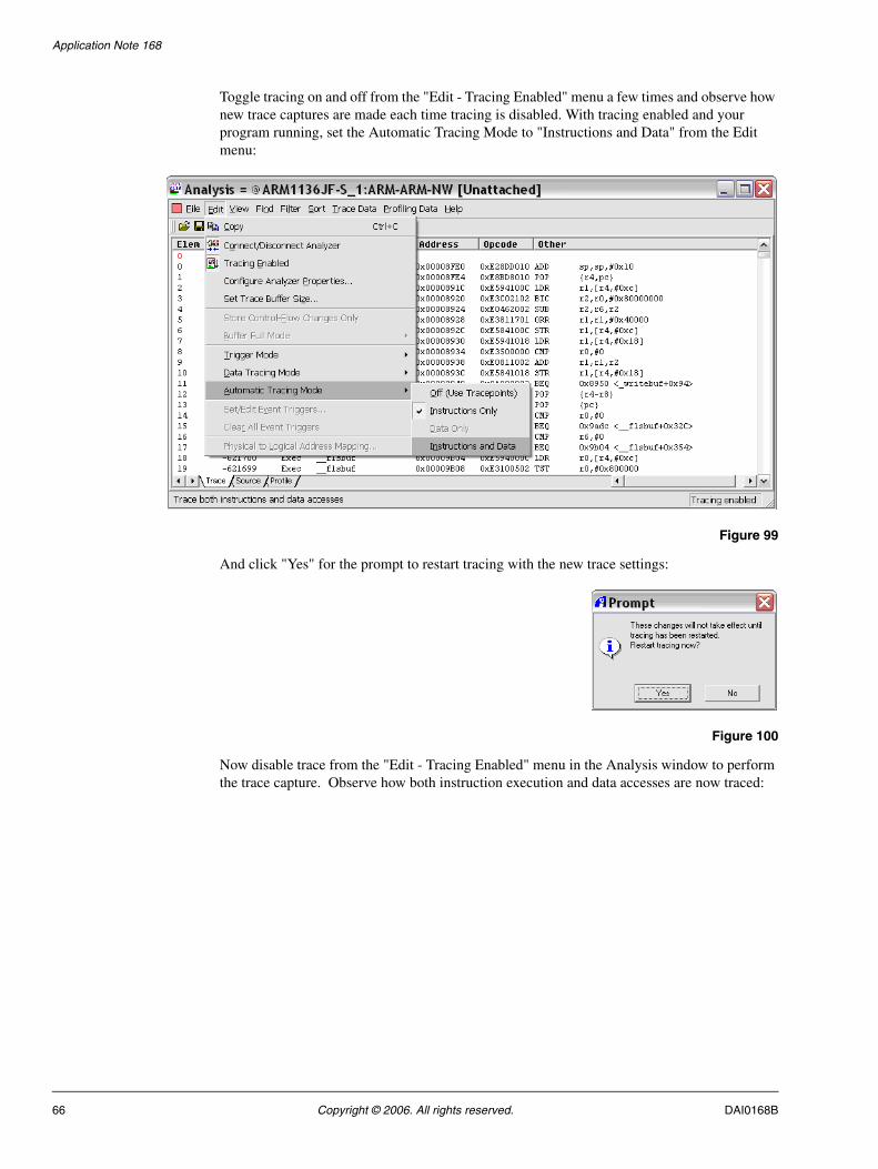
Toggle tracing on and off from the "Edit - Tracing Enabled" menu a few times and observe how new trace captures are made each time tracing is disabled. With tracing enabled and your program running, set the Automatic Tracing Mode to "Instructions and Data" from the Edit menu:

Figure 99

And click "Yes" for the prompt to restart tracing with the new trace settings:

Figure 100

Now disable trace from the "Edit - Tracing Enabled" menu in the Analysis window to perform the trace capture. Observe how both instruction execution and data accesses are now traced:



Figure 101

8.2 Simple Trace Triggers

Triggers are used to initiate a trace capture based upon a user-defined trigger condition. When the trigger condition is met, the target will continue to run and the trace buffer will fill with new data. When the trace buffer is full, the contents of the buffer will be dumped to RVD for analysis. After the trace capture is made, trace is no longer enabled even though your target continues running.

In this scenario a trace capture similar to that from Section 4 will be made with the use of a Trace Trigger instead of Auto Tracing with breakpoints. A trigger will be used to make a trace capture which includes the execution of the C library startup code and entry into the while(1) loop of main().

If you disabled trace in Section 8.1, enable trace as described in Section 3. Set the Automatic Tracing Mode back to "Instructions Only" from the Edit menu in the Analysis Window. Reload TRACE.AXF and remove all trace points. Place a Trigger point at the call to Init() in main():



Figure 102

Open the Trace Analysis window from the "View - Analysis" menu in RVD. Run the program. If you are using RVT, observe that almost immediately the "TRIG" LED lights on the bottom right of the unit. This indicates the trace trigger has been reached. Wait several seconds for the Analysis window to populate with trace data as your program continues to run. Examine the Analysis window and observe that tracing starts from the program entry point (0x8000):



Figure 103

Search for the Trigger in the trace buffer using the "Find - Find Trigger" menu:



Figure 104

Observe that the focus (red letterbox) is brought to the trigger location. The trigger is designated with an asterisk by the Element number:



Figure 105

8.3 Advanced Trace Triggers

For more complex trace situations on running targets, you can use a conditional trigger point. A conditional trigger point allows you to specify the number of times an event (such as instruction execution or data access) must occur for trace to trigger. You can also specify a specific data access as a trigger point, similar to an RVD watchpoint. The exact capability of a conditional trigger point is based on the event resources supported by your ETM.

Using a Pass Counter for Program Execution

In this scenario a trigger is used to capture trace on the 10th execution of SendData(). Remove your previous trigger point and set a simple trace trigger at the computation of num_xmit in SendData():



Figure 106

Reload TRACE.AXF and run it. Wait for the Analysis window to populate with your trace capture. After your trace is displayed, search for SendData using the "Find - Find Symbol Name" menu from the Analysis window:

Figure 107

Observe that the trace trigger is located two instructions after the very first call to SendData() at trace element 9481:



Figure 108

Halt your target. Now display the trigger using the "View - Break/Tracepoints" menu:

Figure 109

Right-click on the trace point and select "Edit Break/Tracepoint". Modify the trace point such that the trigger occurs after the instruction is executed 10 times. Do this is by setting the "Pass" parameter to "10":

Figure 110

Clear the previous trace from the Analysis window using the "View - Clear Trace Buffer" menu. Reload TRACE.AXF and run the program again. Wait for the Analysis window to populate with the new trace capture.

Observe that the new capture starts from the program entry point at 0x8000. Search the buffer again for the trigger point using "Find - Find Trigger". Observe that the trigger is now located at element 63562:



Figure 111

Scroll back to the top of the trace buffer, and search for address 0x8298 using the "Find - Find Address Expression" menu. As shown above, address 0x8298 contains the call to SendData:

Figure 112

Repeat the search 9 times using the "Find - Find Next" menu (or "F3") to confirm that the trigger occurred on the 10th execution of the num_xmit computation. Observe that after the 9 searches you return to trace element 63560.

Note If you are tracing with an ETB, your trace buffer may not be large enough to hold all 10 executions of SendData(). To see the effects of the pass counter, reduce the trigger's pass count accordingly and perform another trace capture.

Using a Pass Counter for Data Accesses

In this scenario a trigger is used to capture the 2000th data write to *output_port. Begin by enabling data trace by setting the Automatic Tracing Mode to "Instructions and Data" as in Section 7.1:



Figure 113

Remove the trigger point set in Section 8.3.1. Set a new trigger point by clicking anywhere in the left gutter and selecting "Set Detailed Tracepoint…":

Figure 114

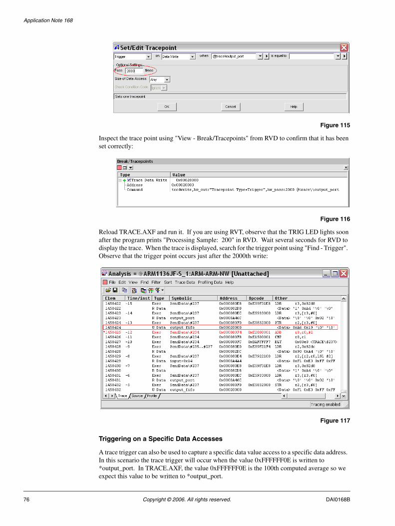
Following the instructions in Section 7.3, set the trigger to activate on the 2000th data write to output_port:



Figure 115

Inspect the trace point using "View - Break/Tracepoints" from RVD to confirm that it has been set correctly:

Figure 116

Reload TRACE.AXF and run it. If you are using RVT, observe that the TRIG LED lights soon after the program prints "Processing Sample: 200" in RVD. Wait several seconds for RVD to display the trace. When the trace is displayed, search for the trigger point using "Find - Trigger". Observe that the trigger point occurs just after the 2000th write:

Figure 117

Triggering on a Specific Data Accesses

A trace trigger can also be used to capture a specific data value access to a specific data address. In this scenario the trace trigger will occur when the value 0xFFFFFF0E is written to *output_port. In TRACE.AXF, the value 0xFFFFFF0E is the 100th computed average so we expect this value to be written to *output_port.



Edit the trigger point set in Section 8.3.2 to activate when the value 0xFFFFFF0E is written to *output_port:

Figure 118

Inspect the trace point using "View - Break/Tracepoints" from RVD to confirm that it has been set correctly:

Figure 119

Reload TRACE.AXF and run it. If you are using RVT, observe that the TRIG LED lights soon after the program prints "Processing Sample: 100" in RVD. Wait several seconds for RVD to display the trace. When the trace is displayed, search for the trigger point using "Find - Trigger". Observe that the trigger point occurs just after the write of 0xFFFFFF0E to address 0x20000 (*output_port):

Figure 120

Scroll up in the trace buffer and observe that in fact 0xFFFFFF0E is the average value computed in GetAverage and written to "average" (located at 0xA470):



Figure 121

Scroll further up the trace buffer and look for another value that is written to *output_port. Modify the trace point to trigger on the data write to *output_port of this new value. Reload TRACE.AXF and repeat the trace capture using the new trigger point. Confirm that the trigger point of the second capture is located at the correct location.


Date post:	17-Jul-2018
Category:	Documents
Upload:	lyque
View:	215 times
Download:	0 times

Application Note 168 - ARM...

Documents