17
Application of a Markov chain traffic model to the Greater Philadelphia Region Joseph Reiter, Villanova University MAT 8435, Fall 2013
| Date post: | 18-Jul-2015 |
| Category: |
Data & Analytics |
| Upload: | joseph-reiter |
| View: | 72 times |
| Download: | 1 times |
Application of a Markov chain traffic model to the Greater Philadelphia RegionJoseph Reiter, Villanova University
MAT 8435, Fall 2013
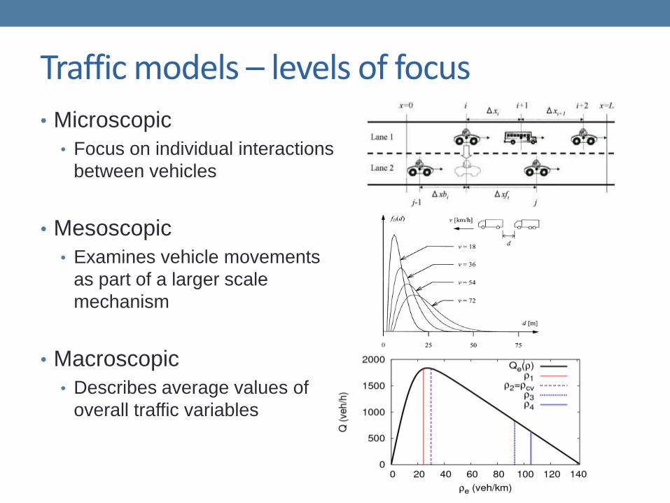
Traffic models – levels of focus
• Microscopic
• Focus on individual interactions
between vehicles
• Mesoscopic
• Examines vehicle movements
as part of a larger scale
mechanism
• Macroscopic
• Describes average values of
overall traffic variables

Representing a highway system as a matrix
• Exits are represented by vertices
and highway segments by edges
• The adjacency matrix for this
graph:
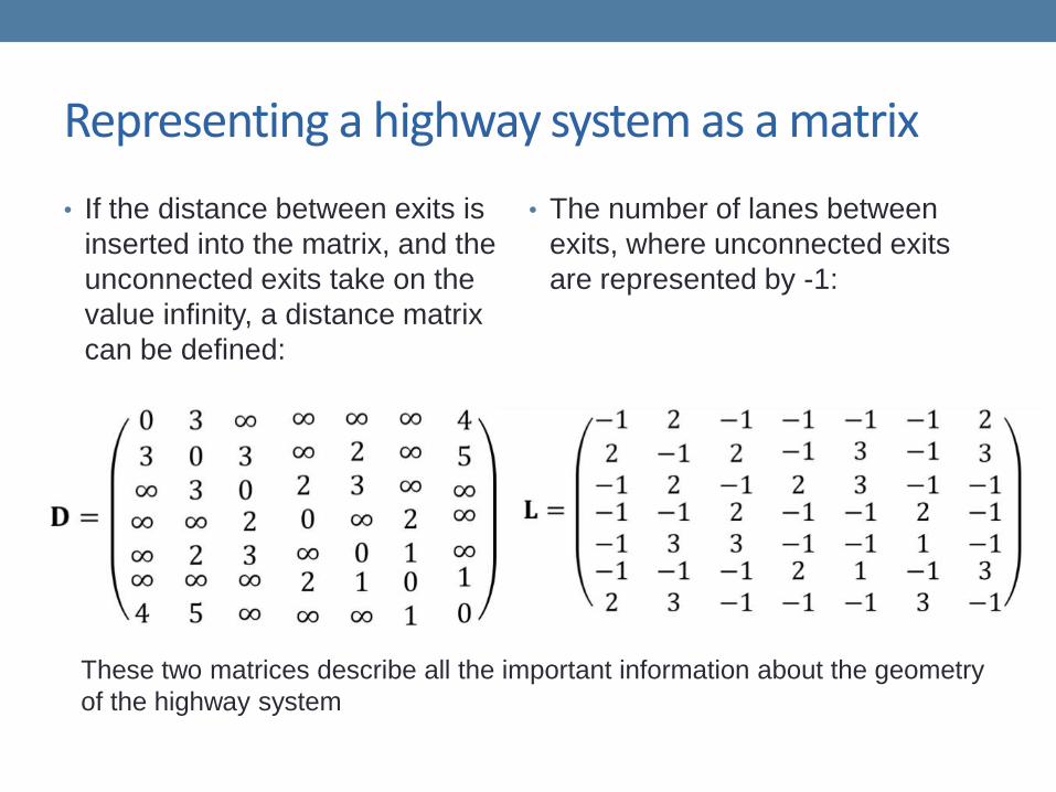
Representing a highway system as a matrix
• If the distance between exits is
inserted into the matrix, and the
unconnected exits take on the
value infinity, a distance matrix
can be defined:
• The number of lanes between
exits, where unconnected exits
are represented by -1:
These two matrices describe all the important information about the geometry
of the highway system
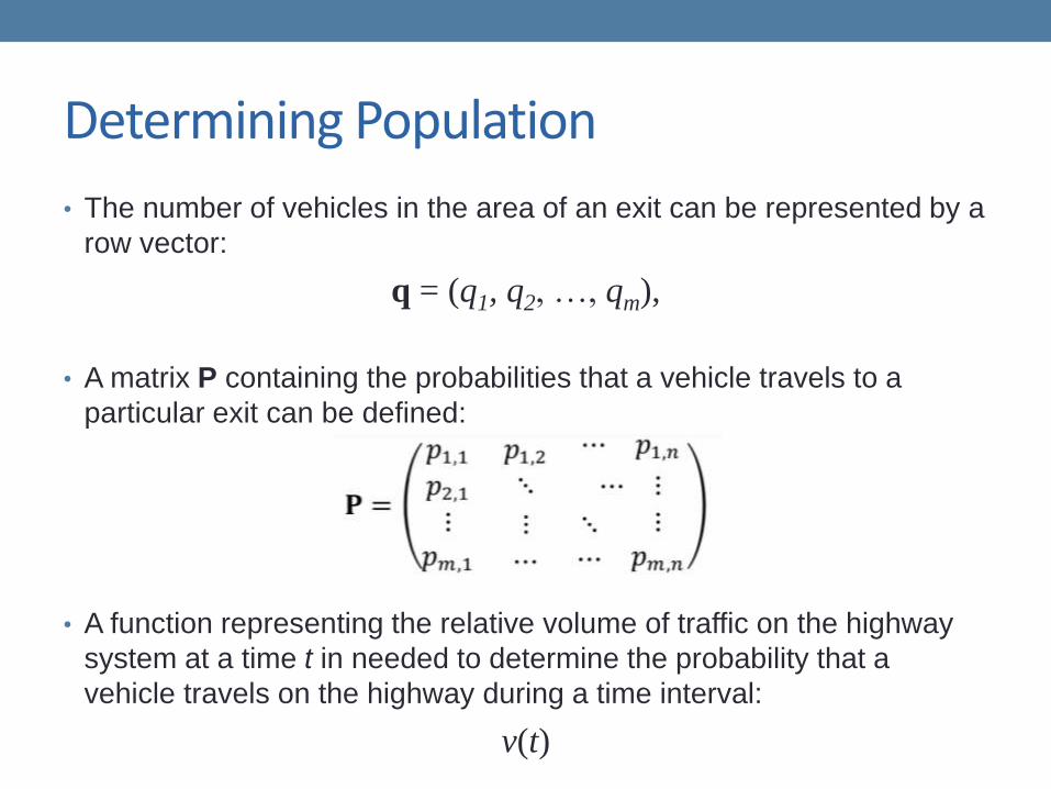
Determining Population
• The number of vehicles in the area of an exit can be represented by a
row vector:
q = (q1, q2, …, qm),
• A matrix P containing the probabilities that a vehicle travels to a
particular exit can be defined:
• A function representing the relative volume of traffic on the highway
system at a time t in needed to determine the probability that a
vehicle travels on the highway during a time interval:
v(t)
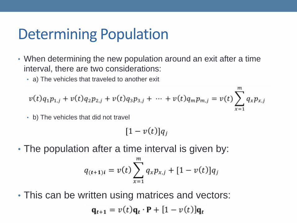
Determining Population
• When determining the new population around an exit after a time
interval, there are two considerations:
• a) The vehicles that traveled to another exit
• b) The vehicles that did not travel
• The population after a time interval is given by:
• This can be written using matrices and vectors:

Traffic Density
• In order to calculate the density of traffic on a segment of highway, we
must determine how many vehicles are traveling between exits during
a time interval. A route matrix describing the number of vehicles
going from one exit to another is defined:
• A matrix Q can be made from the population vector:

Traffic Density
• The route matrix can be rewritten using matrices:
• The number of vehicles passing through a segment of highway is the
sum of the vehicles traveling on all the routes that pass through this
segment:
• One way to determine which routes pass through a segment is to use
Dijkstra’s algorithm, which finds the shortest path between exits.

Traffic Density
• The density is then determined using the element ci,j , the average
speed of traffic, and the corresponding element of the matrix L:
• This is the predicted density for the segment from i to j
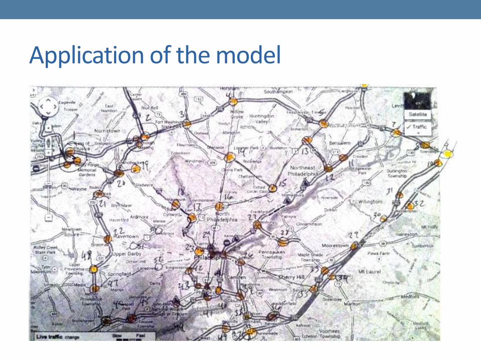
Application of the model
• Assumptions for this application:
• Only 46 exits are used in this model
• The initial number of vehicles at time 1AM is proportional to the number
of households in that area
• 3 transition matrices are used:
• From 5AM to 10AM – probability is proportional to the number of workers
• From 3PM to 4AM – probability is proportional to the number of households
• From 11AM to 2PM – the average of these two probabilities
• Average speed of vehicles is 65 mph
• False exits added to ends of highways that travel away from the network
in order to provide a buffer to the system
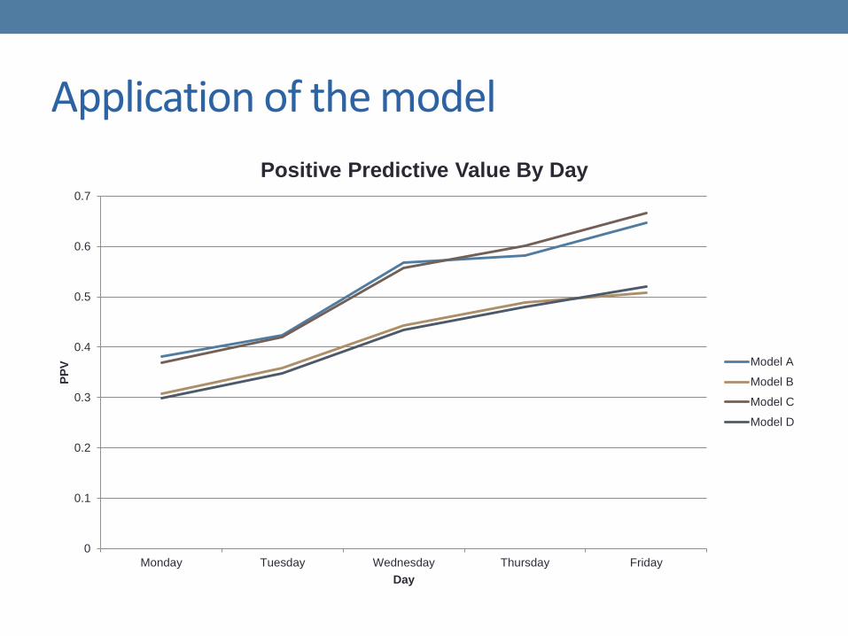
Application of the model
Application of the model
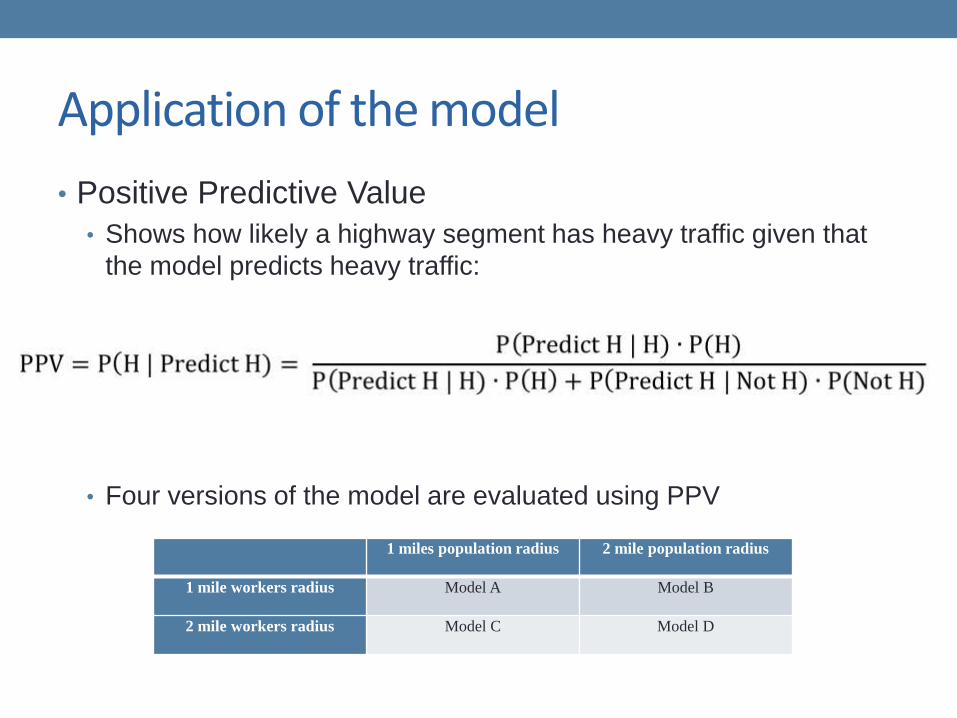
• Positive Predictive Value
• Shows how likely a highway segment has heavy traffic given that
the model predicts heavy traffic:
• Four versions of the model are evaluated using PPV
1 miles population radius 2 mile population radius
1 mile workers radius Model A Model B
2 mile workers radius Model C Model D

Application of the model
0
0.1
0.2
0.3
0.4
0.5
0.6
A B C D
PP
V
Model
Overall Positive Predictive Value
Application of the model
0
0.1
0.2
0.3
0.4
0.5
0.6
0.7
Monday Tuesday Wednesday Thursday Friday
PP
V
Day
Positive Predictive Value By Day
Model A
Model B
Model C
Model D

Application of the model
0
0.1
0.2
0.3
0.4
0.5
0.6
0.7
0.8
0.9
7 8 9 10 11 12 13 14 15 16 17 18 19
PP
V
Hour
Positive Predictive Value By Hour
Model A
Model B
Model C
Model D

References
Articles
Crisostomi, E., Kirkland, S., Schlote, A., & Shorten, R. (2010). A
Google-like Model of Road Network Dynamics and its Application to
Regulation and Control. International Journal of Control , 84 (3), 633-
651.
Dijkstra, E. W. (1959). A note on two problems in connexion with
graphs. Numerische mathematik , 1 (1), 269-271.
Dragoi, V.-A., & Dobre, C. (2011). A model for traffic control in urban
environments. Wireless Communications and Mobile Computing
Conference (IWCMC), 2011 7th International, (pp. 2139-2144).
Gazis, D. C., Herman, R., & Rothery, R. W. (1961). Nonlinear follow-
the-leader models of traffic flow. Operations Research , 9 (4), 545-567.
Hoogendoorn, S. P., & Bovy, P. H. (2001). State-of-the-art of vehicular
traffic flow modelling. Proceedings of the Institution of Mechanical
Engineers, Part I , 215 (4), 283-303.
Indrei, E. (2006). Markov Chains and Traffic Analysis. Department of
Mathematics, Georgia Institute of Technology .
Lighthill, M. J., & Whitham, G. B. (1955). On kinematic waves. II. A
theory of traffic flow on long crowded roads. Proceedings of the Royal
Society of London, Series A. Mathematical and Physical Sciences ,
229 (1178), 317-345.
Lim, S., Balakrishnan, H., Gifford, D., Madden, S., & Rus, D. (2011).
Stochastic Motion Planning and Applications to Traffic. International
Journal of Robotic Research .
Nagal, K., & Schreckenberg, M. (1992). A cellular automation model
for freeway traffic. Journal de Physique , 2 (12), 2221-2229.
Perrakis, K., Karlis, D., Cools, M., Janssens, D., & Wets, G. (2012). A
Bayesian approach for modeling origin-destination matrices.
Transportation Research Part A: Policy and Practice , 46 (1), 200-212.
Prigogine, I., & Andrews, F. C. (1960). A Boltzmann-like approach for
traffic flow. Operations Research , 8 (6), 789-797.
Rephann, T., & Isserman, A. (1994). New highways as economic
development tools: An evaluation using quasi-experimental matching
methods. Regional Science and Urban Economics , 24 (6), 723-751.
Sasaki, T., & Myojin, S. (1968). Theory of inflow control on an urban
expressway system. Proceedings of the Japan Society of Civil
Engineers , 160.
Transportation Reseach Board. (2011, March-April). Summary
minifeature on the HCM2010. Retrieved October 2013, from
Transportation Research Board:
onlinepubs.trb.org/onlinepubs/trnews/trnews273HCM2010.pdf

References
Van Zuylen, H. J., & Willumsen, L. G. (1980). The most likely trip matrix
estimated from traffic counts. Transportation Research Part B:
Methodological , 14 (3), 281-293.
Velasco, R., & Saayedra, P. (2008). Macroscopic Models in Traffic Flow.
Qualitative Theory of Dyanamical Systerms , 7 (1), 237-252.
Youngblom, E. (2013). Travel Time in Macroscopic Traffic Models for
Origin-Destination Estimation. University of Wisconsin-Milwaukee .
Zhang, G., Wang, Y., Wei, H., & Chen, Y. (2007). Examining headway
distribution models with urban freeway loop event data. Transportation
Research Record: Journal of the Transportation Research Board , 1999
(1), 141-149.
Data
Google Maps. (2013, October 20). Philadelphia, PA Historic Traffic Data
Map for Monday. Retrieved October 20, 2013, from Google Maps:
https://maps.google.com/maps
ITO Map. (2013, October 1). Highway Lanes. Retrieved October 1, 2013,
from ITO Map: http://www.itoworld.com/map/179
PennDOT. (2011). Factoring Process, Hourly Percent Total Vehicles.
Bureau of Planning and Research. PennDOT.
US Census Bureau. (2013, October 20). Demographic Snapshot
Summary, Total Households. Retrieved October 20, 2013, from Free
Demographics: http://www.freedemographics.com
US Census Bureau. (2013, Oct 20). Longitudinal-Employer Household
Dynamics Program. Retrieved Oct 20, 2013, from OnTheMap Application:
http://onthemap.ces.census.gov/
Images
Bailey, Simon F., and Rolf Bez. "Site specific probability distribution of
extreme traffic action effects." Probabilistic engineering mechanics 14.1
(1999): 19-26.
Masukura, Shuichi, Takashi Nagatani, and Katsunori Tanaka. "Jamming
transitions induced by a slow vehicle in traffic flow on a multi-lane
highway." Journal of Statistical Mechanics: Theory and Experiment
2009.04 (2009): P04002.
Treiber, M. and A. Kesting. “Phase Diagram of Traffic Patterns.” traffic-
states.com, http://www.traffic-states.com/?site=theorie&lang=en


