Application of an Algorithmically Differentiated

Turbomachinery Flow Solver to the Optimization of a

Fan Stage

Jan Backhaus∗, Andreas Schmitz∗, Christian Frey†

Institute of Propulsion Technology, German Aerospace Center (DLR)

Sebastian Mann‡, Marc Nagel§

MTU Aero Engines AG

Max Sagebaum¶, Nicolas R. Gauger‖

Chair for Scientific Computing, TU Kaiserslautern

The adjoint method has already proven its potential to reduce the computational effortfor optimizations of turbomachinery components based on flow simulations. However, thetransfer of the adjoint-based optimization methods to industrial design problems turns outto pose specific requirements to both the adjoint solver as well as the optimization algo-rithms which utilize the gradient information. While the construction of the adjoint solverthrough algorithmic differentiation is described in a parallel publication, we focus here onthe robust application of the gradient information in a high-dimensional multi-objective op-timization with several constraints including non-differentiated mechanical constraints. Wedescribe the optimization methods, which comprise the use of gradient-enhanced Krigingmeta-models, and subsequently apply these to the design optimization of a contra-rotatingfan stage. The results show that through the described combination of methods the adjointmethod can be used in practical design optimizations of turbomachinery components.

I. Introduction

The aerodynamic design of turbomachinery components relies to a large extent on computational fluiddynamics. Due to the steadily increasing environmental and economical demands and strict safety require-ments, design problems can become quite complex. Therefore, optimization techniques which help thedesigner to explore large design spaces, play an increasingly important role. Typically, optimizations areperformed using gradient-free techniques, e.g. evolutionary algorithms, since the deployed flow solvers do notprovide gradient information of their output quantities. However, the number of necessary design evaluationsincreases exponentially with the number of design variables, a phenomenon which is referred to as the curseof dimensionality.

The adjoint method can alleviate the limitation of the design space size by providing gradient informationat costs which are independent of the number of design variables. The large number of publications aboutadjoint flow solvers provides evidence of the interest in this method.1,2, 3, 4, 5, 6 Over the last two decadesadjoint-based optimization methods have been successfully used for simple airfoil designs. However, as thelimited number of publication shows, the transfer of the adjoint-based optimization methods to industrialdesign problems turns out to be less straightforward. To improve the applicability of the adjoint methodfor realistic designs, further efforts are required to improve both the adjoint solvers and the optimizationmethods.∗Phd. candidate, Institute of Propulsion Technology, German Aerospace Center (DLR), Cologne†Research Associate, Institute of Propulsion Technology, German Aerospace Center (DLR), Cologne‡Phd. candidate, MTU Aero Engines AG, Munich§Research Associate, MTU Aero Engines AG, Munich¶Phd. candidate, Chair for Scientific Computing, TU Kaiserslautern‖Professor, Chair for Scientific Computing, TU Kaiserslautern

1 of 20

American Institute of Aeronautics and Astronautics

This publication describes an approach for gradient-enhanced meta-model assisted optimization of tur-bomachinery, demonstrated on a contra-rotating fan stage with special focus on requirements from test-rigdesign practice. A parallel paper7 together with an earlier publication8 show how reverse mode differentiationplay together with elaborate performance optimizations to construct and maintain a consistent and efficientadjoint solver from a simulation code under frequent development. This paper mainly focuses on the efficientutilization of the gradient information. Here, we propose the use of gradient-enhanced meta-modeling anddiscuss the specific adaptation of this technique.

The paper is organized as follows: In section II we describe the specifics of the optimizations that in-fluenced our choice of methods, followed by a general description of optimizations using gradient-enhancedmeta-modeling and the specific implementation considerations. Subsequently we outline the choice of meth-ods for the flow simulation and summarize the development techniques for the discrete adjoint. This isfollowed by the application of these methods to the design optimization of a contra-rotating fan stage insection III.

II. Method

A. Choice of Methods

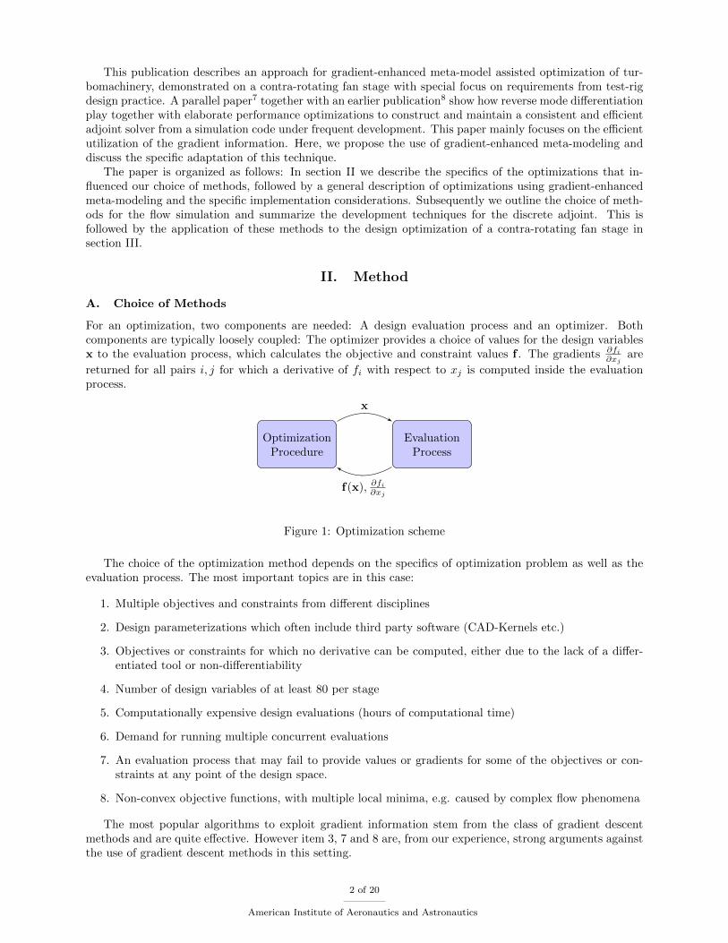
For an optimization, two components are needed: A design evaluation process and an optimizer. Bothcomponents are typically loosely coupled: The optimizer provides a choice of values for the design variablesx to the evaluation process, which calculates the objective and constraint values f . The gradients ∂fi

∂xjare

returned for all pairs i, j for which a derivative of fi with respect to xj is computed inside the evaluationprocess.

OptimizationProcedure

EvaluationProcess

x

f(x), ∂fi∂xj

Figure 1: Optimization scheme

The choice of the optimization method depends on the specifics of optimization problem as well as theevaluation process. The most important topics are in this case:

1. Multiple objectives and constraints from different disciplines

2. Design parameterizations which often include third party software (CAD-Kernels etc.)

3. Objectives or constraints for which no derivative can be computed, either due to the lack of a differ-entiated tool or non-differentiability

4. Number of design variables of at least 80 per stage

5. Computationally expensive design evaluations (hours of computational time)

6. Demand for running multiple concurrent evaluations

7. An evaluation process that may fail to provide values or gradients for some of the objectives or con-straints at any point of the design space.

8. Non-convex objective functions, with multiple local minima, e.g. caused by complex flow phenomena

The most popular algorithms to exploit gradient information stem from the class of gradient descentmethods and are quite effective. However item 3, 7 and 8 are, from our experience, strong arguments againstthe use of gradient descent methods in this setting.

2 of 20

American Institute of Aeronautics and Astronautics

gradient-enhanced Kriging (GEK) allows building a meta-model even when incomplete information ispresent at sampling points and provides a very flexible model which can adapt to a large range of functions.This flexibility comes for the price of computational effort to build a GEK model. Therefore we applyacceleration techniques to the training procedure as described in a following section.

B. Gradient assisted meta-modeling

Meta-ModelsOptimization

ProcedureEvaluation

Process

x

f(x), ∂fi∂xjf(x∗), s2(x∗)

Xs,Ys,∂Ys

∂Xs,x∗

Figure 2: Optimization with a gradient-enhanced meta-model

The basic information flow of gradient-enhanced meta-modeling is depicted in Fig. 2. The optimizationprocedure triggers the evaluation process for one choice of design variables x and obtains function and gra-dient values in return. However, the choice of where to evaluate the model is now determined by predictionsfrom the meta-models. These models are built from already sampled values Ys at the locations Xs, and thecorresponding gradient information ∂Ys

∂Xswhere available. Once built, the meta-models can inexpensively be

queried for function predictions f at unsampled points x∗. Additionally, the meta-models considered herealso return an estimated standard deviation of their prediction. This measure is useful for balancing theexploration of regions with missing samples and the exploitation of expected local minima. By optimizing onthe meta-model, the optimization procedure obtains a new point which can then be fed into the evaluationprocess.

The following section will describe how gradient-enhanced Kriging models are constructed and evaluatedin this work. For a more thorough description of the DGEK, the reader is referred to the cited publica-tions.9,10,11

C. Gradient-enhanced Kriging

In this section, we will first describe the gradient-free Kriging approach and then describe the extension todirect gradient-enhanced Kriging. The Kriging method models an unknown function f(x) as the realizationof a random variable Y by fitting a correlation structure of this variable to given observations. The model isconstructed based on a set of observations at sample points (xi, f(xi)), i ∈ {1, ..., D}, where xi ∈ RN . Thevector of observations Ys is defined as YT

s = [f(x1), ..., f(xD)] = [y1, ..., yD].Kriging predictions assume a spatial correlation between the observed samples in order to interpolate the

sampled values. This assumption is expressed through the choice of a correlation function which only dependson the weighted distance between two points. Gaussian or cubic spline functions are the most commonlyused forms of the spatial correlation function. In this work we use the Gaussian correlation function whichis defined as

Corr(xi,xj) =

N∏k=1

Corrk(θk,xi,xj) = exp

(−

N∑k=1

θk(xi,k − xj,k)2

). (1)

The parameters of the correlation function θk, k ∈ {1, ..., N}, the hyper-parameters, are used to adjustthe model to the observed data. This procedure is called training and is described later. If we assumethe parameters are already determined, the Kriging model can be evaluated as follows. The correlationsbetween all samples are arranged in a covariance matrix Covi,j = σ2Corr(xi,xj) ∈ RD×D, where σ denotesthe standard deviation of the Kriging process. With this matrix the ordinary Kriging predictor y and the

3 of 20

American Institute of Aeronautics and Astronautics

variance of the prediction of any point x in the design space can be obtained by

y(x) = β + cT (x)Cov−1(Ys − F), (2)

s2(x) =

(σ2 − cT (x)Cov−1c(x) +

(cT (x)Cov−1F− β)2

FTCov−1F

), (3)

with

ci(x) = Cov(x,xi),

FT = [β, ..., β] ∈ RD,

β =GTCov−1Ys

GTCov−1G,

GT = [1, ..., 1] ∈ RD.

Gradients can already be incorporated in these models, without any change to the formulation, by trans-forming gradients into artificial new samples and including these in the covariance matrix. This approach iscalled indirect gradient-enhanced Kriging. We follow a different approach, where the gradient information isdirectly included in the correlation matrix by introducing new correlation functions. These correlate func-tion values with gradients and gradients with gradients for any pair of sampling locations. These additionalcorrelations are obtained by differentiating the covariance function. The extended covariance matrix thenreads

Cov =

Cov(xi, xj)∂Cov(xi,xl)

∂xnl

︸ ︷︷ ︸D entries

∂Cov(xl,xi)

∂xnl ︸ ︷︷ ︸P entries

∂2Cov(xj ,xl)

∂xml ∂xnl

}

D entries}P entries

(4)

where k, l ∈ {1, ..., D} and n,m ∈ {1, ..., N} and P denotes the total number of observed derivatives. Ifpartial derivatives for each design parameter at all samples are provided then P = D · N and the matrixhas the dimension of D(1 + N) ×D(1 + N). This extended correlation matrix can be used in place of thepoint-point correlation matrix defined above. Therefore, we do not distinguish between both matrices. Withthis extended correlation matrix the extended vectors

YsT = [y1, ..., yD,

∂y1∂x1

, ...,∂yD∂xn

],

GT = [ 1, ..., 1︸ ︷︷ ︸D entries

, 0, ...0︸ ︷︷ ︸P entries

],

FT = [β, ..., β︸ ︷︷ ︸D entries

, 0, ...0︸ ︷︷ ︸P entries

],

ci(x)T = [Cov(x1,x), ...,Cov(xD,x),

∂Cov(x1,x)

∂x11, ...,

∂Cov(xD,x)

∂xnD],

the GEK predictor y and the GEK uncertainty s of the prediction for any point can still be calculated byequation (2) and (3). This direct gradient-enhanced Kriging (DGEK) approach is superior to the indirectapproach in terms of stability and accuracy of the model.12

D. Training

For the training of the hyper-parameters θk, the reduced maximum-likelihood approach is used, which aimsat finding the most likely model which produces the observed samples values and derivatives. This is achievedby minimizing the negative log-likelihood function with respect to the hyper-parameters θk:

` = − ln (det (Cov))− (Ys − F)TCov−1(Ys − F). (5)

4 of 20

American Institute of Aeronautics and Astronautics

Usually the variation of the data, σ, is computed analytically. However, as this is subject to a large samplingerror, we include σ as a hyper-parameter in the likelihood minimization iteration, which has proven to leadto better approximations.

To minimize the reduced likelihood, we employ the gradient descent method from the resilient backpropagation algorithm,13 which is a common algorithm in the training of artificial neural networks. Thenecessary partial derivatives of (5) with respect to θk are calculated as

∂`

∂θk= −Tr

(Cov−1 ∂Cov

∂θk

)+ (Ys − F)TCov−1 ∂Cov

∂θkCov−1(Ys − F)

To avoid the constraint θk > 0 in the maximum likelihood optimization and obtain a better scaling of

values, we define θk := eθk and use unconstrained minimization to find an optimal θk.

E. Optimization on the Meta-Model

The next point to be evaluated is obtained by optimizing on the meta-model. Obtaining predictions froma trained meta-model is comparatively cheap. While efficiency is not the main concern for the choice ofoptimization method, other aspects like simplicity and robustness are more important. Stochastic methodshave the advantage of producing different predictions, when repeatedly run on the same model, which isadvantageous when the evaluation chain fails to deliver function values for a prediction and therefore nomodel update takes place. Therefore we chose to use evolutionary algorithms to optimize on the meta-model. This optimization has to fulfill two requirements:

• Search regions of optimality for the best solution (exploitation)

• Reduce uncertainty about unsampled regions since they might also contain regions of optimality (ex-ploration)

It can be shown that an optimization, based only on the predicted values y would mainly focus on exploitationand might converge to non-optimal solutions (cf. section 3.2.1 in Forrester et al.14). This has to be consideredby formulating a dedicated objective function for the optimization on the meta-model. For single-objectiveoptimizations Jones et al.15 suggest the expected improvement criterion: The objective is to maximize theexpected value of the improvement over the currently best value.

In the case of multi-objective optimizations, this criterion must be extended, since there is no single bestsolution but a set of equally optimal solutions called Pareto front. A member, represented by its objectivevalues a = (a(1), ..., a(M)) dominates another member b = (b(1), ..., b(M)) if a(i) ≥ b(i) for all i = 1, 2, ...,M ,and a(i) > b(i) for some i. Furthermore, members that violate at least one constraint are dominated bymembers that fulfill all constraints. A solution which is not dominated by any other solution is calledPareto-optimal and the set of Pareto-optimal solutions is called Pareto front.

The gain from a new sample can be calculated as the volume gain by calculating the volume which isenclosed between the Pareto front Y and the new sample x:∏

i

(x(i) −max{y(i), y ∈ Y |y(i) < x(i)}

). (6)

If no sample in the Pareto front satisfies this criterion, the difference to a lower limit for the objectiveis used instead. In order to turn this criterion into a statistical prediction, the expected volume gain, weuse mean and variance from a location point in the meta-model to describe a multi-dimensional normaldistribution. By Monte-Carlo-Sampling of this distribution we obtain samples around the selected locationto calculate statistics of the above formulaa.

This objective can be minimized in two ways: Either by a prediction y with a lower mean than, or onewhere the expected value is worse than the current optimum, but with a high predicted variance s2. In thesecond case the high variance means, that the real observation can deviate from the predicted mean andthere is a chance that it could undercut the current optimum. The first mechanism will prefer exploitation.The second accounts for exploration of the model, since it will prefer samples in regions with high variance,which is caused by uncertainty over the real values at this point. Imposing a constraint on the variationof a prediction during the optimization on the meta-model allows shifting the balance from exploration toexploitation.

aIn order to predict multiple new members from one meta-model, the joint distribution of N models is built

5 of 20

American Institute of Aeronautics and Astronautics

F. Kriging regularization

A main difficulty, especially in gradient-enhanced Kriging, is that the covariance matrix easily becomesill-conditioned. The condition number can even reach magnitudes where the Cholesky algorithm fails toprovide a factorization of the matrix. In gradient.free Kriging this is often caused by highly correlatedsamples, e.g. sampling points becoming too close. Therefore a strategy that avoids placing sampling pointsclose to already known points would be optimal. However this cannot be assured during the optimization,since sampling points will naturally become clustered in regions of optimality. A well-known solution to thisproblem is to introduce a Tikhonov regularization - usually by adding a small constant to the main diagonalof the covariance matrix. In gradient-free Kriging an addition to the main diagonal corresponds to theassumption of random noise in the sampled values. This regularization eliminates the interpolation propertyof the Kriging method: already known points are no longer reproduced, but only approximated. Throughlarger regularization the model increasingly becomes a regression model. A very small regularization is oftenbeneficial, as simulation results are prone to a small random error since convergence to machine accuracy isnever achieved in practice.

It can be observed that gradient-enhanced Kriging tends to produce much larger condition numbers thangradient-free Kriging. The usual regularization with a constant addition to the main diagonal could beapplied to gradient-enhanced Kriging but would impair the prediction quality of the function values. Forthis reason and, since it is the additional gradient information that causes the ill-conditioning, we employ aslightly modified regularization

Cov + Γ

whereΓ = diag(δ δ · · · δ︸ ︷︷ ︸

D times

γ γ · · · γ︸ ︷︷ ︸P times

).

Two constants are used in this regularization scheme: δ > 0 is the regularization constant for the point-

point correlations and γ > 0 for the gradient-gradient part of the matrix. Since both Cov and Γ are positive

definite matrices this corresponds to a regularization of Cov. Note that the representation accuracy ofvalue information can be adjusted independently (e.g. using experience from gradient-free Kriging) from thegradient representation accuracy. This is a desirable property since we do not use predictions of gradientsbut only use the gradients to improve the prediction of values between samples.

Other authors propose the selective removal of correlations from the matrix which contribute the leastadditional information (e.g. pivoted Cholesky decomposition is used by Dalbey16) to improve the Krigingcondition number. Since the Kriging meta-model does not require full information on each sampling point,we also propose not to calculate the complete gradient information at all sampling points. In the applicationsection we demonstrate a simple criterion based on the number of evaluated points.

G. Flow simulations

Aerodynamic objectives are evaluated using DLR’s turbomachinery flow solver TRACE (for an overviewcf.17,18). The methods used in this work are exemplary for optimization simulations performed with thissolver. We calculate the steady state solution to the compressible Reynolds-averaged Navier-Stokes equationsin a rotating frame of reference using the ideal gas assumption. Turbulence is modelled by the Wilcox k-ω two equation turbulence model19 with modifications to correct the stagnation point anomaly20 and toaccount for rotational effects.21 The spatial discretization is based on a hybrid structured/unstructuredfinite volume approach; although completely structured grids have been used in this work. Convective fluxesare discretized using the MUSCL upwind approach with second-order accuracy and Harten’s entropy fix.A van Albada-type limiter is used to prevent oscillations in the vicinity of shocks (for the effect of fluxlimiters on differentiability cf.22). The wall boundary layer is modelled using wall functions. The solutionis obtained by implicit pseudo-time marching. Adjacent blade rows are coupled by Denton’s mixing plane23

approach. Non-reflecting boundary conditions24 are used to avoid unphysical reflections of waves at inlets,outlets and blade row interfaces. For a validation of the solver with experimental data for a contra-rotatingfan cf. Lengyel-Kampmann et al.25 .

6 of 20

American Institute of Aeronautics and Astronautics

H. Gradient Calculation

We calculate gradients of the aerodynamic objective functions through the discrete adjoint approach.26

For the implementation of the discrete adjoint solver to the existing CFD code we use the reverse mode ofalgorithmic differentiation (AD).27 However, an adjoint solver which is built by simply applying reverse-modeAD to the complete primal code leads to infeasibly high resource demands. For this reason, algorithmicdifferentiation is frequently combined with the more efficient manual differentiation. Many authors usemanual differentiation on the top level, e.g. for the time marching scheme and the spatial stencil, and usealgorithmic differentiation underneath for flux routines etc.28,29,3 A recent study describes how this techniquecan be applied to adjoin the flow solver under consideration.30 The third author originally developed anapproximate discrete adjoint through a combination of manual differentiation and finite differencing.31

However, experience shows that an approach which is driven by manual implementation becomes difficultto maintain. The continuing development on the primal code requires constant effort for updating or addingadjoint models. Since manual adjoining of involved CFD modules is a sophisticated task, there is at leasta lag between the availability of a primal simulation model and its adjoint - or primal models which arecompletely omitted. In case primal models with an existing adjoint are modified, the development lag canlead to inconsistent implementations and therefore wrong derivatives.32

Consequently we decided to use algorithmic differentiation to differentiate the whole code in a black boxfashion, which yields a complete and consistent, yet inefficient, adjoint solver and subsequently apply manualperformance optimizations through annotations in the primal code8.7 To describe these optimizations weregard the primal flow solver (including post processing) as a function of the mesh coordinates x ∈ Rn whichdelivers the vector of desired objective functions I ∈ Rm:

I = f(x).

Applying reverse mode differentiation to such a function allows to compute products of the function’s Jacobimatrix with a constant vector,

I∂f

∂x.

Here, the adjoint seed I ∈ Rm is usually chosen to be one output quantity

Ij =∂I

∂Ij= ej

with ej being the j-th unit vector. This is achieved by regarding the program as a chained sequence ofprimitive mathematical operations ϕi ∈ {+,−, ∗, /, sin, cos, exp, ...}, i = 1, .., l. We first calculate theresults of all primal operations

vi = ϕi(vj)j≺i.

Where (vj)j≺i is the list of variables on which the i-th operation depends. Afterwards we propagate thederivatives backward through the calculations in a reverse sweep:

vj =∑i≺j

vi∂

∂vjϕi(vj)j≺i j = l, ..., 1 .

The summation runs over all i which depend on the result of the j-th operation.From this relation, it can be seen that vj must be calculated in reverse order. However, we need the

values of the primal variables (vj)j≺i which can only be calculated in forward order. This is typically resolvedby storing all operations and intermediate results in the primal sweep in a sequential data structure calledtape. Nevertheless, this approach requires enough storage to accomodate this tape. Even though memorycan be traded in for run-time through checkpointing,33 the performance requirements are regarded too largefor practical simulations. Therefore performance improvements are necessary. We will briefly repeat the keypoints here, the techniques are described in detail in the parallel paper.7

Finding the steady state solution to the RANS equations is expressed by a flow state with a vanishingresidual:

R(u) = 0

The implicit pseudo time marching scheme used here can be written as

un+1 = un + P (un) ·∆u. (7)

7 of 20

American Institute of Aeronautics and Astronautics

Where P is an approximation to the Jacobian matrix of the residual ∂R∂u

∣∣un and the state update ∆u is

determined by solving the implicit system of equations(∆t−1 + P (un)

)∆u = Rn. (8)

We can regard this as an iterative procedure which produces a new flow state with each iteration

un+1 = G(x, un),

where G comprises the calculation of the residual and advancing the flow state. Note that the extraction ofthe iteration G and the identification of u as well as accounting for indirect dependence of G on x inside areal solver may be quite involved.

Simply differentiating the whole iteration loop over G by reverse mode AD would require recording alloperations and intermediate results which is infeasibly expensive. Assuming the iteration G converges to anattractive fixed point

u∗ = G(x, u∗)

whereR(u∗) = 0,

it is sufficient to only record one G iteration on this fixed point and generate an adjoint iteration by repeatedlypropagating the adjoint state u through this tape. A theorem of Christianson34 states, given that the primaliteration has converged to machine accuracy, the adjoint iteration procedure approaches the same convergencerate as the primal iteration.

About half of the tape size and computational time of the adjoint recurrence can be attributed to thesolution of the implicit system of equations. The implicit matrix

(∆t−1 + P (un)

)acts as a preconditioner

to the primal iteration procedure, which means that the flow solution will not depend on it - only theconvergence rate. Provided un is sufficiently close to fixed point, P (un) does not have to be recomputed forthe primal solver to converge. Consequently the dependencies of the preconditioner can be ignored duringthe recording of G. For the present solver, this reduces the memory consumption and run-time of the adjointsolver by a factor of two while leaving the convergence rate and results practically unaffected.

While both methods are quite effective in reducing the tape size, their prerequisite of R(u∗) = 0 is atheoretical one. Convergence to machine accuracy is never reached due to the stopping criteria of the solverand rounding errors. Some more complex simulations even stall at a larger residual due to the occurrence ofperiodic flow phenomena which cause the flow state only to converge to a limit cycle oscillation. Even whenthose primal solutions cannot be called converged, it can be observed that the integral quantities of interestconverge sufficiently accurate for practical purposes. While for a lot of these cases the adjoint recurrence stillconverges, there is no guarantee that it will do so. Stabilization of adjoints for oscillating primal solutions isan actively researched topic.35,36

The third measure for reducing the tape size is based on the observation that for some functions it ischeaper to store the complete Jacobian matrix than to store the computational tape. Obviously this is truefor functions with few input and output arguments but which comprise many internal operations. Thesefunctions are manually identified, must be free of side effects regarding the state vector and their input andoutput arguments have to be annotated. Then we can automatically calculate and store their Jacobi matrixwhile recording of the primal iteration, instead of their usual tape representation.

The code of the flow solver under consideration is developed in the C programming language, however aftersome modifications8 the code now also complies to the C++11 standard, which is sustained by automatictesting. This allows us to use reverse mode differentiation through operator overloading (OO) by usingdco/c++.37 For validation purposes we also use the reverse sweep of the full convergence trajectory withcheckpointing as well as the tangent forward mode.

III. Application

The application example is taken from a design optimization38 for a contra-rotating turbofan stage calledCRISP 2, which has recently been conducted at DLR. Starting from a test-rig designed and tested in the1990s, an extensive multidisciplinary optimization has been carried out to explore the potential of contra-rotating fan stages under the use of modern design, flow analysis and manufacturing techniques, especially

8 of 20

American Institute of Aeronautics and Astronautics

the use of CFRP-compound materials.39,40 CRISP 2 is a shrouded fan stage test-rig with two contra-rotatingrows, equipped with 10 and 12 blades with 1 meter in diameter at inflow. The final design has been builtand is about to be experimentally tested at DLR in the near future.

The original study was conducted using gradient-free meta-modelling in a chain of successive optimiza-tions. In order to use this as a benchmark case for this publication, we take one of the intermediate resultsfrom the later design cycles and optimize it using typical design objectives for a counter rotating fan.

ADP

NSP

mass flow rate [kg/s]

tota

l p

ressu

re r

atio

[­]

152 154 156 158 160 162

1.25

1.3

1.35

1.4

baseline geometry

Figure 3: Working line of the baseline member. (Blue areas depict aerodynamic constraints)

Role Name Symbol objective/constraint

1. Objective isentropic efficiency at ADP ηis,ADP increase/ [0.75,∞[

2. Objective total pressure ratio at NSP πtot,NSP increase/ [1.34,∞[

1. Constraint mass flow rate at ADP mADP [159.25, 159.75] kg/s

2. Constraint total pressure ratio at ADP πtot,ADP [1.28, 1.29]

3. Constraint mass flow rate at NSP mNSP [156, 157] kg/s

4. Constraint maximum Von Mises stress rotor 1 σv,R1 [−∞, 400] MPa

5. Constraint maximum Von Mises stress rotor 2 σv,R2 [−∞, 400] MPa

Table 1: Objectives and constraints

The baseline design is designed for a freestream velocity around Mach 0.68 with transonic flow (aroundMach 1.2) in the relative frame of reference. The stage produces a mass flow rate of 159 kg/s at a totalpressure ratio around 1.29. The main objective will be to improve the fan stage’s isentropic efficiency ηisat the aerodynamic design point (ADP). The ADP is fixed during the optimization by restricting the massflow rate to a range of 0.5 kg/s and the total pressure ratio to a range of 0.01 around the baseline. A typicaltrade off in turbomachinery design is that efficiency gains in the ADP reduce the stable operation range.Since the real operation range is hard to predict numerically, we use the stall margin criterion proposed byCumpsty which relates the operation range to the increase of total pressure ratio towards the surge line. Inorder to calculate this criterion we calculate a second operating point, the near stall point (NSP), which isdefined by a larger back pressure and has a 2.5% lower mass flow rate. A second objective function demandsthat the total pressure ratio in the NSP should be increased. The NSP is also restricted in its mass flow ratewith a tolerance margin of 1 kg/s and a lower bound to the total pressure ratio of 1.34. The operating pointsand their corresponding restrictions are depicted on the working line of the baseline geometry in Fig. 3.

9 of 20

American Institute of Aeronautics and Astronautics

A. Parameterization

The design is parameterized by a parametric CAD model based on 81 engineering parameters, influencingboth the blade and the flow path shape. A summary of the used parameters is given in Table 2.

number of parameters description

flow path

3 control point hub curve axial-shift

5 control point hub curve radial shift

5 control point casing curve radial shift

rotor 1 & 2

2 radial position of construction profile 2

6 stagger angles

12 angles at the leading edge

12 angles at the trailing edge

12 ellipse semi-axes at the leading edge

6 radii at the trailing edge

6 profile chord lengths

12 spline control point positions on the suction side

Table 2: Summary of the parameters

B. Mechanical modelling

Mechanical stability is a crucial restriction in design optimizations when the result is to be built and tested.Stability is usually assessed by mechanical calculations based on the FEM method, which are regularlyperformed using third party tools without a corresponding adjoint solver. Furthermore, some meaningfulmechanical constraints, like maximum stresses, are not continuously differentiable. In case the mechanicalconstraints can be evaluated sufficiently faster than the aerodynamic quantities, gradient-free mechanicalconstraints can still be regarded together with gradient-based aerodynamic objectives. Each constraint orobjective is modelled by its own meta-model and the position and number of observations from which themodel is built can differ. Therefore we create models for the mechanical constraints based on much moresamples than the aerodynamic objectives. In the described optimization we apply this technique by includingstatic calculations for the maximum von Mises stresses inside the blade. Even if an adjoint to the FEM toolwere available, this exact constraint would not be differentiable due to the maximum operator. From adesign of experiments containing 800 static FEM simulations we build a Kriging model, which is then usedby the optimizer to obtain predictions. The mechanical constraints are then evaluated for newly proposedmembers together with the aerodynamic objectives and are used to update the mechanical meta-model.

C. Practical training of the Kriging models

An efficient implementation of the gradient-enhanced Kriging model is essential, as the training procedurecan otherwise consume the computational saving from the adjoint gradients. The implementation inside theOptimization framework AutoOpti is described by Schmitz;41 the key points are summarized in the followingparagraphs.

The main issue is that the Kriging training incorporates operations on large dense matrices, whichhave a computational complexity of O(n3). The evaluation of the log-likelihood makes it necessary todetermine the inverse of the covariance matrix. The time spent on the inversion can be largely reduced bythe use of computational accelerators, more specifically general purpose graphics processing units (GPGPU).Furthermore highly tuned implementation of the log-likelihood and hand coded partial derivatives are usedfor the optimization.

In principle, the Kriging hyper-parameters have to be re-adjusted with every new infill from a designevaluation. However, often the information from an additional evaluation is in accordance with the currentchoice of model parameters, which can be easily determined by including the new point and evaluating thelikelihood with the current set of hyper-parameters. In this case the training procedure can be skipped,which considerably reduces the total costs for Kriging training throughout the optimization.

10 of 20

American Institute of Aeronautics and Astronautics

The largest training matrix obtained during the optimizations for this paper is approximately 4700×4700in size. When the meta-models have to be re-trained at this state, the total training time for all models (∼ 12minutes accelerated by an NVidia Quadro-K6000) is still an order of magnitude smaller than the functionand gradient evaluation (∼ 5 hours on an Intel Xeon E5-2650).

D. Design evaluation

The design evaluation is performed by a process chain in which all the values and gradients are calculated.This process chain consists, on a high level, of the following steps:

• Generation of solid surfaces

• Check for geometric constraints

• Generation of 3D meshes (FV and FEM)

• Finite element simulations

• RANS simulations

• RANS post-processing

First, the values of the design variables are inserted into a parametric CAD model to create splinesurface representations of all solid walls. Subsequently these surfaces are checked if they satisfy a setof geometric properties which are necessary for manufacturing and mechanical robustness. From thesesurfaces, 3D meshes are generated. This process up to this point is implemented in an in-house tool chain forturbomachinery design, belonging to the optimization suite AutoOpti. For the calculation of the mechanicalconstraints we use the FEM-Solver CalculiX.42 CFD Simulations are performed using the Navier-Stokessolver and corresponding postprocessor from DLR’s turbomachinery simulation suite TRACE.18,43 Afterthe simulations and their post-processing are finished, values for all objective functions and constraints areavailable.

Derivatives of CFD results are calculated by the adjoint method with the following process:

• Adjoint post-processing

• Adjoint RANS simulations

• Finite differences of surface and mesh generation

• Scalar product of perturbed meshes and adjoint solutions

The generation of solid surfaces and the meshes for simulation usually involves third party tools for whichno differentiated counterparts are available. Therefore, we apply small perturbations to one parameter at atime and re-run the whole process up to and including the mesh generation. This produces one perturbedmesh per parameter. These meshes can then be combined with each mesh sensitivity result from the adjointprocess by means of a dot product. This can be interpreted as the projection of the mesh sensitivity on amesh deformation obtained by finite differencing of the pre-process. This is based on the assumption, thatthe dependence of mesh nodes on the design parameters can be approximated by a linear relation in a certainrange and that the choice of step-width is much easier for the pre-process.

E. Gradient Validation

It is crucial for the optimization, that the adjoint gradients are consistent with the primal solver. Expe-rience shows that otherwise the optimization progress is slowed down up to a point where a gradient-freeoptimization advances faster. Inconsistent gradients also tend to worsen the ill-conditioning of the Krigingcorrelation matrix. To validate the gradient information, we employ calculations using the forward mode ofAD, as this mode is most simple to implement and therefore least error prone. Applying finite differenceswould be as simple; however the choice of step size is a very cumbersome task when fluid simulations areinvolved. Nevertheless, finite differences served as a tool for plausibility checks during the implementationof the full forward mode. Since the forward mode validation requires running 81 primal calculations, we

11 of 20

American Institute of Aeronautics and Astronautics

desgin parameter

se

ns

itiv

ity

va

lue

0 20 40 60 80

­0.001

­0.0005

0

0.0005

adjoint

forward ad1. objective

is,ADP

(a) Comparison of sensitvity values

desgin parameter

ab

s. e

rro

r

0 20 40 60 800

2E­07

4E­07

6E­07

8E­07

sensitivity error1. objective is,ADP

(b) Absolute error of the sensitivities

Figure 4: Validation of sensitivities for objective 1 at the baseline design by comparing forward AD andadjoint

chose to limit the validation to the ADP of the baseline geometry. Results can be seen in Fig. 4, wherethe results from the reverse mode differentiation including all performance optimizations are compared toa forward mode differentiation where no such optimizations are done and everything is consistently differ-entiated. Comparison of the gradient values (Fig. 4a) shows no visual difference, while in (Fig. 4b) it canbe seen that a difference exists, but it is smaller than 6 · 10−7. This difference is believed to be due to thestopping criteria of both the adjoint and forward mode differentiated solvers.

An impression how the convergence rate of the adjoint solver, which is itself linked to the primal solverresidual by Christianson’s theorem, relates to the evolution of the sensitivity value is given in Fig. 5.

adjoint iteration

res

idu

al L

1­n

orm

se

ns

itiv

ity

0 500 1000 1500 2000

10­6

10­5

10­4

10­3

10­2

1.4E­05

1.6E­05

1.8E­05

2E­05

2.2E­05

2.4E­05

2.6E­05

2.8E­05

parameter 5 sensitivity

adjoint residual

Figure 5: Convergence of the sensitivity value of parameter 5 in relation to the adjoint residual L1-norm

12 of 20

American Institute of Aeronautics and Astronautics

F. Optimizations

The main purpose of the application part of this paper is to demonstrate that adjoint simulations can beemployed for optimizations in a realistic setting. The second aim is to demonstrate, that the gradientinformation significantly improves the prediction quality of the meta-models and therefore improves theoptimization.

In order to demonstrate this, three optimizations have been performed:

1. without gradient information

2. with adjoint calculations for all sample points (fully gradient-enhanced)

3. with adjoint calculations for one in ten sample points (partly gradient-enhanced)

While the first and second optimization serves to show the influence of gradient information on theprediction, the third optimization is included to demonstrate the potential of sampling strategies that decidewhere to calculate gradient information.

All optimizations start by calculating the baseline design, which fulfills all constraints. Afterwards 3samples around the baseline member are created by randomly varying parameters of the baseline design.Each parameter is selected for variation with a probability of 20%. When selected, the parameter is modifiedby a normally distributed random offset with a standard deviation of 10% of the parameters variation range.Afterwards the optimization loop is started which comprises the following steps

1. Re-train meta-models based on the available samples if necessary.

2. Perform an optimization on the meta-models and try to find N members with the largest expectedvolume gain, with zero (or minimal) predicted distance to constraints.

3. Evaluate all objectives and constraints for the predicted members and calculate gradient informationif desired.

4. Include this information in a database of all evaluated samples.

Note that the steps are parallelized, which mean that at any time there are up to N evaluation processes,and steps 1 and 2 are run whenever one evaluation finishes.

iteration

res

idu

al l1

­no

rm

0 500 1000 150010

­6

10­5

10­4

10­3

10­2

10­1

primal calculation

reverse accumulation

ADP

(a) ADP

iteration

res

idu

al l1

­no

rm

0 500 1000 150010

­7

10­6

10­5

10­4

10­3

primal calculation

reverse accumulation

NSP

(b) NSP

Figure 6: Convergence of the adjoint solver for different operating points at the baseline design

Figure 6 shows the convergence of the adjoint solver for two operating points. The left part shows thesimulations for the ADP while the right part displays the convergence in the near stall point. The adjoint

13 of 20

American Institute of Aeronautics and Astronautics

simulation result

me

ta m

od

el p

red

icti

on

isentropic efficiency at ADP

y=x

error bars: 2pred

2 %

(a) First objective, gradient-free model

simulation resultm

eta

mo

de

l p

red

icti

on

isentropic efficiency at ADP

y=x

error bars: 2pred

2 %

(b) First objective, gradient-enhanced model

simulation result

me

ta m

od

el p

red

icti

on

­1.4 ­1.39 ­1.38 ­1.37 ­1.36 ­1.35 ­1.34 ­1.33

­1.4

­1.39

­1.38

­1.37

­1.36

­1.35

­1.34

­1.33

total pressure ratio at NSPy=x

error bars: 2pred

(c) Second objective, gradient-free model

simulation result

me

ta m

od

el p

red

icti

on

­1.4 ­1.38 ­1.36 ­1.34­1.4

­1.39

­1.38

­1.37

­1.36

­1.35

­1.34total pressure ratio at NSPy=x

error bars: 2pred

(d) Second objective, gradient-enhanced model

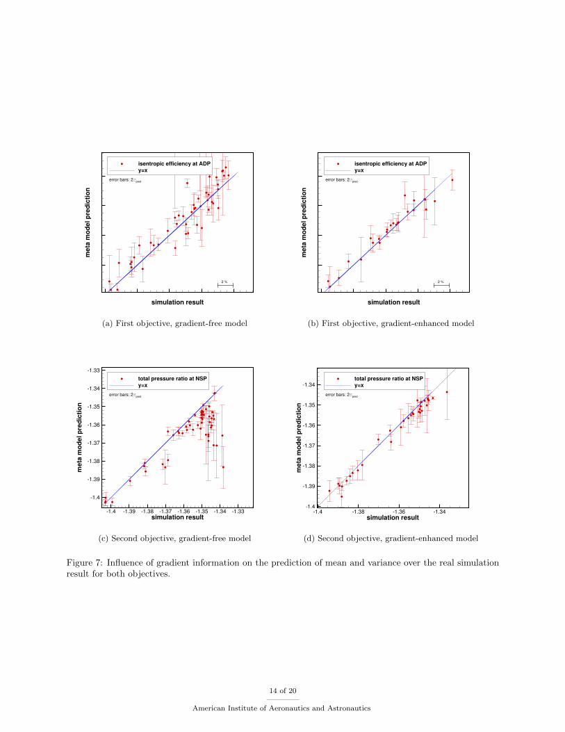
Figure 7: Influence of gradient information on the prediction of mean and variance over the real simulationresult for both objectives.

14 of 20

American Institute of Aeronautics and Astronautics

solver converges satisfactory in both operating points and exhibits the same residual reduction rate as theprimal solver.

The key assessment criterion for the prediction quality of a meta-model is the error between the statisticalprediction and the evaluation of the simulation model. Figure 7 displays the predictions produced by themeta-models for the objectives in the gradient-free and fully gradient-enhanced optimization. The predictionis displayed as the mean value together with the error bar denoting the confidence interval of the prediction2σ on the y axis. The observed simulation is represented on the x axis. With a perfect model both wouldbe identical and would therefore lie on the blue line. The closer a point is to the blue line, the better wasthe corresponding prediction. However, a good prediction of the variance is equally important, since thisinfluences the choice of sampling through the expected volume gain criterion. It can be seen that the gradient-free optimization (7a and 7c) has points with greater distance to the line of perfect prediction and also morepoints for which the true value does not lie within the confidence interval of 2σ. Both criteria are muchbetter met for the gradient based optimization (7b, 7d). Note that for the gradient-free optimization, onlyevery other point is plotted to maintain clarity. The evolution of the meta-models prediction error during

Optimization iteration

ab

s. p

red

icti

on

err

or

0 50 100 150

0

0.05

0.1

0.15gradient free

with gradients

1. objective: is,ADP

(a) 1. Objective Function

Optimization iteration

ab

s. p

red

icti

on

err

or

50 1000

0.005

0.01

0.015

0.02

0.025

0.03

0.035

0.04

0.045

0.05

0.055

0.06

gradient free

with gradients

2. objective: tot,NSP

(b) 2. Objective Function

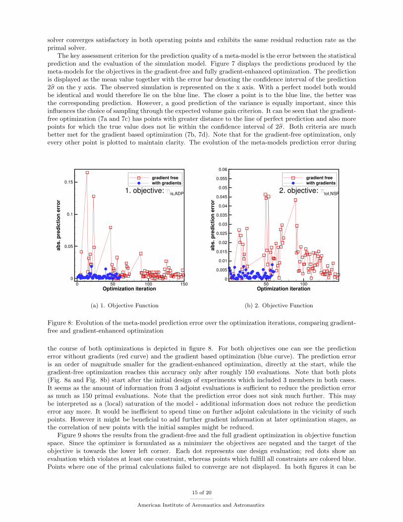
Figure 8: Evolution of the meta-model prediction error over the optimization iterations, comparing gradient-free and gradient-enhanced optimization

the course of both optimizations is depicted in figure 8. For both objectives one can see the predictionerror without gradients (red curve) and the gradient based optimization (blue curve). The prediction erroris an order of magnitude smaller for the gradient-enhanced optimization, directly at the start, while thegradient-free optimization reaches this accuracy only after roughly 150 evaluations. Note that both plots(Fig. 8a and Fig. 8b) start after the initial design of experiments which included 3 members in both cases.It seems as the amount of information from 3 adjoint evaluations is sufficient to reduce the prediction erroras much as 150 primal evaluations. Note that the prediction error does not sink much further. This maybe interpreted as a (local) saturation of the model - additional information does not reduce the predictionerror any more. It would be inefficient to spend time on further adjoint calculations in the vicinity of suchpoints. However it might be beneficial to add further gradient information at later optimization stages, asthe correlation of new points with the initial samples might be reduced.

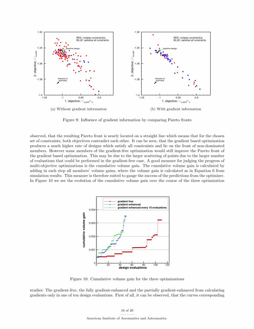
Figure 9 shows the results from the gradient-free and the full gradient optimization in objective functionspace. Since the optimizer is formulated as a minimizer the objectives are negated and the target of theobjective is towards the lower left corner. Each dot represents one design evaluation; red dots show anevaluation which violates at least one constraint, whereas points which fulfill all constraints are colored blue.Points where one of the primal calculations failed to converge are not displayed. In both figures it can be

15 of 20

American Institute of Aeronautics and Astronautics

baseline design

direction ofoptimality

1. objective: ­is,ADP

/0

2. o

bje

ctive

: ­

tot,

NS

P

­1.05 ­1 ­0.95 ­0.9­1.4

­1.38

­1.36

­1.34

­1.32

RED: violates constraint(s)BLUE: satisfies all constraints

(a) Without gradient information

baseline design

direction ofoptimality

1. objective: ­is,ADP

/0

2. o

bje

ctive

: ­

tot,

NS

P

­1.05 ­1 ­0.95 ­0.9­1.4

­1.38

­1.36

­1.34

­1.32

RED: violates constraint(s)BLUE: satisfies all constraints

(b) With gradient information

Figure 9: Influence of gradient information by comparing Pareto fronts

observed, that the resulting Pareto front is nearly located on a straight line which means that for the chosenset of constraints, both objectives contradict each other. It can be seen, that the gradient based optimizationproduces a much higher rate of designs which satisfy all constraints and lie on the front of non-dominatedmembers. However some members of the gradient-free optimization would still improve the Pareto front ofthe gradient based optimization. This may be due to the larger scattering of points due to the larger numberof evaluations that could be performed in the gradient-free case. A good measure for judging the progress ofmulti-objective optimizations is the cumulative volume gain. The cumulative volume gain is calculated byadding in each step all members’ volume gains, where the volume gain is calculated as in Equation 6 fromsimulation results. This measure is therefore suited to gauge the success of the predictions from the optimizer.In Figure 10 we see the evolution of the cumulative volume gain over the course of the three optimization

design evaluations

cu

mu

lati

ve

vo

lum

e g

ain

0 20 40 60 80 100 1200

0.001

0.002

0.003

0.004

gradient free

gradient enhanced

gradient enhanced every 10 evaluations

Figure 10: Cumulative volume gain for the three optimizations

studies: The gradient-free, the fully gradient-enhanced and the partially gradient-enhanced from calculatinggradients only in one of ten design evaluations. First of all, it can be observed, that the curves corresponding

16 of 20

American Institute of Aeronautics and Astronautics

to gradient-enhanced optimizations feature a much higher slope and therefore show that both gradient-enhanced optimizations lead to more improvement per evaluation than the gradient-free optimization. Onecan observe various plateaus in each curve which stem from evaluations that either violate a constraintor turned out not to lie on the Pareto front. Both phenomena are caused by the prediction error of themeta-models. Both gradient-enhanced optimizations are comparable in slope, from which we can conclude,that evaluating gradients only for every tenth member delivers sufficient information. Further research intogood decision criteria on where to calculate gradient information seems promising. It can be observed, thatthe partly gradient-enhanced optimization sometimes even advances faster than the fully gradient-enhancedoptimization - however this could very well be an artifact from the stochastic optimization on the meta-models. Owing to this stochastic nature of the optimization measurements of the time saving through theadjoint method must be repeatedly performed under controlled circumstances and will be therefore left toanother publication. However, it can be stated that in case of the fully gradient-enhanced optimization, allperformance gains are absorbed by the additional effort for the adjoint evaluations. However the partiallygradient-enhanced optimization offers a performance improvement over the gradient-free optimization.

Figure 11: Comparison of cross sections on both rotors of baseline and most efficient member from thegradient based optimization

The optimization result is depicted in Fig. 11 as a comparison of all construction profiles between thebaseline geometry and the most efficient member from the gradient-enhanced optimization.

An aerodynamic comparison of the working lines for both configurations is displayed in Fig. 12. Fromthe working line (Fig. 12a) it can be seen that the optimized geometry is at the upper limit of the massflow rate in the ADP and at the lower limits of mass flow rate and total pressure ratio in the NSP. This isanother indication, that efficiency gains in the ADP (can be seen in Fig. 12b) are partly reached through atthe expense of worsening the stall margin criterion. Note that the optimized geometry seems to feature alonger operating line. However this cannot be determined from the plots due to the large offset between thecalculated operating points at the stall margin.

17 of 20

American Institute of Aeronautics and Astronautics

ADP

NSP

mass flow rate [kg/s]

tota

l p

ressu

re r

atio

[­]

150 152 154 156 158 160 1621.2

1.25

1.3

1.35

1.4

baseline geometry

most efficient geometry

(a) total pressure ratio

ADPNSP

mass flow rate [kg/s]

ise

ntr

op

ic e

ffic

iency (

no

rmaliz

ed

) [­

]

150 152 154 156 158 160

0.9

0.95

1

1.05

1.1

baseline geometry

most efficient geometry

(b) isentropic efficiency

Figure 12: Comparison of the initial member and most efficient member as speed lines

IV. Conclusion

The main objective of this paper is to demonstrate that the adjoint method is suited to improve thedesign of turbomachinery components in a realistic scenario. We show how practical necessities influencethe choice of methods. To maintain the consistency to a constantly changing primal solver we use reversemode algorithmic differentiation with subsequent performance improvements. We base the optimization ongradient-enhanced meta-modelling in order to achieve robustness against failure in the evaluation chain.The processes are described, assuming that non-adjoined tools are involved. We show that the surface- andmesh-generation tools can be included by finite differencing and finite element calculations without adjointsusing a meta-modelling with finer sampling. The results show, that the gradients significantly improve thepredictions for objective function and for the constraints. This leads to a steeper increase of volume gain aswell as a higher rate of members that satisfy the constraints as well as a denser Pareto front. Results fromthe analysis of the evolution of the prediction indicate, that it is more efficient to calculate gradients onlyat selected sample points. Research into schemes for choosing where to calculate gradient information mayoffer significant improvement over the methods described here.

V. Acknowledgement

This project has received funding from the Clean Sky 2 Joint Undertaking under the European UnionsHorizon 2020 research and innovation programme under grant agreement No [CS2-Engines ITD-2014-2015-01].

References

1Newman III, J. C., Taylor III, A. C., Barnwell, R. W., Newman, P. A., and Hou, G. J.-W., “Overview of sensitivityanalysis and shape optimization for complex aerodynamic configurations,” Journal of Aircraft , Vol. 36, No. 1, 1999, pp. 87–96.

2Duta, M. C., Shahpar, S., and Giles, M. B., “Turbomachinery design optimization using automatic differentiated adjointcode,” ASME Turbo Expo 2007: Power for Land, Sea, and Air , American Society of Mechanical Engineers, 2007, pp. 1435–1444.

3Marta, A. C., Shankaran, S., Holmes, D. G., and Stein, A., “Development of Adjoint Solvers for Engineering Gradient-Based Turbomachinery Design Applications,” Proceedings of the ASME Turbo Expo 2009 , Vol. Volume 7: Turbomachinery,Parts A and B, June 2009.

4Peter, J. E. and Dwight, R. P., “Numerical sensitivity analysis for aerodynamic optimization: A survey of approaches,”Computers & Fluids, Vol. 39, No. 3, 2010, pp. 373–391.

5Wang, D. X., He, L., Li, Y. S., and Wells, R. G., “Adjoint Aerodynamic Design Optimization for Blades in MultistageTurbomachines—Part II: Validation and Application,” Journal of Turbomachinery, Vol. 132, No. 2, 2010, pp. 021012.

6Backhaus, J., Aulich, M., Frey, C., Lengyel, T., and Voß, C., “Gradient Enhanced Surrogate Models Based on AdjointCFD Methods for the Design of a Counter Rotating Turbofan,” Proceedings of the ASME Turbo Expo 2012 , 2012.

18 of 20

American Institute of Aeronautics and Astronautics

7Sagebaum, M., Ozkaya, E., Gauger, N. R., Backhaus, J., Frey, C., Mann, S., and Nagel, M., “Efficient AlgorithmicDifferentiation Techniques for Turbo-machinery Design,” submitted for publication, AIAA-Paper , Vol. ???, 2017, pp. ???

8Sagebaum, M., Ozkaya, E., and Gauger, N. R., “Challenges in the automatic differentiation of an industrial CFD solver,”Evolutionary and Deterministic Methods for Design, Optimization and Control with Application to Industrial and SocietalProblems (EUROGEN 2013), 2013.

9Sobester, A. and Forrester, A., Aerospace Series : Aircraft Aerodynamic Design : Geometry and Optimization, Wiley,2014.

10Yamazaki, W., Rumpfkeil, M. P., and Mavriplis, D. J., “Design optimization utilizing gradient/hessian enhanced surrogatemodel,” AIAA Paper , Vol. 4363, 2010, pp. 2010.

11Han, Z.-H., Gortz, S., and Zimmermann, R., “Improving adjoint-based aerodynamic optimization via gradient-enhancedKriging,” 50th AIAA Aerospace Sciences Meeting including the New Horizons Forum and Aerospace Exposition, Nashville,Tennessee, 2012.

12Zimmermann, R., “On the maximum likelihood training of gradient-enhanced spatial gaussian processes,” SIAM Journalon Scientific Computing, Vol. 35, No. 6, 2013, pp. A2554–A2574.

13Riedmiller, M. and Braun, H., “A direct adaptive method for faster backpropagation learning: The RPROP algorithm,”Neural Networks, 1993., IEEE International Conference On, IEEE, 1993, pp. 586–591.

14Forrester, A., Sobester, A., and Keane, A., Engineering Design via Surrogate Modelling: A Practical Guide, Wiley, 2008.15Jones, D. R., Schonlau, M., and Welch, W. J., “Efficient global optimization of expensive black-box functions,” Journal

of Global optimization, Vol. 13, No. 4, 1998, pp. 455–492.16Dalbey, K. R., “Efficient and Robust Gradient Enhanced Kriging Emulators,” SANDIA REPORT SAND2013-7022,

Sandia Natianal Laboratories, Sandia National Laboratories Albuquerque, New Mexico 87185 and Livermore, California 94550,August 2013.

17Yang, H., Nurnberger, D., and Kersken, H.-P., “Towards Excellence in Turbomachinery Computational Fluid Dynamics,”Journal of Turbomachinery, Vol. 2006, No. 128, 2006, pp. 390–402.

18Becker, K., Heitkamp, K., and Kugeler, E., “Recent Progress In A Hybrid-Grid CFD Solver For Turbomachinery Flows,”Proceedings Fifth European Conference on Computational Fluid Dynamics ECCOMAS CFD 2010 , 2010.

19Wilcox, D. C., “Reassessment of the Scale-Determining Equation for Advanced Turbulence Models,” AIAA Journal ,Vol. 26, No. 11, Nov. 1988, pp. 1299–1310.

20Kato, M. and Launder, B. E., “The Modeling of Turbulent Flow Around Stationary and Vibrating Square Cylinders,”9th Symposium on Turbulent Shear Flows, 1993, pp. 10.4.1–10.4.6.

21Bardina, J., Ferziger, J. H., and Rogallo, R. S., “Effect of rotation on isotropic turbulence: computation and modelling,”J. Fluid Mech., Vol. 154, 1985, pp. 321–336.

22Engels-Putzka, A., Backhaus, J., and Frey, C., “On the usage of finite differences for the development of discrete linearisedand adjoint CFD solvers,” Proceedings of the 6th. European Conference on Computational Fluid Dynamics - ECFD VI , editedby E. Onate, X. Oliver, and A. Huerta, Juli 2014.

23Denton, J. D., “The Calculation of Three-Dimensional Viscous Flow Through Multistage Turbomachines,” Journal ofTurbomachinery, Vol. 114, No. 1, Jan. 1992, pp. 18–26.

24Giles, M. B., “Nonreflecting Boundary Conditions for Euler Calculations,” AIAA Journal , Vol. 28, No. 12, 1990, pp. 2050–2058.

25Lengyel-Kampmann, T., Bischoff, A., Meyer, R., and Nicke, E., “Design of an economical counter rotating Fan: com-parison of the calculated and measured steady and unsteady results,” ASME Turbo Expo 2012: Turbine Technical Conferenceand Exposition, American Society of Mechanical Engineers, 2012, pp. 323–336.

26Giles, M. B. and Pierce, N. A., “An introduction to the adjoint approach to design,” Flow, turbulence and combustion,Vol. 65, No. 3-4, 2000, pp. 393–415.

27Griewank, A., Evaluating Derivatives: Principles and Techniques of Algorithmic Differentiation (Frontiers in AppliedMathematics), Society for Industrial and Applied Mathematics, 2000.

28Giles, M., Ghate, D., and Duta, M., “Using automatic differentiation for adjoint CFD code development,” 2005.29Mader, C. A., RA Martins, J., Alonso, J. J., and Der Weide, E. V., “ADjoint: An approach for the rapid development

of discrete adjoint solvers,” AIAA journal , Vol. 46, No. 4, 2008, pp. 863–873.30Backhaus, J., Engels-Putzka, A., and Frey, C., “a code-coupling approach to the implementation of discrete adjoint solvers

based on automatic differentiation,” VII European Congress on Computational Methods in Applied Sciences and Engineering,ECCOMAS Congress 2016 , June 2016.

31Frey, C., Kersken, H.-P., and Nurnberger, D., “The discrete adjoint of a turbomachinery RANS solver,” ASME TurboExpo 2009: Power for Land, Sea, and Air , American Society of Mechanical Engineers, 2009, pp. 345–354.

32Dwight, R. P. and Brezillon, J., “Effect of approximations of the discrete adjoint on gradient-based optimization,” AIAAjournal , Vol. 44, No. 12, 2006, pp. 3022–3031.

33Griewank, A. and Walther, A., “Algorithm 799: revolve: an implementation of checkpointing for the reverse or adjointmode of computational differentiation,” ACM Transactions on Mathematical Software (TOMS), Vol. 26, No. 1, 2000, pp. 19–45.

34Christianson, B., “Reverse accumulation and attractive fixed points,” Optimization Methods and Software, Vol. 3, No. 4,1994, pp. 311–326.

35Dwight, R. P. and Brezillon, J., “Efficient and robust algorithms for solution of the adjoint compressible Navier–Stokesequations with applications,” International journal for numerical methods in fluids, Vol. 60, No. 4, 2009, pp. 365–389.

36Albring, T., Dick, T., and Gauger, N. R., “Assessment of the Recursive Projection Method for the Stabilization ofDiscrete Adjoint Solvers,” submitted for publication, AIAA-Paper , Vol. ???, 2017, pp. ???

37Naumann, U., “DCO Short Introduction,” Tech. rep., NAG, 2015.38Lengyel-Kampmann, T., Vergleichende aerodynamische Untersuchungen von gegenlaufigen und konventionellen

Fanstufen fur Flugtriebwerke, Phd thesis, Ruhr-Universitat Bochum, August 2015.

19 of 20

American Institute of Aeronautics and Astronautics

39Gorke, D., Le Denmat, A.-L., Schmidt, T., Kocian, F., and Nicke, E., “Aerodynamic and mechanical optimization ofCF/PEEK blades of a counter rotating fan,” Proceedings of the ASME Turbo Expo 2012 , 2012.

40Aulich, A.-L., Goerke, D., Blocher, M., Nicke, E., and Kocian, F., “Multidisciplinary automated optimization strategyon a counter rotating fan,” ASME Turbo Expo 2013: Turbine Technical Conference and Exposition, American Society ofMechanical Engineers, 2013, pp. V06BT43A007–V06BT43A007.

41Schmitz, A., “Entwicklung eines objektorientierten und parallelisierten Gradient Enhanced Kriging Ersatzmodells,” Tech.rep., Fernuniversitat Hagen, September 2013, in German, http://elib.dlr.de/85734/.

42Dhondt, G., The finite element method for three-dimensional thermomechanical applications, John Wiley & Sons, 2004.43Voigt, C., Wellner, J., Morsbach, C., and Kugeler, E., “Conquer the Terabyte-scale: Post-processing of high resolution

unsteady CFD data for turbomachinery analysis,” 6th European Congress on Computational Methods in Applied Sciences andEngineering (ECCOMAS 2012), Vienna, Austria, Sept. 2012.

20 of 20

American Institute of Aeronautics and Astronautics