Application of Bayesian Inference Techniques for Calibrating Eutrophication Models

by

Weitao Zhang

A thesis submitted in conformity with the requirements

for the degree of Master of Science

Graduate Department of Geography

University of Toronto

© Copyright by Weitao Zhang (2008)

Application of Bayesian Inference Techniques for Calibrating Eutrophication Models

by Weitao Zhang (2008) for the degree of Master of Science,

Graduate Department of Geography, University of Toronto

Abstract This research aims to integrate mathematical water quality models with Bayesian

inference techniques for obtaining effective model calibration and rigorous assessment of

the uncertainty underlying model predictions. The first part of my work combines a

Bayesian calibration framework with a complex biogeochemical model to reproduce

oligo-, meso- and eutrophic lake conditions. The model accurately describes the observed

patterns and also provides realistic estimates of predictive uncertainty for water quality

variables. The Bayesian estimations are also used for appraising the exceedance

frequency and confidence of compliance of different water quality criteria. The second

part introduces a Bayesian hierarchical framework (BHF) for calibrating eutrophication

models at multiple systems (or sites of the same system). The models calibrated under the

BHF provided accurate system representations for all the scenarios examined. The BHF

allows overcoming problems of insufficient local data by “borrowing strength” from

well-studied sites. Both frameworks can facilitate environmental management decisions.

I

 

Acknowledgments Foremost, I would like to express my deepest gratitude to my advisor, Prof.

George Arhonditsis, for his encouragement, patience, support, and constant invaluable

advice. I have been amazingly fortunate to have him as an advisor, who has the rich

knowledge and perspicacious intuition on ecological modeling problems. I enjoyed my

research experience so much during last two years.

I would also like to give a special thanks to my committee, Prof. Myrna Simpson

and Prof. Miriam Diamond, for volunteering their time and providing me their feedback

through this process.

At the same time, I wish to thank all the members of the Ecological Modeling Lab

for their help. We also spent great times together just for random talks that usually had

nothing to do with modeling.

Finally, I would like to give thanks to my parents for all their love and support

throughout my life. I also would like to dedicate this to my wife, Jing Wu, for all her

support while I pursued my educational goals and for enduring all the evenings and

weekends that I was busy with school. I am finally done!

This work was supported by Ontario Graduate Scholarship (OGS) and funding

from the Department of Geography, University of Toronto.

II

 

Table of Contents Abstract……………………………………..…………………………………………I

Acknowledgments…………………………..…………..………………………………II

Table of Contents………………..………….…………………………………………III

List of Tables…………………………………………………………………………….V

List of Figures…………………….………………………….…………………………VI

List of Appendices………………….…………………..……….……………………VIII

Glossary of Terms………………….…………………………………..………………IX

Chapter 1 Introduction…………….…..……………………..…………………………1

Chapter 2 Predicting the Frequency of Water Quality Standard Violations

Using Bayesian Calibration of Eutrophication Models……..………..…5

2.1 Introduction………………..……………………………………………………5

2.2 Methods…...…….………………………………………………………………9

2.2.1 Model Description……………………..………………………………9

2.2.2 Bayesian Framework…………………….……………………………13

2.3 Results……….……….…………………………………………………………18

2.4 Discussion…….……….….……..………………………………………………23

2.5 Conclusions…….………………..………………………………………………28

Tables…….……..……..……...……..………………………………………………31

Figures…….…….…….….…….…...………………………………………………34

Chapter 3 A Bayesian Hierarchical Framework for Calibrating Aquatic 3 4

Biogeochemical Models ………..…………………………………………43

3.1 Introduction………………..……………………………………………………43

3.2 Methods…...…….………………………………………………………………47

3.2.1 Bayesian Hierarchical Framework…….………………….……………50

3.2.2 Mathematical model......………….……….……………………………53

III

 

3.2.3 Numerical approximations for posterior distributions……………….…55

3.2.4 Model updating……….………….……..………………………………56

3.3 Results…………………………..………………………………………………56

3.4 Discussions and Conclusions ….…….….……..…………….…………………61

Tables….……..…….….……..……..………………………………………………68

Figures….………….……..….……..………………………………………………72

Chapter 4 Future Research Perspectives…………….……..…………………………85

References…………………………………….……….……..…………………………89

Appendices……………………..…………….……….……..…………………………99

IV

 

List of Tables Table 2.1 Prior and posterior parameter distributions in three trophic states……………31

Table 2.2 Goodness-of-fit statistics for the model state variables......…….……..………32

Table 2.3 Posterior estimates of the mean values and standard deviations

of the model discrepancies..................................................................................33

Table 3.1 The scenarios examined under the Bayesian hierarchical configuration

of the mathematical model..................................................................................68

Table 3.2 The prior probability distributions of the hyperparameters................................69

Table 3.3 Scenario C. Posterior estimates of the mean values and standard

deviations of the model stochastic nodes............................................................70

Table 3.4 Scenario E. Posterior estimates of the mean values and standard

deviations of the model stochastic nodes............................................................71

V

 

List of Figures

Figure 2.1 The structure of the complex aquatic biogeochemical model.........................34

Figure 2.2 Prior and posterior cumulative distributions of the aquatic

biogeochemical model......................................................................................36

Figure 2.3 Comparison between the observed and posterior predictive monthly

distributions for 10 water quality variables in the oligotrophic environment...37

Figure 2.4 Comparison between the observed and posterior predictive monthly

distributions for 10 water quality variables in the mesotrophic environment...38

Figure 2.5 Comparison between the observed and posterior predictive monthly

distributions for 10 water quality variables in the eutrophic environment.......39

Figure 2.6 Predictive distributions for water quality variables of management

interest during the summer stratified period (June to September)...................40

Figure 2.7 The exceedance frequency and confidence of compliance of the different

water quality standards during the summer stratified period...........................41

Figure 2.8 Bayesian parameter estimation and optimization of the water quality

monitoring using value of information concepts from decision theory...........42

Figure 3.1 The structure of the two hierarchical frameworks examined...........................72

Figure 3.2 The relative difference between posterior estimates of the mean values

and standard deviations and the prior distributions of the model parameters...73

Figure 3.3 The relative difference between the posterior parameter estimates

obtained after model calibration against individual datasets representing

oligo-, meso- and eutrophic conditions and the hierarchical settings

examined in the scenarios A and D..................................................................74

Figure 3.4 Scenario C. Prior and posterior parameter distributions.................................76

Figure 3.5 Scenario E. Prior and posterior parameter distributions.................................77

VI

 

Figure 3.6 Scenario C. Comparison between the observed and posterior

predictive distributions.....................................................................................80

Figure 3.7 Scenario E. Comparison between the observed and posterior

predictive distributions.....................................................................................82

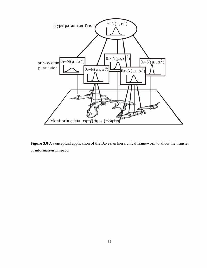
Figure 3.8 A conceptual application of the Bayesian hierarchical framework

to allow the transfer of information in space...................................................83

Figure 3.9 Scenario C. The relative difference between posterior estimates

of the mean values and standard deviations of the hyperparameters

and the system specific parameters..................................................................84

VII

 

List of Appendices

Appendix A NPZD model structure.................................................................................99

Figure A1 The phosphate-detritus-phytoplankton-zooplankton model structure...99

Table A1 The specific functional forms of the NPZD eutrophication model.......100

Appendix B WinBUGS code for the Bayesian Hierarchical model...............................101

Appendix C Posterior estimates for Bayesian Hierarchical Models..............................107

Table C1 Posterior estimates of the model stochastic nodes against three

datasets representing oligo-, meso-, and eutrophic conditions..............107

Table C2 Scenario A. Posterior parameter distributions.......................................108

Table C3 Scenario B. Posterior parameter distributions.......................................109

Table C4 Scenario D. Posterior parameter distributions......................................110

VIII

 

Glossary of Terms Bayes’ Theorem: is a theorem of probability theory originally stated by the Reverend

Thomas Bayes. The theorem relates the conditional and marginal probability distributions

of random variables, and tells how to update or revise beliefs in the light of new evidence

from the study system.

Bayesian Inference: is a statistical approach in which all forms of uncertainty are

expressed in terms of probability, and concerns with the consequences of modifying our

previous beliefs as a result of receiving new data. In the inference process, Bayes'

Theorem is applied to obtain a posterior probability for a specific hypothesis, which

considers both the prior probability and the observations from the study system.

Convergence: is the point in which MCMC sampling techniques eventually reach a

stationary distribution. From this point on, the MCMC scheme moves around this

distribution.

Credible Interval: is a posterior probability interval of a parameter or a model output.

Credible intervals are the Bayesian counterparts of the confidence intervals used in

frequentist statistics.

Likelihood Function: is a conditional function [p(y|θ)] considered as a function of its

second argument (θ, model parameters) with its first argument (y, the data) held fixed.

The likelihood function indicates how likely a particular population (model parameter

set) can produce an observed sample.

Model Calibration: Calibration is the procedure by which the modeler attempts to find

the best fit between computed and observed data by adjusting model parameters.

Markov chain Monte Carlo (MCMC) methods: are a class of algorithms for sampling

from probability distributions based on the construction of a Markov chain that has the

desired distribution as its stationary distribution. This procedure is used to generate a

IX

 

X

 

sequence of samples from a probability distribution that is difficult to be directly

sampled.

Metropolis-Hastings Algorithm: is a rejection sampling algorithm, which generates a

random walk using a proposal density and contains a method for rejecting proposed steps.

It is one algorithm of Markov chain Monte Carlo methods.

NPZD model: model consists of four state variables: nutrient (N) (phosphate, PO43-),

phytoplankton (P), zooplankton (Z), and detritus (D)

Over relaxation: At each MCMC iteration, a number of candidate samples are generated

and one that is negatively correlated with the current value is selected. The time per

iteration will be increased, but the within-chain correlations should be reduced and hence

less iteration may be necessary.

Posterior Distribution: is the conditional probability of a random event or an uncertain

proposition, and it is assigned when the relevant evidence from the study system is taken

into account.

Prior Distribution: is a marginal probability and interpreted as a description of what is

known about a variable in the absence of evidence from the study system.

Runge-Kutta Method: is a family of implicit and explicit iterative methods for the

numerical approximation of solutions of ordinary differential equations.

Sensitivity Analysis: is the process by which the modeler attempts to evaluate the model

sensitivity to the parameters selected, the forcing functions, or the state-variable

submodels.

Chapter 1: Introduction

The importance of investigating the effects of uncertainty on mathematical model

predictions has been extensively highlighted in the modelling literature. Nonetheless, in a

recent meta-analysis, Arhonditsis and Brett (2004) showed that the large majority of the

aquatic biogeochemical models published over the last decade did not properly assess

prediction error and reliability of the critical planning information generated by the

models. Thorough quantification of model sensitivity to parameters, forcing functions

and state variable submodels, was only reported in 27.5% of the studies, while 45.1% of

the published models did not report any results of uncertainty/sensitivity analysis. The

question of model credibility is important because models are used to identify polluters,

to direct the use of research dollars, and to determine management strategies that have

considerable social and economic implications. Erroneous model outputs and failure to

account for uncertainty could produce misleading results and misallocation of limited

resources during the costly implementation of alternative environmental management

schemes. For better model-based decision making, the uncertainty in model projections

must be reduced, or at least explicitly acknowledged, and reported in a straightforward

way that can be easily used by policy planners and decision makers.

Another problematic aspect of the current modelling practice is that the usual

calibration methods do not address the well-known equifinality (poor model

identifiability), where several distinct choices of model inputs lead to the same model

outputs (many sets of parameters fit the data about equally well). A main reason for the

equifinality problem is that the ecological processes/causal mechanisms used for

1

 

understanding how the system works internally is of substantially higher order than what

can be externally observed. However, having a model that realistically reflects the natural

system dynamics is particularly important when the model is intended for making

predictions in the extrapolation domain, i.e., predict future conditions significantly

different from those used to calibrate the mode. For example, when a water quality model

does not operate with realistic relative/absolute magnitudes of biological rates and

transport processes, even if the fit between model outputs and observations is satisfactory

(“good results for the wrong reasons”), its credibility to provide predictions about how

the system will respond under different external nutrient loading conditions is very

limited. In this case, the application of mathematical models for extrapolative tasks is “an

exercise in prophecy” rather than scientific action based on robust prognostic tools.

Another problem that modellers do not always acknowledge is that the conventional

model calibration, may provide the best fit of model input parameters to the dataset

available at the moment, but it is specific to the given dataset at hand. As new data

become available, the model should be recalibrated and in the common calibration

practice there is no way of considering previous results. In this sense, we do not update

previous knowledge about model input parameters, but rather we make the models

dataset-specific.

The first part of this dissertation (Chapter 2) aims to attain effective model

calibration and rigorous uncertainty assessment by integrating complex mathematical

modeling with Bayesian analysis. We used a complex aquatic biogeochemical model that

simulates multiple elemental cycles (org. C, N, P, Si, O), multiple functional

phytoplankton (diatoms, green algae and cyanobacteria) and zooplankton (copepods and

cladocerans) groups. The Bayesian calibration framework is illustrated using three

2

 

synthetic datasets that represent oligo-, meso- and eutrophic lake conditions. Scientific

knowledge, expert judgment, and observational data were used to formulate prior

probability distributions and characterize the uncertainty pertaining to a subset of the

model parameters, i.e., a vector comprising the 35 most influential parameters based on

an earlier sensitivity analysis of the model. The study also underscores the lack of perfect

simulators of natural system dynamics using a statistical formulation that explicitly

accounts for the discrepancy between mathematical models and environmental systems.

The analysis also aimed to illustrate how the Bayesian parameter estimation can be used

for assessing the exceedance frequency and confidence of compliance of different water

quality criteria. The proposed methodological framework can be very useful in the

policy-making process and can facilitate environmental management decisions in the

Laurentian Great Lakes region.

The second part of this dissertation (Chapter 3) presents a Bayesian hierarchical

formulation for simultaneously calibrating aquatic biogeochemical models at multiple

systems (or sites of the same system) with differences in their trophic conditions, prior

precisions of model parameters, available information, measurement error or inter-annual

variability. Model practitioners increasingly place emphasis on rigorous quantitative error

analysis in aquatic biogeochemical models and the existing initiatives range from the

development of alternative metrics for goodness of fit, to data assimilation into

operational models, to parameter estimation techniques. However, the treatment of error

in many of these efforts is arguably selective and/or ad hoc. A Bayesian hierarchical

framework enables the development of robust probabilistic analysis of error and

uncertainty in model predictions by explicitly accommodating measurement error,

parameter uncertainty, and model structure imperfection. Our statistical formulation also

3

 

explicitly considers the uncertainty in model inputs (model parameters, initial

conditions), the analytical/sampling error associated with the field data, and the

discrepancy between model structure and the natural system dynamics (e.g., missing key

ecological processes, erroneous formulations, misspecified forcing functions). The

Bayesian hierarchical approach allows overcoming problems of insufficient local data by

“borrowing strength” from well-studied sites and this feature will be highly relevant to

conservation practices of regions with a high number of freshwater resources for which

complete data could never be practically collected.

4

 

Chapter 2: Predicting the Frequency of Water Quality

Standard Violations Using Bayesian Calibration of

Eutrophication Models 1

2.1 Introduction

In his 2006 review paper, D.W. Schindler highlighted the cultural eutrophication

as one of the preeminent threats to the integrity of freshwater ecosystems worldwide. He

also emphatically argued that our current understanding and management of

eutrophication has evolved from simple control of point and non-point nutrient sources to

the explicit recognition that it often stems from the cumulative effects of the human

activities on climate, global element cycles, land use, and fisheries. Therefore, alleviating

eutrophication problems often involves complex policy decisions aiming to protect the

functional properties of the freshwater ecosystem community as well as to restore many

of the features of the surrounding watershed. In the Great Lakes region, the growing

appreciation of the complexity pertaining to eutrophication control and the need for

addressing the combined effects of a suite of tightly intertwined stressors has sparked

considerable confusion and disagreements (Hartig et al. 1998, Bowerman et al. 1999).

Much of this controversy has arisen as to whether the Great Lakes Water Quality

Agreement is a thrust for improving water quality or for maintaining ecosystem integrity,

and the proposed transition from the Water Quality/Fisheries Exploitation paradigms into

the Ecosystem Management paradigm has been repeatedly debated in the literature

(Bowerman et al. 1999, Minns and Kelso 2000). The defenders of the traditional

5

 

1 In press: J. Great Lakes Res. 2008

paradigms have argued that the shift of focus from water quality to ecosystem

management has also been accompanied by a shift from the traditional identification of

simple cause–effect relationships to a multi-causal way of thinking to accommodate the

complexity of ecosystems. In this context, the crux of the problem is that the ecological

complexity along with the underlying uncertainty can be a major impediment for deriving

the straightforward scientific answers required from the regulatory agencies to implement

the provisions of the Great Lakes Water Quality Agreement (Bowerman et al. 1999,

Krantzberg 2004).

Aside from the environmental thinking, the emergence of the ecosystem approach

has also pervaded the contemporary mathematical modeling practice, increasing the

demand for more complex ecosystem models. Earlier eutrophication modeling studies in

the Great Lakes provided long-term forecasts and insightful retrospective analysis using

as foundation the interplay among nutrient loading, hydrodynamics, phytoplankton

response, and sediment oxygen demand (Bierman and Dolan 1986, Lam et al. 1987a,

DiToro et al. 1987). Yet, the current challenges make compelling the development of

more realistic platforms (i) to elucidate causal mechanisms, complex interrelationships,

direct and indirect ecological paths of the Great Lakes basin ecosystem; (ii) to examine

the interactions among the various stressors (e.g., climate change, urbanization/land-use

changes, alternative management practices, invasion of exotic species); and (iii) to assess

their potential consequences on the lake ecosystem functioning (e.g., food web dynamics,

benthic-pelagic coupling, fish communities) (Mills et al. 2003, Leon et al. 2005). In this

regard, a characteristic example is the integrated eutrophication-zebra mussel

bioenergetic model developed for identifying the factors that promote the re-occurrence

of Microcystis blooms in the Saginaw Bay, Lake Huron (Bierman et al. 2005). It was

6

 

shown that the zebra mussels through selective cyanobacteria rejection, increased

sediment-water phosphorus fluxes can cause structural shifts in the phytoplankton

community, and the impact of these perturbations varies depending on the magnitude of

the zebra mussel densities and their distribution among different age groups. The

Bierman et al. (2005) study is an example of how the increase of the articulation level of

our mathematical models allows performing experiments that are technologically or

economically unattainable by other means, thereby gaining insights into the direct and

synergistic effects induced from the multitude of stressors on the various lake ecosystem

components.

While the development of more holistic modeling constructs is certainly the way

forward, the question arising is: do we have the knowledge to parameterize or even to

mathematically depict the new biotic relationships and their interactions with the abiotic

environment? More importantly, how reliable are the long-term projections generated

from the current generation of mathematical models? Our experience is that the

performance of existing mechanistic biogeochemical models declines as we move from

physical-chemical to biological components of aquatic ecosystems (Arhonditsis and Brett

2004). Because of the still poorly understood ecology, we do not have robust

parameterizations to support predictions in a wide range of spatiotemporal domains

(Anderson 2005). Despite the repeated efforts to explicitly treat multiple biogeochemical

cycles, to increase the functional diversity of biotic communities, and to refine the

mathematical description of the higher trophic levels, modelers still haven’t gone beyond

the phase of identifying the unforeseeable ramifications and the challenges that we need

to confront so as to strengthen model foundation (Anderson 2006). Furthermore, the

additional model complexity will increase the disparity between what ideally we want to

7

 

learn (internal description of the system and model endpoints) and what can realistically

be observed, thereby reducing our ability to properly constrain the model parameters

from observations (Denman 2003). The poor model identifiability undermines the

predictive power of our models and their ability to support environmental management

decisions (Arhonditsis et al. 2006). Thus, the most prudent strategy is to incorporate

complexity gradually and this process should be accompanied by critical evaluation of

the model outputs; the latter concern highlights the central role of uncertainty analysis.

Uncertainty analysis of mathematical models has received considerable attention

in aquatic ecosystem research, and there have been several attempts to rigorously address

issues pertaining to model structure and input error (Beck 1987, Reichert and Omlin

1997, Stow et al. 2007). In this direction, Arhonditsis et al. (2007) recently introduced a

Bayesian calibration scheme using intermediate complexity mathematical models (4-8

state variables) and statistical formulations that explicitly accommodate measurement

error, parameter uncertainty, and model structure imperfection. The Bayesian calibration

methodology offers several technical advances, such as alleviation of the identification

problem, sequential updating of the models, realistic uncertainty estimates of ecological

predictions, and ability to obtain weighted averages of the forecasts from different

models, that can be particularly useful for environmental management (Arhonditsis et al.

2007, 2008a, b). Nonetheless, the capacity of this approach to be coupled with complex

mathematical models has not been demonstrated yet and recent studies have cautioned

that this modeling framework will possibly require substantial modifications to

accommodate highly multivariate outputs (Arhonditsis et al. 2008b).

In this paper, our main objective is to integrate the Bayesian calibration

framework with a complex aquatic biogeochemical model that simulates multiple

8

 

elemental cycles (org. C, N, P, Si, O), multiple functional phytoplankton (diatoms, green

algae and cyanobacteria) and zooplankton (copepods and cladocerans) groups. Because

the model structure and complexity is suitable for addressing a variety of eutrophication-

related problems (chlorophyll a, water transparency, cyanobacteria dominance, hypoxia),

our presentation is highly relevant to the Great Lakes modeling practice. This illustration

is based on three synthetic datasets representing oligo-, meso- and eutrophic lake

conditions. Our analysis also shows how the Bayesian parameter estimation can be used

for assessing the exceedance frequency and confidence of compliance of different water

quality criteria. We conclude by pinpointing some of the anticipated benefits from the

proposed approach, such as the assessment of uncertainty in model predictions and

expression of model outputs as probability distributions, the optimization of the sampling

design of monitoring programs, and the alignment with the policy practice of adaptive

management, which can be particularly useful for stakeholders and policy makers when

making decisions for sustainable environmental management in the Laurentian Great

Lakes region.  

 

2.2 Methods

2.2.1 Model Description

Model spatial structure and forcing functions: The spatial structure of the model

is simpler than the two-compartment vertical system of the original model application in

Lake Washington (Arhonditsis and Brett 2005a, b). We considered a single compartment

model representing the lake epilimnion, whereas the hypolimnion was treated as

boundary conditions to emulate mass exchanges across the thermocline. The external

9

 

forcing encompasses river inflows, precipitation, evaporation, solar radiation, water

temperature, and nutrient loading. The reference conditions for our analysis correspond to

the average epilimnetic temperature, solar radiation, vertical diffusive mixing, hydraulic

and nutrient loading in Lake Washington (Arhonditsis and Brett 2005b, Brett et al. 2005).

The hydraulic renewal rate in our hypothetical system is 0.384 year-1. The fluvial and

aerial total nitrogen inputs are 1114 × 103 kg year-1, and the exogenous total phosphorus

loading contributes approximately 74.9 × 103 kg year-1. The exogenous total organic

carbon supplies in the system are 6685 × 103 kg year-1. In our analysis, the average input

nutrient concentrations for the oligo-, meso-, and eutrophic environments correspond to

50 (2.9 mg TOC/L, 484 μg TN/L and 32.5 μg TP/L), 100 (5.8 mg TOC/L, 967 μg TN/L

and 65 μg TP/L), and 200% (11.6 mg TOC/L, 1934 μg TN/L and 130 μg TP/L) of the

reference conditions, respectively. Based on these nutrient loading scenarios, the model

was run using the calibration vector presented in Arhonditsis and Brett (2005a; see their

Appendix B for parameter definitions and calibration values). The simulated monthly

averages provided the mean values of normal distributions with standard deviations

assigned to be 15 % of the monthly values for each state variable; a fraction that

comprises both analytical error and inter-annual variability at the deeper (middle)

sections of the lake. These distributions were then sampled to generate the oligo-, meso-

and eutrophic datasets used for the Bayesian model calibration.

Plankton community structure: The ecological submodel consists of 24 state

variables and simulates five elemental cycles (organic C, N, P, Si, O) as well as three

phytoplankton (diatoms, green algae and cyanobacteria) and two zooplankton (copepods

and cladocerans) groups (Arhonditsis and Brett 2005a, b). The three phytoplankton

functional groups differ with regards to their strategies for resource competition

10

 

(nitrogen, phosphorus, light, temperature) and metabolic rates as well as their

morphological features (settling velocity, shading effects) (Fig. 2.1a). Phytoplankton

growth temperature dependence has an optimum level and is modeled by a function

similar to a Gaussian probability curve (Cerco and Cole, 1994). Phosphorus and nitrogen

dynamics within the phytoplankton cells account for luxury uptake, and phytoplankton

uptake rates depend on both intracellular and extracellular nutrient concentrations

(Schladow and Hamilton 1997, Arhonditsis et al. 2002). We used Steele’s equation to

describe the relationship between photosynthesis and light intensity along with Beer’s

law to scale photosynthetically active radiation to depth (Jassby and Platt 1976). Diatoms

are modeled as r-selected organisms with high maximum growth rates and higher

metabolic losses, strong phosphorus and weak nitrogen competitors, lower tolerance to

low light availability, low temperature optima, silica requirements, and high sinking

velocities. By contrast, cyanobacteria are modeled as K-strategists with low maximum

growth and metabolic rates, weak P and strong N competitors, higher tolerance to low

light availability, low settling velocities, and high temperature optima. The

parameterization of the third functional group (labelled as “Green Algae”) aimed to

provide an intermediate competitor and more realistically depict the continuum between

diatom- and cyanobacteria-dominated phytoplankton communities.

The two zooplankton functional groups (cladocerans and copepods) differ with

regards to their grazing rates, food preferences, selectivity strategies, elemental somatic

ratios, vulnerability to predators, and temperature requirements (Arhonditsis and Brett

2005a, b). Cladocerans are modeled as filter-feeders with an equal preference among the

four food-types (diatoms, green algae, cyanobacteria, detritus), high maximum grazing

rates and metabolic losses, lower half saturation for growth efficiency, high temperature

11

 

optima and high sensitivity to low temperatures, low nitrogen and high phosphorus

content. In contrast, copepods are characterized by lower maximum grazing and

metabolic rates, capability of selecting on the basis of food quality, higher feeding rates

at low food abundance, slightly higher nitrogen and much lower phosphorus content,

lower temperature optima with a wider temperature tolerance. Fish predation on

cladocerans is modeled by a sigmoid function, while a hyperbolic form is adopted for

copepods (Edwards and Yool 2000). Both forms exhibit a plateau at high zooplankton

concentrations representing satiation of the fish predation, e.g., the fish can only process

a certain number of food items per unit time or there is a maximum limit on predator

density caused by direct interference among the predators themselves. The S-shaped

curve, however, is more appropriate for reproducing the tight connection between

planktivorous fish and large Daphnia adults at higher zooplankton densities, due to fish

specialisation (learning ability of fish to capture large animals) or lack of escape

behaviour of the prey (Lampert and Sommer 1997).

Carbon cycle: The inorganic carbon required for algal photosynthesis is assumed

to be in excess and thus is not explicitly modeled. Dissolved organic carbon (DOC) and

particulate organic carbon (POC) are the two carbon state variables considered by the

model (Fig. 2.1b). Phytoplankton basal metabolism, zooplankton basal metabolism and

egestion of excess carbon during zooplankton feeding release particulate and dissolved

organic carbon in the water column. A fraction of the particulate organic carbon

undergoes first-order dissolution to dissolved organic carbon, while another fraction

settles to the sediment. Particulate organic carbon is grazed by zooplankton (detrivory),

dissolved organic carbon is lost through a first-order denitrification and respiration during

heterotrophic activity.

12

 

Nitrogen cycle: There are four nitrogen forms considered by the model: nitrate

(NO3-), ammonium (NH4

+), dissolved organic nitrogen (DON), particulate organic

nitrogen (PON) (Fig. 2.1c). Both ammonium and nitrate are utilized by phytoplankton

during growth and Wroblewski’s model (1977) was used to describe ammonium

inhibition of nitrate uptake. Phytoplankton basal metabolism, zooplankton basal

metabolism and egestion of excess nitrogen during zooplankton feeding release

ammonium and organic nitrogen in the water column. A fraction of the particulate

organic nitrogen hydrolyzes to dissolved organic nitrogen. Dissolved organic nitrogen is

mineralized to ammonium. In an oxygenated water column, ammonium is oxidized to

nitrate through nitrification and its kinetics are modeled as a function of available

ammonium, dissolved oxygen, temperature and light (Cerco and Cole 1994, Tian et al.

2001). During anoxic conditions, nitrate is lost as nitrogen gas through denitrification.

Phosphorus cycle: Three phosphorus state variables were considered in the

model: phosphate (PO43-), dissolved organic phosphorus (DOP), and particulate organic

phosphorus (POP) (Fig. 2.1d). Phytoplankton uptakes phosphate and redistributes the

three forms of phosphorus through basal metabolism. Zooplankton basal metabolism and

egestion of excess phosphorus during feeding release phosphate and dissolved/particulate

organic phosphorus. Particulate organic phosphorus can be hydrolyzed to dissolved

organic phosphorus, and another fraction settles to the sediment. Dissolved organic

phosphorus is mineralized to phosphate through a first-order reaction.

2.2.2 Bayesian Framework

i) Statistical formulation: Our presentation examines a statistical formulation

founded on the assumption that the eutrophication model is an imperfect simulator of the

13

 

environmental system and the model discrepancy is invariant with the input conditions,

i.e., the difference between model and lake dynamics was assumed to be constant over

the annual cycle for each state variable. This formulation aims to combine field

observations with simulation model outputs to update the uncertainty of model

parameters, and then use the calibrated model to give predictions (along with uncertainty

bounds) of the natural system dynamics. An observation i for the state variable j, yij, can

be described as:

yij = f(θ, xi, y0) + δj + εij, i = 1, 2, 3,…..n and j = 1,…,m (2-1)

g(θ, xi, y0, δj) ~ N(f(θ, xi, y0),σj2)

where f(θ, xi, y0) denotes the eutrophication model, xi is a vector of time dependent

control variables (e.g., boundary conditions, forcing functions) describing the

environmental conditions, the vector θ is a time independent set of the calibration model

parameters, y0 corresponds to the vector of the concentrations of the twenty four state-

variables at the initial time point t0 (initial conditions), the stochastic term δj accounts for

the discrepancy between the model and the natural system, εij denotes the observation

(measurement) error that is usually assumed to be independent and identically distributed

following a Gaussian distribution, and g(θ, xi, y0, δj) represents a normally distributed

variable with first and second order moments based on the model predictions and the

time independent model structural error σj2. In this study, as a result of the scheme

followed to generate the three datasets, we assumed a multiplicative measurement error

with standard deviations proportional (15%) to the average monthly values for each state

variable (Van Oijen et al. 2005). With this assumption, the likelihood function (see

Glossary of Terms) will be:

14

 

( ) ( ) ( )[ ] ( )[ ]⎥⎦⎤

⎢⎣⎡ −Σ−−= −

=

−−∏ 01

01

2120 ,,,,

21exp2),,( yxfyyxfyΣπyxθfyp jjTotj

Tjj

m

j

/

Totjn/ θθ

(2-2)

jjTotj εδ Σ+Σ=Σ (2-3)

where m and n correspond to the number of state variables (m = 24) and the number of

observations in time used to calibrate the model (n = 12 average monthly values),

respectively; yj = [y1j,…,ynj]T and fj(θ, x, y0) = [f1j(θ, x1, y0),…, fnj(θ, xn, y0)]T correspond

to the vectors of the field observations and model predictions for the state variable j; Σδj

= In·σj2 corresponds to the stochastic term of the model; and Σεj = In·(0.15) 2·yj

T·yj. In the

context of the Bayesian statistical inference, the posterior density of the parameters θ and

the initial conditions of the twenty four state variables y0 given the observed data y is

defined as:

( ) ( ) ( )( ) ( )

( ) ( ) )()(),,,(∝)()(),,,(

)()(),,,(,, 2

02

020

20

20

20

202

0 σθσθσθσθσθ

σθσθσθ pyppyxfyp

ddydpyppyxfyppyppyxfyp

yyp∫∫∫

=

(2-4)

p(θ) is the prior density of the model parameters θ and p(y0) is the prior density of the

initial conditions of the twenty four state variables y0. In a similar way to the

measurement errors, the characterization of the prior density p(y0) was based on the

assumption of a Gaussian distribution with a mean value derived from the January

monthly averages during the study period and standard deviation that was 15% of the

mean value for each state variable j; the prior densities p(σj2) were based on the conjugate

inverse-gamma distribution (Gelman et al. 1995). Thus, the resulting posterior

distribution for θ, y0, and σ2 is:

15

 

( ) ( ) ( )[ ] ( )[ ]⎥⎦⎤

⎢⎣⎡ −Σ−−∝ −

=

−−∏ 01

01

21220 ,,,,

21exp2,, yxfyyxfyΣπyyp jjTotj

Tjj

m

j

/

Totjn/ θθσθ

( ) [ ] [ ]⎥⎦⎤

⎢⎣⎡ −Σ−−× −

=

−− ∏ 01

01

212 loglog21exp12 θθθθ

θ θθT

l

k k

/l/ Σπ

( ) [ ] [ ]⎥⎦⎤

⎢⎣⎡ −Σ−−× −−−

myT

m

/

ym/ yyyyΣπ 00

1000

21

02

21exp2

∏=

+− −Γ

×m

j j

jj

j

jj j

12

)1(2 )exp()( σ

βσ

αβ α

α

(2-5)

where l is the number of the model parameters θ used for the model calibration (l = 35);

θ0 indicates the vector of the mean values of θ in logarithmic scale; Σθ = Il·σθT·σθ and σθ =

[σθ1,…, σθl]T corresponds to the vector of the shape parameters of the l lognormal

distributions (standard deviation of log θ); the vector y0m = [y1,1,…, y1,24]T corresponds to

the January values of the twenty four state variables; Σy0 = Im·(0.15) 2·y0mT·y0m; αj (= 0.01)

and βj (= 0.01) correspond to the shape and scale parameters of the m non-informative

inverse-gamma distributions used in this analysis.

ii) Prior parameter distributions: The calibration vector consists of the 35 most

influential parameters as identified from an earlier sensitivity analysis of the model

(Arhonditsis and Brett 2005a). The prior parameter distributions reflect the existing

knowledge (field observations, laboratory studies, literature information and expert

judgment) on the relative plausibility of their values. For example, based on the previous

characterization of the three functional groups, we assigned probability distributions that

represent their differences in growth and storage strategies, basal metabolism, nitrogen

and phosphorus kinetics, light and temperature requirements, and settling velocity. In this

study, we used the following protocol to formulate the parameter distributions: i) we

identified the global (not the group-specific) minimum and maximum values for each

16

 

parameter from the pertinent literature; ii) we partitioned the original parameter space

into three subregions reflecting the functional properties of the phytoplankton groups;

and then iii) we assigned lognormal distributions parameterized such that 98% of their

values were lying within the identified ranges (Steinberg et al. 1997). The group-specific

parameter spaces were also based on the calibration vector presented during the model

application in Lake Washington (Arhonditsis and Brett 2005a). For example, the

identified range for the maximum phytoplankton growth rate was 1.0-2.4 day-1, while the

three subspaces were 2.2 ± 0.2 day-1 for diatoms (calibration value ± literature range), 1.8

± 0.2 day-1 for greens and 1.3 ± 0.3 day-1 for cyanobacteria. We then assigned lognormal

distributions formulated such that 98% of their values were lying within the specified

ranges, i.e., growthmax(diat) ~ Λ(2.19, 1.040), growthmax(greens) ~ Λ(1.79, 1.049),

growthmax(cyan) ~ Λ(1.26, 1.106). The prior distributions of all the parameters of the model

calibration vector are presented in Table 2.1.

iii) Numerical approximations for posterior distributions: Sequence of

realizations from the posterior distribution of the model were obtained using Markov

chain Monte Carlo (MCMC) simulations (Gilks et al. 1998). We used the general

normal-proposal Metropolis algorithm coupled with an ordered over-relaxation to control

the serial correlation of the MCMC samples (Neal 1998). In this study, we present results

using two parallel chains with starting points: (i) a vector that consists of the mean values

of the prior parameter distributions, and (ii) the calibration vector of the application Lake

Washington. We used 30,000 iterations and convergence was assessed with the modified

Gelman–Rubin convergence statistic (Brooks and Gelman 1998). The accuracy of the

posterior estimates was inspected by assuring that the Monte Carlo error (an estimate of

the difference between the mean of the sampled values and the true posterior mean; see

17

 

Spiegelhalter et al. 2003) for all the parameters was less than 5% of the sample standard

deviation. Our framework was implemented in the WinBUGS Differential Interface

(WBDiff); an interface that allows numerical solution of systems of ordinary differential

equations within the WinBUGS software.

2.3 Results

The MCMC sequences of the three applications of the model converged rapidly

(≈ 5,000 iterations) and the statistics reported were based on the last 25,000 draws by

keeping every 4th iteration (thin = 4). The uncertainty underlying the values of the 35

model parameters after the MCMC sampling is depicted on the respective marginal

posterior distributions (Table 2.1 and Fig. 2.2). Generally, the moments of the posterior

parameter distributions indicate that the knowledge gained for the 35 parameters after the

Bayesian updating of the complex eutrophication model was fairly limited. [It should be

noted that for the sake of consistency all the parameter posteriors were presented as

lognormal distributions, although in several cases the shape is better approximated by a

uniform distribution.] Namely, most of the calibration parameters were characterized by

minor or no shifts of their central tendency relative to the prior assigned values, such as

the half saturation constants for nitrogen uptake (KN(i); i= diatoms, greens, cyanobacteria), the half

saturation constants for grazing (KZ(j); j= cladocerans, copepods), and the half saturation

constants for growth efficiency (ef2(j); j= cladocerans, copepods). Nonetheless, there were

parameters with moderate shifts of their posterior mean values; characteristic examples

were the nitrogen mineralization rate (KNrefmineral) with relative percentage changes of 14,

23, and 11% in the oligo-, meso-, and eutrophic environments, respectively; the light

18

 

attenuation coefficient for chlorophyll (KEXTchla) with 6, 15, and 14% relative changes in

the three nutrient enrichment conditions; settling velocity for diatoms (Vsettling(diat)) with 9,

13, and 7% relative shifts. Furthermore, the vast majority of the posterior standard

deviations increased or remained unaltered relative to the prior assigned values, and

several parameter posteriors were almost uniformly distributed within the specified

ranges prior to the model calibration. Notable exceptions were the dissolution/hydrolysis

rates for particulate carbon (KCrefdissolution), nitrogen (KNrefdissolution), phosphorus

(KPrefdissolution), and silica (KSirefdissolution) with approximately 2-6% relative decrease of the

respective standard deviations. The standard deviation of the diatom settling velocity

(Vsettling(diat)) was also reduced by 3% in the mesotrophic state.

The comparison between the observed and posterior predictive monthly

distributions for the three trophic states indicates that the eutrophication model combined

with the Bayesian calibration scheme provides an accurate representation of the system

dynamics. In the oligotrophic environment, the observed monthly values were included

within the 95% credible intervals of the model predictions throughout the simulation

period, while the median values of model predictions closely matched the observed

patterns (Fig. 2.3). In a similar manner, all the observed values of the dataset representing

the mesotrophic conditions were included within the 95% credible intervals, although the

median model predictions slightly underestimated the spring biomass peaks of three

phytoplankton groups (Fig. 2.4). In the eutrophic scenario, the model closely reproduced

the summer prey-predator oscillations between cladocerans and the three phytoplankton

groups and also accurately simulated the nutrient dynamics, i.e., total nitrogen, nitrate,

ammonium, total phosphorus, and phosphate (Fig. 2.5). However, the central tendency

and uncertainty bounds of the copepod biomass predictive distribution failed to capture

19

 

the late-spring peak, while the upper (97.5%) and lower (2.5%) uncertainty boundaries

showed convexo-convex shape during the same period.

The model performance for each trophic state was evaluated by three measures of

fit: root mean squared error (RMSE), relative error (RE) and average error (AE) (Table

2.2). These comparisons aimed to assess the goodness-of-fit between the medians of the

predictive distributions and the observed values. The application of the model to the

oligotrophic environment was characterized by the lowest RE values (1.19-10.6%), while

the mesotrophic and eutrophic scenarios resulted in moderate (3.37-13.6%), and

relatively larger RE values (6.03-21.2%), respectively. We also highlight the fairly high

RE values for cyanobacteria and copepod biomass in the eutrophic environment, whereas

total nitrogen and dissolved oxygen had consistently low REs in the three nutrient

loading scenarios. The average error is a measure of aggregate model bias, though values

near zero can be misleading because negative and positive discrepancies can cancel each

other. In most cases, we found that the medians of the state variable predictive

distributions underestimated the observed levels, whereas dissolved oxygen was

overestimated with an AE value of 0.482, 0.356, and 0.628 mg L-1 in the oligo-, meso-,

and eutrophic environment, respectively. The root mean square error is another measure

of the model prediction accuracy that overcomes the shortcoming of the average error by

considering the magnitude rather than the direction of each difference. The RMSE for the

copepod biomass increased across the trophic gradient examined from 5.19 μg C L-1 in

the oligotrophic to 13.2 and 48.3 μg C L-1 in the meso- and eutrophic datasets,

respectively. We also note the approximately 0.5 μg chla L-1 mean discrepancy between

the predictive medians and the observed cyanobacteria biomass values.

20

 

The seasonally invariant error terms (σj) delineate a constant zone around the

model predictions for the 24 state variables that accounts for the discrepancy between the

model simulation and the natural system dynamics (Table 2.3). The majority of the

discrepancy terms increased as we move from the oligotrophic to the eutrophic state,

providing evidence that these terms play an important role in accommodating the

increased intra-annual variability of the meso- and eutrophic datasets. On the other hand,

the error terms associated with the phytoplankton intracellular nutrient storage (e.g., σN,

P(i); i= diatoms, greens, cyanobacteria, and σSi(diatoms)) were characterized by similar mean and

standard deviation values across the trophic gradient examined. Finally, high coefficients

of variation (standard deviation/mean) were found for the dissolved oxygen, dissolved

organic carbon, and dissolved silica error terms.

Exceedance frequency and confidence of compliance with water quality

standards: The MCMC posterior samples were also used to examine the exceedance

frequency and confidence of compliance with different water quality standards under the

three nutrient loading scenarios. For illustration purposes, we selected three water quality

variables of management interest, i.e., chlorophyll a concentration, total phosphorus, and

percentage cyanobacteria contribution to the total phytoplankton biomass, and then

specified their threshold values (numerical criteria) at 5 μg Chl a L-1, 25 μg TP L-1, and

30%, respectively. For each iteration, we calculated the monthly predicted values and the

corresponding probabilities of exceeding the three water quality criteria. The latter

probabilities were calculated as follows:

( ) ( )⎟⎟⎠

⎞⎜⎜⎝

⎛ −′−=′>=

εσδθ

θ,,,

1,,| 00

yxgcFyxccPp (2-6)

21

 

where p is the probability of the response variable exceeding a numerical criterion c’,

given values of θ, x, and y0, σε is the measurement error/within-month variability, and F(.)

is the value of the cumulative standard normal distribution. The monthly predicted values

along with the calculated exceedance frequencies were then averaged over the summer

stratified period (June-September). The distribution of these statistics across the posterior

space (12,500 MCMC samples) can be used to assess the expected exceedance frequency

and the confidence of compliance with the three water quality standards, while

accounting for the uncertainty that stems from the model parameter uncertainty. It should

be noted that the exceedance frequency is not necessarily normally distributed, especially

since this value is calculated as the average over the stratified period (Borsuk et al. 2002).

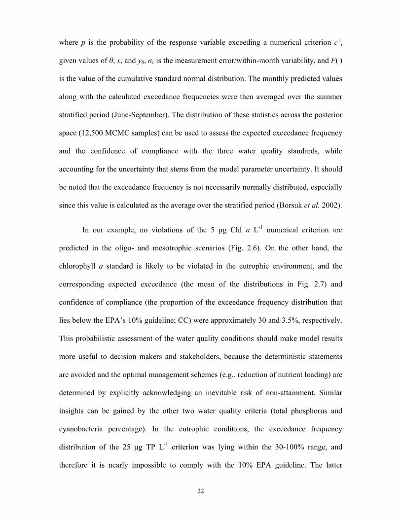
In our example, no violations of the 5 μg Chl a L-1 numerical criterion are

predicted in the oligo- and mesotrophic scenarios (Fig. 2.6). On the other hand, the

chlorophyll a standard is likely to be violated in the eutrophic environment, and the

corresponding expected exceedance (the mean of the distributions in Fig. 2.7) and

confidence of compliance (the proportion of the exceedance frequency distribution that

lies below the EPA’s 10% guideline; CC) were approximately 30 and 3.5%, respectively.

This probabilistic assessment of the water quality conditions should make model results

more useful to decision makers and stakeholders, because the deterministic statements

are avoided and the optimal management schemes (e.g., reduction of nutrient loading) are

determined by explicitly acknowledging an inevitable risk of non-attainment. Similar

insights can be gained by the other two water quality criteria (total phosphorus and

cyanobacteria percentage). In the eutrophic conditions, the exceedance frequency

distribution of the 25 μg TP L-1 criterion was lying within the 30-100% range, and

therefore it is nearly impossible to comply with the 10% EPA guideline. The latter

22

 

conclusion can also be drawn with regards to the 30% cyanobacteria biomass criterion,

although in this case a fairly low confidence of compliance also characterizes the

mesotrophic state. Analogous statements can be made with other model endpoints of

management interest, such as the spatiotemporal dissolved oxygen levels in systems

experiencing problems of prolonged hypoxia (e.g., Lake Erie).

2.4 Discussion

The water quality management usually relies on mathematical models with strong

mechanistic basis, as this improves the confidence in predictions made for a variety of

conditions. From an operational standpoint, the interpretation of model results should

explicitly consider two sources of model error, i.e., the observed variability that is not

explained by the model and the uncertainty arising from the model parameters and/or the

misspecification of the model structure (Arhonditsis et al. 2007, Stow et al. 2007). In this

study, we illustrated a methodological framework that can accommodate rigorous and

complete error analysis, thereby allowing for the direct assessment of the frequency of

water quality standard violations along with the determination of an appropriate margin

of safety (Borsuk et al. 2002). The latter term refers to the probability distribution of the

predicted exceedance probabilities and represents the degree of confidence that the true

value of the violation frequency is below a specified value (Wild et al. 1996, McBride

and Ellis 2001). The presentation of the model outputs as probabilistic assessment of

water quality conveys significantly more information than the point predictions and is

conceptually similar to the percentile-based standards proposed by the EPA-guidelines

(Office of Water 1997). In this regard, our analysis also builds upon the

23

 

recommendations of an earlier modeling work by Lam et al. (1987b), which advocated

the use of probability indicators in water quality assessment in the Great Lakes area,

recognizing the importance of the variability pertaining to nutrient loading and weather

conditions. This type of probabilistic information is certainly more appealing to decision

makers and stakeholders, as it acknowledges the knowledge gaps, the inherent

uncertainty, and the interannual variability typically characterizing freshwater ecosystems

(Ludwig 1996). The latter feature is particularly important in the most degraded and

highly variable nearshore zones or enclosed bays/harbours in the Great Lakes. These

areas are transitional zones in that they receive highly polluted inland waters from

watersheds with significant agricultural, urban and/or industrial activities while mixing

with offshore waters having different biological and chemical characteristics. Generally,

we believe that the Bayesian calibration presented herein can be particularly useful in the

context of the Great Lakes modeling, although our analysis highlighted several technical

features that need to be acknowledged so as to put this framework into perspective.

As demonstrated in several recent studies (Arhonditsis et al. 2007, 2008a, b), the

inclusion of the monthly invariant stochastic terms that account for model structure

imperfection resulted in a close reproduction of the epilimnetic patterns. Even though the

median model predictions tend to slightly underestimate the spring plankton bloom, all

the observed monthly values of the datasets representing the three trophic states were

included within the 95% credible intervals. It is important to note, however, that the

updating of the model mainly changed the discrepancy error terms instead of the model

input parameters; namely, the terms that reflect the model inadequacy and not the

mathematical model itself were used to accommodate the temporal variability across the

trophic gradient examined. The latter result does not fully satisfy the basic premise of our

24

 

framework to attain realistic forecasts while gaining insight into the ecological structure

(e.g., cause-effect relationships, feedback loops) underlying system dynamics. Similar

results were also reported in an earlier exercise of sequential model updating (Arhonditsis

et al. 2008a), but here the increased complexity of the model has further reduced the

updating of the posterior parameter distributions. A more parsimonious statistical

configuration of the model will assume a “perfect” model structure, i.e., the difference

between model and lake dynamics is only caused by the observation/measurement error

(Higdon et al. 2004, Arhonditsis et al. 2007). Applications of this statistical formulation

resulted in narrow-shaped posterior parameter distributions but also in substantial

misrepresentation of the calibration dataset (Arhonditsis et al. 2008a, b). Both features

were attributed to the overconditioning of the parameter estimates because the lack of

potential for model error tends to overestimate the information content of the

observations (Beven 2006). These contradictory results highlight the pivotal role of the

assumptions pertaining to model error structure and invite further examination of

statistical formulations that objectively weigh the relative importance of the discrepancy

terms vis-à-vis the model parameters on the calibration results. For example, future

research should evaluate formulations that explicitly consider the dependence patterns of

the error terms in time/space along with the covariance between measurement error and

model structural error (Beven 2006, Arhonditsis et al. 2008b).

The determination of the model structure (and associated parameter values) that

realistically represents the natural system dynamics is the basic foundation for developing

robust prognostic tools (Reichert and Omlin, 1997). However, most of the calibration

schemes in the modeling literature have not adequately addressed the problem of

uncertainty, and sometimes generate more questions than answers. Model calibration is

25

 

mainly presented as an inverse solution exercise (i.e., the data for the model endpoints are

used to learn something about the parameters) or as an exercise for delineating

uncertainty zones around the mean predictions (Beven 1993, Beven 2001). In ecological

modeling, the model parameters correspond to ecological processes for which we usually

have substantial amount of information on the relative plausibility of their values (e.g.,

Jorgensen et al. 1991). Thus, it is a significant omission to ignore this knowledge and

solely let the data to offer insights into the parameter marginal distributions. In this study,

prior information of the magnitudes of ecological processes (based on field observations

from the lake, laboratory studies, literature information, and expert judgment) was used

to formulate probability distributions that reflect the relative likelihood of different values

of the respective model parameters. Earlier studies have indicated that the inclusion of

these informative distributions into the “prior-likelihood-posterior” update cycles of

intermediate complexity models favours solutions that more realistically depict the

internal structure of the system and avoid getting “good results for the wrong reasons”;

the latter finding has been reported even when the mathematical models were coupled

with statistical formulations that explicitly consider discrepancy error terms (Arhonditsis

et al. 2007, 2008a, b). In this analysis, however, the relatively uninformative patterns of

the posterior parameter space suggest that the efficiency of this scheme can be

compromised with complex model structures (≥ 15-20 state variables). Interestingly, our

analysis showed a relatively higher change (central tendency shifts and standard

deviation reductions) of the posterior moments of some parameters associated with the

nutrient recycling in the system, i.e., dissolution and mineralization rates. Despite the

aforementioned role of the model structure error terms and the high dimensional input

space (35 model parameters) of the complex simulation model examined, some of the

parameters representing feedback loops of the system played a somewhat more active

26

 

role during the Bayesian updating process. Finally, the high coefficients of variation for

the DO, DOC, and DSi error terms are indicative of the relatively low intra-annual

variability characterizing these state variables (Arhonditsis et al. 2008a).

Aside from the probabilistic assessment of the water quality conditions, another

benefit of the Bayesian parameter estimation is the alignment with the policy practice of

adaptive management, i.e., an iterative implementation strategy that is recommended to

address the often-substantial uncertainty associated with water quality model forecasts,

and to avoid the implementation of inefficient and flawed management plans (Walters

1986). Adaptive implementation or “learning while doing” supports initial model

forecasts of management schemes with post-implementation monitoring, i.e., the initial

model forecast serves as the Bayesian prior, the post-implementation monitoring data

serve as the sample information (the likelihood), and the resulting posterior probability

(the integration of monitoring and modeling) provides the basis for revised management

actions (Qian and Reckhow 2007). The probabilistic predictions for water quality

variables of management interest (e.g., chlorophyll a, dissolved oxygen) can also be used

to optimize water quality monitoring programs (Van Oijen et al. 2005). For example in

Fig. 2.8, the sections of the system where water quality conditions are more uncertain

(“flat” distributions; C and D in the first map) should be more intensively monitored.

These model predictions form the Bayesian prior which then is integrated (updated) with

additional monitoring data to provide the posterior distribution. Based on the patterns of

the posterior predictive distributions (where the predictive distribution for one site

indicates a “high” probability of non-attaining water quality goals or, alternatively, an

“unacceptably high” variance), we can determine again the optimal sampling design for

water quality monitoring and assess the value of information (value of additional

27

 

monitoring; “Where should additional water quality data collection efforts be

focused?”). The Bayesian inference and decision theory can also provide a coherent

framework for decision making in problems of natural resources management (Dorazio

and Johnson 2003). Management objectives can be evaluated by integrating the

probability of use attainment for a given water quality goal with utility functions that

reflect different socioeconomic costs and benefits. The water quality goals (resulting

from specific management schemes) associated with the highest expected utility might

then be chosen (Dorazio and Johnson 2003).

2.5 Conclusions

We illustrated a novel methodological framework that effectively addresses

several aspects of model uncertainty (model structure, model parameters, initial

conditions, and forcing functions) and explicitly examines how they can undermine the

credibility of model predictions. We also demonstrated how the Bayesian parameter

estimation can be used for assessing the exceedance frequency and confidence of

compliance of different water quality criteria. The present analysis also highlighted the

difficulty in unequivocally dissaggregating the role of the uncertainty in model inputs and

the error associated with the model structure (parameters versus model imperfection error

terms); especially when using complex statistical formulations and models with

multivariate outputs. Generally, our study provides overwhelming evidence that the

coupling of the Bayesian calibration framework with complex overparameterized

simulation models can negate the premise of attaining realistic forecasts while gaining

mechanistic insights into the ecosystem dynamics. Thus, the use of complex models is

28

 

advised only if existing prior information from the system can reasonably constrain the

input parameter space, thereby ensuring model fit that is not founded on uninformative

and/or fundamentally flawed ecological structures (e.g., unrealistic magnitudes of the

various ecological processes). In cases where prior knowledge does not exist, it is advised

to start with intermediate complexity models (4-10 state variables) and then gradually

increase the complexity as more information becomes available (Arhonditsis et al.

2008b).

The latter assertions do not imply that this framework cannot accommodate the

enormous complexity characterizing environmental systems, but rather are an indication

that the rigid structure of complex mathematical models can be replaced by more flexible

modeling tools (e.g., Bayesian networks) with the ability to integrate quantitative

descriptions of ecological processes at multiple scales and in a variety of forms

(intermediate complexity mathematical models, empirical equations, expert judgments),

depending on available information (Borsuk et al. 2004). Regarding the spatial model

resolution, our presentation was based on a single-compartment model for the sake of

simplicity, but it should be acknowledged that the Bayesian framework can be easily

employed with the segmentations of existing Great Lakes models, i.e., 5-10 completely-

mixed boxes (Lam et al. 1987a; DiToro et al. 1987; Bierman et al. 2005). It is expected

though that the use of finer grid resolutions will significantly increase the computation

demands along with the simulation time required. To overcome this impediment, on-

going research should focus on the use of more flexible schemes, such as nested grid

configurations that can reduce the computational time compared to the standard approach

(one fixed grid size) and better capture the interplay between pollutant mixing/dispersion

and food web dynamics in the nearshore areas, while the offshore water dynamics can be

29

 

sufficiently reproduced with coarser spatio-temporal resolution. The patterns of the

posterior uncertainty can then be used to further optimize the spatial model segmentation

(e.g., splitting-up segments with flat posteriors or lumping segments with similar,

narrow-shaped predictions) and avoid overly cumbersome modeling constructs that

profoundly violate the parsimony principle.

Bearing in mind the pending reevaluation of the Great Lakes Water Quality

Agreement, the Great Lakes community -as it did in the 1970s- has the opportunity to set

the standard for the innovative use of mathematical models in support of decision-

making. Despite the unresolved technical issues, we believe that the benefits from the

Bayesian calibration scheme proposed, such as the assessment of uncertainty in model

predictions and expression of model outputs as probability distributions, the alignment

with the policy practice of adaptive management, and the optimization of the sampling

design of monitoring programs can be particularly useful for stakeholders and policy

makers when making decisions for sustainable environmental management in the

Laurentian Great Lakes region.

30

 

Tables

Table 2.1 Prior and posterior parameter distributions in three trophic states: Λ– lognormal distribution, θ ~ Λ(µ*, σ*) is a mathematical expression meaning that θ is lognormally distributed, µ* and σ* correspond to the median and multiplicative standard deviation.

Parameters Prior Oligotrophic Mesotrophic Eutrophic bmref(clad) Λ(0.0495, 1.161) Λ(0.0491, 1.236) Λ(0.0490, 1.239) Λ(0.0491, 1.241) bm ref(cop) Λ(0.0442, 1.181) Λ(0.0441, 1.271) Λ(0.0438, 1.271) Λ(0.0444, 1.265) bmref(cyan) Λ(0.0775, 1.116) Λ(0.0774, 1.168) Λ(0.0789, 1.163) Λ(0.0808, 1.162) bmref(diat) Λ(0.0980, 1.091) Λ(0.0978, 1.144) Λ(0.0951, 1.125) Λ(0.0946, 1.120) bmref(green) Λ(0.0775, 1.116) Λ(0.0760, 1.170) Λ(0.0753, 1.164) Λ(0.0753, 1.163)

ef2(clad) Λ(18.3, 1.123) Λ(18.3, 1.183) Λ(18.3, 1.181) Λ(18.1, 1.183) ef2(cop) Λ(19.4, 1.116) Λ(19.3, 1.174) Λ(19.3, 1.172) Λ(19.4, 1.166)

growthmax(cyan) Λ(1.26, 1.106) Λ(1.29, 1.155) Λ(1.28, 1.158) Λ(1.22, 1.145) growthmax(diat) Λ(2.19, 1.040) Λ(2.23, 1.050) Λ(2.24, 1.049) Λ(2.22, 1.055)

growthmax(greens) Λ(1.79, 1.049) Λ(1.80, 1.070) Λ(1.80, 1.073) Λ(1.81, 1.070) grazingmax(clad) Λ(0.837, 1.080) Λ(0.837, 1.118) Λ(0.839, 1.115) Λ(0.844, 1.121) grazingmax(cop) Λ(0.490, 1.091) Λ(0.489, 1.134) Λ(0.477, 1.125) Λ(0.490, 1.139) KCrefdisslution Λ(0.00200, 2.691) Λ(0.00194, 2.573) Λ(0.00198, 2.588) Λ(0.00206, 2.643)

Keddyref Λ(0.0316, 1.218) Λ(0.0351, 1.277) Λ(0.0325, 1.340) Λ(0.0322, 1.277) KEXTback Λ(0.265, 1.084) Λ(0.256, 1.106) Λ(0.244, 1.075) Λ(0.252, 1.097) KEXTchla Λ(0.0200, 1.347) Λ(0.0187, 1.489) Λ(0.0169, 1.424) Λ(0.0173, 1.452) KN(cyan) Λ(22.9, 1.200) Λ(22.8, 1.308) Λ(22.9, 1.298) Λ(23.0, 1.306) KN(diat) Λ(64.2, 1.069) Λ(64.1, 1.101) Λ(64.1, 1.101) Λ(64.2, 1.101)

KN(greens) Λ(43.9, 1.102) Λ(43.9, 1.151) Λ(43.9, 1.150) Λ(43.7, 1.149) KNrefdisslution Λ(0.00200, 2.691) Λ(0.00201, 2.663) Λ(0.00199, 2.613) Λ(0.00195, 2.594) KNrefmineral Λ(0.00775, 1.503) Λ(0.00884, 1.622) Λ(0.00594, 1.559) Λ(0.00691, 1.716)

KP(cyan) Λ(19.4, 1.116) Λ(19.2, 1.174) Λ(19.7, 1.168) Λ(19.5, 1.174) KP(diat) Λ(5.66, 1.161) Λ(5.28, 1.216) Λ(5.36, 1.226) Λ(5.46, 1.235)

KP(greens) Λ(10.6, 1.128) Λ(10.4, 1.187) Λ(10.3, 1.187) Λ(10.4, 1.188) KPrefdisslution Λ(0.00200, 2.691) Λ(0.00202, 2.604) Λ(0.00198, 2.603) Λ(0.00202, 2.668) KPrefmineral Λ(0.0245, 1.470) Λ(0.0220, 1.644) Λ(0.0235, 1.691) Λ(0.0235, 1.716)

KSi(diat) Λ(40.0, 1.347) Λ(39.7, 1.542) Λ(39.8, 1.536) Λ(39.8, 1.527) KSirefdisslution Λ(0.00200, 2.691) Λ(0.00198, 2.631) Λ(0.00197, 2.613) Λ(0.00194, 2.533)

KZ(clad) Λ(114, 1.058) Λ(114, 1.087) Λ(114, 1.087) Λ(113, 1.085) KZ(cop) Λ(93.8, 1.071) Λ(93.6, 1.104) Λ(94.5, 1.104) Λ(93.3, 1.100) pred1 Λ(0.141, 1.161) Λ(0.139, 1.238) Λ(0.138, 1.233) Λ(0.136, 1.224) pred2 Λ(34.6, 1.266) Λ(36.1, 1.400) Λ(35.5, 1.412) Λ(39.4, 1.330)

Vsettling(cyan) Λ(0.0224, 1.413) Λ(0.0205, 1.590) Λ(0.0224, 1.605) Λ(0.0232, 1.610) Vsettling(diat) Λ(0.316, 1.106) Λ(0.289, 1.112) Λ(0.275, 1.072) Λ(0.293, 1.118)

Vsettling(greens) Λ(0.245, 1.091) Λ(0.237, 1.128) Λ(0.231, 1.108) Λ(0.235, 1.120)

31

 

Table 2.2 Goodness-of-fit statistics for the model state variables in three trophic states*.

Oligotrophic Mesotrophic Eutrophic State Variables RMSE RE AE RMSE RE AE RMSE RE AE

Green Algae Biomass (μg Chl a/L) 0.118 7.03% -0.050 0.223 8.49% -0.092 0.251 7.63% -0.117

Diatom Biomass (μg Chl a/L) 0.307 10.4% -0.139 0.467 13.6% -0.215 0.275 7.17% -0.139

Cyanobacteria Biomass (μg Chl a/L) 0.059 8.26% -0.028 0.235 10.7% -0.082 0.552 12.8% -0.188

Copepod Biomass (μg C/L)

5.19 10.6% -2.00 13.2 12.6% -4.74 48.3 21.2% -15.6

Cladoceran Biomass (μg C/L)

3.41 7.04% -1.62 4.40 5.92% -2.20 8.42 6.03% -4.23

Total Silica (mg Si/L)

0.097 7.50% 0.019 0.136 8.25% -0.0085 0.222 8.61% -0.0030

Total Nitrogen (μg N/L)

4.06 1.19% -2.77 14.4 3.37% -9.48 45.4 7.64% -12.5

Total Phosphorus (μg P/L)

0.627 4.16% -0.350 1.17 4.62% -0.648 4.74 9.81% -1.16

Dissolved Oxygen (mg DO/L)

0.655 4.92% 0.482 0.629 5.04% 0.356 0.763 6.37% 0.628

* RMSE – Root Mean Square Error

RE – Relative Error

AE – Average Error

32

 

Table 2.3 Markov Chain Monte Carlo posterior estimates of the mean values and

standard deviations of the model discrepancies in three trophic states.

Oligotrophic Mesotrophic Eutrophic Discrepancy terms Mean Std. Dev. Mean Std. Dev. Mean Std. Dev.

σgreen algae 25.8 7.32 33.9 10.3 46.0 14.9 σdiatoms 38.4 15.8 35.6 21.4 58.4 19.3 σcyanobacteria 10.5 2.93 23.3 7.62 39.2 17.6 σN(greens) 0.0494 0.0111 0.0496 0.0113 0.0495 0.0114 σP(greens) 0.0434 0.0098 0.0435 0.0098 0.0436 0.0098 σN(diatoms) 0.0492 0.0113 0.0496 0.0117 0.0493 0.0116 σP(diatoms) 0.0436 0.0099 0.0438 0.0102 0.0438 0.0097 σSi(diatoms) 0.0618 0.0163 0.0612 0.0159 0.0608 0.0156 σN(cyanobacteria) 0.0498 0.0117 0.0497 0.0117 0.0496 0.0116 σP(cyanobacteria) 0.0436 0.0099 0.0436 0.0098 0.0438 0.0098 σcopepods 19.3 5.25 29.7 9.53 33.2 17.0 σcladocerans 20.5 5.43 34.8 8.84 73.8 17.9 σNO3 53.4 15.9 92.7 23.5 157 35.7 σNH4 1.77 0.784 7.76 2.09 18.6 4.71 σDON 1.56 1.93 2.32 3.23 3.56 5.24 σPON 10.8 2.55 16.6 3.89 19.0 4.62 σPO4 3.00 0.726 5.09 1.25 10.2 2.58 σDOP 0.608 0.219 1.09 0.401 1.30 0.925 σPOP 0.820 0.192 1.54 0.374 1.90 0.462 σDOC 10.3 19.0 26.4 44.5 48.2 112 σPOC 54.3 13.1 90.7 20.8 109 25.8 σDSi 12.3 23.5 18.1 33.0 29.7 54.7 σPSi 119 30.1 232 56.4 461 116 σDO 67.0 158 87.4 177 93.8 190

33

 

Figures

a. b.

c.

d.

Figure 2.1 The structure of the complex aquatic biogeochemical model. Arrows indicate flows of matter through the system: a. plankton submodel; b. carbon cycle; c. nitrogen cycle; d. phosphorus cycle.

34

 

 

 

   

35

 

 

 

 Figure 2.2 Prior (thin black dashed lines) and posterior (eutrophic environment: thick grey lines, mesotrophic environment: thick black lines, and oligotrophic environment: thick grey dashed lines,) cumulative distributions of the aquatic biogeochemical model.

36

 

Figure 2.3 Comparison between the observed and posterior predictive monthly distributions for 10 water quality variables based on Markov chain Monte Carlo posterior samples from the model application in the oligotrophic environment. Solid line corresponds to the median value of model prediction and dashed lines correspond to the 2.5 and 97.5% credible intervals. The square dots represent the observed data, while the error bars correspond to the measurement error.

37

 

 Figure 2.4 Comparison between the observed and posterior predictive monthly distributions for 10 water quality variables based on Markov chain Monte Carlo posterior samples from the model application in the mesotrophic environment. Solid line corresponds to the median value of model prediction and dashed lines correspond to the 2.5 and 97.5% uncertainty bounds. The square dots represent the observed data, while the error bars correspond to the measurement error.

38

 

Figure 2.5 Comparison between the observed and posterior predictive monthly distributions for 10 water quality variables based on Markov chain Monte Carlo posterior samples from the model application in the eutrophic environment. Solid line corresponds to the median value of model prediction and dashed lines correspond to the 2.5 and 97.5% uncertainty bounds. The square dots represent the observed data, while the error bars correspond to the measurement errors.

39

 

 

 

 Figure 2.6 Predictive distributions for water quality variables of management interest (chlorophyll a, total phosphorus, and cyanobacteria percentage) during the summer stratified period (June to September). The dashed lines correspond to the numerical criteria used to determine the frequency of violations under different trophic conditions.

 

40

 

 

 

 Figure 2.7 The exceedance frequency of the different water quality standards (chlorophyll a: 5 μg/L, total phosphorus: 25 μg/L, and cyanobacteria percentage: 30%) during the summer stratified period (June to September) under the different trophic conditions. In these distributions, the area below the 10% cutoff point is termed the confidence of compliance (CC), and represents the probability that the true exceedance frequency is below the 10% EPA guideline.

41

 

 

Figure 2.8 Bayesian parameter estimation and optimization of the water quality monitoring using value of information concepts from decision theory.

42

 

Chapter 3: A Bayesian Hierarchical Framework for

Calibrating Aquatic Biogeochemical Models

3.1 Introduction

Many freshwater ecosystems are currently jeopardized by human intrusion,

without proper documentation of their baseline state and how humans have altered their

biotic communities and biogeochemical cycles. The invasion of biotic communities by

non-native species is perhaps the greatest threat to the integrity of lakes and rivers

(Schindler, 2001). Climate-induced chemical and biological responses in lakes are

another important issue, and several ecological and biogeochemical studies have shown a

coupling among lake temperatures and water chemistry, individual organism physiology,

population abundance, and community structure (Schindler, 1997; Straile, 2002;

Weyhenmeyer, 2004). Climate forcing can have different effects on various taxonomic

groups/trophic levels, and decouple species from favorable food conditions with dire

consequences on ecosystem functioning (Thomas et al., 2001, Hampton, 2005).

Therefore, the development of holistic understanding of the climate-driven aquatic

ecosystem responses requires consideration of the complex interplay between physical,

chemical factors and multiple trophic levels at a variety of spatial and temporal scales.

Given the increasingly ominous context, the demand for reliable modeling tools that can

offer insights into the ecosystem dynamics and effectively support environmental

management is more pressing than ever before (Arhonditsis and Brett, 2004, Arhonditsis

et al., 2006). However, the general lack of uncertainty estimates for most environmental

43

 

models, the arbitrary selection of higher, more costly, and often unattainable threshold

values for environmental variables as a hedge against unknown prediction errors, risky

model-based management decisions and unanticipated system responses are often

experienced in the current management practice.

Uncertainty analysis of mathematical models has been a central topic in aquatic

ecosystem research, and there have been several attempts to rigorously assess model error

associated with model structure and parameter uncertainty (Omlin and Reichert, 1999;

Brun et al., 2001; Reichert et al., 2002; Chen et al., 2007). Model uncertainty analysis

essentially aims to make inference about the joint probability distribution of model

inputs, reflecting the amount of knowledge available for model parameters, initial

conditions, forcing functions, and model structure. In this regard, Bayes’ Theorem

provides a convenient means to combine existing information (prior) with current

observations (likelihood) for projecting future ecosystem response (posterior). Hence, the

Bayesian techniques are more informative than the conventional model calibration

practices (i.e., mere adjustment of model parameters until the discrepancy between model

outputs and observed data is minimized), and can be used to refine our knowledge of

model input parameters, and obtain predictions along with uncertainty bounds for output

variables (Arhonditsis et al., 2007). Despite the compelling arguments for considering

Bayesian inference techniques as an integral part of the model development process, their

high computational demands along with the lack of analytical expressions for the

posterior distributions was until recently a major impediment for their broader application

(Reichert and Omlin, 1997).

Elucidation of the uncertainty patterns in the multidimensional parameter spaces

of mathematical models involves two critical steps: i) selection of the likelihood function

44

 

to quantify model misfit, and ii) selection of the sampling scheme for generating input

vectors which then are evaluated with regards to the model performance. The latter

decision addresses the sampling efficiency of the approach, e.g., Random sampling, Latin

hypercube, Markov chain Monte Carlo (MCMC). Many Bayesian or non-Bayesian

uncertainty analysis applications (e.g., Generalized Likelihood Uncertainty Estimation,

Bayesian Monte Carlo) have been combined with sampling algorithms which draw

samples uniformly and independently from the prior parameter space. These strategies

often result in Monte Carlo samples that misrepresent (or insufficiently cover) regions of

high model likelihood; especially, when the joint prior parameter distribution is very

wide or the parameters are highly correlated (Qian et al., 2003). To address this problem,

several recent studies advocate the use of MCMC sampling schemes that are specifically

designed to sample directly from the posterior distribution and to converge to the higher

model likelihood regions (Gelman et al., 1995; Arhonditsis et al., 2007; Stow et al.,

2007). On the other hand, the selection of the model likelihood function entails

conceptual dilemmas involving the selection of generalized (e.g., Root Mean Square

Error, Reliability Index, U-uncertainty) or purely probabilistic (e.g., Normal, Lognormal

or Poisson error) likelihood functions that can significantly alter the results (Beven,

2001). In typical uncertainty analysis applications, the likelihood function is broadly

specified as any measure of goodness of-fit that can be used to compare observed data

with model predictions, e.g., sum of squared errors, fuzzy measures or even qualitative

measures for model evaluation (Franks et al., 1998; Beven, 2001; Page et al., 2004).

However, it has been argued that unless the likelihood function corresponds to a formal

probability distribution that directly connects the data with model input parameters and

output state variables, the uncertainty analysis results do not have a clear Bayesian

interpretation (Engeland and Gottschalk, 2002; Hong et al., 2005).

45

 

In the context of water quality modeling, there are several recent studies

illustrating how the Bayesian inference techniques combined with MCMC sampling

schemes can improve model forecasts and management actions over space and time. For

example, Malve et al. (2005) showed how the Bayesian parameter estimation of a

dynamic non-linear model can be used for quantifying the winter respiration rates

(oxygen depletion per unit area of hypolimnetic surface) in a hyper-eutrophic shallow

Finnish lake. A conceptually similar modeling approach was also used to elucidate the

confounded bottom-up and top-down effects on the phytoplankton community structure

of the shallow, mesotrophic Lake Pyhäjärvi (Malve et al., 2007). Arhonditsis et al. (2007;

2008a) introduced a Bayesian calibration scheme using intermediate complexity

mathematical models (4-8 state variables) and statistical formulations that explicitly

accommodate measurement error, parameter uncertainty, and model structure

imperfection; this framework was then used to quantify the information the data contain

about model inputs, to offer insights into the covariance structure among parameter

estimates, and to obtain predictions along with credible intervals for model outputs. A

follow-up study examined the efficiency of two uncertainty analysis strategies, a typical

Generalized Likelihood Uncertainty Estimation (GLUE) approach combined with

random sampling scheme vis-á-vis a formal probabilistic model configuration updated

with MCMC simulations, to elucidate the propagation of uncertainty in the input spaces

of intermediate complexity numerical aquatic biogeochemical models (Arhonditsis et al.,

2008b). Finally, a recent study integrated the Bayesian calibration framework with a

complex aquatic biogeochemical model simulating multiple elemental cycles and

functional plankton groups to illustrate how the Bayesian parameter estimation can be

used for assessing the exceedance frequency and confidence of compliance of different

water quality criteria (Zhang and Arhonditsis, 2008).

46

 

In this paper, we present another prospect of the Bayesian inference techniques by

introducing a hierarchical formulation for calibrating aquatic biogeochemical models at

multiple sites. This illustration is based on several synthetic datasets representing oligo-,

meso- and eutrophic lake conditions. Our objective is to examine if the incorporation of

mathematical models into Bayesian hierarchical frameworks can assist the effective

modeling of systems with limited information by enabling the transfer of information

across systems. With the hierarchical model configuration, we can potentially overcome

problems of insufficient local data by “borrowing strength” from well-studied sites on the

basis of distributions that connect systems in space. This outcome is highly relevant to

conservation practices of regions with a high number of freshwater resources for which

complete data could never be practically gathered. Finally, we discuss the prospect of

extending this framework to coupled physical-biogeochemical models along with its

benefits to environmental management, such as the optimization of the sampling design

of monitoring programs and the alignment with the policy practice of adaptive

management.

3.2 Methods

Hierarchical Bayes allows decomposing the environmental problems into

intuitively manageable levels, thereby offering a conceptually plausible means for

addressing the complexity pervading the natural systems (Clark, 2005). As such, the

Bayesian hierarchical modeling can be an indispensable methodological framework to

disentangle complex ecological patterns, to exploit disparate sources of ecological

information, to accommodate tightly intertwined environmental processes operating at

47

 

different spatiotemporal scales, and to explicitly consider the variability pertaining to

latent variables or other inherently “unmeasurable” quantities (Wikle, 2003a; Clark,

2005). Furthermore, Wikle (2003a) argued that rather than specifying the ecological

dynamics as joint multivariate spatiotemporal covariance structures, it would also be

statistically easier to factor such joint distributions into a series of conditional models,

i.e., dissect the total process into a number of connected subprocesses. The essence of the

Bayesian hierarchical thinking is that the environmental complexity can be decomposed

into the following series of models coherently linked together via Bayes’ rule (Berliner,

1996):

[process, parameters | data] ∝ [data | process, parameters]×[process | parameters]×[parameters]

Posterior Distribution Data Model Process Model Parameter Model

(3-1)

where the posterior distribution reflects our beliefs on the levels of the process and

parameters after the data updating, which can be thought of as the product of the data

model, specifying the dependence of the observed data on the process of interest and

parameters, with the process model, describing the process conditional on other

parameters, and the parameter model, quantifying the uncertainty in parameter values.

Each of these models may then consist of multiple substages to account for the role of an

inconceivably complex array of environmental functions that comes into play in real

world applications (Wikle, 2003a). In environmental science, the general formula (1) has

been used to predict demographic processes and spatiotemporal population spread

(Wikle, 2003b; Clark, 2005), to incorporate physically based prior information on

simulated geophysical processes (Royle et al., 1999; Wikle et al., 2001), to stochastically

48

 

treat boundary conditions in coupled atmospheric-ocean models (Wikle et al., 2003), and

more recently to resolve the mechanisms of species coexistence and the biodiversity

paradox (Clark et al., 2007).

In the context of aquatic ecosystem management, Borsuk et al. (2001) introduced

a Bayesian hierarchical framework to model the relationship between organic matter

loading and benthic oxygen demand using data from 34 estuarine and coastal systems.

The basic premise of the hierarchical structure was to relax the typical assumption of

common parameter values across systems, while overcoming problems of overfitting

with models of entirely site-specific parameters. The Borsuk et al. (2001) study showed

that the hierarchical model improved the model fit to the observed data and also provided

more realistic estimates of the predictive uncertainty. The latter feature has important

implications for environmental management and allows establishing water quality criteria

that explicitly acknowledge an inevitable risk of non-attainment (Arhonditsis et al.,

2007). Likewise, Malve and Qian (2006) developed a Bayesian hierarchical linear model

to assess compliance of the chlorophyll a concentration standards under different

nitrogen and phosphorus loads using data from the national water quality monitoring

program of Finnish lakes. The same study also highlighted the ability of hierarchical

modeling to transfer information across systems and support predictions in lakes with few

observations and limited observational range. Similar findings have also been reported in

fisheries ecology underscoring the importance of the methodology to the treatment of

aquatic ecological data (Rivot and Prévost, 2002; Wyatt, 2002; Michielsen and

McAllister, 2004; Rivot et al., 2008). In this study, we extend the application of Bayesian

hierarchical structures with process-based models and our aim is (i) to illustrate how they

can assist in sharing information among different systems (or sites), and (ii) to obtain

49

 

predictions along with uncertainty bounds that take into account the insufficient amount

of information in less studied systems as well as the variability observed across systems.

3.2.1. Bayesian Hierarchical Framework

Our statistical formulation explicitly considers the uncertainty in model inputs

(model parameters, initial conditions), the analytical/sampling error associated with the

field data, and the discrepancy between model structure and the natural system dynamics

(e.g., missing key ecological processes, erroneous formulations, misspecified forcing

functions). Earlier applications of this formulation have resulted in an improvement of

the model performance, i.e., the median predictions along with the 95% credible intervals

delineate zones that accurately describe the observed data (Arhonditsis et al., 2007;

2008a, b). In this study, the Bayesian hierarchical framework builds upon the assumption

that the model discrepancy is invariant with the input conditions, and thus the difference

between model and system dynamics is constant over the annual cycle for each state

variable. The hierarchical structures examined consist of two submodels representing two

local aquatic systems (or two sites of the same system) with differences in their trophic

conditions, prior precisions of model parameters, available information, measurement

error or inter-annual variability (Table 3.1). In particular, the first scenario considers a

mesotrophic system combined with an oligotrophic or eutrophic one, aiming to examine

the posterior patterns when crossing different trophic states under the hierarchical

framework. Two mesotrophic datasets with different inter-annual variability (15 and

30%) were used in scenario B, thereby assessing the robustness of the results if, for

example, we explicitly consider both dynamic (inshore) and static (offshore) areas of the

same system during the model calibration process. The focus of the third scenario was to

compare how the two submodels will be calibrated when combining systems (or sites)

50

 

with different sampling intensity (C1 and C2) or systems with different dynamics, e.g.,

vertical mixing regimes (C3). The scenario D extends the scheme examined in the

scenario A by increasing the prior standard deviations of the system specific parameters.

This experiment relaxes our confidence in the prior knowledge used to formulate the

global priors and broadens the parameter space examined during the calibration of the

two submodels. Based on these scenarios, the hierarchical modeling framework can be

summarized as follows (Fig. 3.1a):

yijk ~ N(f(θk, xik, y0k),σijk2

) (3-2)

θk ~ N(θ, τk2); y0k ~ N(y1k, κk2) (3-3)

log(θ) ~ N(μ, τ2) (3-4)

σijk2 = δjk

2+εijk2 (3-5)

δjk2 ~ Inv-Gamma(0.01,0.01) (3-6)

τk2=(α1 × θ)2; κk2=(α2 × yik)2; εijk

2=(α3 × yijk)2 (3-7)

i = 1,....n j = 1,....,m k = 1,...,o

where yijk is the ith observed value of the jth state variable in the system (or site of the

same system) k; f(θk, xik, y0k) is the numerical solution of the eutrophication model; xik is a

vector of time dependent control variables (e.g., boundary conditions, forcing functions)

describing the environmental conditions in the system (or site of the same system) k, the

vector θk is a time independent set of the calibration model parameters (i.e., the 14

parameters in Table 3.2) derived from k system-specific normal distributions with means

drawn from the global prior θ and standard deviations τk equal to α1 (=15, 35) % of the

corresponding mean values; μ, τ2 represent the first and second order moments of the

51

 

hyperparameter distributions; y0k corresponds to the concentrations of the state variables

at the initial time point t0 derived from normal prior distributions with mean values the

January monthly averages y1k and standard deviation that was α2 (=15) % of the mean

value for each state variable j; δjk is a state variable and system-specific error term

representing the discrepancy between the model structure and the natural system

dynamics; εijk is the measurement error associated with each observation yijk assumed to

be α3 (=15, 25) % of the corresponding values; m, n, and o correspond to the number of

state variables (m= 4), the number of observations in time used to calibrate the model (n

= 4, 6, and 12 average monthly values), and the number of systems (or sites of the same

system) incorporated into the hierarchical framework (o=2), respectively.

We also examined if a refined parameterization stemming from a well-studied

system can improve model performance in less intensively studied systems (scenario E).

Namely, the system represented from the first submodel underwent a preliminary training

(calibration) prior to the configuration of the hierarchical framework. The updated

parameter distributions served as the global priors which then were used to delineate the

two system-specific parameter spaces (Fig. 3.1b). The first submodel was subject to a

second calibration exercise with a qualitatively similar dataset, whereas the second

submodel was firstly tested against an eutrophic dataset (E1) and subsequently against a

system for which only four seasonal averages were available (E2). Under the fifth

scenario, the hierarchical framework can be summarized as follows:

yijk ~ N(f(θk, xik, y0k),σijk2

) (3-8)

θk ~ N(θ, τk2); y0k ~ N(y1k, κk2) (3-9)

log(θ) ~ Nl( , Σ) (3-10) θ̂

52

 

σijk2 = δjk

2+εijk2 (3-11)

δj12 ~ Inv-Gamma(α, β) (3-12)

δj22 ~ Inv-Gamma(0.01,0.01) (3-13)

τk2=(α1 × θ)2; κk2=(α2 × yik)2; εijk

2=(α3 × yijk)2 (3-14)

i = 1,....,n j = 1,....,4 k = 1,2 l = 14

where θ represents the global prior drawn from a l-dimensional multivariate normal

distribution with mean and covariance matrix Σ derived from the original model

calibration in the well-studied system; and α, β correspond to the shape and scale

parameters of the updated j inverse gamma distributions after the first model training.

θ̂

3.2.2 Mathematical model

We used a zero-dimensional (single compartment) model that considers the flows

of mass among four state variables: phosphate (PO43-), phytoplankton (PHYT),

zooplankton (ZOOP), and detritus (DET). The mathematical description of the

eutrophication model and the definition of the model parameters can be found in

Arhonditsis et al. (2007; 2008b) (see Appendix A: Figure A1 and Tables A1). The

phosphate equation considers the phytoplankton uptake, the proportion of the

zooplankton excretion and mortality/predation that is returned back to the system as

dissolved phosphorus. Epilimnetic phosphate levels are also fuelled by the bacteria-

mediated mineralization of detritus, exogenous loading, and are subject to seasonally

varying diffusive mixing with the hypolimnion. The equation for phytoplankton biomass

considers phytoplankton production and losses due to basal metabolism, settling and

herbivorous zooplankton grazing. The growth of phytoplankton is regulated from the

53

 

physical (light and temperature) conditions and the phosphorus availability.

Phytoplankton and detritus are two alternative food sources of zooplankton with equal

palatability. Both herbivory and detrivory were formulated using the Holling Type III

function, and a sigmoid closure term was selected to represent a ‘‘switchable’’ type of

predator behaviour controlled by a prey threshold concentration (Edwards and Yool,

2000). The particulate phosphorus (detritus) is fuelled by phytoplankton respiration, a

fraction of the zooplankton growth that represents the faecal pellets, and exogenous

loading. Detritus is transformed to phosphate by seasonally-forced mineralization

processes and sinks out of the epilimnion at a constant rate.

The well-studied system (submodel 1) in the hierarchical model configuration was

represented from the average Lake Washington conditions; a mesotrophic system with

limnological processes strongly dominated by a recurrent spring diatom bloom with

epilimnetic chlorophyll concentration peaks on average at 10 μg/L, which is

approximately three times higher than the summer concentrations when the system is

phosphorus limited (Arhonditsis et al., 2003). The hypothetical systems in the second

submodel represent oligotrophic conditions, mesotrophic conditions in less-studied

systems, and eutrophic conditions with monomictic or dimictic mixing patterns, which

exchange information via the hierarchical structure with the first submodel. In our

analysis, the average input total phosphorus (TP) concentrations for the oligo-, meso-,

and eutrophic environments correspond to 50 (32.5 μg TP L-1), 100 (65 μg TP L-1), and

200% (130 μg TP L-1) of the reference conditions in Lake Washington, respectively.

Based on these loading scenarios, the model was run using the posterior medians

presented in Arhonditsis et al. (2008b). The simulated monthly averages provided the

mean values of normal distributions with standard deviations assigned to be 15% of the

54

 

monthly values for each state variable along with the hypolimnetic phosphate (Zhang and

Arhonditsis, 2008). These distributions were then sampled to generate the oligo-, meso-

and eutrophic datasets used for the Bayesian model calibration.

3.2.3 Numerical approximations for posterior distributions

The calibration vector consists of the same 14 parameters used in previous

applications of the model (Arhonditsis et al., 2007; 2008b). The prior distributions of the

hyperparameters or global priors (Eq. 3-3) were formulated on the basis of existing

knowledge (e.g., field observations, laboratory studies, literature information and expert

judgment) of the relative plausibility of their values. In this study, we identified the

global minimum and maximum values for each parameter, and then we assigned

lognormal distributions parameterized such that 95% of the parameter values were lying

within the literature ranges (Steinberg et al., 1997). The global prior distributions of the

model parameters are presented in Table 3.2. The numerical approximations of the

posterior distributions were obtained using the general normal-proposal Metropolis

algorithm along with an ordered overrelaxation (Spiegelhalter et al., 2003). This MCMC

scheme generates multiple samples per iteration and reduces the within-chain correlations

by selecting a value that is negatively correlated with the current one of each stochastic

node (Neal, 1998). The posterior simulations were based on one chain with starting point

a vector obtained from an earlier optimization of the model with the Fletcher–Reeves

conjugate-gradient method (Chapra and Canale, 1998). We used 50,000 iterations and

convergence was assessed with the modified Gelman–Rubin convergence statistic

(Brooks and Gelman, 1998). Our framework was implemented in the WinBUGS

Differential Interface (WBDiff); an interface that allows numerical solution of systems of

ordinary differential equations (ODEs) within the WinBUGS software. The ODEs were

55

 

solved using the fourth-order Runge-Kutta method with a time resolution of 3.5 days (a

sample of WinBUGS code presented in Appendix B).

3.2.4 Model updating

We used the MCMC estimates of the mean and standard deviation parameter

values along with the covariance structure to update the model (Legendre and Legendre,

1998). Under the assumption of a multinormal distribution for the log-transformed

parameter values, the conditional distributions are given by:

jijjjiji ΣΣ ,1

| ]ˆ[ˆˆ −−+= θθθθ (3-15)

i,jjj,iii|j ΣΣΣΣΣ 1−−= { },...ni j 1+∈ (3-16)

where and Σi|j correspond to the mean value and the dispersion matrix of the parameter

i conditional on the parameter vector j; the values of the elements Σi Σi,j and Σj

correspond to the variance and covariance of the two subset of parameters; and , , θj

correspond to the posterior mean and random values of the parameters i and j,

respectively. The shape and scale parameters of the inverse-gamma distributions used to

represent our updated beliefs for the values of the seasonally invariant discrepancy terms

(Eq. 3-12) were estimated with the method of moments (Bernardo and Smith, 1994; page

434). We also examined the sensitivity of our results to these informative priors using

alternative ones that reflected lower confidence in the estimated discrepancy term values

(Qian and Reckhow, 2007).

ji|θ̂

iθ̂ jθ̂

3.3 Results

56

 

The MCMC sequences of the models converged rapidly (≈5000 iterations) and

the statistics reported herein were based on the last 45,000 draws by keeping every 4th

iteration (thin=4). The evaluation of the degree of updating of model input parameters

was based on the shifts of the most possible values and the reduction of the parameter

uncertainty. The relative differences between prior and posterior estimates of the mean

values and standard deviations of the 14 model parameters are presented in Fig. 3.2. The

majority of the parameters were characterized by significant shifts of their posterior

means relative to the global priors assigned to the first four scenarios (A, B, C, and D).

Some parameters showed an increase of their central tendency values in all the scenarios

examined, e.g., the phytoplankton respiration rate (r) (15-81%), the zooplankton

mortality rate (d) (5-165%), and the zooplankton grazing half-saturation constant (μ) (16-

182%). There were also parameters with consistently decreased posterior mean values,

such as the detritus sinking rate (ψ) (54 to 84%), the detritus mineralization rate (φ) (17-

79%), and the zooplankton excretion fraction (β) with 14 to 39% decrease. Notably, the

mean values of some parameters significantly varied among the different scenarios, e.g.,

the phytoplankton sinking loss rate (s) (-68 to 172%), the half-saturation constant for

predation (pred) (-18 to 149%), and the regeneration of zooplankton predation excretion

(γ) with -26% to 15% relative change. The majority of the posterior standard deviations

decreased relative to the values assigned to the hyperparameters, such as the maximum

phytoplankton growth rate (a) (30-72%), the phytoplankton sinking loss rate (s) (8-78%),

and the detritus sinking rate (ψ) (27-93%). However, there were also cases with

significantly increased posterior standard deviations and the most characteristic examples

were the zooplankton mortality rate (d) (110-620%), the half-saturation constant for

predation (pred) (1-329%), and the zooplankton grazing half-saturation constant (μ) (20-

404%).

57

 

We also compare the posterior parameter patterns when the model was calibrated

against individual datasets representing oligo-, meso-, and eutrophic conditions and those

obtained when crossing sites of different trophic states under the hierarchical framework,

i.e., scenarios A and D (Fig. 3.3). [The MCMC estimates of the mean values and standard

deviations of the model stochastic nodes (parameters and error terms) derived from the

first and fourth scenarios are provided in the Appendix C.] Generally, the relaxation of

the prior precisions of the system specific parameters and the broadening of the sampled

parameter space (scenario D) resulted in higher posterior standard deviations.

Importantly, the previously reported inflation of the standard deviation of parameters

associated with the zooplankton feeding kinetics (μ) and mortality (d, pred) is only

manifested with the hierarchical setting. We also note the significant increase of the

posterior means of the same parameters in the mesotrophic and –especially- the eutrophic

submodels. The phytoplankton respiration rate (r) demonstrated significant increase of

the first and second order moments relative to the estimates obtained when the model was

calibrated against the eutrophic dataset. The same trend was observed with the half-

saturation constant for PO43- uptake (e) in all the oligotrophic submodels. The latter

scenarios were also characterized by a consistent decrease of the central tendency and

dispersion values of the cross-thermocline exchange rate (k), the phytoplankton

respiration (r) and sinking loss rates (s), the detritus remineralization (φ) and sinking rates

(ψ).

The posterior estimates of the mean values and standard deviations of the 14

model parameters with the third scenario are shown in Table 3.3 and Fig. 3.4. The first

sub-scenario (C1) aimed to combine two datasets representing similar dynamics but

different sampling intensity, i.e., twelve monthly values versus four seasonal averages for

58

 

each state variable, and our results show that the posterior means and standard deviations

of the two submodels were very similar. Relatively similar results were also found with

the second sub-scenario (C2), although some variation exists with regards to the posterior

moments of the cross-thermocline exchange rate (k), the half-saturation constant for PO43-

uptake (e), and the phytoplankton respiration rate (r). The same parameters along with

the half-saturation constant for predation (pred), the zooplankton grazing half-saturation

constant (μ), and the phytoplankton sinking velocity (s) were moderately (or

significantly) different when examining systems with different trophic states and vertical

mixing regimes, i.e., mesotrophic monomictic versus eutrophic dimictic lakes. The

temporally invariant error terms (σj, j=PO4, PHYT, ZOOP, DET) delineate a constant zone around

the model predictions that accounts for the discrepancy between model structure and

natural system dynamics. The first and second order moments of the posterior

distributions of the error terms associated with the model predictions in the “well-

studied” system were fairly constant across the three scenarios (C11, C21, and C31).

Interestingly, the lower error values were found when the model was calibrated against

seasonal data (C12), whereas the use of data collected only from the stratified period

increased the model error (scenario C22); especially for the zooplankton biomass (σZOOP

with mean and standard deviation equal to 33.45 and 23.59 μg C L-1, respectively). The

scenario C32 of the eutrophic dimictic lake resulted in very high error values and

particularly the error terms associated with phytoplankton (σPHYT with a mean of 246.7 μg

C L-1 and a standard deviation of 153.3 μg C L-1) and zooplankton biomass (σZOOP with

mean and standard deviation equal to 68.76 and 63.26 μg C L-1, respectively).

The parameter posterior statistics along with the model error terms with global

priors based on the updated conditional distributions of the 14 parameters along with

59

 

informative inverse-gamma distributions for the seasonally invariant discrepancy terms

are presented in Table 3.4 and Fig. 3.5. The posterior means and standard deviations of

the first submodel remained fairly stable under the two sub-scenarios E1 and E2

examined. It should also be noted that the shifts of the posterior means were less than

40% relative to the updated global priors, whereas the majority of the standard deviations

were significantly reduced (see also Fig. 3.2). On the other hand, the calibration of the

second model with an eutrophic dataset (scenario E12) resulted in posteriors alike those

obtained for the first submodel. Notable exceptions were the half-saturation constant for

PO43- uptake (e), the zooplankton grazing half-saturation constant (μ), and the half-

saturation constant for predation (pred). Furthermore, in a similar manner to the scenario

C1, the use of four seasonal averages provided very similar posterior means and standard

deviations between the two submodels. The scenario E22 also resulted in fairly low mean

values of the model error terms, although the corresponding coefficients of variation

(standard deviation/mean) were much higher. The same high coefficients of variation

characterized the model error terms (σj) under the scenario E12, but the posterior means

were also significantly higher than the submodel of the scenario E11.

The comparison between the observed and posterior predictive monthly

distributions indicates that the plankton models calibrated under the Bayesian hierarchical

structure provided accurate system representations for all the scenarios examined. In

particular, the first submodel of the third scenario resulted in median predictions along

with 95% credible intervals that closely describe the observed data, despite the slight

underestimation of the spring plankton biomass peaks (Fig. 3.6). We also highlight the

robustness of the model predictions of the first submodel, regardless of the dataset used

to calibrate the second one. On the other hand, the median model predictions for

60

 

chlorophyll a, zooplankton, phosphate and total phosphorus matched the seasonal data

(scenario C12), except from the zooplankton mean spring biomass. In the same scenario,

the wider uncertainty bands reflect the higher variability (measurement error) associated

with the seasonal average values. The calibration of the second submodel against the

dataset from the stratified period resulted in close reproduction of the summer plankton

biomass levels as well as the contemporaneous phosphorus variability (scenario C22).

Furthermore, the median predictions along with the uncertainty bounds delineated a zone

that closely represented the dynamics of the eutrophic dimictic system during the open

surface period (scenario C32).

In the fifth scenario, the predictive median values along with the uncertainty

bounds of the updated model provided similar results to the submodel 1 of the third

scenario and all the observed monthly values were included within the 95% credible

intervals (Fig. 3.7). However, the zooplankton median predictions still underestimated the

late spring biomass, which was also the case with the second submodel of the scenario

E2, i.e., eutrophic dataset with twelve monthly observations. The latter scenario resulted

in a notably accurate reproduction of the chlorophyll a, total phosphorus, and phosphate

seasonal cycle. Finally, the use of updated global priors did not improve model fit against

the dataset that consists of four seasonal averages. The wide prediction bounds included

all the observed values, but the median spring zooplankton predictions failed to capture

the concurrent observed biomass levels.

3.4 Discussions and Conclusions

61

 

The philosophical and pragmatic differences between Bayesian and frequentist

methods of inference have been extensively debated in the ecological literature (Dennis,

1996; Ellison, 1996; 2004). The distinctions arise from the different definitions of

probability (long-run relative frequencies of events vis-á-vis an individual’s degree of

belief in the likelihood of an event), the use of prior knowledge along with the sample

data, and the treatment of model parameters as random variables or as fixed quantities

(Ellison, 2004). Recently, however, Clark (2003, 2005) offered a different perspective

arguing that the assumptions of frequentist and simple Bayesian models are more similar

than are usually perceived in ecological studies and that only the hierarchical Bayes is a

distinctly different framework to accommodate the complexity in environmental systems.

Hierarchical Bayes relaxes the fundamental assumption that there is an underlying “true”

parameter value that is gradually approximated with increasing sample size. Using simple

empirical models with a large number of hierarchies and spatiotemporally variant

parameters, the latter feature has been shown to provide an effective means for

addressing difficult space-time problems (Borsuk et al., 2001; Wikle, 2003a; Malve and

Qian, 2006). Our objective herein was to demonstrate how the hierarchical Bayes can be

used to simultaneously calibrate mathematical models in multiple sites with different

ecological dynamics or amount of information available.

The degree of updating of the model input parameters from prior to posterior is

usually evaluated using three different criteria: (i) shift in the most likely value, (ii)

reduction in the parameter uncertainty, and (iii) change in the shape of the distribution

(Endres and Schindelin, 2003). In this study, although we have not quantified the change

in the shape from prior to posterior parameter distributions, the first two criteria did

reveal interesting results with regards to the degree of updating under the hierarchical

62

 

model configuration. First, we highlight the often significant shifts of the posterior means

and the increased standard deviations of the zooplankton mortality rate (d), the half-

saturation constant for predation (pred), and the zooplankton grazing half-saturation

constant (μ). These posterior patterns probably indicate that the zooplankton feeding

kinetics and the mortality/higher predation rates (the so-called closure term) are primarily

used to accommodate the site-specific variability and therefore are more resistant to the

Bayesian shrinkage effect. Shrinkage is a well-known phenomenon in both Bayesian and

frequentist statistics in which individual estimates are shrunk toward the overall mean

when they are derived jointly rather than independently (Efron and Morris, 1975; Gelman

and Pardoe, 2006). This finding reiterates the well-documented profound impact of these

parameters upon the dynamics of plankton ecosystem models and underscores the

importance of developing articulate site specific prior probability distributions when data

from different study sites are combined under the hierarchical structure (Edwards and

Yool, 2000; Franks, 2002; Arhonditsis and Brett, 2004). The rest calibration vector can

be classified into two groups: (i) parameters that depending on the scenario examined can

play an active role during the model training process, e.g., the half-saturation constant for

PO43- uptake (e), phytoplankton respiration (r) and sinking (s) rates, the detritus sinking

(ψ) and mineralization (φ) rates, (ii) parameters with relatively unaltered posterior

moments comparing with the values assigned to the global priors, e.g., the zooplankton

growth efficiency (a) and excretion fraction (β), and the regeneration of zooplankton

predation excretion (γ). Overall, these results are similar to those reported in earlier

applications of the same four state variable model structure (Arhonditsis et al., 2007;

2008b). The consistent increase/decrease of the central tendency values of some

parameters, such as the phytoplankton respiration rate (r), the detritus sinking rate (ψ),

and the detritus mineralization rate (φ), probably indicates that the initial estimates

63

 

obtained from the literature review misrepresented the underlying ecological processes; at

least under the setting (e.g., datasets, model structure) used in this analysis. We also note

the relatively greater shifts in the mean parameter values when relaxing our confidence in

the prior knowledge used to formulate the global priors (scenario D). The sensitivity of

the first-order posterior moments to the assigned site-specific parameter precisions

suggests that the broadening of the parameter space examined allows the identification of

regions of higher model performance but also increases the standard deviations of the

parameter marginal distributions (see the differences of the parameter standard deviations

between the scenarios A and D in Figs. 3.2 and 3.3).

The Bayesian hierarchical proposition may be useful for a variety of aquatic

science and ecological modeling applications in which partial, but not complete,

commonality can be assumed among the modelled units. A characteristic case is the

Laurentian Great Lakes region where the most degraded areas are nearshore zones above

the summer thermocline adjacent to the mouths of large rivers and enclosed

bays/harbours with restricted mixing with offshore water. These areas are intermediate

zones in that they receive highly polluted inland waters from watersheds with significant

agricultural, urban and/or industrial activities while mixing with offshore waters having

different biological and chemical characteristics (Nicholls, 1999; Rockwell et al., 2005;

Winter et al., 2007). We believe that this type of spatial heterogeneity cannot be fully

accommodated by the typical practice of developing spatially explicit mechanistic models

with common parameter values over the entire systems. Rather, the practical compromise

between entirely site-specific and globally-common parameter estimates offered by the

hierarchical approach may be a conceptually more sound strategy (Fig. 3.8); that is, how

realistic is to assume that the same phytoplankton growth rate occurs throughout the

64

 

waterbody? Importantly, our illustration showed that such model configuration does not

negate the basic premise for using process-based models, i.e., reproduction of the

observed system dynamics while gaining mechanistic insights, and it does provide

parameter posteriors that have meaningful ecological interpretation. For example, the

posterior means for the half-saturation constant for PO43- uptake (e) after updating the

model against individual datasets representing oligo-, meso-, and eutrophic conditions

were equal to 5.75, 13.17, and 22.05 μg P L-1, respectively (Table C1). These values are

ecologically plausible and depict the continuum between phytoplankton communities

dominated by species with strong (e.g., diatom-like) and weak (e.g., cyanobacteria-like) P

competition abilities. With the hierarchical scheme, the relative magnitude of the same

parameter remained unaltered across the three states, although their absolute values were

somewhat different (Tables C2 & C4). Furthermore, the wider observational range

stemming from the combination of sites that represent different trophic conditions

(scenarios A and D) consistently reduced the error terms associated with the phosphate

(σPO4) and detritus (σDET) equations, whereas variant results were found for the

phytoplankton (σPHYT) and zooplankton (σZOOP) error terms depending on the scenarios

examined. Realistic parameter values and reduced error terms were also derived from the

second experiment that simulates the case in which inshore and offshore areas with

different observed variability of a mesotrophic lake are combined under the hierarchical

structure.

We also examined the ability of the Bayesian hierarchical framework to provide a

mechanism for pooling information from systems with different sampling intensity and

strengthen the predictive ability in individual sites. Indeed, our analysis showed that

primarily the scenario that uses seasonal averages for the state variables (C1) and

65

 

secondarily the one using data solely from the stratified period (C2) resulted in very

similar posterior parameter moments between the two locations, providing confidence in

the ecological foundation of the model at the less studied system. Furthermore, aside

from the previously mentioned low precisions of the parameters associated with the

zooplankton feeding kinetics and mortality rates, the differences between the posterior

first and second order moments of the hyperparameters and the system specific

parameters were also quite small (Fig. 3.9); that is, the site specific parameters converged

toward the global means but these shifts were not accompanied by a significant shrinkage

of the corresponding parameter standard deviations (Gelman and Pardoe, 2006). The

comparison between the observed and posterior predictive monthly distributions along

with the values of the error terms can also be used to dictate the optimal type of

information required to improve the predictive power of the model. For example, the

calibration of the model with data collected once per season results in very wide

uncertainty bands and thus less useful for water quality management. Furthermore,

although the median predictions closely matches the majority of the observed data and

the values of the error terms were notably lower, the model fails to capture the timing of

the spring phytoplankton bloom and does not reproduce the contemporaneous peak of the

zooplankton biomass. Interestingly, the latter problems were not alleviated when the

model of the less intensively studied system was combined with a refined model

parameterization based on a well-studied site. On the other hand, the use of data collected

with higher frequency but exclusively from the stratified period overcomes the

misrepresentation of the spring plankton dynamics and also reduces the predictive

uncertainty. Similar experiments can be designed regarding the spatiotemporal sampling

intensity or the collection of data on parameters versus data on output variables and the

subsequent assessment of the value of information can further optimize the existing

66

 

monitoring programs and assist model-based decision making and management (Dorazio

and Johnson, 2003; Van Oijen et al., 2005). Finally, we note the overwhelmingly high

error values resulting from a hierarchical structure that combines a mesotrophic

monomictic with an eutrophic dimictic system. These results are not surprising as it

would seem counterintuitive to improve ecological forecasts by exchanging information

between systems that have so significant functional and structural differences. This

experiment merely aimed to provide an additional sensitivity analysis with regards to the

role of the different parameters in accommodating the variability of the two datasets.

In conclusion, we introduced a Bayesian hierarchical framework that enables the

development of robust probabilistic analysis of error and uncertainty in model predictions

by explicitly taking into account the measurement error, parameter uncertainty, and

model structure imperfection. Our intent was to illustrate how this approach can be used

to transfer knowledge in space, and therefore to simultaneously calibrate process-based

models in multiple sites.

67

 

68

 

Tables Table 3.1 The scenarios examined under the Bayesian hierarchical configuration of the mathematical model.

Scenario No.

Sub- model

Measurement Error

Parameter precision

Interannual variability

Trophic state

Observed Data Availability

1 15% 15% 15% Mesotrophic 12 monthly values A1 2 15% 15% 15% Oligotrophic 12 monthly values 1 15% 15% 15% Mesotrophic 12 monthly values

A2 2 15% 15% 15% Eutrophic 12 monthly values 1 15% 15% 15% Mesotrophic 12 monthly values

B1 2 15% 15% 30% Mesotrophic 12 monthly values 1 15% 15% 15% Mesotrophic 12 monthly values

C1 2 25% 15% 15% Mesotrophic 4 seasonal values 1 15% 15% 15% Mesotrophic 12 monthly values

C2 2 15% 15% 15% Mesotrophic 6 monthly values during

the stratified period 1 15% 15% 15% Mesotrophic 12 monthly values

C3 2 15% 15% 15% Eutrophic Dimictic

6 monthly values during the ice-free period

1 15% 35% 15% Mesotrophic 12 monthly values D1 2 15% 35% 15% Oligotrophic 12 monthly values

1 15% 35% 15% Mesotrophic 12 monthly values D2 2 15% 35% 15% Eutrophic 12 monthly values

1 15% Updated Prior 15% Mesotrophic 12 monthly values E1 2 15% 15% 15% Eutrophic 12 monthly values

1 15% Updated Prior 15% Mesotrophic 12 monthly values E2 2 25% 15% 15% Mesotrophic 4 seasonal values

Table 3.2 The prior probability distributions of the hyperparameters.

Parameter Units Mean S.D.

Maximum phytoplankton growth rate (a) day-1 1.446 0.308

Zooplankton mortality rate (d) day-1 0.173 0.021

Half-saturation constant for predation (pred) mg C m-3 54.61 13.94

Half-saturation constant for PO43- uptake (e) mg P m-3 10.93 4.818

Cross-thermocline exchange rate (k) day-1 0.037 0.013

Phytoplankton respiration rate (r) day-1 0.117 0.070

Phytoplankton sinking loss rate (s) day-1 0.040 0.032

Zooplankton growth efficiency (a) 0.366 0.126

Zooplankton excretion fraction (β) 0.293 0.111

Regeneration of zooplankton predation excretion (γ) 0.293 0.111

Maximum zooplankton grazing rate (λ) day-1 0.609 0.107

Zooplankton grazing half-saturation coefficient (μ) mg P m-3 6.575 1.867

Detritus remineralization rate (φ) day-1 0.092 0.032

Detritus sinking rate (ψ) day-1 0.142 0.084

69

 

70

 

Table 3.3 Scenario C. Markov Chain Monte Carlo posterior estimates of the mean values and

standard deviations of the model stochastic nodes.

C1 C2 C3

1 2 1 2 1 2 Nodes

Mean S. D. Mean S. D. Mean S. D. Mean S. D. Mean S. D. Mean S. D.

a 1.314 0.140 1.330 0.158 1.307 0.116 1.306 0.128 1.361 0.157 1.331 0.140

d 0.197 0.055 0.182 0.045 0.216 0.059 0.203 0.053 0.234 0.072 0.209 0.050

pred 54.37 22.64 59.25 26.09 56.24 21.58 46.43 24.41 55.26 21.21 60.84 35.64

e 13.05 2.895 10.92 3.122 15.84 2.907 22.11 11.17 15.09 3.815 24.64 7.687

k 0.022 0.007 0.025 0.016 0.019 0.005 0.043 0.022 0.030 0.010 0.024 0.016

r 0.197 0.027 0.197 0.050 0.178 0.025 0.161 0.057 0.181 0.034 0.211 0.075

s 0.030 0.013 0.033 0.018 0.018 0.009 0.017 0.009 0.027 0.013 0.110 0.029

α 0.376 0.143 0.360 0.136 0.481 0.154 0.471 0.162 0.497 0.180 0.502 0.187

β 0.229 0.081 0.237 0.088 0.245 0.091 0.252 0.095 0.230 0.092 0.240 0.092

γ 0.266 0.104 0.275 0.105 0.253 0.096 0.248 0.097 0.286 0.123 0.284 0.126

λ 0.581 0.115 0.576 0.114 0.599 0.107 0.593 0.112 0.659 0.121 0.660 0.124

μ 9.896 3.529 8.453 2.968 11.01 3.752 11.15 3.929 10.47 3.496 8.886 3.044

φ 0.050 0.011 0.053 0.023 0.040 0.013 0.040 0.026 0.052 0.018 0.067 0.030

ψ 0.030 0.006 0.028 0.008 0.033 0.008 0.038 0.016 0.038 0.010 0.038 0.023

σPO4 0.796 0.335 1.383 1.230 0.712 0.303 1.024 0.638 0.709 0.316 5.666 6.063

σPHYT 8.516 12.13 7.062 15.21 6.906 9.113 9.520 18.30 8.727 11.70 246.7 153.3

σZOOP 28.79 12.69 7.989 13.97 24.63 12.19 33.45 23.59 22.80 12.78 68.76 63.26

σDET 2.261 1.072 1.486 1.926 2.568 1.234 2.904 2.384 2.637 1.471 15.71 7.939

71

 

Table 3.4 Scenario E. Markov Chain Monte Carlo posterior estimates of the mean values and

standard deviations of the model stochastic nodes.

E1 E2

1 2 1 2 Nodes

Mean S. D. Mean S. D. Mean S. D. Mean S. D.

a 1.209 0.069 1.195 0.071 1.271 0.048 1.271 0.068

d 0.234 0.024 0.303 0.045 0.204 0.023 0.222 0.055

pred 54.23 7.908 113.0 29.71 53.49 8.616 58.62 22.62

e 13.87 1.856 30.08 4.635 15.62 1.811 13.02 2.377

k 0.026 0.004 0.023 0.005 0.022 0.003 0.018 0.008

r 0.143 0.014 0.150 0.021 0.154 0.019 0.174 0.053

s 0.025 0.005 0.020 0.006 0.022 0.005 0.027 0.016

α 0.655 0.131 0.665 0.129 0.496 0.104 0.494 0.114

β 0.192 0.061 0.191 0.078 0.207 0.055 0.208 0.069

γ 0.174 0.043 0.152 0.045 0.273 0.098 0.283 0.111

λ 0.730 0.097 0.743 0.091 0.685 0.100 0.686 0.105

μ 9.984 1.429 15.34 5.493 9.026 1.628 11.910 3.935

φ 0.050 0.011 0.046 0.019 0.051 0.013 0.043 0.018

ψ 0.040 0.006 0.041 0.016 0.044 0.007 0.026 0.007

σPO4 0.893 0.290 1.658 0.778 0.800 0.258 1.000 0.959

σPHYT 2.962 4.822 10.24 16.32 3.113 5.194 7.964 17.29

σZOOP 14.50 4.151 21.37 10.56 16.75 5.412 8.158 14.34

σDET 4.312 1.037 9.673 3.210 4.136 0.959 1.461 1.947

Figures

(a)

 

(b)

Figure 3.1 The structure of the two hierarchical frameworks examined: (a) scenarios A, B, C, and D; (b) scenario E.

72

 

Figure 3.2 The relative difference between posterior estimates of the mean values and standard deviations and the corresponding prior distributions of the model parameters.

Relative difference = %iorPr

iorPrPosterior 100×− .

73

 

Figure 3.3 The relative difference between the posterior parameter estimates obtained after

model calibration against individual datasets representing oligo-, meso- and eutrophic conditions

and the hierarchical settings examined in the scenarios A and D.

Relative differencei = %100×−

i

ii

hicalNonhierarchicalNonhierarcalHierarchic

i =oligotrophic, mesotrophic, eutrophic

74

 

75

 

Figure 3.4 Scenario C. Prior (thin black lines) and posterior (C1: thick black lines, C2: thick grey

lines, and C3: thick light grey lines) parameter distributions.

76

 

Figure 3.5 Scenario E. Prior (thin black lines) and posterior (E1 submodel 1: thick black lines, E1 submodel 2: thick black dashed lines, E2 submodel 1: thick gray lines, and E2 submodel 2: thick dashed grey lines) parameter distributions.

77

 

78

 

79

 

Figure 3.6 Scenario C. Comparison between the observed and posterior predictive distributions.

Solid line corresponds to the median value of model predictions and dashed lines correspond to

the 2.5 and 97.5% credible intervals. The square dots represent the observed data, while the error

bars reflect the measurement error.

80

 

81

 

Figure 3.7 Scenario E. Comparison between the observed and posterior predictive distributions. Solid line corresponds to the median value of model predictions and dashed lines correspond to the 2.5 and 97.5% credible intervals. The square dots represent the observed data, while the error bars reflect the measurement error.

82

 

Figure 3.8 A conceptual application of the Bayesian hierarchical framework to allow the transfer

of information in space.

83

 

Figure 3.9 Scenario C. The relative difference between posterior estimates of the mean values

and standard deviations of the hyperparameters and the system specific parameters.

Relative difference = %ameterGlobal par

ameterGlobal parParameterk 100×−

k = submodel 1, 2

84

 

85

 

Chapter 4: Future Research Perspectives

In this work, we focused on two methodological frameworks that integrate environmental

process-based (mathematic) models with Bayesian analysis. The results showed that Bayesian

approach provides a convenient means for characterizing uncertainty in model predictions. The

Bayesian calibration is well suited for stakeholders and decision makers to make  reflective

judgments and rational determinations for sustainable environmental management problems.

Here, we highlight some of the unresolved technical aspects and future perspectives in

the general Bayesian analysis and Bayesian hierarchical scheme.

i) Prior assumptions on parameter distributions and model structure: The prior

distributions assigned to the model parameters would affect the updating results. Especially in

hierarchical models, the global prior distributions of hyperparameters have received considerable

attention in the Bayesian literature (Box and Tiao, 1973; Spiegelhalter et al., 2003; Gelman et al.,

1995), and special emphasis has been placed on the use of noninformative priors for hierarchical

variance parameters (Gelman, 2005). In the context of the present analysis, we also caution to

carefully select the priors for the error terms representing the discrepancy between the model

structure and the natural system dynamics, as our experience was that some of the results

presented herein were sensitive to the pertinent selection. We also note the instrumental role of

the parameters associated with the zooplankton feeding kinetics and the mortality/higher

predation rates in accommodating the site specific variability. In this regard, an appealing next

step would be the development of a prescriptive approach for optimizing the structure of

hierarchical modeling constructs by choosing site specific closure terms (linear, quadratic,

86

 

hyperbolic, sigmoid) or functional forms for zooplankton grazing (linear, saturating, saturating

with feeding threshold, acclimating to ambient food) on the basis of the posterior parameter and

model endpoint patterns.

ii) Hierarchical Bayes and spatially explicit mathematical models: The description of

spatial and spatiotemporal environmental processes has been the focus of several Bayesian

modeling studies, and the existing propositions involve general hierarchical spatial model

frameworks (Cressie, 2000; Wikle, 2003a), Markov random field models (Besag et al., 1995),

hierarchical spatio-temporal models (Wikle et al., 1998), spatiotemporal dynamic models (Wikle

et al., 2001), and spatiotemporal models that are simplified by dimension reduction (Berliner et

al., 2000) or by conditioning on processes considered to be latent or hidden (Hughes and

Guttorp, 1994). In the present study, we advocated the relaxation of the assumption of globally-

common parameter values used in coupled physical-biogeochemical models and the adoption of

hierarchical statistical formulations reflecting the more realistic notion that each site is unique

but shares some commonality of behaviour with other sites of the same system. The proposed

hierarchical structure will be easily employed with model segmentations of 5-10 completely-

mixed boxes without significant increase of the computation demands, while future research

should also evaluate formulations that explicitly consider the spatiotemporal dependence patterns

of the parameter values and model error terms.

iii) Mathematical models fitted on cross-system data: In aquatic ecosystem modeling,

cross-system data have been used in a global sense to develop empirical relationships between

catchment features and nutrient loading (Howarth et al., 1996), lake morphometric/hydraulic

characteristics and total phosphorus concentrations (Brett and Benjamin, 2008), light/nutrient

availability and phytoplankton levels (Smith, 1986; Malve and Qian, 2006), algal and

87

 

zooplankton biomass (McCauley and Kalff, 1981). In this direction, the proposed framework is a

logical advancement that allows developing models with stronger mechanistic foundation while

remaining within the bounds of data-based parameter estimation (Borsuk et al., 2001). The main

advantage of such hierarchical model configuration will be the effective modeling of systems

with limited information by borrowing strength from well-studied systems. Indeed, our analysis

showed that this approach provides ecologically meaningful parameter estimates at locations

with limited data as well as site-specific predictions with more realistic uncertainty ranges than

the conventional pooled approaches. Future research should identify the most appropriate criteria

(trophic status, morphological characteristics) for delineating the number of levels and type of

groups included in the hierarchical structures, thereby optimizing the transfer of information

across systems, e.g., see the geomorphological typology presented in Malve and Qian (2006).

iv) Water quality management: The former application has illustrated some of the

practical benefits from the Bayesian calibration framework, such as the assessment of the

exceedance frequency and confidence of compliance of different water quality standards, support

of probabilistic statements on cause-effect relationships pertaining to water quality management,

alignment with the policy practice of adaptive management implementation, and optimization of

monitoring programs using value of information concepts from decision theory (Arhonditsis et

al., 2007; 2008a, b). The hierarchical framework can also be used to generalize the recently

presented Bayesian approach for combining model results and monitoring data to assess water

quality (Qian and Reckhow, 2007). Namely, the initial model forecasts (where the predictive

distribution for one site indicates a “high” probability of non-attaining water quality criteria or,

alternatively, an “unacceptably high” variance) can dictate which of the systems with limited

data should be monitored. We can then pool information from both the monitoring data and the

88

 

initial model forecasts (e.g., variance-weighted combination of the two sources of information)

which provides the basis for future management actions. It is anticipated that these probabilistic

statements (derived from process-based models) along with the iterative (sequential updating)

nature of the proposed Bayesian framework will provide a useful tool for policy analysis.

89

 

References

Arhonditsis, G.B., and Brett, M.T. 2004. Evaluation of the current state of mechanistic aquatic

biogeochemical modeling. Mar. Ecol. Prog. Ser. 271:13-26.

Arhonditsis, G.B., and Brett, M.T. 2005a. Eutrophication model for Lake Washington (USA)

Part I - model description and sensitivity analysis. Ecol. Model. 187(2-3):140-178.

Arhonditsis, G.B., and Brett, M.T. 2005b. Eutrophication model for Lake Washington (USA)

Part II - model calibration and system dynamics analysis. Ecol. Model. 187(2-3):179-200.

Arhonditsis, G., Tsirtsis, G., and Karydis, M. 2002. The effects of episodic rainfall events to the

dynamics of coastal marine ecosystems: applications to a semi-enclosed gulf in the

Mediterranean. Sea. J. Mar. Syst. 35(3-4):183-205. Arhonditsis, G.B., Brett, M.T., and

Frodge, J., 2003. Environmental control and limnological impacts of a large recurrent

spring bloom in Lake Washington, USA. Environ. Manage. 31(5): 603–618.

Arhonditsis, G.B., Adams-VanHarn, B.A., Nielsen, L., Stow, C.A., and Reckhow, K.H. 2006.

Evaluation of the current state of mechanistic aquatic biogeochemical modeling: citation

analysis and future perspectives. Environ. Sci. Technol. 40(21):6547-6554.

Arhonditsis, G.B., Qian, S.S., Stow, C.A., Lamon, E.C., and Reckhow, K.H. 2007.

Eutrophication risk assessment using Bayesian calibration of process-based models:

Application to a mesotrophic lake. Ecol. Model. 208(2-4):215-229.

Arhonditsis, G.B., Papantou, D., Zhang, W., Perhar, G., Massos, E., and Shi, M. 2008a. Bayesian

calibration of mechanistic aquatic biogeochemical models and benefits for environmental

management. J. Mar. Syst.73(1-2):8-30.

Arhonditsis, G.B., Perhar, G., Zhang, W., Massos, E., Shi, M., and Das, A. 2008b. Addressing

equifinality and uncertainty in eutrophication models. Water Resour. Res. 44:W01420.

Anderson, T.R., 2005. Plankton functional type modeling: running before we can walk? J.

Plankton Res. 27(11):1073-1081.

90

 

Anderson, T.R., 2006. Confronting complexity: reply to Le Quere and Flynn. J. Plankton Res.

28(9): 877-878.

Beck, M.B., 1987. Water-quality modeling - a review of the analysis of uncertainty. Water

Resour. Res. 23(11):1393-1442.

Berliner, L.M. 1996. Hierarchical Bayesian time series models. In: Maximum Entropy and

Bayesian Methods (eds Hanson, K. and Silver, R.). Norwell: Kluwer pp. 15-22.

Berliner, L.M., Wikle, C.K., and Cressie, N. 2000. Long-lead prediction of Pacific SSTs via

Bayesian Dynamic Modeling. J. Climate. 13(22): 3953-3968.

Bernardo, J.M., and Smith, A.F.M. 1994. Bayesian Theory. New York: John Wiley & Sons.

Besag, J., Green, P., Higdon, D. and Mengersen, K. 1995. Bayesian computation and stochastic

systems. Stat. Sci. 10(1): 3–66.

Beven, K.J. 1993. Prophecy, reality and uncertainty in distributed hydrological modeling. Adv.

Water Resour. 16(1):41-51.

Beven, K.J. 2001. Rainfall-Runoff Modeling: The Primer. New York: John Wiley.

Beven, K.J. 2006. A manifesto for the equifinality thesis. J. Hydrol. 320(1-2):18-36.

Bierman, V.J., and Dolan, D.M. 1986. Modeling of phytoplankton in Saginaw Bay. 1.

Calibration Phase. J. Environ. Eng.-ASCE. 112(2): 400-414.

Bierman, V.J., Kaur, J., DePinto, J.V., Feist, T.J., and Dilks, D.W. 2005. Modeling the role of

zebra mussels in the proliferation of blue-green algae in Saginaw Bay, Lake Huron. J.

Great Lakes Res. 31(1): 32-55.

Borsuk, M.E., Stow, C.A., and Reckhow, K.H. 2002. Predicting the frequency of water quality

standard violations: a probabilistic approach for TMDL development. Environ. Sci.

Technol. 36(10):2109-2115.

Borsuk, M.E., Stow, C.A., and Reckhow, K.H. 2004. A Bayesian network of eutrophication

models for synthesis, prediction, and uncertainty analysis. Ecol. Model. 173(2-3):219-239.

91

 

Bowerman, W.W., Carey. J., Carpenter, D., Colborn, T., DeRosa, C., Fournier, M., Fox, G.A.,

Gibson, B.L., Gilbertson, M., Henshel, D., McMaster, S., and Upshur, R. 1999. Is it time

for a Great Lakes Ecosystem Management Agreement separate from the Great Lakes

Water Quality Agreement? J. Great Lakes Res. 25(2): 237-238.

Box, G.E.P., and Tiao,G.C.1973. Bayesian Inference in Statistical Analysis. Reading: Addison-

Wesley.

Brett, M.T., and Benjamin, M.M. 2008. A review and reassessment of lake phosphorus retention

and the nutrient loading concept. Freshwater Biol. 53(1): 194-211.

Brett, M.T., Arhonditsis, G.B., Mueller, S.E., Hartley, D.M., Frodge, J.D., and Funke, D.E. 2005.

Non-point-source impacts on stream nutrient concentrations along a forest to urban

gradient. Environ. Manage. 35(3) 330-342.

Brun, R., Reichert, P., and Kunsch, H.R. 2001. Practical identifiability analysis of large

environmental simulation models. Water Resour. Res. 37(4): 1015-1030.

Brooks, S.P., and Gelman, A. 1998. Alternative methods for monitoring convergence of iterative

simulations. J. Comput. Graph. Stat. 7(4): 434-455.

Cerco, C.F., and Cole, T.M. 1994. CE-QUAL-ICM: a three-dimensional eutrophication model,

version 1.0. User's Guide. US Army Corps of Engineers Waterways Experiments Station.

Vicksburgh, MS.

Chapra, S.C., and Canale, R.P. 1998. Numerical Methods for Engineers (3rd Ed.). New York:

McGraw-Hill.

Chen, C.F., Ma, H.W., and Reckhow, K.H. 2007. Assessment of water quality management with

a systematic qualitative uncertainty analysis. Sci. Total Environ. 374(1): 13-25.

Clark, J.S. 2003. Uncertainty in population growth rates calculated from demography: the

hierarchical approach. Ecology. 84(6): 1370-1381.

Clark, J.S. 2005. Why environmental scientists are becoming Bayesians. Ecol. Lett. 8(1): 2-14.

92

 

Clark, J.S., Dietze, M., Chakraborty, S., Agarwal, P.K., Ibanez, I., LaDeau, S., and Wolosin, M.

2007. Resolving the biodiversity paradox. Ecol. Lett. 10(8): 647-659.

Cressie, N. 2000. Spatial statistics and environmental sciences. Proceedings of the Section on

Statistics and the Environment. Alexandria: American Statistical Association. pp. 1-10.

Denman, K.L. 2003. Modeling planktonic ecosystems: parameterizing complexity. Prog.

Oceanogr. 57 (3-4):429-452.

Dennis, B. 1996. Discussion: should ecologists become Bayesians? Ecol. Appl. 6(4): 1095-1103.

Dorazio, R.M., and Johnson, F.A. 2003. Bayesian inference and decision theory - A framework

for decision making in natural resource management. Ecol. Appl. 13(2):556-563.

DiToro, D.M., Thomas, N.A., Herdendorf, C.E., Winfield, R.P., and Connolly, J.P. 1987. A post

audit of a Lake Erie eutrophication model. J. Great Lakes Res. 13(4):801-825.

Edwards, A.M., and Yool, A. 2000. The role of higher predation in plankton population models.

J. Plankton Res. 22(6):1085-1112.

Efron, B., and Morris, C.N. 1975. Data analysis using Stein's estimator and its generalizations. J.

Am. Stat. Assoc. 70(350): 311–319.

Ellison, A.M. 1996. An introduction to Bayesian inference for ecological research and

environmental decision-making. Ecol. Appl. 6(4): 1036-1046.

Ellison, A.M. 2004. Bayesian inference in ecology. Ecol. Lett. 7(6): 509-520.

Endres, D.M., and Schindelin, J.E. 2003. A new metric for probability distributions. IEEE T.

Inform. Theory. 49(7): 1858-1860.

Engeland, K., and Gottschalk, L. 2002. Bayesian estimation of parameters in a regional

hydrological model. Hydrol. Earth Syst. Sci. 6: 883-898.

Franks, P.J.S. 2002. NPZ models of plankton dynamics: their construction, coupling to physics,

and application. J. Oceanogr. 58: 379–387.

93

 

Gelman, A. 2005. Analysis of variance -Why it is more important than ever. Ann. Stat. 33(1): 1-

31.

Gelman, A., and Pardoe, L. 2006. Bayesian measures of explained variance and pooling in

multilevel (hierarchical) models. Technometrics. 48(2): 241-251.

Gelman, A., Carlin, J.B., Stern, H.S., and Rubin, D.B. 1995. Bayesian Data Analysis. New York:

Chapman and Hall.

Gilks, W.R., Richardson, S., and Spiegelhalter, D.J. (Eds.) 1998. Markov Chain Monte Carlo in

Practice. London:Chapman & Hall/CRC.

Hampton, S.E. 2005. Increased niche differentiation between two Conochilus species over 33

years of climate change and food web alteration. Limnol. Oceanogr. 50(2): 421-426.

Hartig, J.H., Zarull, M.A., and Law, N.L. 1998. An ecosystem approach to Great Lakes

management: Practical steps. J. Great Lakes Res. 24(3): 739-750.

Higdon, D., Kennedy, M., Cavendish, J.C., Cafeo, J.A., and Ryne, R.D. 2004. Combining field

data and computer simulations for calibration and prediction. SIAM J. Sci. Comput.

26(2):448-466.

Hong, B.G., Strawderman, R.L., Swaney, D.P., and Weinstein, D.A. 2005. Bayesian estimation

of input parameters of a nitrogen cycle model applied to a forested reference watershed,

Hubbard Brook Watershed Six. Water Resour. Res. 41(3): W03007.

Howarth, R.W., Billen, G., Swaney, D., Townsend, A., Jaworski, N., Lajtha, K., Downing, J.A.,

Elmgren, R., Caraco, N., Jordan, T., Berendse, F., Freney, J., Kudeyarov, V., Murdoch, P.,

and Zhu, Z. 1996. Regional nitrogen budgets and riverine N&P fluxes for the drainage to

the North Atlantic Ocean: Natural and human influences. Biogeochemistry. 35(1): 75-139.

Hughes, J.P., and Guttorp, P. 1994. Incorporating spatial dependence and atmospheric data in a

model of precipitation. J. Appl. Meteorol. 33(12): 1503–1515.

Jassby, A.D., and Platt, T. 1976. Mathematical formulation of relationship between

photosunthesis and light for phytoplankton. Limnol. Oceanogr. 21(4):540-547.

94

 

Jorgensen, S.E., Nielsen, S.E., and Jorgensen, L.A. 1991. Handbook of Ecological Parameters

and Ecotoxicology. New York:Elsevier Publications.

Krantzberg, G. 2004. Science must inform Great Lakes policy. J. Great Lakes Res. 30(4):573-

574.

Lam, D.C.L., Schertzer, W.M., and Fraser, A.S. 1987a. Oxygen depletion in Lake Erie –

modeling the physical, chemical, and biological interactions, 1972 and 1979. J. Great

Lakes Res. 13(4):770-781.

Lam, D.C.L., Schertzer, W.M., and Fraser, A.S. 1987b. A post-audit analysis of the NWRI 9-box

water-quality model for Lake Erie. J. Great Lakes Res. 13(4): 782-800.

Lampert, W., and Sommer, U. 1997. Limnoecology: the ecology of lakes and streams. New

York:Oxford University Press.

Leon, L.K., Imberger, J., Smith, R.E.H., Hecky, R.E., Lam, D.C.L., and Schertzer, W.M. 2005.

Modeling as a tool for nutrient management in Lake Erie: a hydrodynamics study. J. Great

Lakes Res. 31(sup2): 309-318.

Ludwig, D. 1996. Uncertainty and the assessment of extinction probabilities. Ecol. Appl.

6(4):1067-1076.

Malve, O., and Qian, S.S. 2006. Estimating nutrients and chlorophyll a relationships in Finnish

lakes. Environ. Sci. Technol. 40(24): 7848-7853.

Malve, O., Laine, M., and Haario, H. 2005. Estimation of winter respiration rates and prediction

of oxygen regime in a lake using Bayesian inference. Ecol. Model. 182(2): 183-197.

Malve, O., Laine, M., Haario, H., Kirkkala, T., and Sarvala, J. 2007. Bayesian modelling of algal

mass occurrences - using adaptive MCMC methods with a lake water quality model.

Environ. Modell. Softw. 22(7): 966-977.

McBride, G.B., and Ellis, J.C. 2001. Confidence of compliance: A Bayesian approach for

percentile standards. Water Res. 35(5):1117-1124.

95

 

McCauley, E., and Kalff, J. 1981. Empirical relationships between phytoplankton and

zooplankton biomass in lakes. Can. J. Fish. Aquat. Sci. 38(1): 458–463.

Michielsens, C., and McAllister, M. 2004. A Bayesian hierarchical analysis of stock-recruit data:

quantifying structural and parameter uncertainties. Can. J. Fish. Aquat. Sci. 61(6): 1032-

1047.

Mills, E.L., Casselman, J.M., Dermott, R.J., Fitzsimons, D., Gal, G., Holeck, K.T., Hoyle, J.A.,

Johannsson, O.E., Lantry, B.F., Makarewicz, J.C., Millard, E.S., Munawar, I.F., Munawar,

M., O'Gorman, R., Owens, R.W., Rudstam, L.G., Schaner, T., and Stewart T.J. 2003. Lake

Ontario: food web dynamics in a changing ecosystem (1970–2000). Can. J. Fish. Aquat.

Sci. 60(4):471-490.

Minns, C.K., and Kelso, J.R.M. 2000. NO! It is time for a Great Lakes Ecosystem Management

Agreement that SUBSUMES the Great Lakes Water Quality Agreement. J. Great Lakes

Res. 26(1):1-2.

Neal, R. 1998. Suppressing random walks in Markov chain Monte Carlo using ordered over-

relaxation. In: Jordan, M.I. (Ed.) Learning in Graphical Models. pp. 205-230.

Dordrecht:Kluwer Academic Publishers.

Nicholls, K.H. 1999. Effects of temperature and other factors on summer phosphorus in the inner

Bay of Quinte, Lake Ontario: implications for climate warming. J. Great Lakes Res. 25(2):

250-262.

Office of Water. 2007. Guidelines for Preparation of the Comprehensive State Water Quality

Assessments. U.S. Washington, DC: Environmental Protection Agency.

Omlin, M., and Reichert, P. 1999. A comparison of techniques for the estimation of model

prediction uncertainty. Ecol. Model. 115(1): 45-59.

Page, T., Beven, K.J., and Whyatt, J.D. 2004. Predictive capability in estimating changes in

water quality: Long-term responses to atmospheric deposition. Water Air Soil Pollut.

151(1-4): 215-244.

96

 

Qian, S.S., and Reckhow, K.H. 2007. Combining model results and monitoring data for water

quality assessment. Environ. Sci. Technol. 41(14):5008-5013.

Qian, S.S., Stow, C.A., and Borsuk, M.E. 2003. On Monte Carlo methods for Bayesian

inference. Ecol. Model. 159(2-3): 269-277.

Reichert, P., and Omlin, M. 1997. On the usefulness of overparameterized ecological models.

Ecol. Model. 95(2-3): 289-299.

Reichert, P., Schervish, M., and Small, M.J. 2002. An efficient sampling technique for Bayesian

inference with computationally demanding models. Technometrics. 44(4): 318-327.

Rivot, E., and Prévost, E. 2002. Hierarchical Bayesian analysis of capture-mark-recapture data.

Can. J. Fish. Aquat. Sci. 59(11): 1768–1784.

Rivot, E., Prévost, E., Cuzol, A., Bagliniere, J.L., and Parent, E. 2008. Hierarchical Bayesian

modelling with habitat and time covariates for estimating riverine fish population size by

successive removal method. Can. J. Fish. Aquat. Sci. 65(1): 117-133.

Rockwell, D.C., Warren, G.J., Bertram, P.E., Salisbury, D.K., and Burns, N.M. 2005. The US

EPA Lake Erie indicators monitoring program 1983-2002: Trends in phosphorus, silica,

and chlorophyll a in the central basin. J. Great Lakes Res. 31(Suppl. 2): 23-34.

Royle, J.A., Berliner, L.M., Wikle, C.K., and Milliff, R. 1999. A hierarchical spatial model for

constructing wind fields from scatterometer data in the Labrador Sea. Case Studies in

Bayesian Statistics (Eds. C. Gatsonis et al). pp. 367–382. Springer-Verlag.

Schindler, D.W. 1997. Widespread effects of climatic warming on freshwater ecosystems in

North America. Hydrol. Process. 11(8): 1043-1067.

Schindler, D.W. 2001. The cumulative effects of climate warming and other human stresses on

Canadian freshwaters in the new millennium. Can. J. Fish. Aquat. Sci. 58(1): 18-29.

Schindler, D.W. 2006. Recent advances in the understanding and management of eutrophication.

Limnol. Oceanogr. 51(1): 356-363.

97

 

Schladow, S.G., and Hamilton, D.P. 1997. Prediction of water quality in lakes and reservoirs. 2.

Model calibration, sensitivity analysis and application. Ecol. Model. 96(3):111-123.

Smith, V.H. 1986. Light and nutrient effects on the relative biomass of blue-green algae in lake

phytoplankton. Can. J. Fish. Aquat. Sci. 43(1): 148-153.

Spiegelhalter, D., Thomas, A., Best, N., and Lunn, D. 2003. WinBUGS User Manual, Version

1.4. Available at http://www.mrc-bsu.cam.ac.uk/bugs.

Steinberg, L.J., Reckhow, K.H., and Wolpert, R.L. 1997. Characterization of parameters in

mechanistic models: a case study of a PCB fate and transport model. Ecol. Model. 97(1-

2):35-46.

Stow, C.A., Reckhow, K.H., Qian, S.S., Lamon, E.C., Arhonditsis, G.B., Borsuk, M.E., and Seo,

D. 2007. Approaches to evaluate water quality model parameter uncertainty for adaptive

tmdl implementation. J. Am. Water Resour. As. 43(6):1499-1507.

Straile, D. 2002. North Atlantic Oscillation synchronizes food-web interactions in central

European lakes. P. Roy. Soc. Lond. B. Bio. 269(1489): 391-395.

Thomas, C.D., Bodsworth, E.J., Wilson, R.J., Simmons, A.D., Davies, Z.G., Musche, M., and

Conradt, L. 2001. Ecological and evolutionary processes at expanding range margins.

Nature. 411(6837): 577-581.

Tian, R.C., Vezina, A.F., Starr, M., and Saucier, F. 2001. Seasonal dynamics of coastal

ecosystems and export production at high latitudes: a modeling study. Limnol. Oceanogr.

46(8):1845-1859.

Van Oijen, M., Rougier, J., and Smith, R. 2005. Bayesian calibration of process-based forest

models: bridging the gap between models and data. Tree Physiol. 25(7):915–927.

Walters, C.J. 1986. Adaptive Management of Renewable Resources. New York:McMillan.

Weyhenmeyer, G.A. 2004. Synchrony in relationships between the North Atlantic Oscillation

and water chemistry among Sweden's largest lakes. Limnol. Oceanogr. 49(4): 1191-1201.

98

 

Wild, P., Hordan, R., LePlay, A., and Vincent, R. 1996. Confidence intervals for probabilities of

exceeding threshold limits with censored log-normal data. Environmetrics. 7(3):247-259.

Wikle, C.K. 2003a. Hierarchical models in environmental science. Int. Stat. Rev. 71(2): 181-199.

Wikle, C.K. 2003b. Hierarchical Bayesian models for predicting the spread of ecological

processes. Ecology. 84(6): 1382-1394.

Wikle, C.K., Berliner, L.M. and Cressie, N. 1998. Hierarchical Bayesian space-time models. J.

Envir. Ecol. Stat. 5(2): 117-154.

Wikle, C.K., Milliff, R.F., Nychka. D., and Berliner, L.M. 2001. Spatiotemporal hierarchical

Bayesian modeling: Tropical ocean surface winds. J. Am. Stat. Assoc. 96(454): 382-397.

Wikle, C.K., Berliner, L.M., and Milliff, R.F. 2003. Hierarchical Bayesian approach to boundary

value problems with stochastic boundary conditions. Mon. Weather. Rev. 131(6): 1051-

1062.

Winter, J.G., Eimers, M.C., Dillon, P.J., Scott, L.D., Scheider, W.A., and Willox, C.C. 2007.

Phosphorus inputs to lake simcoe from 1990 to 2003: Declines in tributary loads and

observations on lake water quality. J. Great Lakes Res. 33(2): 381-396.

Wroblewski, J.S. 1977. Model of phytoplankton plume formation during variable Oregon

upwelling. J. Mar. 35(2):357-394.

Wyatt, R.J. 2002. Estimating riverine fish population size from single- and multiple-pass

removal sampling using a hierarchical model. Can. J. Fish. Aquat. Sci. 59(4): 695-706.

Zhang, W., and Arhonditsis, G.B. 2008. Predicting the frequency of water quality standard

violations using Bayesian calibration of eutrophication models. J. Great Lakes Res. In

press.

 

Appendix

Appendix A NPZD model structure

Figure A1 The phosphate-detritus-phytoplankton-zooplankton model structure. Arrows indicate

flows of matter through the system. System equations and parameter definitions are provided in

Tables A1 and Table 3.2.

99

 

Table A1 The specific functional forms of the NPZD eutrophication model.

( )zooptz

phyto

phytophytot P/CZOOP

DETCPPHYTDETCPPHYT

CPPHYTPOe

POdt

dPO

)/ ()/(

/ a )(222

22

)(4

44 σωμωβλ

σ+⋅+

+⋅+

+−=

exoghypottzootz POPOPOkDETP/CZOOPpred

ZOOPd 44)(4)()(22

3

)( ))(1( +−−+++

+ σφσσγ

4POoutflows ⋅−

ε

πεσ

+

−=

1

))3652cos(1(

)(

t

t ε

πεσ

+

−−=

1

))5.03652cos(1(

)(

t

tz

οutflows = 0.0028+0.0014sin(2π(t/365+0.12))

ZOOPDETCPPHYT

CPPHYTPHYTrPHYT

POePO

dtdPHYT

tzphyto

phytott )(222

2

)()(4

4

)/ ()/ (

a σωμ

λσσ

+⋅+

⋅−−

+=

PHYToutflowssPHYT ⋅−−

( )ZOOPoutflows

ZOOPpredZOOPdZOOP

DETCPPHYTDETCPPHYT

dtdZOOP

tztzphyto

phyto ⋅−+

−+⋅+

+⋅= 22

3

)()(222

22

)/ ()/ (

σσωμωαλ

( ) ( )[ ]zooptz

phyto

phytophytot P/CZOOP

DETCPPHYTDETCPPHYT

CPPHYTrdt

dDET )/ (

)/ (1/ )(222

22

)( σωμ

λωβαβασ

+⋅+

+−⋅−−+=

DEToutflowsDETDETDET exogt ⋅−+−− ψσϕ )(

 

100

 

101

 

Appendix B WinBUGS code for the Bayesian Hierarchical model

The following WinBUGS code is for the Bayesian Hierarchical model Scenario A1 in Chapter 3:  model {        # Mechanistic Model (Note: S=1 Mesotrophic, S=2 Oligotrophic) for (i in 1:S) { solution[i, 1:n.grid, 1:dim] <- ode.block(init[i,1:dim], grid[1:n.grid], D(C[i,1:dim], t), origin, tol) D(C[i,PO4[i]], t) <- -pcp*a[i]*Fp[i]*sigmat[i]*C[i,PHYT[i]] +(beta[i]*lamda[i]*(pow(PhytP[i],2)+omega*pow(C[i,DET[i]],2)) *sigmatz[i]*C[i,ZOOP[i]]*pcz) /(pow(me[i],2)+pow(PhytP[i],2)+omega*pow(C[i,DET[i]],2)) +(gamma[i]*d[i]*sigmatz[i]*pow(C[i,ZOOP[i]],3)*pcz) /(pow(pred[i],2)+pow(C[i,ZOOP[i]],2)) +phi[i]*sigmat[i]*C[i,DET[i]] +k[i]*(1-sigmat[i])*(PO4hypo[i]-C[i,PO4[i]])+PO4exog[i]-outflows*C[i,PO4[i]] D(C[i,PHYT[i]], t) <- a[i]*Fp[i]*sigmat[i]*C[i,PHYT[i]] -r[i]*sigmat[i]*C[i,PHYT[i]] -(lamda[i]*(pow(PhytP[i],2))*sigmatz[i]*C[i,ZOOP[i]]) /(pow(me[i],2)+pow(PhytP[i], 2)+omega*pow(C[i,DET[i]],2)) -s[i]*C[i,PHYT[i]]-outflows*C[i,PHYT[i]] D(C[i,ZOOP[i]], t) <- (alpha[i]*lamda[i]*(pow(PhytP[i],2)+omega*pow(C[i,DET[i]],2)) *sigmatz[i]*C[i,ZOOP[i]]) /(pow(me[i],2)+pow(PhytP[i],2)+omega*pow(C[i,DET[i]],2)) -(d[i]*sigmatz[i]*pow(C[i,ZOOP[i]],3))/(pow(pred[i],2)+pow(C[i,ZOOP[i]],2)) -outflows*C[i,ZOOP[i]] D(C[i,DET[i]], t) <- r[i]*sigmat[i]*C[i,PHYT[i]]*pcp +(((1-alpha[i]-beta[i])*pow(PhytP[i],2)-(alpha[i]+beta[i]) *omega*pow(C[i,DET[i]],2))*lamda[i]*sigmatz[i]*C[i,ZOOP[i]]*pcz) /(pow(me[i],2)+pow(PhytP[i], 2)+omega*pow(C[i,DET[i]],2)) -phi[i]*sigmat[i]*C[i,DET[i]]-psi[i]*C[i,DET[i]]+DETexog[i]-outflows*C[i,DET[i]] PhytP[i]<-C[i,PHYT[i]]*pcp Fp[i]<- C[i,PO4[i]]/(C[i,PO4[i]]+e[i]) # Parameter hierarchical structure log(a[i]) <- lna[i] lna[i] ~ dnorm(atrans,preca[i]) preca[i]<-1/pow(0.15*atrans,2) log(d[i]) <- lnd[i] lnd[i] ~ dnorm(dtrans,precd[i]) precd[i]<-1/pow(0.15*dtrans,2) log(pred[i]) <- lnpred[i] lnpred[i] ~ dnorm(predtrans, precpred[i]) precpred[i]<-1/pow(0.15*predtrans,2)

102

 

log(e[i]) <- lne[i] lne[i] ~ dnorm(etrans, prece[i]) prece[i]<-1/pow(0.15*etrans,2) log(k[i]) <- lnk[i] lnk[i] ~ dnorm(ktrans, preck[i]) preck[i]<-1/pow(0.15*ktrans,2) log(r[i]) <- lnr[i] lnr[i] ~ dnorm(rtrans, precr[i]) precr[i]<-1/pow(0.15*rtrans,2) log(s[i]) <- lns[i] lns[i] ~ dnorm(strans,precs[i]) precs[i]<-1/pow(0.15*strans,2) log(alpha[i]) <- lnalpha[i] lnalpha[i] ~ dnorm(alphatrans, precalpha[i]) precalpha[i]<-1/pow(0.15*alphatrans,2) log(beta[i]) <- lnbeta[i] lnbeta[i] ~ dnorm(betatrans, precbeta[i]) precbeta[i]<-1/pow(0.15*betatrans,2) log(gamma[i]) <- lngamma[i] lngamma[i] ~ dnorm(gammatrans, precgamma[i]) precgamma[i]<-1/pow(0.15*gammatrans,2) log(lamda[i]) <- lnlamda[i] lnlamda[i] ~ dnorm(lamdatrans, preclamda[i]) preclamda[i]<-1/pow(0.15*lamdatrans,2) log(me[i]) <- lnme[i] lnme[i] ~ dnorm(metrans, precme[i]) precme[i]<-1/pow(0.15*metrans,2) log(phi[i]) <- lnphi[i] lnphi[i] ~ dnorm(phitrans,precphi[i]) precphi[i]<-1/pow(0.15*phitrans,2) log(psi[i]) <- lnpsi[i] lnpsi[i] ~ dnorm(psitrans, precpsi[i]) precpsi[i]<-1/pow(0.15*psitrans,2) } sigmat[1] <- (1-epsilon1*cos((2*3.14159*t)/104))/(1+epsilon1) sigmat[2] <- (1-epsilon2*cos((2*3.14159*t)/104))/(1+epsilon2) sigmatz[1] <- (1-epsilon1*cos((2*3.14159*t)/104-0.5))/(1+epsilon1) sigmatz[2] <- (1-epsilon2*cos((2*3.14159*t)/104-0.5))/(1+epsilon2) # Boundary conditions: PO4hypo[1]<- 0.000000001558893*pow(t,6)-0.000000434309987*pow(t,5) +0.0000416827798825628*pow(t,4)-0.001543158*pow(t,3) +0.015065585*pow(t,2)+0.08878439*t+12.3813609435 PO4hypo[2]<- 0.00000000272837*pow(t,6)-0.000000774928*pow(t,5) +0.0000747704*pow(t,4)-0.00257711*pow(t,3) +0.00242661*pow(t,2)+1.00447*t+22.3926 PO4exog[1]<- -0.000000000012403*pow(t,6) + 0.000000003955862*pow(t,5) -0.000000479071768 *pow(t,4)+0.0000276159639541091*pow(t,3)

103

 

-0.000775946*pow(t,2)+0.009286105*t+0.022415321272 PO4exog[2]<- -0.000000000005632783*pow(t,6)+0.000000001818671*pow(t,5) -0.000000223327130*pow(t,4)+0.000013063819200*pow(t,3) -0.000372098*pow(t,2)+0.004519269*t+0.01172135 DETexog[1]<- -0.000000000020726*pow(t,6)+0.000000005716774*pow(t,5) -0.000000538746690*pow(t,4)+0.000018621702669*pow(t,3) -0.000017044227089*pow(t,2)-0.011206669*t+0.288576694063 DETexog[2]<- -0.000000000009965121*pow(t,6)+0.000000002746906*pow(t,5) -0.000000258027240*pow(t,4)+0.000008789937823*pow(t,3) +0.000002590822239*pow(t,2)-0.005689981*t+0.1446479 outflows<-0.0028+0.0014*sin(2*3.14159*(t/104+0.12)) # Model global parameters prior: atrans ~ dnorm(0.347, 22.525) dtrans ~ dnorm(-1.763, 65.828) predtrans ~ dnorm(3.969, 15.836) etrans ~ dnorm(2.303, 5.631) ktrans ~ dnorm(-3.363, 8.967) rtrans ~ dnorm(-2.303, 3.222) strans ~ dnorm(-3.454, 2.041) alphatrans ~ dnorm(-1.060, 8.967) betatrans ~ dnorm(-1.295, 7.466) gammatrans ~ dnorm(-1.295, 7.466) lamdatrans ~ dnorm(-0.511, 32.691) metrans ~ dnorm(1.844, 12.890) phitrans ~ dnorm(-2.446, 8.967) psitrans ~ dnorm(-2.100, 3.371) # Initial conditions: for (i in 1:S) { init[i,PO4[i]] <- PO4o[i]; init[i,PHYT[i]] <- PHYTo[i]; init[i,ZOOP[i]] <- ZOOPo[i]; init[i,DET[i]] <- DETo[i] PO4ostd[i]<-1/pow(0.15*PO4o[i],2) PO4o[i]~dnorm(PO4omu[i],PO4ostd[i])I(0,) PHYTostd[i]<-1/pow(0.15*PHYTo[i],2) PHYTo[i]~dnorm(PHYTomu[i],PHYTostd[i])I(0,) ZOOPostd[i]<-1/pow(0.15*ZOOPo[i],2) ZOOPo[i]~dnorm(ZOOPomu[i],ZOOPostd[i])I(0,) DETostd[i]<-1/pow(0.15*DETo[i],2) DETo[i]~dnorm(DETomu[i],DETostd[i])I(0,) } PO4omu[1] <- 14.24726837 PO4omu[2] <- 6.180139616 PHYTomu[1] <- 59.77109509 PHYTomu[2] <- 33.88162719 ZOOPomu[1] <- 17.2799879 ZOOPomu[2] <- 8.492516905 DETomu[1] <- 16.90430875 DETomu[2] <- 7.314716529

104

 

# Model Likelihood: for (i in 1:S) { for (j in 1:n.grid) { for (q in 1:dim) { obtau[i,j,q]<-1/pow(0.15*data[i,j,q],2) obsigma[i,j,q]<-sqrt(1/obtau[i,j,q]) Interdata[i,j,q] ~ dnorm(solution[i,j,q], mtau[i,q]) data[i,j,q] ~ dnorm(Interdata[i,j,q], obtau[i,j,q]) Preddata[i,j,q] ~ dnorm(Interdata[i,j,q], obtau[i,j,q]) }}} for (i in 1:S) { for (q in 1:dim) { mtau[i,q]~dgamma(0.01,0.01) msigma[i,q]<-sqrt(1/mtau[i,q]) }}} # Inference Data: list( S = 2, PO4 = c(1,1), PHYT = c(2,2), ZOOP = c(3,3), DET = c(4,4), n.grid = 12, dim = 4, origin = 0, tol = 0.00000001, grid = c(4.6, 13.1, 21.7, 30.3, 39.1, 47.7, 56.6, 65.1, 74.0, 82.9, 91.7, 100.3), data = structure(.Data = c(14.24726837,59.77109509,17.2799879,16.90430875, 13.99423926,129.7519023,20.12119105,10.10776343, 11.63240118,205.4647507,31.09868422,10.59293302, 4.42669556,639.0460477,69.02204047,10.36347722, 2.52358068,464.5307313,165.1322121,9.960077036, 2.095617637,180.3841684,79.74873375,10.55995282, 2.966957698,150.4655553,45.90881535,9.723150468, 2.785277238,117.8737581,35.7416764,8.282708645, 3.322557068,106.8030325,52.65677917,8.624109062, 2.300312757,142.6370131,49.56776042,7.447291406, 4.23556492,139.3428599,38.74035428,7.576533256, 8.417786282,96.94063701,19.35311914,7.544966479, 6.180139616,33.88162719,8.492516905,7.314716529, 7.227069737,63.1075345,9.767450612,4.493065289, 5.228115639,92.75624665,19.11291589,5.801092145, 2.763422765,278.0850346,29.98995456,5.532943047, 1.20819773,234.942107,94.72277278,4.501100966, 0.875468887,87.8290718,48.99289999,5.786532918, 1.395636012,69.37206523,26.33857668,4.969518264, 1.428236856,55.36434294,18.33184026,4.557439217, 1.562754024,51.04038084,20.87849253,4.75999908, 0.970056068,75.77579426,29.52406742,3.522486371, 2.025392248,61.21856031,22.35026172,4.041977169,

105

 

4.810957004,56.39059175,12.72811693,4.055796807),.Dim=c(2,12,4)), epsilon1 = 0.9, epsilon2 = 0.85, pcp=0.015, pcz=0.029, omega=1 ) # Initial Values: list(atrans=0.405465, alphatrans=-0.79851, betatrans= -1.60944, dtrans=-1.89712, etrans=2.564949, ktrans=-2.99573, rtrans=-1.89712, strans=-3.21888, gammatrans=-0.69315, lamdatrans=-0.51083, metrans=1.558145, phitrans=-2.99573, psitrans= -2.52573, predtrans=4.174387, lna=c(0.693147,0.693147), lnalpha=c(-0.79851,-0.79851), lnbeta=c(-1.60944,-1.60944), lnd=c(-1.83258,-1.83258), lne=c(2.484907, 2.484907), lnk=c(-2.99573, -2.99573), lnr=c(-1.89712,-1.89712), lns=c(-3.21888,-3.21888), lngamma=c(-0.51083,-0.51083), lnlamda=c(-0.51083,-0.51083), lnme=c(1.386294,1.386294), lnphi=c(-2.99573,-2.99573), lnpsi=c(-2.30259, -2.30259), lnpred=c(3.806662, 3.806662), PO4o = c(14.24726837,6.180139616), PHYTo = c(59.77109509,33.88162719), ZOOPo = c(17.2799879,8.492516905), DETo= c(16.90430875,7.314716529), mtau= structure(.Data = c(0.1,0.1,0.1,0.1,0.1,0.1,0.1,0.1), .Dim=c(2,4)), Preddata = structure(.Data =c(14.24726837,59.77109509,17.2799879,16.90430875, 13.99423926,129.7519023,20.12119105,10.10776343, 11.63240118,205.4647507,31.09868422,10.59293302, 4.42669556,639.0460477,69.02204047,10.36347722, 2.52358068,464.5307313,165.1322121,9.960077036, 2.095617637,180.3841684,79.74873375,10.55995282, 2.966957698,150.4655553,45.90881535,9.723150468, 2.785277238,117.8737581,35.7416764,8.282708645, 3.322557068,106.8030325,52.65677917,8.624109062, 2.300312757,142.6370131,49.56776042,7.447291406, 4.23556492,139.3428599,38.74035428,7.576533256, 8.417786282,96.94063701,19.35311914,7.544966479, 6.180139616,33.88162719,8.492516905,7.314716529, 7.227069737,63.1075345,9.767450612,4.493065289, 5.228115639,92.75624665,19.11291589,5.801092145, 2.763422765,278.0850346,29.98995456,5.532943047, 1.20819773,234.942107,94.72277278,4.501100966, 0.875468887,87.8290718,48.99289999,5.786532918, 1.395636012,69.37206523,26.33857668,4.969518264, 1.428236856,55.36434294,18.33184026,4.557439217, 1.562754024,51.04038084,20.87849253,4.75999908, 0.970056068,75.77579426,29.52406742,3.522486371, 2.025392248,61.21856031,22.35026172,4.041977169, 4.810957004,56.39059175,12.72811693,4.055796807),

106

 

.Dim=c(2,12,4)), Interdata = structure(.Data = c(14.24726837,59.77109509,17.2799879,16.90430875, 13.99423926,129.7519023,20.12119105,10.10776343, 11.63240118,205.4647507,31.09868422,10.59293302, 4.42669556,639.0460477,69.02204047,10.36347722, 2.52358068,464.5307313,165.1322121,9.960077036, 2.095617637,180.3841684,79.74873375,10.55995282, 2.966957698,150.4655553,45.90881535,9.723150468, 2.785277238,117.8737581,35.7416764,8.282708645, 3.322557068,106.8030325,52.65677917,8.624109062, 2.300312757,142.6370131,49.56776042,7.447291406, 4.23556492,139.3428599,38.74035428,7.576533256, 8.417786282,96.94063701,19.35311914,7.544966479, 6.180139616,33.88162719,8.492516905,7.314716529, 7.227069737,63.1075345,9.767450612,4.493065289, 5.228115639,92.75624665,19.11291589,5.801092145, 2.763422765,278.0850346,29.98995456,5.532943047, 1.20819773,234.942107,94.72277278,4.501100966, 0.875468887,87.8290718,48.99289999,5.786532918, 1.395636012,69.37206523,26.33857668,4.969518264, 1.428236856,55.36434294,18.33184026,4.557439217, 1.562754024,51.04038084,20.87849253,4.75999908, 0.970056068,75.77579426,29.52406742,3.522486371, 2.025392248,61.21856031,22.35026172,4.041977169, 4.810957004,56.39059175,12.72811693,4.055796807), .Dim=c(2,12,4)))

107

 

Appendix C Posterior estimates for Bayesian Hierarchical Models

Table C1: Markov Chain Monte Carlo posterior estimates of the mean values and standard

deviations of the model stochastic nodes against three datasets representing oligo-, meso-, and

eutrophic conditions.

Oligotrophic Mesotrophic Eutrophic Nodes

Mean S. D. Mean S. D. Mean S. D.

a 1.129 0.130 1.273 0.189 1.073 0.058

d 0.182 0.024 0.183 0.022 0.188 0.020

pred 45.04 10.98 53.68 10.50 66.75 15.61

e 5.749 0.947 13.17 3.336 22.05 2.928

k 0.008 0.001 0.028 0.006 0.029 0.006

r 0.174 0.035 0.180 0.031 0.090 0.009

s 0.043 0.012 0.028 0.011 0.044 0.008

α 0.481 0.182 0.469 0.132 0.560 0.079

β 0.256 0.088 0.256 0.088 0.224 0.073

γ 0.287 0.106 0.297 0.113 0.275 0.064

λ 0.659 0.113 0.641 0.110 0.686 0.077

μ 6.597 1.724 7.280 1.624 8.577 1.362

φ 0.051 0.015 0.073 0.021 0.088 0.018

ψ 0.045 0.028 0.055 0.020 0.101 0.023

σPO4 5.272 0.487 14.43 1.661 27.51 2.464

σPHYT 38.59 4.383 69.35 8.032 131.5 14.86

σZOOP 9.750 1.449 20.02 3.824 36.42 4.822

σDET 7.657 0.968 19.05 3.677 36.68 5.324

108

 

Table C2: Scenario A. Markov Chain Monte Carlo posterior estimates of the mean values and

standard deviations of the model stochastic nodes.

A1 A2

1 2 1 2 Nodes

Mean S. D. Mean S. D. Mean S. D. Mean S. D.

a 1.472 0.168 1.525 0.216 1.172 0.123 1.159 0.114

d 0.215 0.060 0.199 0.053 0.257 0.067 0.282 0.056

pred 55.08 22.36 46.93 28.35 56.13 15.29 101.6 28.14

e 17.65 2.535 12.30 2.230 13.17 1.997 25.92 6.161

k 0.020 0.007 0.005 0.001 0.019 0.004 0.023 0.006

r 0.174 0.034 0.152 0.022 0.187 0.016 0.179 0.039

s 0.026 0.012 0.022 0.007 0.016 0.008 0.018 0.012

α 0.523 0.198 0.522 0.197 0.673 0.130 0.685 0.119

β 0.229 0.089 0.236 0.094 0.247 0.094 0.241 0.083

γ 0.303 0.104 0.307 0.109 0.233 0.077 0.229 0.076

λ 0.626 0.124 0.627 0.123 0.722 0.123 0.724 0.119

μ 12.60 4.276 9.703 2.952 13.17 3.565 16.22 5.416

φ 0.038 0.019 0.028 0.011 0.039 0.009 0.054 0.025

ψ 0.027 0.007 0.030 0.006 0.031 0.007 0.042 0.015

σPO4 14.50 1.241 5.689 0.514 14.44 1.283 28.21 2.283

σPHYT 65.90 7.411 35.11 3.685 66.34 6.500 119.4 13.00

σZOOP 19.58 2.933 9.557 1.473 19.48 2.785 34.82 4.860

σDET 16.39 2.238 7.329 0.936 17.17 2.136 35.66 4.810

109

 

Table C3: Scenario B. Markov Chain Monte Carlo posterior estimates of the mean values and

standard deviations of the model stochastic nodes.

B1

1 2 Nodes

Mean S. D. Mean S. D.

a 1.303 0.092 1.317 0.087

d 0.288 0.066 0.263 0.058

pred 53.42 14.07 57.12 15.21

e 13.66 2.278 11.61 2.129

k 0.028 0.006 0.039 0.006

r 0.153 0.033 0.134 0.032

s 0.032 0.011 0.046 0.012

α 0.772 0.126 0.779 0.121

β 0.215 0.078 0.218 0.082

γ 0.232 0.069 0.240 0.062

λ 0.738 0.103 0.739 0.105

μ 8.753 2.863 7.611 2.244

φ 0.072 0.030 0.064 0.023

ψ 0.044 0.017 0.046 0.015

σPO4 14.51 1.344 14.63 1.591

σPHYT 67.48 6.779 60.50 6.799

σZOOP 18.49 2.601 17.24 2.373

σDET 18.16 2.352 17.21 2.416

110

 

Table C4: Scenario D. Markov Chain Monte Carlo posterior estimates of the mean values and

standard deviations of the model stochastic nodes.

D1 D2

1 2 1 2 Nodes

Mean S. D. Mean S. D. Mean S. D. Mean S. D.

a 1.316 0.217 1.399 0.159 1.028 0.096 1.027 0.116

d 0.458 0.143 0.317 0.154 0.417 0.128 0.379 0.101

pred 69.63 20.83 44.64 59.81 68.12 19.87 136.2 36.62

e 15.70 4.812 12.03 2.552 11.31 2.052 23.61 9.309

k 0.020 0.006 0.004 0.001 0.019 0.004 0.022 0.006

r 0.170 0.055 0.151 0.027 0.176 0.025 0.172 0.074

s 0.019 0.012 0.013 0.008 0.015 0.010 0.018 0.008

α 0.740 0.155 0.673 0.235 0.746 0.142 0.772 0.099

β 0.225 0.125 0.252 0.178 0.186 0.094 0.177 0.099

γ 0.216 0.118 0.336 0.209 0.294 0.102 0.247 0.095

λ 0.823 0.127 0.796 0.149 0.783 0.124 0.799 0.114

μ 9.783 4.563 9.280 3.407 13.730 3.508 18.55 9.417

φ 0.076 0.062 0.020 0.012 0.029 0.014 0.063 0.031

ψ 0.041 0.025 0.022 0.006 0.026 0.007 0.066 0.061

σPO4 14.13 1.367 5.837 0.548 14.98 1.344 28.74 2.622

σPHYT 64.30 6.766 34.65 3.697 67.83 6.561 124.8 14.39

σZOOP 18.34 2.709 9.243 1.468 19.16 2.798 32.86 4.499

σDET 16.94 2.241 6.971 0.795 16.44 2.068 35.14 4.986