Application of BeamBeam3D

to ELIC Studies

Yuhong Zhang, JLab

Ji Qiang, LBNL

ICAP09, Aug. 31-Sep. 4, San Francisco, 2009

Outline

• Introduction

• Model, Code and ELIC Parameters

• Simulation Results with Nominal Parameters

• Parameter Dependence of ELIC Luminosity

• New Working Point

• Multiple IPs and Multiple Bunches

• Summary and Outlook

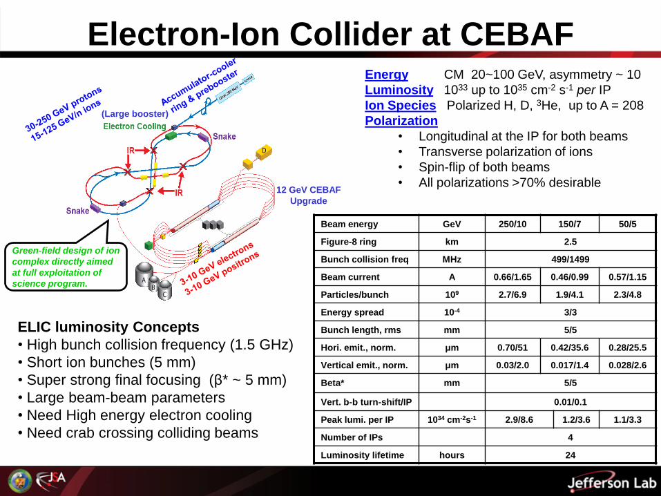
Electron-Ion Collider at CEBAF

12 GeV CEBAF

Upgrade

Green-field design of ion

complex directly aimed

at full exploitation of

science program.

(Large booster)

Beam energy GeV 250/10 150/7 50/5

Figure-8 ring km 2.5

Bunch collision freq MHz 499/1499

Beam current A 0.66/1.65 0.46/0.99 0.57/1.15

Particles/bunch 109 2.7/6.9 1.9/4.1 2.3/4.8

Energy spread 10-4 3/3

Bunch length, rms mm 5/5

Hori. emit., norm. μm 0.70/51 0.42/35.6 0.28/25.5

Vertical emit., norm. μm 0.03/2.0 0.017/1.4 0.028/2.6

Beta* mm 5/5

Vert. b-b turn-shift/IP 0.01/0.1

Peak lumi. per IP 1034 cm-2s-1 2.9/8.6 1.2/3.6 1.1/3.3

Number of IPs 4

Luminosity lifetime hours 24

Energy CM 20~100 GeV, asymmetry ~ 10

Luminosity 1033 up to 1035 cm-2 s-1 per IP

Ion Species Polarized H, D, 3He, up to A = 208

Polarization

• Longitudinal at the IP for both beams

• Transverse polarization of ions

• Spin-flip of both beams

• All polarizations >70% desirable

ELIC luminosity Concepts

• High bunch collision frequency (1.5 GHz)

• Short ion bunches (5 mm)

• Super strong final focusing (β* ~ 5 mm)

• Large beam-beam parameters

• Need High energy electron cooling

• Need crab crossing colliding beams

Introduction: Beam-Beam Physics

Transverse Beam-beam force

between colliding bunches • Highly nonlinear forces

• Produce transverse kick between colliding

bunches

Beam-beam effect• Can cause beam emittance growth, size

expansion and blowup

• Can induce coherent beam-beam instabilities

• Can decrease luminosity

linear part tune shift

nonlinear part tune spread & instability

Electron

bunch

Proto

n

bunch

IP

Electron bunchproton bunch

x

y

One slice from each

of opposite beams

Beam-beam force

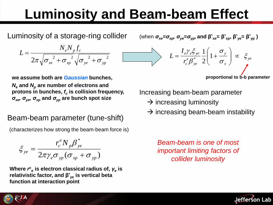
Luminosity and Beam-beam Effect

Luminosity of a storage-ring collider

22222 ypyexpxe

cpe fNNL

we assume both are Gaussian bunches,

Ne and Np are number of electrons and

protons in bunches, fc is collision frequency,

σxe, σye, σxp and σyp are bunch spot size

Beam-beam parameter (tune-shift)

(characterizes how strong the beam-beam force is)

)(2

*

ypxpype

yep

e

c

ye

Nr

Where rce is electron classical radius of, γe is

relativistic factor, and β*ye is vertical beta

function at interaction point

(when σxe=σxp, σye=σyp, and β*xe= β*

xp, β*ye= β*

yp )

proportional to b-b parameter

Increasing beam-beam parameter

increasing luminosity

increasing beam-beam instability

ye

x

y

ye

e

c

yeee

r

IL

1

2

1*

Beam-beam is one of most

important limiting factors of

collider luminosity

ELIC Beam-beam Problem

ELIC IP Design• Highly asymmetric beams (3-9GeV/1.85-2.5A and 30-225GeV/1A)

• Four interaction points and Figure-8 rings

• Strong final focusing (beta-star 5 mm)

• Very short bunch length (5 mm)

• Employs crab cavity

• Electron and proton beam vertical b-b parameters are 0.087 and 0.01

• Very large electron synchrotron tune (0.25) due to strong RF focusing

• Equal betatron phase advance (fractional part) between IPs

Short bunch length and small beta-star

• Longitudinal dynamics is important, can’t be treated as a pancake

• Hour glass effect, 25% luminosity loss

Large electron synchrotron tune

• Could help averaging effect in longitudinal motion

• Synchro-betatron resonance

Simulation Model, Method & Codes

Particle-in-Cell Method• Bunches modeled by macro-particles

• Transverse plane covered with a 2D mesh

• Solve Poisson equation over 2D mesh

• Calculate beam-beam force using EM fields on maeh points

• Advance macro-particles under b-b force

mesh point

(xi, yj)

BeamBeam3D Code

• Developed at LBL by Ji Qiang, etc. (PRST 02)

• Based on particle-in-cell method

• A strong-strong self-consistent code

• Includes longitudinal dim. (multi-slices)

Basic Idea of Simulations

Collision @ IP + transport @ ring

• Simulating particle-particle collisions by particle-in-cell method

• Tracking particle transport in rings

Code Benchmarking

• several codes including SLAC codes by

Y. Cai etc. & JLab codes by R. Li etc.

• Used for simulations of several lepton

and hardon colliders including KEKB,

RHIC, Tevatron and LHC

SciDAC Joint R&D program

• SciDAC grant COMPASS , a dozen

national labs, universities and companies

• JLab does beam-beam simulation for

ELIC. LBL provides code development,

enhancement and support

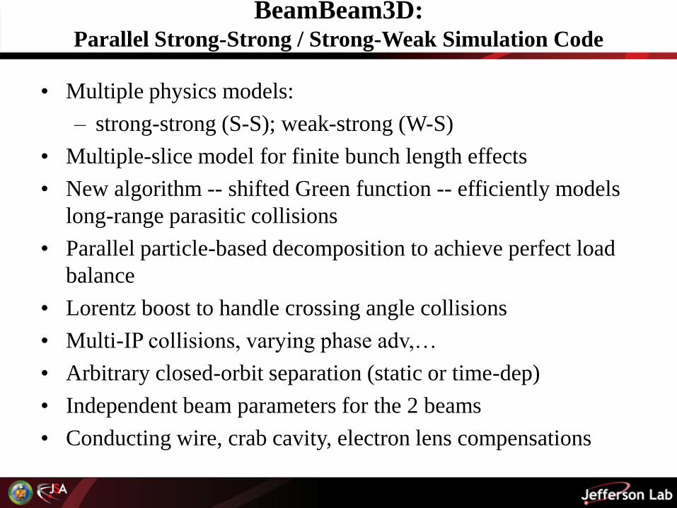
BeamBeam3D:Parallel Strong-Strong / Strong-Weak Simulation Code

• Multiple physics models:

– strong-strong (S-S); weak-strong (W-S)

• Multiple-slice model for finite bunch length effects

• New algorithm -- shifted Green function -- efficiently models

long-range parasitic collisions

• Parallel particle-based decomposition to achieve perfect load

balance

• Lorentz boost to handle crossing angle collisions

• Multi-IP collisions, varying phase adv,…

• Arbitrary closed-orbit separation (static or time-dep)

• Independent beam parameters for the 2 beams

• Conducting wire, crab cavity, electron lens compensations

Particle-In-Cell Method

Advance momenta

using radiation

damping and

quantum excitation

map

Advance momenta using beam-

beam forces

Field solution on grid to

find beam-beam forces

Charge deposition on

grid

Field interpolation at

particle positions

Setup for solving Poisson

equation

Initialize

particles

(optional)

diagnostics

Advance positions &

momenta using

external transfer map

21

20

21

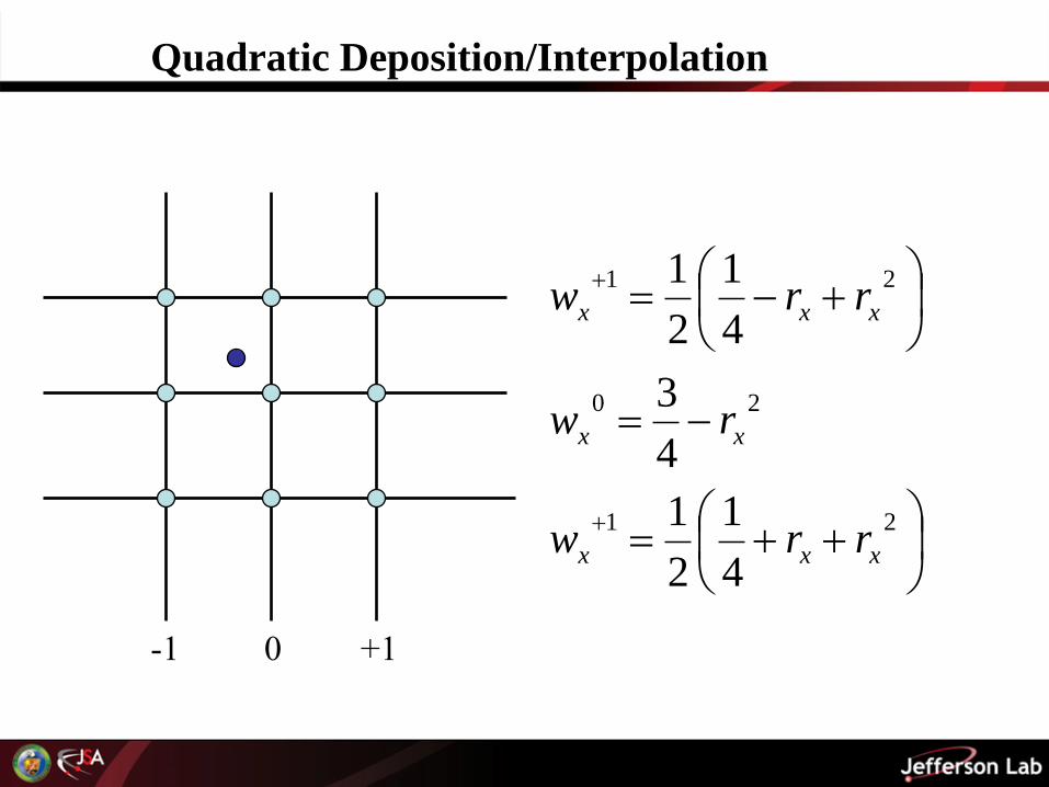
4

1

2

1

4

3

4

1

2

1

xxx

xx

xxx

rrw

rw

rrw

-1 0 +1

Quadratic Deposition/Interpolation

x

y

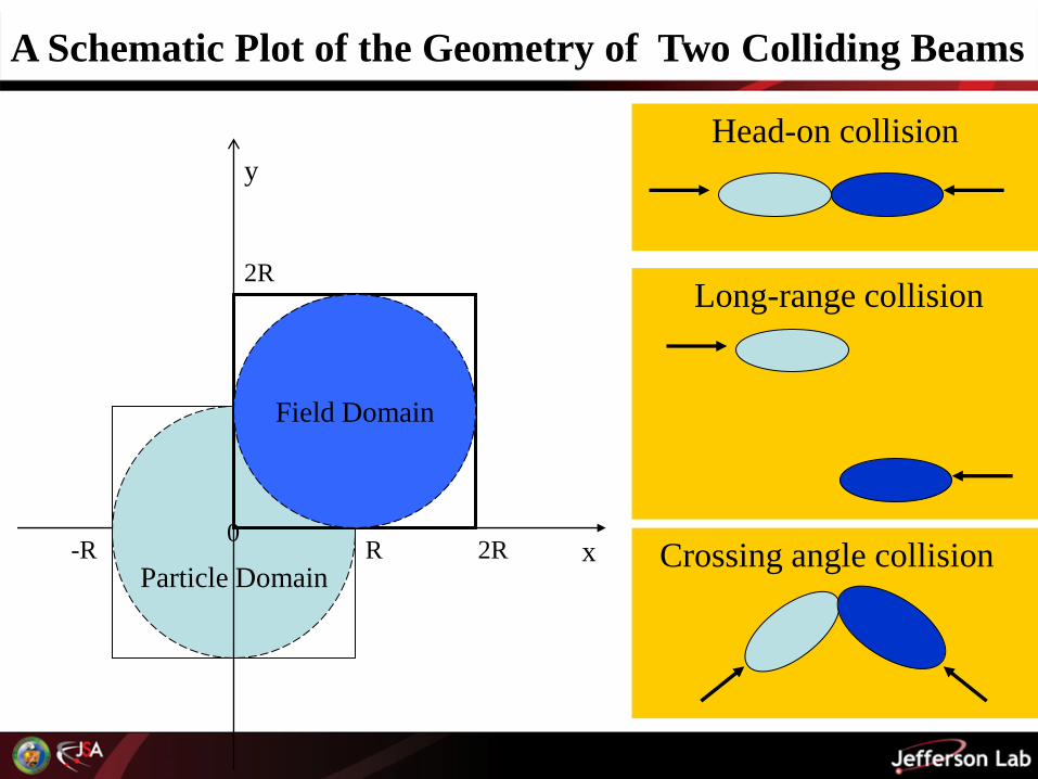
Particle Domain-R 2RR

2R

0

A Schematic Plot of the Geometry of Two Colliding Beams

Field Domain

Head-on collision

Long-range collision

Crossing angle collision

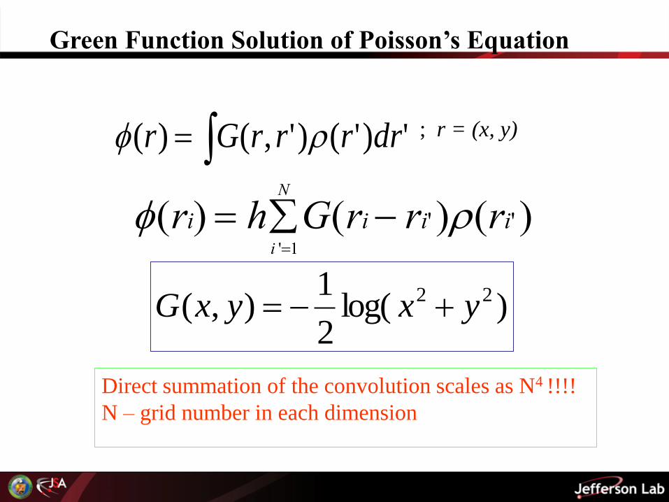
Green Function Solution of Poisson’s Equation

; r = (x, y) ')'()',()( drrrrGr

(ri) h G(rii '1

N

ri' )(ri' )

)log(2

1),( 22 yxyxG

Direct summation of the convolution scales as N4 !!!!

N – grid number in each dimension

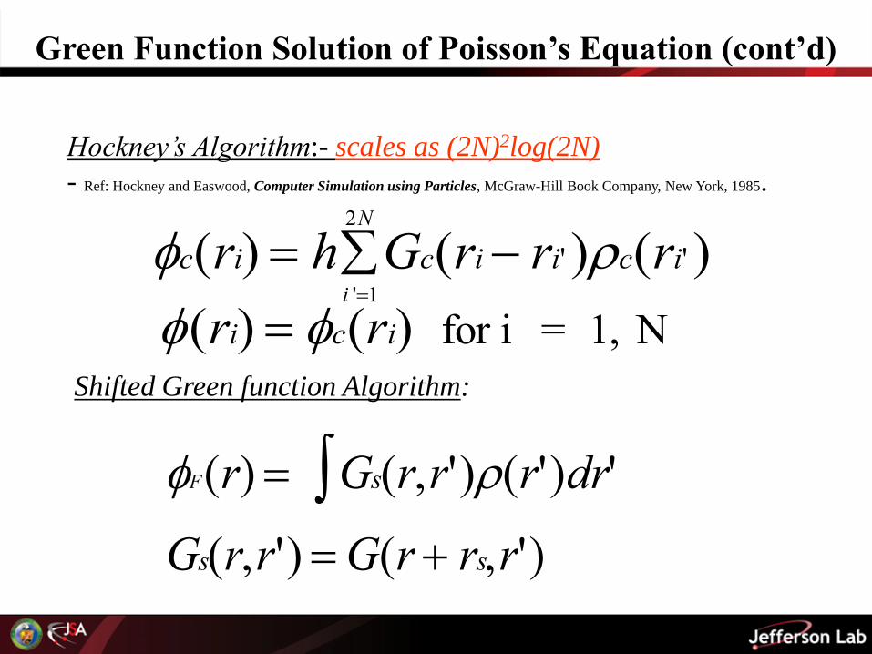
Green Function Solution of Poisson’s Equation (cont’d)

F(r) Gs(r,r')(r')dr'Gs(r,r') G(r rs,r')

c(ri) h Gc(rii '1

2N

ri' )c(ri' )

(ri) c(ri) for i = 1, N

Hockney’s Algorithm:- scales as (2N)2log(2N)

- Ref: Hockney and Easwood, Computer Simulation using Particles, McGraw-Hill Book Company, New York, 1985.

Shifted Green function Algorithm:

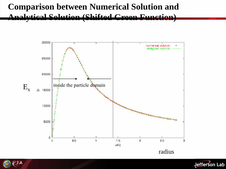
Comparison between Numerical Solution and

Analytical Solution (Shifted Green Function)

Ex

radius

inside the particle domain

Green Function Solution of Poisson’s Equation

(Integrated Green Function)

c(ri) Gi(rii '1

2N

ri' )c(ri' )

Gi(r,r') Gs(r,r')dr'

Integrated Green function Algorithm for large aspect ratio:

x (sigma)

Ey

B.Erdelyi and T.Sen, “Compensation of beam-beam effects in the Tevatron with wires,” (FNAL-TM-2268, 2004).

Model of Conducting Wire Compensation

(xp0,yp0)

test particle

*

,

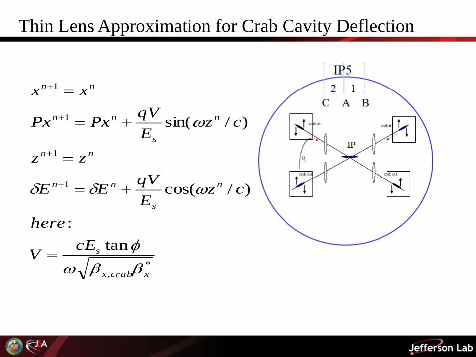
1

1

1

1

tan

:

)/cos(

)/sin(

xcrabx

s

nn

s

nn

nn

n

s

nn

nn

cEV

here

xczE

qVEE

zz

czE

qVPxPx

xx

Thin Lens Approximation for Crab Cavity Deflection

ELIC e-p Nominal Parameters

Simulation Model• Single or multiple IP, head-on collisions

• Ideal rings for electrons & protons

Using a linear one-turn map

Does not include nonlinear optics

• Include radiation damping & quantum excitations in the electron ring

Numerical Convergence Teststo reach reliable simulation results, we need

• Longitudinal slices >= 20

• Transverse mesh >= 64 x 128

• Macro-particles >= 200,000

Simulation Scope and Limitations• 10k ~ 30k turns for a typical simulation run

(multi-days of NERSC supercomputer)

• 0.15 s of storing time (12 damping times)

reveals short-time dynamics with accuracy

can’t predict long term (>min) dynamics

Proton Electron

Energy GeV 150 7

Current A 1 2.5

Particles 1010 1.04 0.42

Hori. Emit., norm. μm 1.06 90

Vert. Emit., norm. μm 0.042 3.6

βx / βy mm 5 / 5 5 / 5

σx / σy μm 5.7/1.1 5.7/1.1

Bunch length mm 5 5

Damping time turn --- 800

Beam-beam

parameter

0.002

0.01

0.017

0.086

Betatron tune

νx and νy

0.71

0.70

0.91

0.88

Synchrotron tune 0.06 0.25

Peak luminosity cm-2s-1 7.87 x 1034

Luminosity with

hour-glass effect

cm-2s-1 5.95 x 1034

Simulation Results: Nominal Parameters

0

0.1

0.2

0.3

0.4

0.5

0.6

0.7

0.8

0.9

1

0 1000 2000 3000 4000 5000

turns

l/l_

hg

lumi / lumi_0,hg

-0.2

0

0.2

0.4

0.6

0.8

1

1.2

0 1000 2000 3000 4000 5000

turns

<x>

an

d x

_rm

s (

no

rm)

<x>, e x_rms, e

<x>, p x_rms, p

-0.5

0

0.5

1

1.5

2

0 1000 2000 3000 4000 5000

turns

<y>

, y_rm

s (

no

rm

)

<y>, e y_rms, e

<y>, p y_rms, p

-0.2

0

0.2

0.4

0.6

0.8

1

1.2

0 1000 2000 3000 4000 5000

turns

<z>

, z_

rm

s

<x>, e z_rms, e

<z>, p z_rms, p

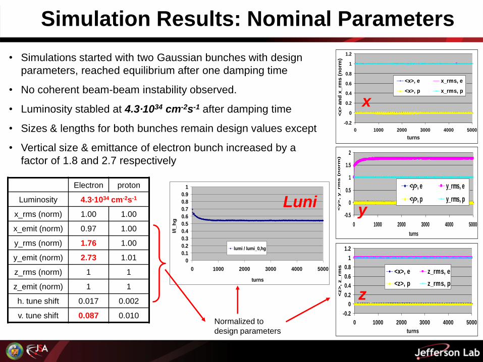
• Simulations started with two Gaussian bunches with design

parameters, reached equilibrium after one damping time

• No coherent beam-beam instability observed.

• Luminosity stabled at 4.3·1034 cm-2s-1 after damping time

• Sizes & lengths for both bunches remain design values except

• Vertical size & emittance of electron bunch increased by a

factor of 1.8 and 2.7 respectively

Electron proton

Luminosity 4.3·1034 cm-2s-1

x_rms (norm) 1.00 1.00

x_emit (norm) 0.97 1.00

y_rms (norm) 1.76 1.00

y_emit (norm) 2.73 1.01

z_rms (norm) 1 1

z_emit (norm) 1 1

h. tune shift 0.017 0.002

v. tune shift 0.087 0.010Normalized to

design parameters

x

y

z

Luni

Electron current dependence of Luminosity

• Increasing electron beam current by increasing bunch charge while bunch repetition rate remains the same, hence also increasing beam-beam interaction

• Luminosity increase as electron current almost linearly (up to 6.5 A)

• Proton bunch vertical size/emittance blowup when electron current is at above 7 A

• When electron beam reaches 5 A, proton dynamical vertical tune shift is 0.01 and above, while electron vertical tune shift goes down due to blowup of proton beam

• Coherent b-b instability observed at 7 ~ 7.5 A

0

0.02

0.04

0.06

0.08

0.1

2 3 4 5 6 7

electron current (A)

Verti

cal

Tu

ne s

hif

t

electron

proton

0

0.004

0.008

0.012

0.016

0.02

2 3 4 5 6 7

electron current (A)

Ho

riz

on

tal

Tu

ne S

hif

t

electron

proton

0

0.2

0.4

0.6

0.8

1

1.2

2 3 4 5 6 7electron current (A)

x_rm

s (

no

rm)

electron

proton

0.4

0.6

0.8

1

1.2

1.4

1.6

1.8

2

2 2.5 3 3.5 4 4.5 5 5.5 6 6.5 7 7.5

electron current (A)

Lu

mi

(no

rm)

Series1

Nominal

design

nonlinear/

coherent

0

0.2

0.4

0.6

0.8

1

1.2

1.4

1.6

1.8

2

2 4 6electron current (A)

y_rm

s (n

orm

)

electron

protonRapid growth

x

lumi

yξx

ξy

Coherent Beam-Beam Instability

1.4

1.42

1.44

1.46

1.48

1.5

0 5000 10000 15000 20000 25000 30000

turns

y_

rms

(n

orm

)

electron

proton

1.9

1.95

2

2.05

2.1

0 2500 5000 7500 10000 12500 15000

turns

lum

i (n

orm

)

luminosity

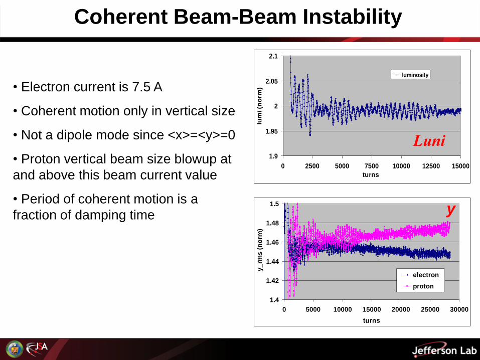
• Electron current is 7.5 A

• Coherent motion only in vertical size

• Not a dipole mode since <x>=<y>=0

• Proton vertical beam size blowup at

and above this beam current value

• Period of coherent motion is a

fraction of damping time

Luni

y

Proton current dependence of Luminosity

0

0.5

1

1.5

2

2.5

3

3.5

4

4.5

5

0.5 1.5 2.5 3.5

proton current (A)

y_rm

s (

no

rm)

electron

proton

0

0.2

0.4

0.6

0.8

1

1.2

0.5 1.5 2.5 3.5proton current (A)

x_rm

s (

no

rm)

electron

proton

0

0.05

0.1

0.15

0.2

0.25

0.3

0.35

0.5 1.5 2.5 3.5proton current (A)

Ve

rti

cal

Tu

ne s

hif

t electron

proton

0

0.01

0.02

0.03

0.04

0.05

0.06

0.07

0.5 1.5 2.5 3.5proton current (A)

Ho

rizo

nta

l T

un

e s

hif

t electron

proton

0.6

0.7

0.8

0.9

1

1.1

1.2

1.3

0.5 1.5 2.5 3.5proton current (A)

Lu

min

os

ity

(n

orm

)

Series1

Nominal design

nonlinear

• Increasing proton beam current by increasing proton bunch charge while bunch repetition rate remain same, hence also increasing beam-beam interaction

• Luminosity increase as proton beam current first approximately linearly (up to 1.5 A), then slow down as nonlinear beam-beam effect becomes important

• Electron beam vertical size/emittance increase rapidly

• Electron vertical and horizontal beam-beam tune shift increase as proton beam current linearly x

yξx

ξy

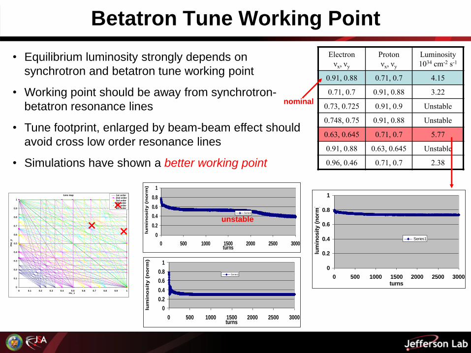
Betatron Tune Working Point

• Equilibrium luminosity strongly depends on

synchrotron and betatron tune working point

• Working point should be away from synchrotron-

betatron resonance lines

• Tune footprint, enlarged by beam-beam effect should

avoid cross low order resonance lines

• Simulations have shown a better working point

Electron

νx, νy

Proton

νx, νy

Luminosity

1034 cm-2 s-1

0.91, 0.88 0.71, 0.7 4.15

0.71, 0.7 0.91, 0.88 3.22

0.73, 0.725 0.91, 0.9 Unstable

0.748, 0.75 0.91, 0.88 Unstable

0.63, 0.645 0.71, 0.7 5.77

0.91, 0.88 0.63, 0.645 Unstable

0.96, 0.46 0.71, 0.7 2.38

0

0.2

0.4

0.6

0.8

1

0 500 1000 1500 2000 2500 3000turns

lum

ino

sit

y (

no

rm

)

Series1

nominal

tune map

0

0.1

0.2

0.3

0.4

0.5

0.6

0.7

0.8

0.9

1

0 0.1 0.2 0.3 0.4 0.5 0.6 0.7 0.8 0.9 1mu_x

mu

_y

1st order2nd order3rd order4th order5th order6th order

0

0.2

0.4

0.6

0.8

1

0 500 1000 1500 2000 2500 3000turns

lum

ino

sit

y (

no

rm

)

Series1

unstable

0

0.2

0.4

0.6

0.8

1

0 500 1000 1500 2000 2500 3000turns

lum

ino

sit

y (

no

rm)

Series1

New Working Point (cont.)

0.5

1

1.5

2

2.5

2 3 4 5 6 7 8

electron current (A)

lum

i (no

rm)

Old Working Point

New Working Point

1

1.2

1.4

1.6

1.8

2 3 4 5 6 7 8

electron current (A)

y_rm

s (n

orm

)

electron, old WP proton, old WP

electron, new WP proton, new WP

0.4

0.6

0.8

1

1.2

1.4

1.6

1.8

1 1.5 2 2.5 3 3.5 4

proton current (A)

lum

i (n

orm

)

old Working Point

New Working Point

1

1.5

2

2.5

3

3.5

4

4.5

5

2 2.5 3 3.5 4

proton current (A)y

_rm

s (

no

rm)

Old WP, electronOld WP, protonNew WP, electronNew WP, proton

Simulation studies show

• systematic better luminosity over beam current regions with new working point,

• coherent instability is excited at same electron beam current, ~ 7 A

Multiple IPs and Multiple Bunches

ELIC full capacity operation

• 4 interaction points, 1.5 GHz collision frequency

• 20 cm bunch spacing, over 10500 bunches stored for each beams

• Theoretically, these bunches are coupled together by collisions at 4 IPs

• Bunches may be coupled through other beam physics phenomena

• A significant challenges for simulation studies

What concerns us• Multiple bunch coupling

• Multiple IP effect

• Introducing new instability and effect on working point

• Earlier inciting of coherent beam-beam instability

• New periodicity and new coherent instability (eg. Pacman effect)

Reduction of Coupled Bunch Set

1

2

34

5

6

7

8

910

11

12

13

14

1516

17

18

19

20

2122

23

24

1

2

34

5

6

7

89 10

11

12

13

14

15 1617

18

19

202122

23

24

~Dip-ip

Dip-ip

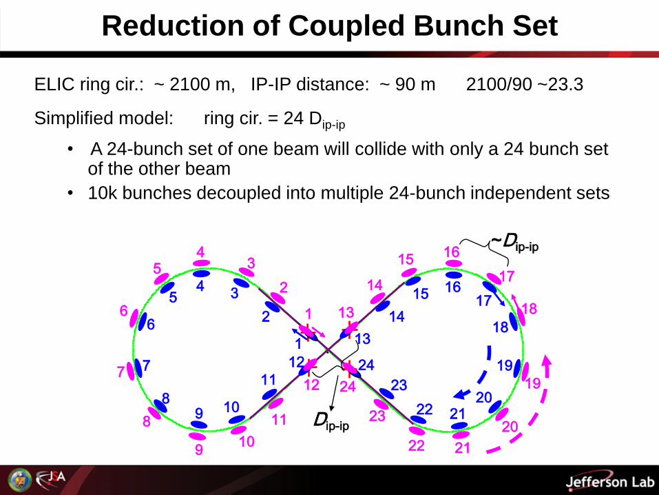
ELIC ring cir.: ~ 2100 m, IP-IP distance: ~ 90 m 2100/90 ~23.3

Simplified model: ring cir. = 24 Dip-ip

• A 24-bunch set of one beam will collide with only a 24 bunch set of the other beam

• 10k bunches decoupled into multiple 24-bunch independent sets

step 1 2 3 4 5 6 7 8 9 10 11 12 13 14 15 16 17 18 19 20 21 22 23 24

IP1 1

1

24

2

23

3

22

4

21

5

20

6

19

7

18

8

17

9

16

10

15

11

14

12

13

13

12

14

11

15

10

16

9

17

8

18

7

19

6

20

5

21

4

22

3

23

2

24

IP2 2

2

1

3

24

4

23

5

22

6

21

7

20

8

19

9

18

10

17

11

16

12

15

13

14

14

13

15

12

16

11

17

10

18

9

19

8

20

7

21

6

22

5

23

4

24

3

1

IP3 13

13

12

14

11

15

10

16

9

17

8

18

7

19

6

20

5

21

4

22

3

23

2

24

1

1

24

2

23

3

22

4

21

5

20

6

19

7

18

8

17

9

16

10

15

11

14

12

IP4 14

14

13

15

12

16

11

17

10

18

9

19

8

20

7

21

6

22

5

23

4

24

3 1 2

2

1

3

24

4

23

5

22

6

21

7

20

8

19

9

18

10

17

11

16

12

15

13

Multiple IPs and Multiple Bunches

Collision Table

• Even and odd number bunches also

decoupled

• When only one IP, one e bunch

always collides one p bunch

• When two IPs opens on separate

crossing straights and in symmetric

positions, still one e bunch collides

with one p bunch

Full scale ELIC simulation model

• 12 bunches for each beam

• Collisions in all 4 IPs

• Bunch takes 24 steps for one

complete turn in Figure-8 rings

• Total 48 collisions per turn for

two 12-bunch sets

Multiple IPs and Multiple Bunches (cont.)

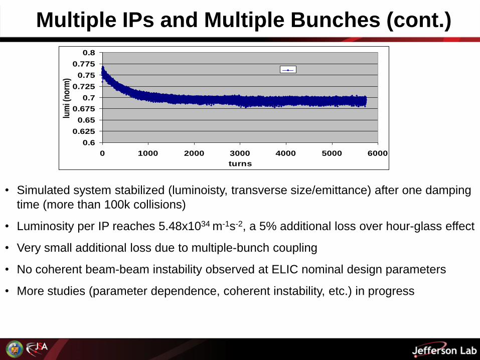
• Simulated system stabilized (luminoisty, transverse size/emittance) after one damping

time (more than 100k collisions)

• Luminosity per IP reaches 5.48x1034 m-1s-2, a 5% additional loss over hour-glass effect

• Very small additional loss due to multiple-bunch coupling

• No coherent beam-beam instability observed at ELIC nominal design parameters

• More studies (parameter dependence, coherent instability, etc.) in progress

0.6

0.625

0.65

0.675

0.7

0.725

0.75

0.775

0.8

0 1000 2000 3000 4000 5000 6000

turns

lum

i (n

orm

)

Summary

• Beam-beam simulations were performed for ELIC ring-ring design with nominal parameters, single and multiple IP, head-on collision and ideal transport in Figure-8 ring

• Simulation results indicated stable operation of ELIC over simulated time scale (10k ~ 25k turns), with equilibrium luminosity of 4.3·1034 cm-2s-1,roughly 25% reduction for each of hour-glass and beam-beam effects

• Studies of dependence of luminosity on electron & proton beam currents showed that the ELIC design parameters are safely away from beam-beam coherent instability

• Search over betatron tune map revealed a better working point at which the beam-beam loss of luminosity is less than 4%, hence an equilibrium luminosity of 5.8·1034 cm-2s-1

• Multiple IP and multiple bunch simulations have not shown any new coherent instability. The luminosity per IP suffers only small decay over single IP operation

Outlook

• Toward more realistic model of beam transport

Needs of including real lattice and magnet imperfections

Trade-off (due to computing power limit): full particle-tracking in ring and

weak-strong beam model

Short term accurate vs. long term (inaccurate) behavior

• Move to space charge dominated low ion energy domain

pancake approximation of beam-beam force vs. full 3D mash calculation

New limit = Laslett tune-shift + beam-beam tune-shift ?

• Advanced interaction region design

Crab crossing

Traveling focusing

Crab waist

Future Plan

• Continuation of code validation and benchmarking

• Single IP and head-on collision

– Coherent beam-beam instability

– Synchrot-betatron resonance and working point

– Including non-linear optics and corrections

• Multiple IPs and multiple bunches

– Coherent beam-beam instability

• Collisions with crossing angle and crab cavity

• Beam-beam with other collective effects

• Part of SciDAC COMPASS project

• Working with LBL and TechX and other partners for developing and

studying beam dynamics and electron cooling for ELIC conceptual

design

Acknowledgement

• Helpful discussions with R. Li, G. Krafft, Ya. Derbenev of

JLab

• JLab ELIC design team

• Support from DOE SciDAC Grant

• NERSC Supercomputer times