Page 1
City University of New York (CUNY) City University of New York (CUNY)
CUNY Academic Works CUNY Academic Works
Dissertations and Theses City College of New York
2013
Application of Computational Fluid Dynamics as a Simulation-Application of Computational Fluid Dynamics as a Simulation-
based Design Guide in a Microfluidic 3D Living Cell Array (3D LCA) based Design Guide in a Microfluidic 3D Living Cell Array (3D LCA)
Device Device
A.H. Rezwanuddin Ahmed CUNY City College
How does access to this work benefit you? Let us know!
More information about this work at: https://academicworks.cuny.edu/cc_etds_theses/176
Discover additional works at: https://academicworks.cuny.edu
This work is made publicly available by the City University of New York (CUNY). Contact: [email protected]
Page 2
Application of Computational Fluid Dynamics as a Simulation-based Design Guide in a
Microfluidic 3D Living Cell Array (3D LCA) Device
Thesis
Submitted in partial fulfillment of
the requirement for the degree
Master of Engineering (Biomedical)
at
The City College of New York
of the
City University of New York
by
A.H. Rezwanuddin Ahmed
August 2013
Approved:
________________________________
Professor Sihong Wang, Thesis Advisor
_________________________________
Professor Mitchell Schaffler, Chairman
Department of Biomedical Engineering
Page 3
Abstract
The use of computational fluid dynamics (CFD) as a tool in the aerodynamics and oil
industry provides a reinforcement to efficiency in the design of aircrafts or for understanding the
flow through pipes. A similar approach can be taken towards microfluidics, where traditionally
devices have been designed based on experience or physiological replication, and a CFD
simulation is shown post-manufacture to show the flow and diffusion patterns present. In this
study, a reverse approach is suggested, by designing the device first in CFD and perform
simulations on variations of alterable parameters to get insight on how the changing parameters
affect the conditions within the device. A 3D Microfluidic Living Cell Array (3D LCA) wherein
cells are embedded in a hydrogel is used as the model to perform the simulations on. It is shown
that alterations of certain parameters (such as pore size) can have drastic effects on the nutrient
supply and waste removal mechanics of the 3D cell microchamber, while other factors such as
the permeability of the medium of cell culture (hydrogel) does not affect the glucose
concentration but does affect the O2 and CO2 concentrations generated within the microchamber.
Page 4
Acknowledgements
The amount of work, time and dedication put into this thesis would not be possible without the full
support, advise, and mentorship of my advisor, Dr. Sihong Wang, to whom I owe my sincerest gratitude. I
am also very grateful to have the privilege of presenting to the distinguished professors who are part of
the committee, including Dr. Tarbell, Dr. Vazquez, Dr. Fu, and Dr. Wang.
My heartfelt thanks goes to my best friend and mentor, Dr. Zeynep Dereli, who has tried her best to reach
out when I needed guidance or assistance.
To my family, who cannot be here for my defense, but always keep me in their minds and their hearts, I
have more than just a heartfelt gratitude for all the years of support and camaraderie.
And lastly, to all my companions in the lab and at City College who have offered help in their own way
by friendship or use of their resources - Dr. Chenghai Li, Joanne Lee, Kristifor Sunderic, Dionne Dawkins,
Paolo Palacio, Yury Borisov, Liudi Yang, and Gary Ye, you have my gratitude.
Page 5
Table of Contents
1. Introduction ....................................................................................................................................... 1
Dynamic Macro-systems .............................................................................................................. 1
The tumor microenvironment ....................................................................................................... 2
Developing a 3D Microfluidic Living Cell Array (3D LCA) Device ........................................... 3
The importance of design ............................................................................................................. 4
2. Methods and Materials ...................................................................................................................... 5
Equations and Assumptions of Importance to Fluids Mechanics Models in Biological Systems 5
Preliminary Mass, Momentum, and Energy Conservation Equations .......................................... 6
Flow Through Porous Media ........................................................................................................ 8
Diffusivity and Convection ........................................................................................................... 9
Reaction Mechanisms and Rates .................................................................................................. 11
Parameters defined in or by the model ......................................................................................... 13
Peclet Number ............................................................................................ 14
Diffusivities used ........................................................................................ 14
Input Concentrations................................................................................... 15
Reaction Rate .............................................................................................. 15
Chamber parameters used ........................................................................... 16
The Model: Ansys Fluent v14
3. Results and Discussion:
Measurement of Glucose Consumption Rate ............................................................................... 19
Calculating Cell Consumption Rate to use in the Model .............................................................. 21
Representation of Data/Results ..................................................................................................... 22
Changes in Pore Size .................................................................................................................... 24
Changes in Membrane Thickness ................................................................................................. 31
Changes in Permeability ............................................................................................................... 39
The unexpected Case 44
4. Conclusion ................... .................................................................................................................... 51
5. Summary ...................... .................................................................................................................... 53
6. References .................... .................................................................................................................... 54
7. Supplemental Figures ... .................................................................................................................... 56
Page 6
1 | P a g e
1. Introduction
Computational Fluid Dynamics (CFD) has taken tremendous strides since its advent in the earlier
half of the twentieth century. Although the principles were there, the execution of those theories were
restrained until the computer industry, driven partly (but strongly) by the necessity of computing power to
solve computational fluid dynamics problems, took great leaps in producing more powerful processors
and efficient algorithms since the 1970's[1]. The field of CFD has come far enough such that the
ownership of CFD software is congruent to owning a wind virtual tunnel. Although computational
techniques will never replace true experimental manifestations - since mathematical equations are only
models of what we perceive and not a holistic representation of every component a system contains -
most of the equations used in the field are derived from physically or experimentally accurate and
observed principles. Amongst these principles are the Navier-Stokes' equations, the diffusion (or heat)
equation, Stokes-Einstein equation (which represents the diffusivity of molecules based on their size and
affinity), the Darcy and Brinkman equations that define porous flow, and many more. Simultaneous
solutions of these equations via numerical approximation are what gives CFD its convenience and power.
Dynamic Macro-Systems
The design of dynamic flow systems already exist in the form of various larger devices and in
microfluidic devices. Amongst the larger devices are systems that perform on a scale that would not be
feasible on a simple microscopic scale - such as bioreactors seeded with hepatocytes, renal dialysis
systems, or even artificial hearts. In the case of a bioreactor, the supply of nutrients to the hepatocytes and
the corresponding removal of wastes from the bioreactor is of quintessential importance to keep the cells
in the natural state (and healthy) for as long as possible. [2] In devices such as the artificial heart, the
diffusion factors of nutrients are not pertinent, rather, the flow pattern within the device such as to provide
the body with a proper blood supply ( approx. 4-5 L/min) and to prevent the damage of the device (such
as from cavitation) is to be ensured. Thus, the dynamic demands of various devices may vary from simple
flow requirements to the maintenance of a complex balance of nutrient supply and demand.
Page 7
2 | P a g e
Devices could be designed based on experience or physiologically relevance. One example is to
design a bioreactor (or microfluidic device) in which the distance between the perfusing media and the
hepatocytes (or cultured cells) are no more than 100-200 µm away from the perfusing channel. This
distance comes from Warburg's calculations for the diffusion limitation of a small molecule (such as
oxygen or glucose), and has been experimentally or physiologically confirmed by others.[3]
The Tumor Microenvironment
The tumor microenvironment is comprised of tumor cells (parenchymal cells) and the associated
stromal structure and cells, including carcinoma-associated fibroblasts, leukocytes, bone-marrow derived
cells, and blood and lymphatic vascular endothelial cells. The microenvironment is also characterized by
irregular vasculature, high interstitial fluid pressure, high pH levels, abnormal inflammatory response and
metabolic chaos.[4-7] Although it is argued as to whether this chaotic environment is the cause or effect
of the tumor microenvironment, it is certain that the carcinogenic disposition of cells and such an aberrant
microenvironment are correlated.[8] The chaotic microenvironment can promote tumor progression, as
various studies have shown.[9-11] These studies also suggest that the normalization (return to normal
function) of blood vessels by rendering them less leaky through administration of chemicals that reduce
vascular permeability (e.g. VEGF inhibitors) can improve the prognosis of the patient and work
synergistically with chemo- or radio-therapy.[4, 6, 7] One of the hallmarks of the tumor
microenvironment is hypoxia, which in turn promotes the accumulation of the constitutively produced
hypoxia-inducing factor-α (HIF-α), further stimulating tumor progression by promoting various other
inducible factors in the cells.[10, 12, 13] Some of the inducible enzymes or factors by HIF-α include
vasoactive proteins (endothelin-1, NO synthase-2, plasminogen activator inhibitor-1, vascular endothelial
growth factor(VEGF), VEGF receptor), hormones and receptors (such as α1B-adrenergic receptors,
transforming growth factor β5), and enzymes that promote energy and iron metabolism. All these factors
help the cell to adapt to the low-oxygen environment.[14]
Page 8
3 | P a g e
Developing a 3D microfluidic living cell array (3D LCA) device
One of the goals in trying to design a microfluidic device is to mimic the tumor
microenvironment, including the blood vessel which supplies the nutrients and a scaffold (gel) into which
the perfusing nutrients can diffuse into while housing the cells. Designing a device for investigating
physiologically accurate cellular activity will by necessity be a 3D culture with a continuous perfusion,
as opposed to simple, static 2D (or 3D) culture. Static 2D/3D cultures or animal models are poor (or
inaccurate) imitations of the true in vivo dynamic representation of human physiological conditions.
Mimicking the in vivo conditions by 3D in vitro dynamic models will provide a more accurate drug
responses of cancer cells (cell lines or biopsy samples).A 3D microfluidic LCA mimicking such
microenvironment enables accurate, high-throughput drug screening on an efficient scale. Previous work
from our lab produced a device consisting of multiple wells arranged in an array format witheach well
being an individual cell culture chamber.[15] There are three layers in the device:(1) the top rectangular
channels with a width of 790 µm (corresponding to the width of pulmonary veins, >500 µm) and height
of 130 µm; (2) a middle and gas permeable membrane with 40 µm clustered pores, which provides a
frame over which endothelial cells can be cultured and still allow perfusion and diffusion between the top
channel and the bottom chamber; and (3) the bottom chambers right underneath the clusteredd pores with
a diameter of 770 µm, and a depth of approximately 100 µm, wherecells can be are seeded and
encapsulated inhydrogel (e.g. PuraMatrix). The measured viscous resistance
of PuraMatrix
is 5x10¹⁴
m-2
, which is a first step in emulating the stiffness of the tumor microenvironment In the tumor
microenvironment, depending on the tumor site, the permeability can increase by up to two orders of
magnitude (to the order of 5x10¹²
m-2
visc. resistance)[16]. The lack of functional lymphatic systems
within a solid tumor is captured in the device by not having an outlet at the bottom of the chamber.
The importance of design
Page 9
4 | P a g e
Designing by experiment does not always meet the conditions we need to mimic in a cell culture
model Instead of taking a trial-and-error approach by intuition, or using a post-manufacture CFD analysis
to “show” what is going on in the device, it would be more economical and efficient to use CFD to guide
the understanding of how different device parameters would provide a different set of conditions in the
cell culture. The current 3D LCA device is hardly a perfect representation of the tumor microenvironment,
but is a step towards that goal.A CFD model can provide an insight into the effects on flow and diffusive
profiles induced by changing the porosity and thickness of simulated basement membrane (the middle
layer) or by changing the permeability of the microenvironment (the hydrogel). By understanding the
physiological effects that are being recreated ,such as low pO2 and pH, or high interstitial fluid pressure, it
is possible to grasp the scope of the environment that the seeded tumor cells in the device are exposed to,
and how these parameters can be changed to provide a device with the optimal (or desired) conditions.
For instance, if the pleiotropic effects of hypoxia needs to be studied (such as testing drugs that only work
in hypoxic conditions [8], there would be a necessity to induce a relatively hypoxic state in the
extracellular environment.
The computational power of CFD is avidly used in the aerodynamics and oil industry to simulate
models of flow over vehicles or of oil flow in pipes prior to the construction of the actual objects[1]. A
similar approach can be taken towards the design of biological devices such as 3D microfluidic devices.
In this study, only one well of the entire device is considered to keep the computational time and
resources within reason. By altering certain physical parameters of the device itself, and by providing the
correct inputs to the system, a generalized model is obtained which provides the optimal conditions that
are sought from the device to be built. Although there will be practical limitations of the accuracy of the
device itself (for instance, the actual permeability of the constructed hydrogel in the device may not be
fully isotropic and slightly different from the parameter input into the software) as well as manufacturing
errors that cannot be pre-determined, the simulated scenarios of the environment produced in the device
itself will provide a starting point on the selections to use that will optimize the parameters (e.g. fluid flow
Page 10
5 | P a g e
through the device, pO2 and pH in the cell culture chamber, etc.) by showing effects on such parameters
that are induced from alterable parameters in the device simulation (e.g. pore size of the membrane within
the device, permeability of the hydrogel, concentration of glucose or other nutrients, etc). The discrepancy
of the simulation from the actual observed result can be noted later, after the device has been
manufactured and experimental tests are run.
2. Methods & Materials
Equations and Assumptions of Importance to Fluid Mechanics Models in Biological Systems
Computational Fluid Dynamics obeys the principles of fluid dynamics, which are derived from
observed physical principles. The equations that are most important and used in the computation are
provided in this section. These concepts are inherently included in the software package used, ANSYS
Fluent, part of the ANSYS®v14 Workbench. ANSYS Fluent is a powerful CFD tool with customizable
geometries, material properties, flow profiles, and reaction rates, which are all essential to the definition
of the model being simulated. It is important to understand the equations that are being implemented or
worked with as a mathematical model with incorrectly formalized parameters will provide an incorrect
and most likely irrelevant solution that may evade verification due to the lack of realistic experimental
implementation.
Preliminary Mass, Momentum, and Energy conservation Equations
Non-uniform flow patterns can lead to poor nutrient supply and non uniform shear stress
distribution. Although in this paper the focus is not placed on shear stresses, it may be pertinent to those
who wish to culture cells that are sensitive to shear stresses (such as endothelial cells). Typically in a µ-
fluidic (microfluidic) device, the flow profiles are well defined if the parameters are chosen accordingly.
The continuity equation which essentially comes from the reasoning that mass can neither be
gained nor lost but only transferred, is represented as:
Page 11
6 | P a g e
(1a) or
(1b)
Where V is the velocity vector of the fluid flow, is the fluid density,
is the total differential change in
,
is the partial change of density with respect to time (local change), and is the del operator as
defined in standard vector calculus books.
The momentum conservation (Navier-Stokes) equations are as follows:
(2a)
(2b)
(2c),
Where is the fluid pressure, is the fluid density, u, v, and w are the velocity components in the
Cartesian x,y, and z directions, are elements from the shear stress matrix in the respective direction
(i)along the plane defined by the jth normal vector, and is the body force per unit volume in the i
th
direction.
The Navier-Stokes’ Equations for viscous Newtonian fluids is given by the set of equations in
2a-2c, with the added constitutive information for the stress-viscosity relationship ( is proportional to
velocity gradients):
, (3a)
, (3b)
,(3c)
, (3d)
, (3e)
. (3f)
Where is the second viscosity coefficient, while is the molecular viscosity. As per Stokes's hypothesis,
Page 12
7 | P a g e
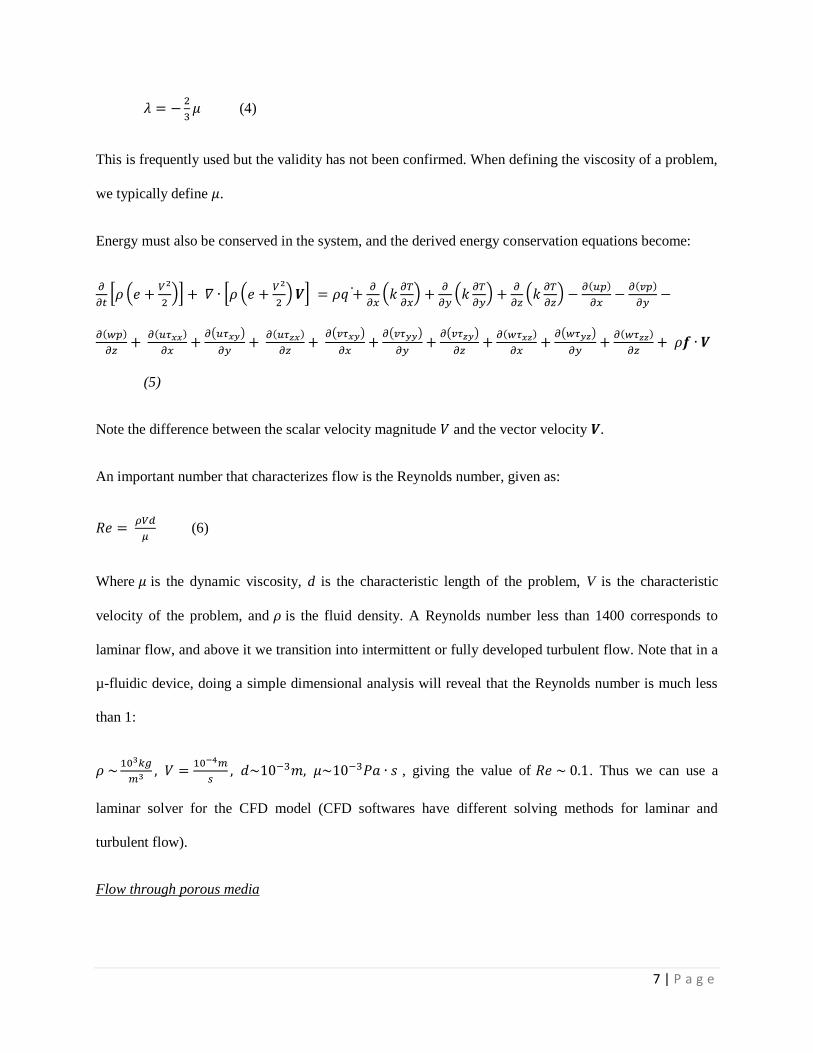
(4)
This is frequently used but the validity has not been confirmed. When defining the viscosity of a problem,
we typically define .
Energy must also be conserved in the system, and the derived energy conservation equations become:
(5)
Note the difference between the scalar velocity magnitude and the vector velocity .
An important number that characterizes flow is the Reynolds number, given as:
(6)
Where is the dynamic viscosity, d is the characteristic length of the problem, V is the characteristic
velocity of the problem, and is the fluid density. A Reynolds number less than 1400 corresponds to
laminar flow, and above it we transition into intermittent or fully developed turbulent flow. Note that in a
µ-fluidic device, doing a simple dimensional analysis will reveal that the Reynolds number is much less
than 1:
, giving the value of . Thus we can use a
laminar solver for the CFD model (CFD softwares have different solving methods for laminar and
turbulent flow).
Flow through porous media
Page 13
8 | P a g e
Newtonian fluid flow through a porous medium at low Reynolds number could be modeled using Darcy’s
flow, given as:
(7a),
(7b),
where 'q' is the fluid velocity (calculated), n is the porosity, and vs is the true fluid velocity to account for
the limited volume introduced by having a porous material.
The scale of µ-fluidic devices are so small that the Reynolds number is small (<1) by the very
implementation of the device. However, Darcy’s flow does not capture the viscous effects, and inviscid
flow typically cannot account for the no-slip boundary conditions. For modeling flow through thin slices
or small sections, the gradient of velocity becomes an important factor and cannot be neglected by using
simply Darcy’s flow model. In such a case, the Brinkman model is used, which accounts for the viscous
effects of the fluid. The equation is given as:
(8)
Where is the superficial velocity vector, is the viscosity, and the permeability of the porous
medium.
Note that the equation reduces to the Navier-Stokes equation or Darcy’s equation depending on
whether the viscous forces or drag forces become dominant. Thus, in the transition between these two
flows – such as flow in the µ-fluidic device where the flow goes from free-flow into a porous media, the
full Brinkman implementation should be used. This allows the continuity of velocity and shear stresses,
especially at the interface. Note as an example that flow in open channels (permeability being almost
infinite) will reduce the Brinkman equation to the Navier-Stokes equation for incompressible flow. [17]
Diffusivity and Convection
Page 14
9 | P a g e
The primary purpose to having a constant flow is to mimic, to a certain degree, the physiological
condition of having a continuous supply of fresh nutrients as well as a continuous “exhaust” or flushing
out of waste products. A well balanced system should match the supply of nutrients to the reaction rate of
the cells such that there is neither an accumulation nor a deficit. Thus, in a well balanced system, at
dynamic equilibrium, the local increase in concentration
should be 0. The convection-diffusion
equation is as follows:
, (9a)
(9b)
Where the variables are:
C: concentration of the species (mol/m3),
N: molar flux (mol/m2.s),
R: consumption rate of the species (mol/m3.s)
v: velocity as calculated from Brinkman’s equation (m/s), and
D: diffusivity of the solute (m2/s)
At equilibrium,
= 0, reducing the equation to:
(9c)
Bulk diffusivity varies from the actual effective diffusivity since the entire area normal to the
diffusive flux is not available in the porous medium. The effective diffusivity of a species through a
porous structure thus differs from the bulk diffusivity due to the porosity and tortuosity of the material.
Tortuosity is defined as the ratio between the actual distance traveled by a species particle between two
Page 15
10 | P a g e
points and the smallest distance between those very two points, and it is commonly represented by the
variable τ, and this often takes values ranging from 2 to 10.[18]Representing the porosity as , there is an
equation that relates the bulk diffusivity to diffusivity throughout a porous medium (using oxygen as an
example):
, (10)
Where is the bulk diffusivity of the species (in this case oxygen) in the media perfusing through the
porous structure, and τ are, as aforementioned, the porosity and tortuosity, respectively.
A system may or may not be diffusion limited, and the quantitative way to acknowledge this is to
calculate the Peclet (Pe) number. The Pe number is a ratio of the convective transport and the dispersion
(or diffusive) coefficient, and is given as:
(11)
Where D is the diffusion coefficient as before, is the characteristic fluid velocity, and d is the
characteristic length of the model in use. A Pe number between 0 and 1 indicates that the transport of the
species to the site of interest is primarily diffusion limited, at larger Pe the transport of the species is
mainly convection-driven.
A model equation by Warburg predicts the possible thickness of a region of healthy cells possible
by diffusion alone using blood as the non-circulating fluid would be 1mm for a cylinder-shaped tissue or
complete developing organism, calculated by:
(12)
Where is the maximum distance, is the bulk diffusivity of oxygen in blood, is the partial
pressure in the culture medium (or blood), and is the rate of oxygen consumption in the tissue. In
Page 16
11 | P a g e
physiological conditions, especially around capillaries, the distance limit set by diffusive transport of
nutrients is typically 100-200 µm, cells beyond this region enter a state of hypoxia (such as the necrotic
cells in the center of a solid tumor mass deprived of oxygen due to their distance from active capillaries at
the tumor periphery). This phenomenon is also commonly noticed in bioreactor design, where, for a
hepatocyte culture, is was shown that a reactor design that relies solely on diffusion for mass transfer
requires that the cells be within 150-200 µm of an oxygen source to survive and proliferate.
Reaction Mechanisms and Rates:
Reaction kinetics can be implemented by user-defined methods into a CFD application. The bulk
volumetric reaction can be defined that occurs at given regions or zones in a model (such as the bottom
chamber, the top channel, or the middle membrane) – or can be discretized based on location within the
model. It lies upon the user to select the model most suitable for the reaction model.
Reactions that define the glucose consumption or oxygen consumption rate are typically modeled
using Michaelis-Menten kinetics:
(13)
Where is the reaction rate (positive indicates creation of the species), is the maximum reaction rate
possible (such as by increasing the species), is the Michaelis constant (the concentration of the species
at which the reaction rate is half of ), and is the current concentration of the species itself.
In a culture where there is cell growth, the reaction rate is modeled as:
(14)
Where is the cell concentration, and is the yield coefficient of cell concentration on component
concentration (how the growth rate affects the consumption of the species), and is the maintainence
Page 17
12 | P a g e
rate for the cells are currently in existence. Under limiting nutrient and space considerations (and cell-cell
contact inhibition), the growth of cells can typically be modeled as:
(15)
where is the growth rate constant, and is the maximum cell density permissible. The nutrient
limitation is inherently considered in the growth rate by modeling it as another equation:
(16)
Where is the concentration of the nutrient as in the Michaelis-Menten equation.
The typical values for the consumption rate used in a 3D model are derived from 2D cultures
done on a plastic culture surface. Cells respond differently when cultured on different substrates or when
grown in different configurations (2D or 3D), and experimentally determined kinetic parameters that are
truer to 3D culture should be collected in order to make the CFD model closer to a realistic realization.
However, for the purposes of this paper, the cultures were done in a 2D culture plate using PC9
non-small-cell lung cancer cells. The procedure and data are discussed later, in the “Parameters defined in
the model” sub-section and the Results section.
Consider the quasi-static case in which the residence time of the nutrients is much smaller than
the cell growth rate, in which case we can ignore the cell growth rate and model the system at a fixed,
known, cell density. In this case, eqn. 14 reduces to . An important assumption here is that is
much smaller than , since otherwise if >> , the term becomes large enough such that the
term
cannot be ignored. A small value also denotes that the nutrient uptake rate is almost independent in
sensitivity to the local concentration of the nutrient itself. Such examples are seen in chondrocytes and
hepatocytes where the uptake rate is reduced by only 2-10% with a 50% reduction in oxygen
Page 18
13 | P a g e
concentration. On the other hand, there was a 35% reduction in smooth muscle cells for the same 50%
reduction in oxygen tension.[17]
Parameters defined in or by the model
The shear stress in a rectangular channel is given as:
,
where Q is the flow rate, w and h are the channel width and height respectively, and µ is the
dynamic viscosity of the fluid in question. Using a flow rate of 100 µm/sec, the calculated shear stress
value is = 0.05dyne/cm2, which is within the ideal range for a wide variety of mammalian cell lines. (<0.1
dyne/cm2 and >0.01 dyne/cm
2)[3]As described before, the simulated device comprises of one well in the
device, which is made up of three layers: (1) a top layer with a width of 790 µm, a height of 100 µm, and
a length of 1600 µm, (2) a gas-permeable middle membrane layer with pore sizes varying from 10-40 µm,
and the thickness of this layer varying from 10-40 µm as well, and (3) the bottom cell culture chamber
which is 200 µm in depth with a diameter of 770 µm, containing a 99% isotropic porous material (to
simulate Puramatrix hydrogel) with a viscous resistance (1/permeability) ranging from 5x10¹⁴
m-2
down to
5x10¹²
m-2
. This cell culture chamber is assumed to be comprised of 50% of PC9 non-small cell lung
cancer cells (as in physiological conditions), which in turn affects the reaction rate.[8]
Peclet Number:
The Peclet number on a dimensional analysis basis for the models used in this paper is:
, where
,
Which gives (<<1). The velocity chosen is the velocity in the porous media (as
obtained after simulations), indicating that in the porous media, the transport of nutrients is mainly
Page 19
14 | P a g e
diffusion driven. However, it is shown by simulation results that depending on the magnitude and
direction of velocity, the effects of diffusion can be countered.
Diffusivities used:
The diffusion coefficients employed in this model[15], at a reference temperature of 298.15 K, are: (Note:
all numbers are in units of 10-9
m2/s)In water:
O2: 2.1, CO2: 1.6, Glucose: 0.71, Water: 2.2
In PDMS:
O2: 1.6, CO2: 1.1, Glucose: 0, Water: 0
Input Concentrations:
Culture systems typically allow, at atmospheric oxygen tension, upto 0.2mmol/L of O2, which, at
a molar mass of 15.99 (or 16) g/mol, equates to approximately 3.2x10⁻⁶
g/cm3 in solution. Assuming
water as the primary solvent and with a density of 1g/cm3, this gives a mass fraction of dissolved O2 of
3.2x10⁻⁶
g/g.
Similarly, under physiological conditions, there is approximately 1g/L of glucose in blood. This
formulation is also used in several common media. This concentration equates to 1g/1000cm3, or, using
water as the base solvent, 1g/1000g = 0.001 g/g when expressed as a mass fraction.
Although typical cell culture incubators are run at 5% CO2, for the purposes of this simulation,
there was no input CO2 so as to see the progressive build up within the chamber based only on the cells'
reaction rate as well as convective and diffusive effects.
Reaction Rate:
Page 20
15 | P a g e
The reaction rate was measured for cells cultured in 8 wells of two 6-well culture plates, seeded at
a density of approximately 400,000 cells/ml. The cells were given 12 hours to attach to the plates. At this
time, 2 additional control samples with no cells (only media) was loaded onto two empty wells of the 6
well-plates, and over the course of the next 8 hours, media from the plates were collected for each sample
every hour. At the end of the 8 hours, the measured average cell density was 418,000 cells/ml. The 2
additional controls having no cells(which were averaged)were used to normalize the data from the 8
samples. The amount of glucose in the medium was measured using a GAGO Glucose Assay Kit (Sigma
Aldrich). Over the duration of the 8 hours of sample collection, 20 µl of the medium from each sample
was collected every hour after lightly shaking the culture plate to help make the media well-mixed. Each
collected sample was stored in each well of a 48-well culture plate which was refrigerated and sealed after
every collection. 1ml of deionized water was added to each of the samples to bring the concentration to
the recommended amount in the kit's protocol (20-80 µg/ml). From these diluted samples, 30 µl from
each sample was loaded onto each well of a 96-well plate. To each of these 30 µl samples, 60 µl of the
GAGO glucose assay reagent was added and incubated for 45 minutes at 37oC. After the incubation
period, another 60 µl of sulphuric acid (at 12 N molality) was added to stop the reaction. The absorbance
from each sample was then read and used as a measure to determine the glucose concentration, with the
4.5g/L concentration in the media being the standard to calibrate against. The results collected over every
hour for 8 hours are tabulated in the Results section, and from the table, and a calculated average
consumption rate of 0.00195 mg/ml-hr, or, 5.272x10⁻⁸
kmol/m3-sec was used. Typically, under the
0.2mmol O2/L described before, the rate of oxygen uptake by human skin fibroblasts is about 0.064mmol
O2/L-h, while it was 0.3mmol O2/L-h for the same seeding density of hepatocytes. This equates to a range
of 1.78x10⁻⁸
– 8.33x10⁻⁸
kmol/m3-sec. The basic equation for aerobic respiration is:
Page 21
16 | P a g e
Thus, the rate of glucose consumption should be th of the O2 consumption rate by
stoichiometric evaluation. Therefore, the rate of glucose consumption matched with the rate of O2
consumption is 2.96x10⁻⁹
– 1.39x10⁻⁸
kmol/m3-sec. The measured rate in PC9 cells of 5.272x10
-8
kmol/m3-sec is within an order of magnitude of this range.
Chamber parameters used:
Various parameters were altered in the simulation for the intended device. These parameters include:
(1) Pore sizes in the middle membrane: 40 µm, 30 µm, 20 µm, and 10 µm
(2) Thickness of the middle membrane: 40 µm, 30 µm, 20 µm, and 10 µm
(3) Viscous resistances
of the porous bottom chamber: 5x10
14, 5x10
13, and 5x10
12m
-2
Fixed dimensions in the model include:
(1) 200 µm depth and 770 µm diameter for the bottom chamber
(2) Top channel width of 790 µm, height of 100 µm, and length of 1600 µm
(3) 770 µm diameter for the middle chamber to sit on top of the bottom chamber perfectly
Not all parameters were altered, for instance, to collect the data for the change of velocity profiles (or in
the change of nutrient concentration) based on the change in permeability, one particular case was picked
(such as the 20 µm pore size and a membrane thickness of 30 µm) and the permeability altered in the
bottom chamber for those physical conditions. The Results section elucidates on the models picked to
display the corresponding data.
The Model: ANSYS FLuent v. 14
The structure of the model and its meshed counterpart is shown in Fig 1. Depending on ANSYS Fluent's
own adaptive meshing (and through some mesh inflation when necessary), a typical mesh element will
Page 22
17 | P a g e
have 100,000 - 500,000 nodes. Smaller pore sizes introduce more discontinuities, creating a mesh with
more elements than the same structure with a larger pore size.
A B
Figure 1: The model designed with the pores is shown in (A). The generated mesh is shown in (B).
Page 23
18 | P a g e
3. Results and Discussion
I . Measurement of Glucose consumption rate:
Glucose consumption rate was measured using the Glucose Assay-GO(GAGO) Kit from Sigma Aldrich.
The averaged absorption values from the controls are tabulated in the last column of Table 1, while the
absorbance values are tabulated with each sample corresponding to each column. ( (x) - represents
unavailable data). A higher absorbance value corresponds to a higher glucose level, with the reference
value signifying a concentration of glucose at 4.5g/L when the absorbance is 150. At certain time points it
may appear that the glucose concentration goes up instead of dropping, such as in sample # 2 during the
2-3 hour period. The increase is actually due to the medium evaporating over time, thereby concentrating
the glucose levels in the medium, and this effect is noted in the reference well(s) as their absorbance (and
hence concentration of glucose) steadily increase over time. It is important to normalize the measured
value of the absorbance from the medium in the cell cultures with the medium without cells. This
correctly captures the drop in glucose levels over time in the cell cultures. [Table 2]
Sample #
Time(hours) 1 2 3 4 5 6 7 8 Reference
1 84 87 85 92 85 89 70 (x) 150
2 80 81 84 82 82 83 77 77 157.9
3 83 85 76 80 76 79 82 78 164.5
4 84 76 80 80 77 82 80 78 172.4
5 70 71 73 79 70 80 75 77 177.6
6 79 75 63 71 61 73 75 69 184.9
7 72 83 75 74 68 78 68 68 192.1
8 75 75 69 72 72 76 75 73 197.4
Table 1 : The measured absorbance values are tabulated above for 8 samples, over a period of 8 hours.
The reference sample is the medium, at a concentration of 4.5g/L. The reference values are an average of
two samples.
The absorbance values are then normalized to glucose concentrations based on the calibration that the
media was originally constituted of 4.5g/L (a value of 1 is equivalent to this concentration).
Normalized Sample #
Page 24
19 | P a g e
Time(hours) 1 2 3 4 5 6 7 8 Average
Std.
Dev.
1 0.560 0.580 0.567 0.613 0.567 0.593 0.467 (x) 0.564 0.043
2 0.507 0.513 0.532 0.519 0.519 0.526 0.488 0.488 0.511 0.015
3 0.505 0.517 0.462 0.486 0.462 0.480 0.498 0.474 0.486 0.019
4 0.487 0.441 0.464 0.464 0.447 0.476 0.464 0.452 0.462 0.014
5 0.394 0.400 0.411 0.445 0.394 0.450 0.422 0.434 0.419 0.021
6 0.427 0.406 0.341 0.384 0.330 0.395 0.406 0.373 0.383 0.031
7 0.375 0.432 0.390 0.385 0.354 0.406 0.354 0.354 0.381 0.026
8 0.380 0.380 0.350 0.365 0.365 0.385 0.380 0.370 0.372 0.011
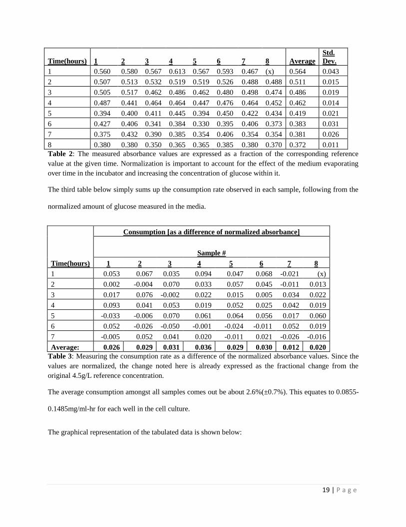
Table 2: The measured absorbance values are expressed as a fraction of the corresponding reference
value at the given time. Normalization is important to account for the effect of the medium evaporating
over time in the incubator and increasing the concentration of glucose within it.
The third table below simply sums up the consumption rate observed in each sample, following from the
normalized amount of glucose measured in the media.
Time(hours)
Consumption [as a difference of normalized absorbance]
Sample #
1 2 3 4 5 6 7 8
1 0.053 0.067 0.035 0.094 0.047 0.068 -0.021 (x)
2 0.002 -0.004 0.070 0.033 0.057 0.045 -0.011 0.013
3 0.017 0.076 -0.002 0.022 0.015 0.005 0.034 0.022
4 0.093 0.041 0.053 0.019 0.052 0.025 0.042 0.019
5 -0.033 -0.006 0.070 0.061 0.064 0.056 0.017 0.060
6 0.052 -0.026 -0.050 -0.001 -0.024 -0.011 0.052 0.019
7 -0.005 0.052 0.041 0.020 -0.011 0.021 -0.026 -0.016
Average: 0.026 0.029 0.031 0.036 0.029 0.030 0.012 0.020
Table 3: Measuring the consumption rate as a difference of the normalized absorbance values. Since the
values are normalized, the change noted here is already expressed as the fractional change from the
original 4.5g/L reference concentration.
The average consumption amongst all samples comes out be about 2.6%(±0.7%). This equates to 0.0855-
0.1485mg/ml-hr for each well in the cell culture.
The graphical representation of the tabulated data is shown below:
Page 25
20 | P a g e
Figure 2: The data shown in TABLE is shown here in compact form, representing the averaged
normalized absorbance value over time.
Cell density as counted using the Hemacytometer (Hausser Scientific, USA) was 418,000 cells/ml.
Calculating Cell consumption rate to use in the simulation:
Using the average consumption of 0.117 mg/ml (2.6% of 4.5g/L), and a cell count of 418,000
cells/ml, the consumption per cell is quantified as 4.0625x10⁻⁹
mg/ml-hr per cell. With chamber
dimensions in the bottom chamber of height 200 µm, a diameter of 770 µm, and an assumed spherical cell
shape in 3D culture with a radius of 10 µm, the number of cells that can be accommodated in the bottom
chamber at a seeding density of 50% is 8,420. The consumption rate for this number of cells in the
0.00705mm3 chamber volume is 9.50x10
-9g/L-s or 5.27210x10
-8 Kmol/m
3-s using the molar mass of
glucose as 180.0634g/mol. The reaction rates in ANSYS Fluent v.14 have to be implemented in units of
Kmol/m3-s.
The effects that are expected from the alteration of different parameters within the modeled
device fit the expectations approached from a qualitative intuition (with a few exceptions) ; however, the
quantitative values allows the placement of a scale to this intuitive disposition.
0.000
0.100
0.200
0.300
0.400
0.500
0.600
0.700
0 1 2 3 4 5 6 7 8 9
No
rmal
ize
d A
bso
rban
ce
Time (Hours)
Absorbance Value
Page 26
Section: Interpreting the Results
21 | P a g e
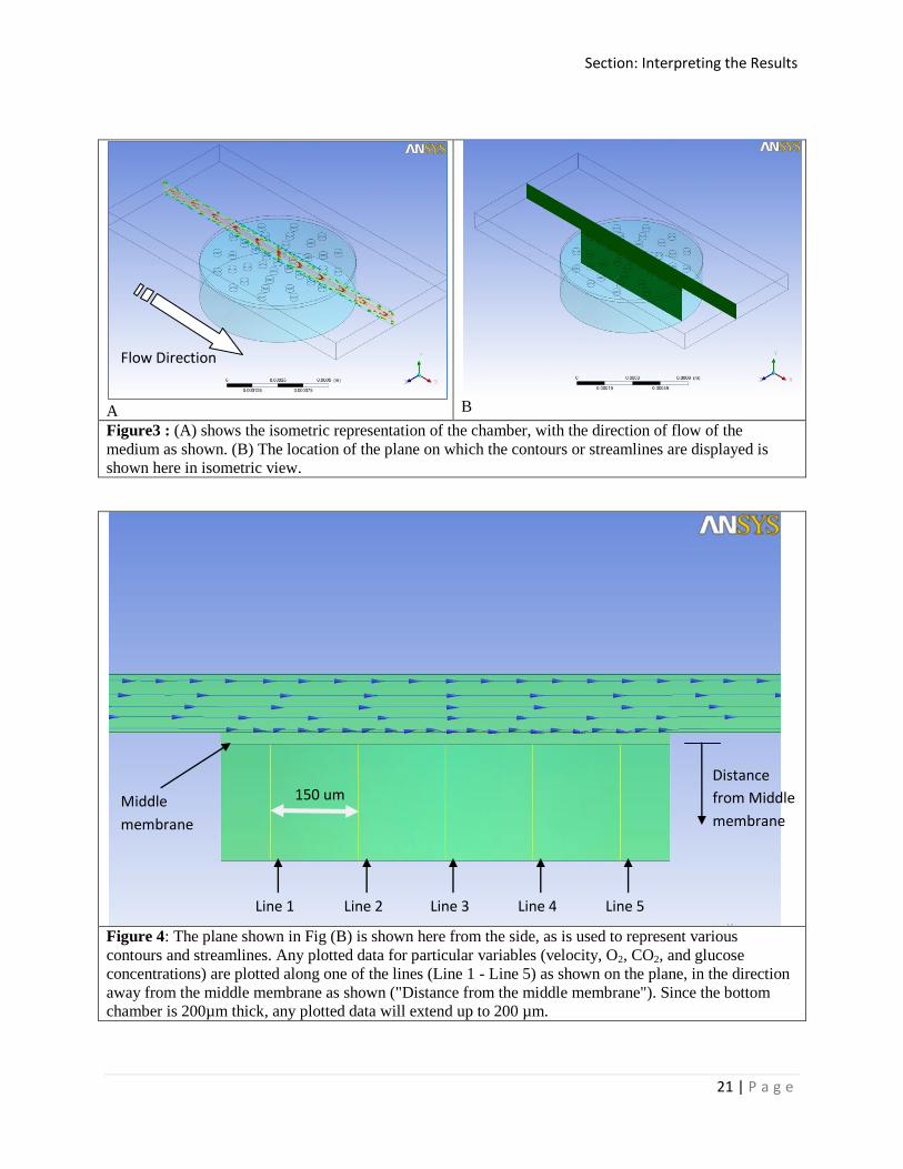
A B
Figure3 : (A) shows the isometric representation of the chamber, with the direction of flow of the
medium as shown. (B) The location of the plane on which the contours or streamlines are displayed is
shown here in isometric view.
Figure 4: The plane shown in Fig (B) is shown here from the side, as is used to represent various
contours and streamlines. Any plotted data for particular variables (velocity, O2, CO2, and glucose
concentrations) are plotted along one of the lines (Line 1 - Line 5) as shown on the plane, in the direction
away from the middle membrane as shown ("Distance from the middle membrane"). Since the bottom
chamber is 200µm thick, any plotted data will extend up to 200 µm.
Flow Direction
150 um Middle
membrane
Distance
from Middle
membrane
Line 5 Line 4 Line 3 Line 2 Line 1
Page 27
Section: Interpreting the Results
22 | P a g e
Representation of Data/Results
Note that the results shown in the figures below are either shown from an isometric viewpoint
(Fig. 3)or at the cross-section through the longitudinal axis of the device(with flow going from the left to
the right direction)as in Fig. 4. The graphs are plotted with data acquired along 5 lines through this cross-
section, spaced 150 µm apart between each pair, as also shown in Fig 4. The lines are labeled 1 through 5
progressively going from left to right (in the direction of flow). The data is plotted along the lines as we
move away from the middle membrane (shown in the figure as "Distance from middle membrane").
Page 28
Section: Changes in Pore Size
23 | P a g e
Changes in pore size
Figure 5: The streamlines along the plane is shown for dimensions: Pore Diameter of 40µm, membrane
thickness of 40µm, and a viscous resistance(hydrogel) of 5x10¹⁴
m-2
.
Figure 6: The contour along the plane is shown for dimensions: Pore Diameter of 40µm, membrane
thickness of 40µm, and a viscous resistance(hydrogel) of 5x10¹⁴
m-2
.
Figure 7: The streamlines along the plane is shown for dimensions: Pore Diameter of 20µm, membrane
thickness of 40µm, and a viscous resistance(hydrogel) of 5x10¹⁴
m-2
.
Page 29
Section: Changes in Pore Size
24 | P a g e
Figure 8 : The streamlines along the plane is shown for dimensions: Pore Diameter of 20µm, membrane
thickness of 40µm, and a viscous resistance(hydrogel) of 5x10¹⁴
m-2
.
Figure 9: The streamlines along the plane is shown for dimensions: Pore Diameter of 10µm, membrane
thickness of 40µm, and a viscous resistance(hydrogel) of 5x10¹⁴
m-2
.
Figure 10: The streamlines along the plane is shown for dimensions: Pore Diameter of 10µm, membrane
thickness of 40µm, and a viscous resistance(hydrogel) of 5x10¹⁴
m-2
.
Page 30
Section: Changes in Pore Size
25 | P a g e
Figure 11: The streamlines along the isometric view is shown for dimensions: Pore Diameter of 10µm,
membrane thickness of 40µm, and a viscous resistance(hydrogel) of 5x10¹⁴
m-2
.
Effect on streamlines: As the pore size is decreased from 40 µm to 10 µm, the flow becomes smoother –
almost a similar effect to that seen in lasers or optical fibers – the larger the length to width ratio of the
tube through with the laser or light passes, the more the likelihood of a collimated light beam coming out
at the output end. This effect is noticed by looking at the streamlines from Figs. 5, 7, and 9.
Page 31
Section: Changes in Pore Size
26 | P a g e
Figure 12: The velocity along Line 1 is shown for different pore sizes, membrane thickness of 40µm, and
a viscous resistance(hydrogel) of 5x10¹⁴
m-2
.
Effect on velocity profile
Reducing the pore size typically constrains the flow of fluid tangential to the main flow. If the
flow was directly fluxing through the middle layer only, then by the principles of momentum and mass
conservation (or even by Bernoulli's principle), the flow speed should increase with a decrease in pore
size. However, in the case where the fluid is taking a secondary flow path through the membrane pores
and hydrogel, the size of the pores positively correlate to the flow - the larger the pore size, the faster the
perfusion speed through the gel. The change is most significant between the 40 µm and 20 µm pore sizes
or between the 40 µm and 10 µm pore sizes. The range of velocities as seen from the data along Line 1
(Fig. 12) is as follows: 5.1x10⁻⁹
to 5.12x10⁻¹²
m/s for the 40 µm pore, 5.73x10⁻⁹
to 1.36x10⁻¹²
m/s for the
20 µm pore, and 3.67x10⁻⁹
to 2.10x10⁻¹²
m/s for the 10 µm pore. When the velocity is plotted on a log
1.00E-12
1.00E-11
1.00E-10
1.00E-09
1.00E-08
1
8
15
22
29
36
43
50
57
64
71
78
85
92
99
10
6
11
3
12
0
12
7
13
4
14
1
14
8
15
5
16
2
16
9
17
6
18
3
19
0
19
7
Vel
oci
ty M
agn
itu
de
(m/s
) [L
ogs
cale
]
Distance from middle membrane (µm)
10um Pore 20um Pore 40 um Pore
Page 32
Section: Changes in Pore Size
27 | P a g e
scale, the velocity gradients along the chamber depth for the different pore sizes show a similar profile
between 20 and 40 µm, but in terms of actual velocity magnitude, the 10 and 20 µm are closer on the log
scale. One noticeable point is that less than a depth of ~60 µm, the flow from the 20 µm pore is higher
than in the 10 µm pores, but after that this role switches with the 10 µm pore providing a slightly faster
flow.
Effect on oxygen concentration
The conditions created by using a 10 µm pore shows drastic results over the use of a 40 µm pore. With a
10 µm pore size, the chamber is seen to receive more oxygen than in the case of the 40 µm pore, by about
0.8% (Fig. 13) This is possibly due to the gas permeable membrane which is open to diffusion of oxygen,
and the comparatively “turbulent” flow in the 40 µm pore size device may drive against the diffusive
gradient of oxygen.
Figure 13: The O2 concentration along Line 1 is shown for 40 µm and 10 µm pore sizes, membrane
thickness of 40µm, and a viscous resistance(hydrogel) of 5x10¹⁴
m-2
Effect on Glucose Concentration
2.10E-06
2.20E-06
2.30E-06
2.40E-06
2.50E-06
2.60E-06
2.70E-06
2.80E-06
2.90E-06
1
8
15
22
29
36
43
50
57
64
71
78
85
92
99
10
6
11
3
12
0
12
7
13
4
14
1
14
8
15
5
16
2
16
9
17
6
18
3
19
0
19
7
O2
co
nce
ntr
atio
n (
g/g)
Distance from middle membrane (um)
40um pore 10um pore
Page 33
Section: Changes in Pore Size
28 | P a g e
The levels of glucose drop slightly in the 10 µm pore size compared to the 40 µm pore size structure. This
is expected as the flow is reduced in the smaller pore and glucose cannot diffuse through the gas
permeable middle membrane like O2 or CO2. The difference is about 0.5%.
Figure 14: The glucose concentration along Line 1 is shown for 40 µm and 10 µm pore sizes, membrane
thickness of 40µm, and a viscous resistance(hydrogel) of 5x10¹⁴
m-2
Effect on Carbon Dioxide Concentration:
The carbon dioxide profile shows a slightly higher concentration for the 10 µm pores compared to the 40
µm pores (by about 1.7%). This is most likely attributable to the slow flow through the medium, allowing
only diffusion to move the CO2 from the bottom of the chamber to the top. For the rather mixed, non-
streamed flow through the 40 µm pores, the CO2 can be delivered faster to the middle membrane from
where it can be convected and diffused out.
0.0005
0.00055
0.0006
0.00065
0.0007
0.00075
0.0008
0.00085
0.0009
1
8
15
22
29
36
43
50
57
64
71
78
85
92
99
10
6
11
3
12
0
12
7
13
4
14
1
14
8
15
5
16
2
16
9
17
6
18
3
19
0
19
7
Glu
cose
co
nce
ntr
atio
n (
g/g)
Distance from middle membrane (um)
40um pore 10um pore
Page 34
Section: Changes in Pore Size
29 | P a g e
Figure 15: The CO2 concentration along Line 1 is shown for 40 µm and 10 µm pore sizes, membrane
thickness of 40µm, and a viscous resistance(hydrogel) of 5x10¹⁴
m-2
0.00E+00
5.00E-08
1.00E-07
1.50E-07
2.00E-07
2.50E-07
3.00E-07
1
8
15
22
29
36
43
50
57
64
71
78
85
92
99
10
6
11
3
12
0
12
7
13
4
14
1
14
8
15
5
16
2
16
9
17
6
18
3
19
0
19
7 C
O2
co
nce
ntr
atio
n (
g/g)
Distance from middle membrane (um)
40um pore 10um pore
Page 35
Section: Changes in Membrane Thickness
30 | P a g e
Changes in middle membrane thickness (change in the pore depth)
Figure 16: The contour along the plane is shown for dimensions: Pore Diameter of 20µm, membrane
thickness of 40µm, and a viscous resistance(hydrogel) of 5x10¹⁴
m-2
.
Figure 17: The contour along the plane is shown for dimensions: Pore Diameter of 20µm, membrane
thickness of 30µm, and a viscous resistance(hydrogel) of 5x10¹⁴
m-2
.
Page 36
Section: Changes in Membrane Thickness
31 | P a g e
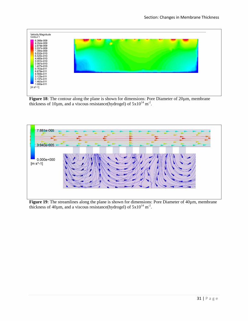
Figure 18: The contour along the plane is shown for dimensions: Pore Diameter of 20µm, membrane
thickness of 10µm, and a viscous resistance(hydrogel) of 5x10¹⁴
m-2
.
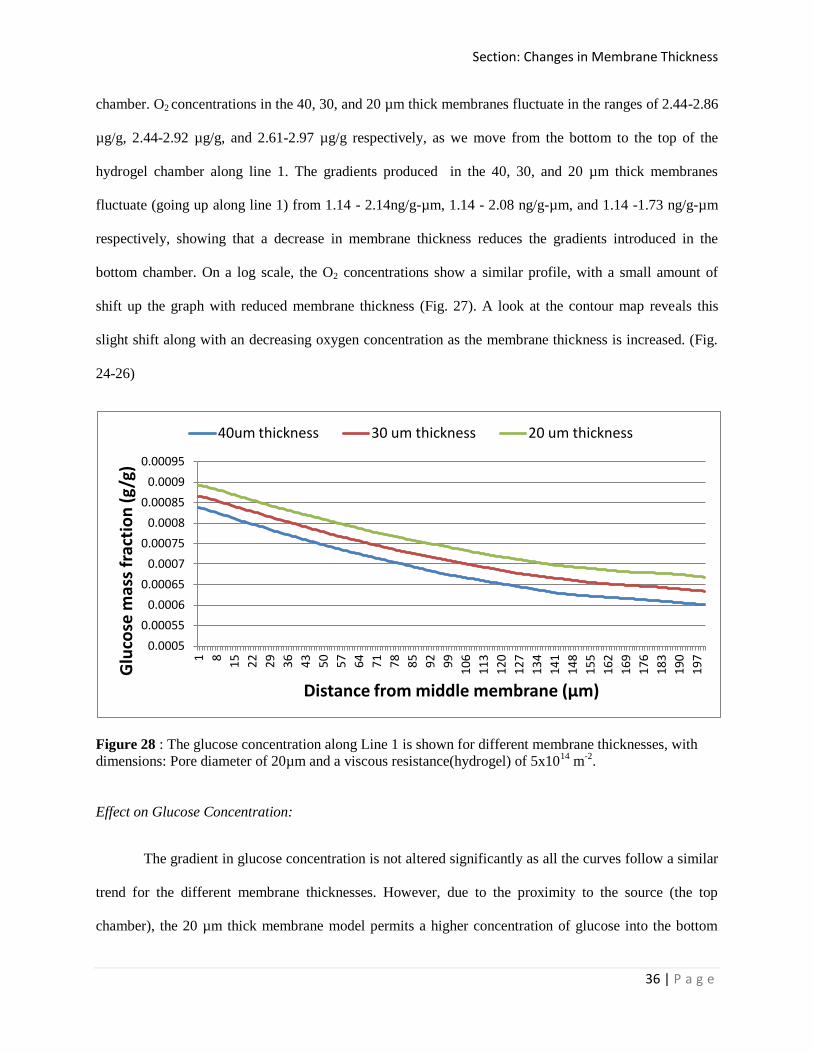
Figure 19: The streamlines along the plane is shown for dimensions: Pore Diameter of 40µm, membrane
thickness of 40µm, and a viscous resistance(hydrogel) of 5x10¹⁴
m-2
.
Page 37
Section: Changes in Membrane Thickness
32 | P a g e
Figure 20: The streamlines along the plane is shown for dimensions: Pore Diameter of 40µm, membrane
thickness of 30µm, and a viscous resistance(hydrogel) of 5x10¹⁴
m-2
.
Figure 21: The streamlines along the plane is shown for dimensions: Pore Diameter of 40µm, membrane
thickness of 20µm, and a viscous resistance(hydrogel) of 5x10¹⁴
m-2
.
Page 38
Section: Changes in Membrane Thickness
33 | P a g e
Figure 22: The streamlines along the plane is shown for dimensions: Pore Diameter of 40µm, membrane
thickness of 10µm, and a viscous resistance(hydrogel) of 5x10¹⁴
m-2
.
Effect on streamlines
The reduction of membrane thickness creates less divergence of the flow at the pore region,
creating a more streamlined flow through the bottom chamber (Fig. 19-22). This may not be clearly
evident in the case of 20 µm pores, but is clear in the 40 µm pores as the flow in the 40 µm thick middle
membrane shows a seemingly divergent pattern, as if there were 3 different regions of flow in the bottom
chamber (Fig. 19), which becomes more convergent as the membrane size is reduced as visualized in the
model with a 10 µm thick middle layer. (Fig. 22)
Figure 23: The velocity along Line 2 is shown for different membrane thicknesses, and dimensions: Pore
diameter of 20µm, and a viscous resistance(hydrogel) of 5x10¹⁴
m-2
.
1.00E-12
1.00E-11
1.00E-10
1.00E-09
1.00E-08
1.00E-07
1.00E-06
1
8
15
22
29
36
43
50
57
64
71
78
85
92
99
10
6
11
3
12
0
12
7
13
4
14
1
14
8
15
5
16
2
16
9
17
6
18
3
19
0
19
7
Ve
loci
ty m
agn
itu
de
(m
/s)
[Lo
gsca
le]
Distance from middle membrane (µm)
40 um Membrane 30 um Membrane 20 um Membrane
Page 39
Section: Changes in Membrane Thickness
34 | P a g e
Effect on velocity profile
The velocity profile depicts that the flow conditions with the thicker middle membranes (30 µm
and 40 µm) are almost just a shifted version of the flow through the 20µm thick membrane (using data
from line 2, Fig. 23), shifted by the same amount that the membrane size is reduced by with each case (10
µm). This is true in flows that are relatively similar in profile (in this case, the 20 µm pore size creates a
nice streamed flow, as opposed to the 40 µm pores.) It is observed that any given location will have a
higher net velocity if the membrane thickness is reduced.
A
Figure 24: The contour along the plane is shown for dimensions: Pore diameter of 20µm, membrane
thickness of 40µm, and a viscous resistance(hydrogel) of 5x10¹⁴
m-2
.
B
Figure 25: The contour along the plane is shown for dimensions: Pore diameter of 20µm, membrane
thickness of 30µm, and a viscous resistance(hydrogel) of 5x10¹⁴
m-2
.
Page 40
Section: Changes in Membrane Thickness
35 | P a g e
C
Figure 26: The contour along the plane is shown for dimensions: Pore diameter of 20µm, membrane
thickness of 20µm, and a viscous resistance(hydrogel) of 5x10¹⁴
m-2
.
Figure 27: The oxygen concentration along Line 1 is shown for different membrane thicknesses, with
dimensions: Pore diameter of 20µm and a viscous resistance(hydrogel) of 5x10¹⁴
m-2
. The graph is not
entirely smooth, perhaps due to discretization of elements within the model.
Effect on oxygen concentration
O2 concentration overall increases while the gradient decreases when the membrane thickness is
reduced. This is intuitive as the bottom chamber is brought closer to the source of the flow in the top
2.00E-06
2.20E-06
2.40E-06
2.60E-06
2.80E-06
3.00E-06
3.20E-06
1
8
15
22
29
36
43
50
57
64
71
78
85
92
99
10
6
11
3
12
0
12
7
13
4
14
1
14
8
15
5
16
2
16
9
17
6
18
3
19
0
19
7
O2
mas
s fr
acti
on
(g/
g)
Distance from middle membrane (µm)
40um thickness 30 um thickness 20 um thickness
Page 41
Section: Changes in Membrane Thickness
36 | P a g e
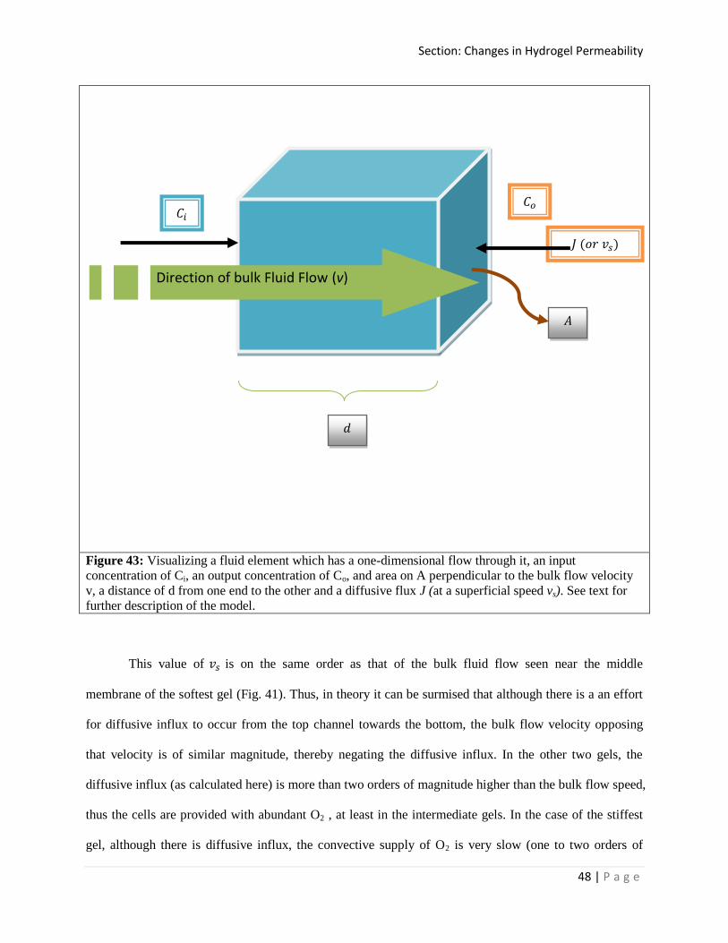
chamber. O2 concentrations in the 40, 30, and 20 µm thick membranes fluctuate in the ranges of 2.44-2.86
µg/g, 2.44-2.92 µg/g, and 2.61-2.97 µg/g respectively, as we move from the bottom to the top of the
hydrogel chamber along line 1. The gradients produced in the 40, 30, and 20 µm thick membranes
fluctuate (going up along line 1) from 1.14 - 2.14ng/g-µm, 1.14 - 2.08 ng/g-µm, and 1.14 -1.73 ng/g-µm
respectively, showing that a decrease in membrane thickness reduces the gradients introduced in the
bottom chamber. On a log scale, the O2 concentrations show a similar profile, with a small amount of
shift up the graph with reduced membrane thickness (Fig. 27). A look at the contour map reveals this
slight shift along with an decreasing oxygen concentration as the membrane thickness is increased. (Fig.
24-26)
Figure 28 : The glucose concentration along Line 1 is shown for different membrane thicknesses, with
dimensions: Pore diameter of 20µm and a viscous resistance(hydrogel) of 5x10¹⁴
m-2
.
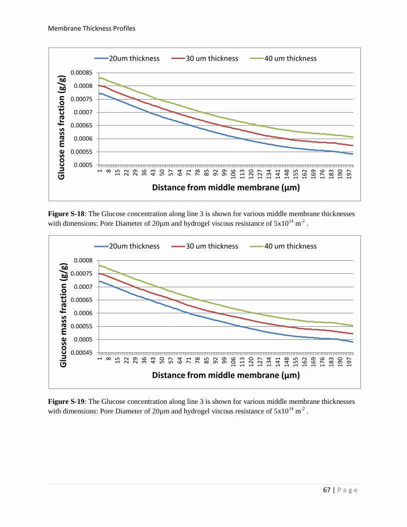
Effect on Glucose Concentration:
The gradient in glucose concentration is not altered significantly as all the curves follow a similar
trend for the different membrane thicknesses. However, due to the proximity to the source (the top
chamber), the 20 µm thick membrane model permits a higher concentration of glucose into the bottom
0.0005
0.00055
0.0006
0.00065
0.0007
0.00075
0.0008
0.00085
0.0009
0.00095
1
8
15
22
29
36
43
50
57
64
71
78
85
92
99
10
6
11
3
12
0
12
7
13
4
14
1
14
8
15
5
16
2
16
9
17
6
18
3
19
0
19
7
Glu
cose
mas
s fr
acti
on
(g/
g)
Distance from middle membrane (µm)
40um thickness 30 um thickness 20 um thickness
Page 42
Section: Changes in Membrane Thickness
37 | P a g e
chamber, with a lower concentration in the 30 µm thick membrane, and the lowest being in the 40 µm
thick membrane. The ranges for each of these models, respectively, are: 606-831 µg/g, 574-802 µg/g and
542-772 µg/g along the data on Line 1 (Fig. 28).
Figure 29: The CO2 concentration along Line 1 is shown for different membrane thicknesses, with
dimensions: Pore diameter of 20µm and a viscous resistance(hydrogel) of 5x10¹⁴
m-2
.
Effect on Carbon Dioxide Concentration
The gradient in the CO2 concentration drops slightly with decreasing membrane thickness
(<0.1%), but is otherwise considerably unaltered within the different membrane thickness samples. The
actual concentration profiles are simply shifted versions of similar curves (Fig. 29). The concentration of
CO2 goes up with membrane thickness, using data from FIGURE (line 3), the concentration range for
CO2 in the 40, 30, and 20 µm pore sizes are 185-302 ng/g, 176-293 ng/g, 166-284 ng/g respectively. The
ranges depict that reduced membrane thickness also reduces the range of CO2 produced in the bottom
chamber, thus creating a reduced gradient (although the change is <0.1%).
0.00E+00
5.00E-08
1.00E-07
1.50E-07
2.00E-07
2.50E-07
3.00E-07
1
8
15
22
29
36
43
50
57
64
71
78
85
92
99
10
6
11
3
12
0
12
7
13
4
14
1
14
8
15
5
16
2
16
9
17
6
18
3
19
0
19
7
CO
2 m
ass
frac
tio
n (
g/g)
Distance from middle membrane (µm)
40um thickness 30 um thickness 20 um thickness
Page 43
Section: Changes in Hydrogel Permeability
38 | P a g e
Changes in hydrogel permeability
Figure 30: The streamlines along the plane is shown for dimensions: Pore diameter of 40µm, membrane
thickness of 40µm, and a viscous resistance(hydrogel) of 5x10¹⁴
m-2
.
Figure 31: The streamlines along the plane is shown for dimensions: Pore diameter of 40µm, membrane
thickness of 40µm, and a viscous resistance(hydrogel) of 5x10¹²
m-2
.
Effect on streamlines
In the example shown with membranes of 40 µm thickness and 40 µm pore sizes(Fig. 30) it is
noticed that the stiffest hydrogel (viscous resistance of 5 x 10¹⁴
m-2
) provides the least compliance to the
fluid flow through the gel - the flow is almost divided into separate regions or apparent vortices as viewed
Page 44
Section: Changes in Hydrogel Permeability
39 | P a g e
from the cross-section. As the gel is made more permeable towards a viscous resistance of 5 x 10¹²
m-2
,
the flow becomes less diverged. (Fig. 31)
Figure 32: The velocity along Line 1 is shown for different gel stiffnesses, with dimensions: Pore
diameter of 20µm, membrane thickness of 40µm, and a viscous resistance(hydrogel) of 5x10¹⁴
m-2
.
Effect on velocity profile
As the permeability increases, the net velocity magnitude fluxing through the chamber (with
hydrogel) also increases. This should generally be the case, as in the extreme case of no resistance
(infinite permeability, i.e., no hydrogel but only the original liquid phase of the perfusing medium), there
would be no retardation to the flow through the bottom chamber. The increase in permeability by one
order of magnitude typically raises the velocity by about one order of magnitude as well. Looking
specifically at the data from (Fig. 32), at line 1, the velocity in the stiffest gel is on the order of 10-5
to 10-
4 µm/sec at about 15 - 190 µm away from the middle membrane. In the intermediate gel, this range speeds
up to 10-4
to 10-3
µm/sec, and to 10-3
to 10-2
µm/sec in the softest gel. A similar shift in the order of
magnitude can be seen at the data along all locations (lines). At the middle of the bottom chamber (along
1.00E-12
1.00E-11
1.00E-10
1.00E-09
1.00E-08
1.00E-07
1.00E-06 1
8
15
22
29
36
43
50
57
64
71
78
85
92
99
10
6
11
3
12
0
12
7
13
4
14
1
14
8
15
5
16
2
16
9
17
6
18
3
19
0
19
7
Ve
loci
ty m
agn
itu
de
(m
/s)
[Lo
gsca
le]
Distance from middle membrane (µm)
Stiffest Gel (Visc. Res: 5e+14) Intermediate Gel (Visc Res: 5e+13) Softest Gel (Visc Res: 5e+12)
Page 45
Section: Changes in Hydrogel Permeability
40 | P a g e
line 3), the average speed is on the order of 10-4
, 10-3
,10-2
µm/sec respectively for the stiffest, intermediate,
and softest gel respectively.
Figure 33: The contours along the plane is shown for dimensions: Pore Diameter of 20µm, membrane
thickness of 30µm, and a viscous resistance(hydrogel) of 5x10¹⁴
m-2
.
Figure 34: The contours along the plane is shown for dimensions: Pore Diameter of 20µm, membrane
thickness of 30µm, and a viscous resistance(hydrogel) of 5x10¹³
m-2
.
Page 46
Section: Changes in Hydrogel Permeability
41 | P a g e
Figure 35: The streamlines along the plane is shown for dimensions: Pore Diameter of 20µm, membrane
thickness of 30µm, and a viscous resistance(hydrogel) of 5x10¹²
m-2
.
Figure 36: The velocity along Line 1 is shown for different gel stiffnesses, with dimensions: Pore
diameter of 20µm, membrane thickness of 30µm.
Effect on oxygen concentration
The results for the oxygen profile is rather counterintuitive when compared across gels of
different stiffness Fig. 33-35. Following along the data on line 1,(Fig. 36)the gradient follows a similar
trend across all locations - for the first 40 µm from the surface of the middle membrane, the gradient in O2
concentration (as a mass fraction, µg/g) gradient is about 0.003 µg/g-µm. This gradient drops to 0.0025
µg/g-µm over the next 40 µm(40 - 80 µm) , to 0.002 µg/g-µm over the next 40 µm (80 - 120 µm), to
0.0017 µg/g-µm over the next 10 µm (120-130 µm) and to about 0.0013 µg/g-µm from 130 µm on
downwards. This trend is seen in all three gels, however, the trend for the softest gel slightly varies after
130 µm in depth, where the gradient drops to about 0.001 µg/g-µm from 130 -150 µm depth, to 0.0007
from 150 - 170 µm depth, and about 0.0004 µg/g-µm in the remainder of the chamber. Although the
gradients are more similar in the stiffest and intermediate gels, the actual concentration of O2 in the
simulated gels show a closer resemblance between the stiffest and softest gels than the intermediate gel,
2.20E-06
2.30E-06
2.40E-06
2.50E-06
2.60E-06
2.70E-06
2.80E-06
2.90E-06
3.00E-06
3.10E-06 1
8
15
22
29
36
43
50
57
64
71
78
85
92
99
10
6
11
3
12
0
12
7
13
4
14
1
14
8
15
5
16
2
16
9
17
6
18
3
19
0
19
7
Oxy
gen
mas
s fr
acti
on
(g/
g)
Distance from middle membrane (µm)
Stiffest Gel (Visc. Res: 5e+14) Intermediate Gel (Visc Res: 5e+13) Softest Gel (Visc Res: 5e+12)
Page 47
Section: Changes in Hydrogel Permeability
42 | P a g e
with the intermediate gel having the highest O2 concentration. Looking along the data on line 1 (Fig. 36),
the range of O2 concentration for the stiffest and intermediate are 2.53 - 2.92 µg/g and 2.70 - 2.99 µg/g
respectively, seeming to convey the idea that the better perfusion (higher velocities) in the intermediate
gel allows better transport of oxygen into the chamber. In the softest gel, however, the velocity profiles
are the highest compared to the other two gels, but the O2 concentration drops back drops back to 2.53 -
2.91 µg/g, very similar to that in the stiffest gel.
Figure 37: The glucose concentration along Line 1 is shown for different gel stiffnesses, with dimensions:
Pore diameter of 20µm, membrane thickness of 30µm.
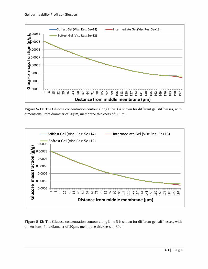
Effect on Glucose Concentration
The glucose concentration shows a very replicated similarity between the gels, unlike the oxygen
and carbon dioxide profiles. Along line 3, for instance, the range for the stiffest and intermediate gels are
0.574 - 0.802 mg/g and 0.573 - 0.801respectively, while a higher range of 0. 583-0.803 mg/g is seen in
the softest gel. This relatively identical profile in all three different gels suggest that due to the abundance
of glucose, its concentration is not affected by the flow rate, it is a reaction that is diffusion-dominated,
where the diffusion is sufficient to overcome its consumption rate.
0.0006
0.00065
0.0007
0.00075
0.0008
0.00085
0.0009
1
8
15
22
29
36
43
50
57
64
71
78
85
92
99
10
6
11
3
12
0
12
7
13
4
14
1
14
8
15
5
16
2
16
9
17
6
18
3
19
0
19
7
Glu
cose
mas
s fr
acti
on
(g/
g)
Distance from middle membrane (µm)
Stiffest Gel (Visc. Res: 5e+14) Intermediate Gel (Visc Res: 5e+13) Softest Gel (Visc Res: 5e+12)
Page 48
Section: Changes in Hydrogel Permeability
43 | P a g e
Figure 38: The CO2 concentration along Line 1 is shown for different gel stiffnesses, with dimensions:
Pore diameter of 20µm, membrane thickness of 30µm.
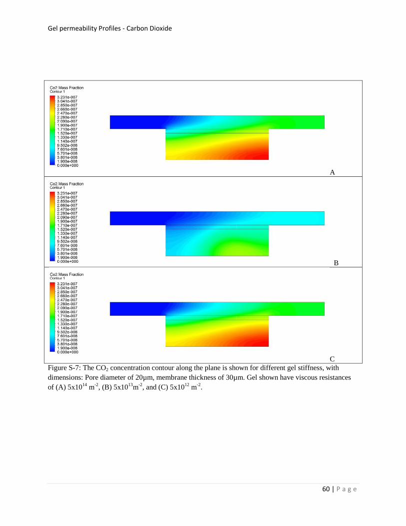
Effect on Carbon Dioxide Concentration
The carbon dioxide generated in the chamber again shows a similarity between the stiffest and
softest gels. Comparing along the data in line 3 (Fig. 3), the range in these two gels are 176 -293 ng/g and
176 - 294 ng/g respectively. In the intermediate gel, this range decreases (presumably due to better
perfusion) to 92 - 174 ng/g, which is outside of the range of either the stiffest or softest gels.
The unexpected case
The unusual O2 and CO2 pattern noticed with the change in permeability warrants some
discussion. The velocity magnitude by itself shows an increase as the permeability increases, as better
perfusion by virtue of increased velocity is seen in the glucose concentration being the highest in the
softest gel. Glucose, however, is an abundant resource in the media (1mg/g) and is not a limiting factor
for cell metabolic rates. O2, due to its low solubility, defines the metabolic limitations more so than
glucose (0.2mmol/L or approximately 3.2mg/g). Having the media perfusing at a faster velocity through
the gel may lead to the thought that the O2 will be better delivered by convection, which supplements the
0.00E+00
5.00E-08
1.00E-07
1.50E-07
2.00E-07
2.50E-07
3.00E-07
1
8
15
22
29
36
43
50
57
64
71
78
85
92
99
10
6
11
3
12
0
12
7
13
4
14
1
14
8
15
5
16
2
16
9
17
6
18
3
19
0
19
7
CO
2 m
ass
frac
tio
n (
g/g)
Distance from middle membrane (µm)
Stiffest Gel (Visc. Res: 5e+14) Intermediate Gel (Visc Res: 5e+13)
Softest Gel (Visc Res: 5e+12)
Page 49
Section: Changes in Hydrogel Permeability
44 | P a g e
already present diffusion of O2 into the bottom chamber. Although this seems to hold true when
comparing the stiffest and intermediate gels, the same does not hold true for the softest gel.
To explain this unexpected phenomenon, a contour of the net velocity magnitude (Figs. 39,40)and
the positive (upwards) y-direction velocity component (Figs. 41,42)may provide a better insight into the
problem. The y-component of the stiffest gel is not shown because only the velocity range between 7x10⁻⁹
and 10-7
m/s is sought, but from the net magnitude contour of the stiffest gel in Fig. 40, it is easy to see
that those values will be out of range.
A
B
Figure 39: Velocity magnitude profiles in the range of 10-8
m/s to 5.4x10⁻⁷
m/s in the bottom chamber
with viscous resistances of (A) 5x10¹²
m-2
, and (B) 5x10¹²
m-2
. Both cases have same chamber
dimensions: 20 µm pore size, 30 µm membrane thickness.
Page 50
Section: Changes in Hydrogel Permeability
45 | P a g e
Figure 40: Velocity magnitude profiles in the range of 10-12
m/s to 5.4x10⁻⁹
m/s in the bottom chamber
with a viscous resistance of 5x10¹⁴
m-2
. The dimensions are the same as the chambers in Fig. 39 (20 µm
pore size, 30 µm membrane thickness). Note that the velocity magnitude in this system is well out of an
order of magnitude of the systems in Fig. 39 (the intermediate and softer gel).
Figure 41: Another look at velocity in the chamber with the softest gel. This time, only the positive y-
direction (upwards) velocity is shown, in the range of 10-9
m/s to 5.4x10⁻⁷
m/s. The chamber dimensions
are still at a 20 µm pore size and a 30 µm membrane thickness.
Page 51
Section: Changes in Hydrogel Permeability
46 | P a g e
Figure 42: Positive y-velocity components in the chamber with the intermediate gel, in the range of 10-9
m/s to 5.4x10⁻⁷
m/s. The chamber dimensions are still at a 20 µm pore size and a 30 µm membrane
thickness.
The range is shown only on the order of 0.01-0.1 µm/sec. As is clear from the contour, this
velocity regime is only existent in close to the middle membrane for the softest gel, while such a
relatively high velocity profile is absent from the other two gels. One way to explain this is the lack of
diffusive support in the softest gel by employing Fick's Law of Diffusion. Using a typical fluid element to
analyze the factors affecting diffusion and flow (Fig. 43), the following assumptions and conventions for
the analysis of the element are made:
(1) The problem is one-dimensional: the velocity components are only in one direction (in the x-direction),
and diffusion can happen only along this direction as well.
(2) The velocity entering the fluid element is the same as the velocity exiting the element (mass
conservation principle with no mass accumulation within the fluid element).
(3) The concentration at the input side is and at the output side it is .
Page 52
Section: Changes in Hydrogel Permeability
47 | P a g e
(4) - )
(5) The area through which the fluid is fluxing in or out is called , while the thickness of the fluid
element is d.
(6) The diffusivity of the species is D.
(7) J is the diffusive flux of the species (in units of g/m2-s)
Using the above conventions, Fick's Law of Diffusion can be written as:
, where we can approximate to the first order that
.
The net flux in mass is:
. But the net flux can also be defined by a superficial velocity of the
species itself. The species (in this case, O2) has a certain concentration immediately outside of the fluid
element (at ), and the flux into the element cannot be higher than the number of species particles that
can provide. Thus, if we assume there is a superficial species "velocity" - which is the velocity vs
required at which, given a concentration of , the flux will match the value of : .
In other words:
,
which simplifies to:
. Since , we can just consider the magnitude of the velocity:
An order of magnitude analysis on this equation uses the following assumptions for the fluid element:
These values give:
.
Page 53
Section: Changes in Hydrogel Permeability
48 | P a g e
Figure 43: Visualizing a fluid element which has a one-dimensional flow through it, an input
concentration of Ci, an output concentration of Co, and area on A perpendicular to the bulk flow velocity
v, a distance of d from one end to the other and a diffusive flux J (at a superficial speed vs). See text for
further description of the model.
This value of is on the same order as that of the bulk fluid flow seen near the middle
membrane of the softest gel (Fig. 41). Thus, in theory it can be surmised that although there is a an effort
for diffusive influx to occur from the top channel towards the bottom, the bulk flow velocity opposing
that velocity is of similar magnitude, thereby negating the diffusive influx. In the other two gels, the
diffusive influx (as calculated here) is more than two orders of magnitude higher than the bulk flow speed,
thus the cells are provided with abundant O2 , at least in the intermediate gels. In the case of the stiffest
gel, although there is diffusive influx, the convective supply of O2 is very slow (one to two orders of
Direction of bulk Fluid Flow (v)
Page 54
Section: Changes in Hydrogel Permeability
49 | P a g e
magnitude less than that in the intermediate gel). This means that in this gel, it can take about 10-100 fold
of the time that it takes in the intermediate gel to supply O2 to the cells in the hydrogel convectively,
making this situation heavily diffusion-driven. In the softest gel, the convective component is there, but
the diffusive component is missing. It would appear that the intermediate gel provides a more adequate
balance between convective and diffusive supply of O2.
Page 55
50 | P a g e
4. Conclusion
This study was conducted in order to understand the way that altering parameters will change
flow and diffusive behavior in the microchamber. There are many parameters that can be tuned, and
whether the optimum conditions specific to the requirements of the user can be chosen can determine
what parameters to specify the device manufacture to. The validity of the simulation should be verified in
a few models by use of various markers (for pO2, pH, glucose) [14, 21, 22] and techniques such as
fluorescence recovery after photobleaching (FRAP). [23]
The data obtained can be advantageous in terms of design considerations. For instance, changing
the permeability in the bottom chamber by change of the viscous resistance from 5x10¹⁴
m-2
to 5x10¹³
m-2
gives a faster flow and better delivery of oxygen as expected, but in making the gel even softer to a
viscous resistance of 5x10¹²
m-2
, the oxygen content drops back to the same conditions as that in the
stiffest gel. Thus, the intermediate gel shows the best perfusion and delivery of oxygen out of the three
permeabilities. This allows us to use this as a tool to provide the same oxygenated conditions just by
alteration of the hydrogel's permeability to the correct degree. For our case, we can change the peptide
percentage of PuraMatrix to tune the gel permeability. Tumor cells can respond to flow, and has
competing mechanisms to go against or with the flow. [24] To be able to generate two diverse flow
conditions while keeping nutrient amounts the same (such as glucose), it is possible to study the isolated
effect of flow on the cultured cells without the need to regulate the amount of oxygen supplied in the
perfusing medium to ensure the same oxygenated conditions.[25, 26]
The typical interstitial fluid flow is on the order of 0.1-2 µm/sec. One such case in which this
flow speed is achieved is when the viscous resistance is at 5x10¹²
m-2
. In the other permeabilities, the fluid
convection speed is very low, on the order of 10-3
to 10-6
µm/sec. That does not invalidate these models
for use as cell culture. Cancer cells typically harbor a microenvironment marked by high interstitial fluid
pressure and very low fluid flow due to the lack of functional lymphatics. [8] Studies show that
Page 56
51 | P a g e
normalizing the capillary structure and repairing the lymphatic architecture allows drugs to perfuse better
into the cancer cells as well as a slightly better prognosis (about 6 months). The microvessels surrounding
a solid tumor, however, is very permeable. This situation can be studied in the microchamber by using a
large pore size (40 µm) and high viscous resistance of the hydrogel (5x10¹⁴
m-2
). The same study can be
performed on a smaller pore size (20 µm) with the same or different permeability to see the effect of a
reduced permeability only in the middle membrane (not in the solid tumor, which is represented by the
hydrogel). In terms of clinical application, using biopsy samples instead of cell cultures, one could test
whether altering the different parameters will affect the tumor cells and aid in drug screening and give an
insight into whether altering those parameters in the physiology of the patient will truly have an effect on
the cancer cells, including conditions not mentioned in this study (such as hyperthermia) that can be used
in conjunction with the microfluidic device to test for the synergistic effects of multiple stimuli.[26-28]
By having a chart representative of the conditions induced in the microchamber through the use of CFD,
the observed experimental results can be explained in conjunction with them.
Page 57
52 | P a g e
5. Summary
In this study, a few characteristics in the CFD model of the original 3D LCA device has been
altered to note the changes introduced in the microchamber due to these alterations. In general, the trend
found was that: (1) velocities correlate positively with changes in pore size and permeability, and
inversely correlates with membrane thickness; (2) the glucose profile remains unchanged based on
permeability, but does increase with an increase in pore size or a decrease in membrane thickness. For
instance, if a stiff microenvironment needs to be simulated in the real device, based on the simulation
results, it would be optimal to use 20 µm pore sizes for smooth, streamlined flow but with a membrane
thickness of only 20 µm so that velocities on the order similar to the interstitial fluid flow can be reached
(~ 0.1 µm/sec). The profile for CO2 has a very high inverse correlation to the O2 profile, thus, based on
the simulation results, knowing one may help estimate the other. This is not the case for glucose as there
is a situation where there is an almost identical glucose profile (for different permeabilities) but very
different O2 and CO2 profiles. Using only experience and physiological revelations to guide the design of
the device may not necessarily give the expected profile within the microchamber, and CFD can step in to
provide the insight that can also motivate the design towards an optimal direction without relying on trial-
and-error methods of optimization.
Page 58
53 | P a g e
6. References:
1. Anderson, J., Computational Fluid Dynamics. 1995: McGraw-Hill Science/Engineering/Math.
2. Palsson, B.O. and S.N. Bhatia, Tissue Engineering. 2004: Pearson Prentice Hall.
3. Martin, Y. and P. Vermette, Bioreactors for tissue mass culture: design, characterization, and
recent advances. Biomaterials, 2005. 26(35): p. 7481-503.
4. Brown, J.M. and A.J. Giaccia, The unique physiology of solid tumors: opportunities (and
problems) for cancer therapy. Cancer Res, 1998. 58(7): p. 1408-16.
5. Fukumura, D. and R.K. Jain, Tumor microenvironment abnormalities: causes, consequences, and
strategies to normalize. J Cell Biochem, 2007. 101(4): p. 937-49.
6. Gillies, R.J., et al., Causes and effects of heterogeneous perfusion in tumors. Neoplasia, 1999.
1(3): p. 197-207.
7. Iyer, A.K., et al., Exploiting the enhanced permeability and retention effect for tumor targeting.
Drug Discovery Today, 2006. 11(17–18): p. 812-818.
8. Baronzio, G., Fiorentini, G, Cogle, C.R, Cancer Microenvironment and Therapeutic Implications,
2009.
9. Lorusso, G. and C. Ruegg, The tumor microenvironment and its contribution to tumor evolution
toward metastasis. Histochem Cell Biol, 2008. 130(6): p. 1091-103.
10. Moulder, J.E. and S. Rockwell, Tumor hypoxia: its impact on cancer therapy. Cancer Metastasis
Rev, 1987. 5(4): p. 313-41.
11. Tredan, O., et al., Drug resistance and the solid tumor microenvironment. J Natl Cancer Inst,
2007. 99(19): p. 1441-54.
12. Graeber, T.G., et al., Hypoxia-mediated selection of cells with diminished apoptotic potential in
solid tumours. Nature, 1996. 379(6560): p. 88-91.
13. Zhong, H., et al., Overexpression of hypoxia-inducible factor 1alpha in common human cancers
and their metastases. Cancer Res, 1999. 59(22): p. 5830-5.
14. Gillies, R.J., et al., MRI of the tumor microenvironment. J Magn Reson Imaging, 2002. 16(4): p.
430-50.
15. Zeynep Dereli-Korkut, D.A., A.H.R. Ahmed, Xuejun Jiang, and Sihong Wang, Three
Dimensional Microfluidic Cell Arrays Mimicking Tumor Microenvironment. Lab on a Chip, (in
revision).
16. Swartz, M.A. and M.E. Fleury, Interstitial flow and its effects in soft tissues. Annu Rev Biomed
Eng, 2007. 9: p. 229-56.
17. Patrachari, A.R., J.T. Podichetty, and S.V. Madihally, Application of computational fluid
dynamics in tissue engineering. J Biosci Bioeng, 2012. 114(2): p. 123-32.
18. Fogler, S., Elements of Chemical Reaction Engineering (4th Edition). 2005: Prentice Hall.
19. Howat, W.J., et al., Basement membrane pores in human bronchial epithelium: a conduit for
infiltrating cells? Am J Pathol, 2001. 158(2): p. 673-80.
20. Takahashi-Iwanaga, H., T. Iwanaga, and H. Isayama, Porosity of the epithelial basement
membrane as an indicator of macrophage-enterocyte interaction in the intestinal mucosa. Arch
Histol Cytol, 1999. 62(5): p. 471-81.
21. Jain, R.K., L.L. Munn, and D. Fukumura, Dissecting tumour pathophysiology using intravital
microscopy. Nat Rev Cancer, 2002. 2(4): p. 266-76.
22. Nakasone, E.S., et al., Imaging tumor-stroma interactions during chemotherapy reveals
contributions of the microenvironment to resistance. Cancer Cell, 2012. 21(4): p. 488-503.
23. Periasamy, A. and A.P.S. . Methods in Cellular Imaging. 2001: American Physiological Society.
24. Polacheck, W.J., J.L. Charest, and R.D. Kamm, Interstitial flow influences direction of tumor cell
migration through competing mechanisms. Proceedings of the National Academy of Sciences,
2011.
25. Ng, C.P., C.L. Helm, and M.A. Swartz, Interstitial flow differentially stimulates blood and
lymphatic endothelial cell morphogenesis in vitro. Microvasc Res, 2004. 68(3): p. 258-264.
Page 59
54 | P a g e
26. Yu, H., J.K. Mouw, and V.M. Weaver, Forcing form and function: biomechanical regulation of
tumor evolution. Trends Cell Biol, 2011. 21(1): p. 47-56.
27. Ruoslahti, E., S.N. Bhatia, and M.J. Sailor, Targeting of drugs and nanoparticles to tumors. The
Journal of Cell Biology, 2010. 188(6): p. 759-768.
28. Song, C.W., et al., Implications of increased tumor blood flow and oxygenation caused by mild
temperature hyperthermia in tumor treatment. Int J Hyperthermia, 2005. 21(8): p. 761-7.
Page 60
55 | P a g e
7.Supplemental Figures:
This section is intended only to supplement the data in this study, and the study can be read independently
of this section. It showcases some of the other profiles from the same conditions that were not shown in
the study (from varying locations).
Page 61
Gel permeability Profiles - Velocity
56 | P a g e
Figure S-1: The streamlines along the plane is shown for dimensions: Pore Diameter of 20µm, membrane
thickness of 30µm, and a viscous resistance(hydrogel) of 5x10¹⁴
m-2
.
Figure S-2: The streamlines along the plane is shown for dimensions: Pore Diameter of 20µm, membrane
thickness of 30µm, and a viscous resistance(hydrogel) of 5x10¹³
m-2
.
Page 62
Gel permeability Profiles - Velocity
57 | P a g e
Figure S-3: The streamlines along the plane is shown for dimensions: Pore Diameter of 20µm, membrane
thickness of 30µm, and a viscous resistance(hydrogel) of 5x10¹³
m-2
Page 63
Gel permeability Profiles - Velocity
58 | P a g e
Figure S-4: The velocity along line 3 is shown for various stiffnesses of gels with dimensions: Pore
Diameter of 20µm and membrane thickness of 30µm.
Figure S-5: The velocity along line 5 is shown for various stiffnesses of gels with dimensions: Pore
Diameter of 20µm and membrane thickness of 30µm.
1.00E-12
1.00E-10
1.00E-08
1.00E-06
1.00E-04
1.00E-02
1.00E+00
1
8
15
22
29
36
43
50
57
64
71
78
85
92
99
10
6
11
3
12
0
12
7
13
4
14
1
14
8
15
5
16
2
16
9
17
6
18
3
19
0
19
7
Ve
loci
ty m
agn
itu
de
(m
/s)
[Lo
gsca
le]
Distance from middle membrane (µm)
Stiffest Gel (Visc. Res: 5e+14) Intermediate Gel (Visc Res: 5e+13) Softest Gel (Visc Res: 5e+12)
Page 64
Gel permeability Profiles - Oxygen
59 | P a g e
Figure S-5: The O2 concentration along line 3 is shown for various stiffnesses of gels with dimensions:
Pore Diameter of 20µm and membrane thickness of 30µm.
Figure S-6: The O2 concentration along line 5 is shown for various stiffnesses of gels with dimensions:
Pore Diameter of 20µm and membrane thickness of 30µm.
2.10E-06
2.20E-06
2.30E-06
2.40E-06
2.50E-06
2.60E-06
2.70E-06
2.80E-06
2.90E-06
1
8
15
22
29
36
43
50
57
64
71
78
85
92
99
10
6
11
3
12
0
12
7
13
4
14
1
14
8
15
5
16
2
16
9
17
6
18
3
19
0
19
7
Oxy
gen
mas
s fr
acti
on
(g/
g)
Distance from middle membrane (µm)
Stiffest Gel (Visc. Res: 5e+14) Intermediate Gel (Visc Res: 5e+13) Softest Gel (Visc Res: 5e+12)
0.00E+00
5.00E-07
1.00E-06
1.50E-06
2.00E-06
2.50E-06
3.00E-06
1
8
15
22
29
36
43
50
57
64
71
78
85
92
99
10
6
11
3
12
0
12
7
13
4
14
1
14
8
15
5
16
2
16
9
17
6
18
3
19
0
19
7
Oxy
gen
mas
s fr
acti
on
(g/
g)
Distance from middle membrane (µm)
Stiffest Gel (Visc. Res: 5e+14) Intermediate Gel (Visc Res: 5e+13) Softest Gel (Visc Res: 5e+12)
Page 65
Gel permeability Profiles - Carbon Dioxide
60 | P a g e
A
B
C
Figure S-7: The CO2 concentration contour along the plane is shown for different gel stiffness, with
dimensions: Pore diameter of 20µm, membrane thickness of 30µm. Gel shown have viscous resistances
of (A) 5x10¹⁴
m-2
, (B) 5x10¹³
m-2
, and (C) 5x10¹²
m-2
.
Page 66
Gel permeability Profiles - Carbon Dioxide
61 | P a g e
Figure S-8 The CO2 concentration along line 3 is shown for various stiffnesses of gels with dimensions:
Pore Diameter of 20µm and membrane thickness of 30µm.
Figure S-9: The CO2 concentration along line 5 is shown for various stiffnesses of gels with dimensions:
Pore Diameter of 20µm and membrane thickness of 30µm.
0.00E+00
5.00E-08
1.00E-07
1.50E-07
2.00E-07
2.50E-07
3.00E-07
3.50E-07
1
8
15
22
29
36
43
50
57
64
71
78
85
92
99
10
6
11
3
12
0
12
7
13
4
14
1
14
8
15
5
16
2
16
9
17
6
18
3
19
0
19
7
CO
2 m
ass
frac
tio
n (
g/g)
Distance from middle membrane (µm)
Stiffest Gel (Visc. Res: 5e+14) Intermediate Gel (Visc Res: 5e+13)
Softest Gel (Visc Res: 5e+12)
Page 67
Gel permeability Profiles - Glucose
62 | P a g e
A
B
C
Figure S-10: The Glucose concentration contour along the plane is shown for different gel stiffness, with
dimensions: Pore diameter of 20µm, membrane thickness of 30µm. Gel shown have viscous resistances
of (A) 5x10¹⁴
m-2
, (B) 5x10¹³
m-2
, and (C) 5x10¹²
m-2
.
Page 68
Gel permeability Profiles - Glucose
63 | P a g e
Figure S-11: The Glucose concentration contour along Line 3 is shown for different gel stiffnesses, with
dimensions: Pore diameter of 20µm, membrane thickness of 30µm.
Figure S-12: The Glucose concentration contour along Line 5 is shown for different gel stiffnesses, with
dimensions: Pore diameter of 20µm, membrane thickness of 30µm.
0.0005
0.00055
0.0006
0.00065
0.0007
0.00075
0.0008
0.00085
1
8
15
22
29
36
43
50
57
64
71
78
85
92
99
10
6
11
3
12
0
12
7
13
4
14
1
14
8
15
5
16
2
16
9
17
6
18
3
19
0
19
7 G
luco
se m
ass
frac
tio
n (
g/g)
Distance from middle membrane (µm)
Stiffest Gel (Visc. Res: 5e+14) Intermediate Gel (Visc Res: 5e+13)
Softest Gel (Visc Res: 5e+12)
0.0005
0.00055
0.0006
0.00065
0.0007
0.00075
0.0008
1
8
15
22
29
36
43
50
57
64
71
78
85
92
99
10
6
11
3
12
0
12
7
13
4
14
1
14
8
15
5
16
2
16
9
17
6
18
3
19
0
19
7
Glu
cose
mas
s fr
acti
on
(g/
g)
Distance from middle membrane (µm)
Stiffest Gel (Visc. Res: 5e+14) Intermediate Gel (Visc Res: 5e+13)
Softest Gel (Visc Res: 5e+12)
Page 69
Membrane Thickness Profiles
64 | P a g e
Figure S-13: The velocity magnitude along line 2 is shown for various middle membrane thicknesses
with dimensions: Pore Diameter of 20µm and hydrogel viscous resistance of 5x10¹⁴
m-2
.
Figure S-14: The velocity magnitude along line 5 is shown for various middle membrane thicknesses
with dimensions: Pore Diameter of 20µm and hydrogel viscous resistance of 5x10¹⁴
m-2
.
1.00E-12
1.00E-11
1.00E-10
1.00E-09
1.00E-08
1.00E-07
1.00E-06
1
8
15
22
29
36
43
50
57
64
71
78
85
92
99
10
6
11
3
12
0
12
7
13
4
14
1
14
8
15
5
16
2
16
9
17
6
18
3
19
0
19
7 V
elo
city
mag
nit
ud
e (
m/s
) [L
ogs
cale
]
Distance from middle membrane (µm)
40 um Membrane 30 um Membrane 20 um Membrane
1.00E-12
1.00E-11
1.00E-10
1.00E-09
1.00E-08
1.00E-07
1.00E-06
1
8
15
22
29
36
43
50
57
64
71
78
85
92
99
10
6
11
3
12
0
12
7
13
4
14
1
14
8
15
5
16
2
16
9
17
6
18
3
19
0
19
7
Ve
loci
ty m
agn
itu
de
(m
/s)
[Lo
gsca
le]
Distance from middle membrane (µm)
40 um Membrane 30 um Membrane 20 um Membrane
Page 70
Membrane Thickness Profiles
65 | P a g e
Figure S-14: The O2 concentration along line 3 is shown for various middle membrane thicknesses with
dimensions: Pore Diameter of 20µm and hydrogel viscous resistance of 5x10¹⁴
m-2
.
Figure S-15: The O2 concentration along line 5 is shown for various middle membrane thicknesses with
dimensions: Pore Diameter of 20µm and hydrogel viscous resistance of 5x10¹⁴
m-2
.
2.00E-06
2.10E-06
2.20E-06
2.30E-06
2.40E-06
2.50E-06
2.60E-06
2.70E-06
2.80E-06
1
8
15
22
29
36
43
50
57
64
71
78
85
92
99
10
6
11
3
12
0
12
7
13
4
14
1
14
8
15
5
16
2
16
9
17
6
18
3
19
0
19
7
O2
mas
s fr
acti
on
(g/
g)
Distance from middle membrane (µm)
20um thickness 30 um thickness 40 um thickness
2.00E-06
2.10E-06
2.20E-06
2.30E-06
2.40E-06
2.50E-06
2.60E-06
2.70E-06
1
8
15
22
29
36
43
50
57
64
71
78
85
92
99
10
6
11
3
12
0
12
7
13
4
14
1
14
8
15
5
16
2
16
9
17
6
18
3
19
0
19
7
O2
mas
s fr
acti
on
(g/
g)
Distance from middle membrane (µm)
20um thickness 30 um thickness 40 um thickness
Page 71
Membrane Thickness Profiles
66 | P a g e
Figure S-16: The CO2 concentration along line 3 is shown for various middle membrane thicknesses with
dimensions: Pore Diameter of 20µm and hydrogel viscous resistance of 5x10¹⁴
m-2
.
Figure S-17: The CO2 concentration along line 5 is shown for various middle membrane thicknesses with
dimensions: Pore Diameter of 20µm and hydrogel viscous resistance of 5x10¹⁴
m-2
.
0.00E+00
5.00E-08
1.00E-07
1.50E-07
2.00E-07
2.50E-07
3.00E-07
3.50E-07
1
8
15
22
29
36
43
50
57
64
71
78
85
92
99
10
6
11
3
12
0
12
7
13
4
14
1
14
8
15
5
16
2
16
9
17
6
18
3
19
0
19
7
CO
2 m
ass
frac
tio
n (
g/g)
Distance from middle membrane (µm)
20um thickness 30 um thickness 40 um thickness
0.00E+00
5.00E-08
1.00E-07
1.50E-07
2.00E-07
2.50E-07
3.00E-07
3.50E-07
1
8
15
22
29
36
43
50
57
64
71
78
85
92
99
10
6
11
3
12
0
12
7
13
4
14
1
14
8
15
5
16
2
16
9
17
6
18
3
19
0
19
7
CO
2 m
ass
frac
tio
n (
g/g)
Distance from middle membrane (µm)
20um thickness 30 um thickness 40 um thickness
Page 72
Membrane Thickness Profiles
67 | P a g e
Figure S-18: The Glucose concentration along line 3 is shown for various middle membrane thicknesses
with dimensions: Pore Diameter of 20µm and hydrogel viscous resistance of 5x10¹⁴
m-2
.
Figure S-19: The Glucose concentration along line 3 is shown for various middle membrane thicknesses
with dimensions: Pore Diameter of 20µm and hydrogel viscous resistance of 5x10¹⁴
m-2
.
0.0005
0.00055
0.0006
0.00065
0.0007
0.00075
0.0008
0.00085
1
8
15
22
29
36
43
50
57
64
71
78
85
92
99
10
6
11
3
12
0
12
7
13
4
14
1
14
8
15
5
16
2
16
9
17
6
18
3
19
0
19
7
Glu
cose
mas
s fr
acti
on
(g/
g)
Distance from middle membrane (µm)
20um thickness 30 um thickness 40 um thickness
0.00045
0.0005
0.00055
0.0006
0.00065
0.0007
0.00075
0.0008
1
8
15
22
29
36
43
50
57
64
71
78
85
92
99
10
6
11
3
12
0
12
7
13
4
14
1
14
8
15
5
16
2
16
9
17
6
18
3
19
0
19
7
Glu
cose
mas
s fr
acti
on
(g/
g)
Distance from middle membrane (µm)
20um thickness 30 um thickness 40 um thickness
Page 73
Membrane Pore Size - Velocity Profile
68 | P a g e
Figure S-20: The velocity profile along Line 3 is shown for different pore sizes, membrane thickness of
40µm, and a viscous resistance(hydrogel) of 5x10¹⁴
m-2.
Figure S-21: The O2 concentration along Line 5 is shown for different pore sizes, membrane thickness of
40µm, and a viscous resistance(hydrogel) of 5x10¹⁴
m-2.
1.00E-12
1.00E-11
1.00E-10
1.00E-09
1.00E-08
1.00E-07
1
8
15
22
29
36
43
50
57
64
71
78
85
92
99
10
6
11
3
12
0
12
7
13
4
14
1
14
8
15
5
16
2
16
9
17
6
18
3
19
0
19
7
Vel
oci
ty M
agn
itu
de
(m/s
) [L
ogs
cale
]
Distance from middle membrane (µm)
10um Pore 20um Pore 40um Pore
1.00E-12
1.00E-11
1.00E-10
1.00E-09
1.00E-08
1.00E-07
1
8
15
22
29
36
43
50
57
64
71
78
85
92
99
10
6
11
3
12
0
12
7
13
4
14
1
14
8
15
5
16
2
16
9
17
6
18
3
19
0
19
7
Vel
oci
ty M
agn
itu
de
(m
/s)
[Lo
gsca
le]
Distance from middle membrane (µm)
10um Pore 20um Pore 40um Pore
Page 74
Membrane Pore Size – Glucose, O2 and CO2 Profile
69 | P a g e
Figure S-22: The Glucose concentration along Line 3 is shown for 40 µm and 10 µm pore sizes,
membrane thickness of 40µm, and a viscous resistance(hydrogel) of 5x10¹⁴
m-2
.
Figure S-23: The CO2 concentration along Line 5 is shown for 40 µm and 10 µm pore sizes, membrane
thickness of 40µm, and a viscous resistance(hydrogel) of 5x10¹⁴
m-2
.
0
0.0001
0.0002
0.0003
0.0004
0.0005
0.0006
0.0007
0.0008
0.0009
1
8
15
22
29
36
43
50
57
64
71
78
85
92
99
10
6
11
3
12
0
12
7
13
4
14
1
14
8
15
5
16
2
16
9
17
6
18
3
19
0
19
7
Glu
cose
co
nce
ntr
atio
n (
g/g)
Distance from middle membrane (um)
40um pore 10um pore
0.00E+00
5.00E-08
1.00E-07
1.50E-07
2.00E-07
2.50E-07
3.00E-07
3.50E-07
1
9
17
25
33
41
49
57
65
73
81
89
97
10
5
11
3
12
1
12
9
13
7
14
5
15
3
16
1
16
9
17
7
18
5
19
3 C
O2
co
nce
ntr
atio
n (
g/g)
Distance from middle membrane (um)
40um pore 10um pore
Page 75
Membrane Pore Size – Glucose, O2 and CO2 Profile
70 | P a g e
Figure S-24: The CO2 concentration along Line 5 is shown for 40 µm and 10 µm pore sizes, membrane
thickness of 40µm, and a viscous resistance(hydrogel) of 5x10¹⁴
m-2
.
0.00E+00
5.00E-07
1.00E-06
1.50E-06
2.00E-06
2.50E-06
3.00E-06
1
9
17
25
33
41
49
57
65
73
81
89
97
10
5
11
3
12
1
12
9
13
7
14
5
15
3
16
1
16
9
17
7
18
5
19
3
O2
co
nce
ntr
atio
n (
g/g)
Distance from middle membrane (um)
40um pore 10um pore