Abstract: Hertz vector diffraction theory is applied to a focused TEM00
Gaussian light field passing through a circular aperture. The resulting the-oretical vector field model reproduces plane-wave diffractive behavior forseverely clipped beams, expected Gaussian beam behavior for unperturbedfocused Gaussian beams as well as unique diffracted-Gaussian behaviorbetween the two regimes. The maximum intensity obtainable and the widthof the beam in the focal plane are investigated as a function of the clippingratio between the aperture radius and the beam width in the aperture plane.
References and links1. G. R. Kirchhoff, “Zur Theorie der Lichtstrahlen,” Ann. Phys. (Leipzig) 18, 663-695 (1883).2. A. Sommerfeld, “Zur mathematischen Theorie der Beugungserscheinungen,” Nachr. Kgl. Wiss Gottingen 4,
338–342 (1894).3. Lord Rayleigh,“On the passage of waves through apertures in plane screens, and allied problems,” Philos. Mag.
43, 259–272 (1897).4. S. Guha and G. D. Gillen, “Description of light propagation through a circular aperture using nonparaxial vector
diffraction theory,” Opt. Express 13, 1424–1447 (2005).5. G. D. Gillen, S. Guha, and K. Christandl, “Optical dipole traps for cold atoms using diffracted laser light,” Phys.
Rev. A 73, 013409 (2006).6. S. Guha and G. D. Gillen,“Vector diffraction theory of refraction of light by a spherical surface,” J. Opt. Soc.
Am. B 24, 1–8 (2007).7. W. Hsu and R. Barakat, “Stratton-Chu vectorial diffraction of electromagnetic fields by apertures with application
to small-Fresnel-number systems,” J. Opt. Soc. Am. A 11, 623–629 (1994).8. Y. Li, “Focal shifts in diffracted converging electromagnetic waves. I. Kirchhoff theory,” J. Opt. Soc. Am. A 22,
68–76 (2005).9. Y. Li, “Focal shifts in diffracted converging electromagnetic waves. II. Rayleigh theory,” J. Opt. Soc. Am. A 22,
77–83 (2005).10. K. Duan and B. Lu, “Vectorial nonparaxial propagation equation of elliptical Gaussian beams in the presence of
a rectangular aperture,” J. Opt. Soc. Am. A 21, 1613–1620 (2004).11. B. Lu and K. Duan, “Nonparaxial propagation of vectorial Gaussian beams diffracted at a circular aperture,” Opt.
Lett. 28, 2440–2442 (2003).12. G. Zhou, “The analytical vectorial structure of a nonparaxial Gaussian beam close to the source,” Opt. Express
16, 3504–3514 (2008).
(C) 2009 OSA 2 February 2009 / Vol. 17, No. 3 / OPTICS EXPRESS 1478#103531 - $15.00 USD Received 7 Nov 2008; revised 18 Dec 2008; accepted 16 Jan 2009; published 26 Jan 2009
13. K. Duan and B. Lu, “Polarization properties of vectorial nonparaxial Gaussian beams in the far field,” Opt. Lett.2005, 308–310 (2005).
14. C. G. Chen, P. T. Konkola, J. Ferrera, R. K. Heilmann, and M. L. Schattenburg, “Analyses of vector Gaussianbeam propagation and the validity of paraxial and spherical approximations,” J. Opt. Soc. Am. A 19, 404–412(2002).
15. G. P. Agrawal and D. N. Pattanayak, “Gaussian beam propagation beyond the paraxial approximation,” J. Opt.Soc. Am. 69, 575–578 (1979).
16. G. D. Gillen and S. Guha, “Modeling and propagation of near-field diffraction patterns: a more complete ap-proach,” Am. J. Phys. 72, 1195–1201 (2004).
17. M. Born and E. Wolf, Principles of Optics (Cambridge University Press, Cambridge, 2003.)18. M. S. Yeung, “Limitation of the Kirchhoff boundary conditions for aerial image simulations in 157-nm optical
lithography,” IEEE Electron. Dev. Lett. 21, 433–435 (2000).19. G. Bekefi, “Diffraction of electromagnetic waves by an aperture in a large screen,” J. Appl. Phys. 24, 1123–1130
(1953).20. W. H. Carter, “Electromagnetic field of a Gaussian beam with an elliptical cross section,” J. Opt. Soc. Am. 62,
1195-1201 (1972).21. D. R. Rhodes, “On a fundamental principle in the theory of planar antennas,” Proc. IEEE 52, 1013–1021 (1964).22. D. R. Rhodes, “On the stored energy of planar apertures,” IEEE Trans. Antennas Propag. AP-14, 676–683 (1966).23. I. Ghebregziabher and B. C. Walker, “Effect of focal geometry on radiation from atomic ionization in an ultra-
strong and ultrafast laser field,” Phys. Rev. A 76, 023415 (2007).24. J. M. P. Coelho, M. A. Abreu, and F. C. Rodrigues, “Modelling the spot shape influence on high-speed transmis-
sion lap welding of thermoplastic films,” J. Opt. Lasers Eng. 46, 55–61 (2007).25. A. Yariv, Quantum Electronics, Third Edition, (John Wiley & Sons, New York, 1989.)
1. Introduction
The passage of electromagnetic fields through structures and apertures has been investigatedand modeled for well over a hundred years [1–3]. The continual increase in computer speedover the past decade has led to accurate and detailed solutions of the electromagnetic diffractionequation [4–11]. Modeling of Gaussian beam propagation under a variety of conditions has alsobeen an active field of study [12–15], especially because laser resonator structures are usuallyconfigured to produce output beams that are Gaussian in transverse spatial dimensions.
When the values of the electromagnetic fields of the light wave are known in a plane, diffrac-tion theory is used to describe the propagation of light to other points. Diffraction theory isusually applied when the transmission of the incident light field through the input plane isspatially limited due to a finite aperture in an otherwise opaque plane.
One common choice for the input light field for various vector diffraction theories is thatof a plane wave [4–7]. Theoretically, plane waves are chosen for their mathematical simplicity.Experimentally, localized “plane waves” are typically created by placing an aperture in the pathof a laser beam (where the aperture radius is much smaller than the beam width in the apertureplane) creating a virtually uniform field within the aperture. Other input light fields used havebeen converging spherical waves [8, 9], and collimated Gaussian beams [10, 11]. Differencesbetween one diffraction model and another are found in the choices of the diffraction integralsand the input parameters; each of which can limit the region of validity of the model.
Diffraction theory developed by Rayleigh, Sommerfeld and others [2, 3, 10, 11, 16] useKirchhoff boundary conditions [17] which use a chosen electromagnetic field in the apertureplane as the input parameter. However, description of light propagation from an open aperturein an opaque plane screen using the Rayleigh-Sommerfeld theory is complicated by the factthat the net field values in the aperture plane are not known a priori. When Kirchhoff boundaryconditions are invoked, which assume that the field values in the opening of an aperture arethe same as that obtained in the absence of the screen and zero elsewhere in the input plane,Maxwell’s equations are not satisfied in the aperture plane and regions very close to the aper-ture because the fields are discontinuous. In addition to not satisfying Maxwell’s equations,the solutions are not physically meaningful near the aperture plane as they do not include any
(C) 2009 OSA 2 February 2009 / Vol. 17, No. 3 / OPTICS EXPRESS 1479#103531 - $15.00 USD Received 7 Nov 2008; revised 18 Dec 2008; accepted 16 Jan 2009; published 26 Jan 2009
perturbations to the input field due to scattering effects of the aperture boundary [18]. Exper-imentally measured values of electromagnetic fields in the aperture plane for incident planewaves [19] show strong perturbations to the incident electromagnetic fields, which do not con-form with predictions based on Rayleigh-Sommerfeld diffraction theory. Thus, if the choseninput fields do not explicitly obey Maxwell’s equations and include perturbation effects due tothe aperture edge then the use of Rayleigh-Sommerfeld models are invalid near the apertureplane.
Hertz vector diffraction theory (HVDT) uses a vector potential as the known input parameter.(For a discussion on Hertz vectors and their relationships to the electric and magnetic fields seesection 2.2.2 of ref. [17].) The vector potential is chosen to be one which satisfies the waveequation, and reproduces the incident electromagnetic field as it would exist in the absence ofthe aperture. Care must be taken such that the chosen vector potential satisfies Maxwell’s equa-tions. The choices for accurate input field parameters are an easier task using HVDT than whenusing Kirchhoff boundary conditions. The Hertz vector diffraction input is the vector potentialof just the incident field; whereas the input field choice using Kirchhoff boundary conditionsassumes the net electromagnetic fields in the aperture region are already known. Using HVDTthe net electromagnetic fields within the aperture plane are not assumed to be known, but ratherthey are calculated through Maxwell’s equations from a diffracted vector potential. Thus elec-tromagnetic field values calculated using HVDT inherently satisfy Maxwell’s equations ev-erywhere. It has been previously shown by Bekefi [19] that calculations using HVDT matchexperimentally measured electromagnetic field distributions in and near the aperture plane, in-cluding all perturbations to the net fields due to scattering and the aperture itself. Based uponBekefi’s treatment of the diffraction model, we have shown that using a suitable choice of thevector potential function for a plane wave incident upon an aperture allows for the calculationof the field values at other points [4].
The Gaussian properties of the output of most laser systems have been one of the drivingforces for current research efforts to model the propagation of non-paraxial vectorial Gaussianbeams. Many of these research efforts [12–15] use the angular spectrum representation for thepropagation of non-diffracted Gaussian beams, pioneered by Carter [20] and Rhodes [21, 22].Some fields of study, ranging from fundamental atomic physics [23] to industrial laser weld-ing [24], are primarily concerned with two important parameters of focused Gaussian beams:maximum attainable intensity, and minimum attainable spot size. For a given physical focusingoptic, higher peak intensities and smaller minimum spot sizes for Gaussian beams are obtainedby enlarging the beam width incident upon the optic. Experimentally, there has always beena trade off between the size of the incident beam and how much of the wings of the incidentbeam are “clipped” by the physically limited size of the focusing optic. In addition to focusingoptical components, ‘apertures’ can occur in the form of beam steering mirrors, entrance pupilsor windows to vacuum chambers, sample mounts, enclosures, etc. To the best of the authors’knowledge, empirical relationships of the dependence of the peak intensity and minimum focalspot width on the clipping parameter of optical components currently do not exist.
Here we extend HVDT to the case of an incident focused Gaussian beam (GHVDT). Thecases of interest include the modifications to the transverse profile of the beam by the aper-ture in the near-aperture regions, and the modifications to the focusing characteristics of thebeam by the aperture for various ratios of the aperture size to the incident Gaussian beam ra-dius. The theoretical model is presented for an incident TEM00 Gaussian beam with the focalplane independent of the aperture plane, allowing the model to be used for either converging ordiverging incident Gaussian beams. Thus, the method presented can function as a single theo-retical model for near and far-field diffraction, for propagation of either converging or divergingGaussian beams, or for propagation of converging or diverging diffracted-Gaussian beams.
(C) 2009 OSA 2 February 2009 / Vol. 17, No. 3 / OPTICS EXPRESS 1480#103531 - $15.00 USD Received 7 Nov 2008; revised 18 Dec 2008; accepted 16 Jan 2009; published 26 Jan 2009
2. Theory
The vector electromagnetic fields, E and H, of a propagating light field can be determined froma vector polarization potential, Π, using [19, 17]
E = k2Π+∇(∇ ·Π) , (1)
and
H = ik
√εo
μo∇×Π. (2)
where k = 2π/λ is the wave number, and εo and μo are the permittivity and permeability of freespace, respectively. The vector potential Π, also known as the Hertz vector [17], must satisfythe wave equation at all points in space.
In HVDT, a Hertz vector for the incident field, Πi, is chosen at a plane and then the Hertz vec-tor beyond the diffraction surface, Π, is determined from the propagation of the incident vectorfield using Neumann boundary conditions [19]. The complete six-component electromagneticfield can be determined from the x-component of the Hertz vector at the point of interest beyondthe aperture plane, and is given by [19]
Πx (r) = − 12π
∫∫ (∂Πix (ro)
∂ zo
)zo=0
e−ikρ
ρdxodyo. (3)
where r is a function of the coordinates of the point of interest beyond the aperture plane,(x,y,z), ro is a source point in the diffraction plane, (xo,yo,zo), and
ρ = |r− ro| . (4)
The limits of integration of Eq. (3) are the limits of the open area in the aperture plane. Thecomplete E and H vector fields at the point of interest are then determined by substitution ofEq. (3) into Eqs. (1) and (2).
The x-component of an incident Gaussian electric field polarized in the x-dimension can bewritten as [25]
Eix(ro) = E0exp
[−i
(−i ln
(1+
z0
q0
)+
kr20
2(q0 + z0)+ kz0
)], (5)
or equivalently,
Eix (ro) =Eo(
1+ zoqo
)exp
[− ikr2
o
2(qo + zo)− ikzo
], (6)
where
q0 = ik2
w20, (7)
r2o = x2
o + y2o, (8)
and ωo is the e−1 minimum half-width of the incident electric field.The Hertz vector of the incident field of a Gaussian laser beam with the minimum beam waist
located at z = zG can be chosen as
Πix (ro) =Eo
k2
1(1+ zo−zG
qo
)exp
[− ikr2
o
2(qo + zo − zG)− ik (zo − zG)
]. (9)
(C) 2009 OSA 2 February 2009 / Vol. 17, No. 3 / OPTICS EXPRESS 1481#103531 - $15.00 USD Received 7 Nov 2008; revised 18 Dec 2008; accepted 16 Jan 2009; published 26 Jan 2009
The normal partial derivative of the incident Hertz vector evaluated in the aperture plane be-comes (
∂Πix
∂ zo
)zo=0
=Eo
k2 A(xo,yo) (10)
where
A(xo,yo) =1
1− zGqo
(ikr2
o
2(qo − zG)2 − 1qo − zG
− ik
)exp
( −ikr2o
2(qo − zG)
). (11)
Substitution of Eqs. (11) and (10) into Eq. (3) yields the Hertz vector at the point of in-terest. The components of the electromagnetic field at the point of interest are determined bysubstitution of Eq. (3) into Eqs. (1) and (2), yielding
Ex = k2Πx +∂ 2Πx
∂x2 ,
Ey =∂ 2Πx
∂y∂x,
Ez =∂ 2Πx
∂ z∂x, (12)
and
Hx = 0,
Hy = ik
√εo
μo
∂Πx
∂ z,
Hz = −ik
√εo
μo
∂Πx
∂y. (13)
It is computationally convenient to express all of the parameters in dimensionless form. Todo so, all tangential distances and parameters are normalized to the minimum beam waist, ωo,and all axial distances and parameters are normalized to a quantity zn ≡ kω2
o = p1ωo, where theparameter p1 is defined as p1 = kωo. All normalized variables, parameters, and functions aredenoted with a subscript “1”. The normalized variables and parameters are
x1 ≡ xωo
, y1 ≡ yωo
, z1 ≡ zzn
, (14)
x01 ≡ x0
ωo, y01 ≡ y0
ωo, zG1 ≡ zG
zn, and q1 ≡ qo
zn. (15)
Substitution of Eqs. (11) & (10) into (3) and (3) into Eqs. (12) & (13), carrying out thedifferentiations, and using normalized variables and functions, the electric and magnetic fieldsat the point of interest can be expressed as
Ex (r1) = − Eo
2π p1
∫∫A1 f1
[(1+ s1)− (1+3s1)
(x1 − x01)2
ρ21
]dx01dy01, (16)
Ey (r1) =Eo
2π p1
∫∫A1 f1 (1+3s1)
(x1 − x01)(y1 − y01)ρ2
1
dx01dy01, (17)
Ez (r1) =Eoz1
2π
∫∫A1 f1 (1+3s1)
(x1 − x01)ρ2
1
dx01dy01, (18)
(C) 2009 OSA 2 February 2009 / Vol. 17, No. 3 / OPTICS EXPRESS 1482#103531 - $15.00 USD Received 7 Nov 2008; revised 18 Dec 2008; accepted 16 Jan 2009; published 26 Jan 2009
and
Hx (r1) = 0, (19)
Hy(r1) = − ip1z1H0
2π
∫∫A1 f1s1dx01dy01, (20)
Hz(r1) =iH0
2π
∫∫A1 f1s1 (y1 − y01)dx01dy01, (21)
where
A1 =1
1+2izG1
(ir2
01
2(q1 − zG1)2 − 1(q1 − zG1)
− ip21
)exp
( −ir201
2(q1 − zG1)
), (22)
f1 =e−ip1ρ1
ρ1, (23)
s1 =1
ip1ρ1
(1+
1ip1ρ1
), (24)
ρ21 = (x1 − x01)2 +(y1 − y01)2 + p2
1z21, (25)
andr2
01 = x201 + y2
01. (26)
3. Calculations of light fields
The equations derived above are applied to a practical case of apertured Gaussian laser beampropagation. A Gaussian laser beam (TEM00 mode) having a wavelength of 780 nm is fo-cused to a spot size ωo (e−1 Gaussian half width of the electric field) of 5 μm. The Rayleighrange, zR = πω2
o/λ , for this beam is 100.7 μm. Figure 1 illustrates the theoretical setup forthe calculations conducted using GHVDT. The focused beam is incident upon the aperture andpropagating in the +z direction. The origin of the coordinate system is at the center of a circu-lar aperture placed normal to the beam such that the center of the aperture coincides with thecenter of the beam. For the GHVDT presented in this manuscript, the parameter zG is left as anindependent variable such that the axial location of the unperturbed focal plane is independentwith respect to the location of the aperture plane. The beam waist in the aperture plane is ωa,and determined by [25]
ω2a = ω2
o
(1+
z2G
z2R
). (27)
By allowing zG to remain an independent variable, calculations can be performed for the focalplane before, coplanar, or after the aperture plane depending upon the value used for zG.
Three regimes are studied in this investigation: (1) pure Gaussian behavior where the incidentbeam is unperturbed by the aperture size, or a � ωa, (2) pure diffraction behavior where theincident beam is highly clipped, or a � ωa, and (3) the diffracted-Gaussian regime wherea < ωa ≈ a.
The regime where the radius of the aperture is significantly larger than the beam width in theaperture plane corresponds to a regime where a Gaussian beam is expected to continue behav-ing as an unperturbed Gaussian beam. Under these conditions, the physical aperture or opticis significantly larger than the beam, and an incident focused Gaussian TEM00 will continuethrough the aperture as an unperturbed TEM00 beam. To model this regime, an a/ωa ratio of4 is chosen, where for a centered beam, the relative intensity at the edge of the the aperture is
(C) 2009 OSA 2 February 2009 / Vol. 17, No. 3 / OPTICS EXPRESS 1483#103531 - $15.00 USD Received 7 Nov 2008; revised 18 Dec 2008; accepted 16 Jan 2009; published 26 Jan 2009
1.00
x10-3
apertureplane
zG0z axis0
ωο
ωa
Fig. 1. Theoretical setup for most calculations, where ωa is the e−1 width of the electricfield of the incident Gaussian field in the aperture plane, ωo is the minimum beam waist,and zG is the on-axis location of the Gaussian focal plane.
∼ 10−14. Calculations using the GHVDT model presented here are directly compared to calcu-lations using a purely Gaussian beam propagation model presented by Yariv in section 6.6 ofreference [25] (henceforth referred to as the “Yariv” model.)
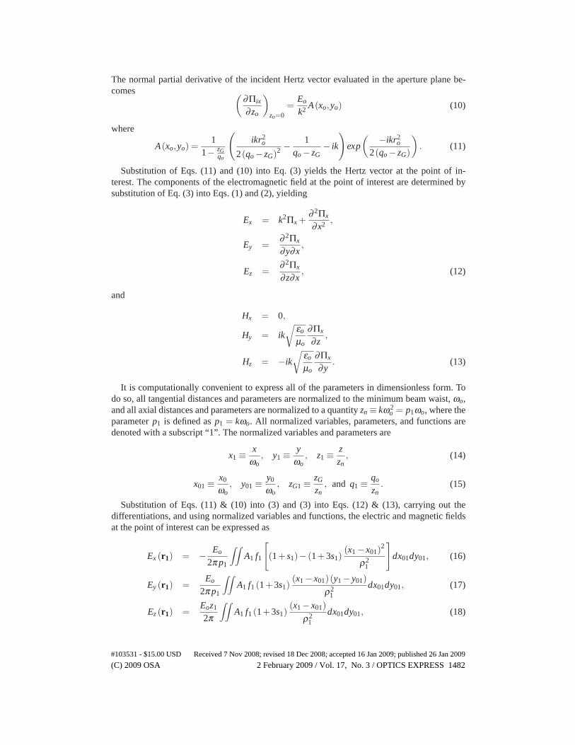
Figure 2 is a collection of calculations of the relative intensity of the light field for a = 4ωa
using the complete GHVDT outlined previously, and using the purely Gaussian Yariv model.The intensity calculated in the plots, Sz/So, is the normalized z-component of the Poynting vec-tor of the electromagnetic fields. All intensities of Fig.2 are normalized to the peak intensity inthe focal plane. Figures 2(a) and (b) are calculations where zG = 0, or the focal plane is coplanarwith the aperture plane. When the focal plane is coplanar with the aperture plane, calculationsfor the intensity versus radial position, Fig. 2(a), reproduce the unperturbed incident Gaussianbeam using the Yariv model in the aperture plane. Figure 2(b) shows that the calculated on-axis intensity for axial positions beyond the aperture plane using GHVDT also reproduce theexpected axial behavior for diverging TEM00 purely Gaussian beams.
Figures 2(c) and (d) are calculations for zG = 0.01 m, where the focal plane is located 1cm beyond the aperture plane. The incident Hertz vector (Eq. 9) in the aperture plane is onewhich yields a converging focused Gaussian beam with a width in the aperture plane whichfollows that of Eq. (27), or ωa = 99ωo, and the normalized peak intensity in the aperture planeis 1× 10⁻⁴. Using the full GHVDT and a zG value of 1 cm, Fig. 2(c) is a calculation of thenormalized intensity versus radial position for a distance of 1 cm beyond the aperture plane.Note that calculations using GHVDT for the regime of a � ωa reproduce calculated behaviorusing the Yariv model. For an unperturbed converging Gaussian beam, the on-axis intensityis expected to follow a Lorentzian function with an offset maximum occurring at the axiallocation of the focal plane, and having a normalized intensity of 1. Using GHVDT and inputparameters of zG = 0.01 m and a = 4ωa, the expected on-axis Gaussian behavior is reproduced,as illustrated in Fig. 2(d).
For the pure diffraction regime, the parameters chosen are zG = 0.01 m, and values of a/ωa <0.016. For these values of a/ωa, the variation between the intensity at the center of the apertureand the edge of the aperture is less than 0.05%. Thus the incident Hertz vector in the apertureregion is virtually uniform, and calculations using GHVDT should reproduce those for a planewave incident upon a circular aperture. Thus, the model chosen for comparison is that of Hertzvector diffraction theory, HVDT, applied to the diffraction of a plane wave incident upon a
(C) 2009 OSA 2 February 2009 / Vol. 17, No. 3 / OPTICS EXPRESS 1484#103531 - $15.00 USD Received 7 Nov 2008; revised 18 Dec 2008; accepted 16 Jan 2009; published 26 Jan 2009
1.0
0.8
0.6
0.4
0.2
0.0
Sz
/ So
0.01100.01050.01000.00950.0090
on axis position (meters)
(d) GHVDT Yariv
1.0
0.8
0.6
0.4
0.2
0.0
Sz
/ So
-2 -1 0 1 2x position (x / ωο)
(c) GHVDT Yariv
1.0
0.8
0.6
0.4
0.2
0.0
Sz
/ So
5004003002001000
on axis position (microns)
(b) GHVDT Yariv
1.0
0.8
0.6
0.4
0.2
0.0S
z / S
o-2 -1 0 1 2
x position (x / ωο)
(a) GHVDT Yariv
Fig. 2. Calculated Gaussian behavior for a/ωa = 4 using GHVDT. Figures (a) and (b)are the normalized intensity versus x in the aperture plane and versus z, respectively, forzG = 0. Figures (c) and (d) are the normalized intensity versus x in the focal plane andversus z, respectively, for zG = 0.01 m. Calculated intensity distributions using a purelyGaussian beam propagation model, Yariv, are included for comparison purposes.
(C) 2009 OSA 2 February 2009 / Vol. 17, No. 3 / OPTICS EXPRESS 1485#103531 - $15.00 USD Received 7 Nov 2008; revised 18 Dec 2008; accepted 16 Jan 2009; published 26 Jan 2009
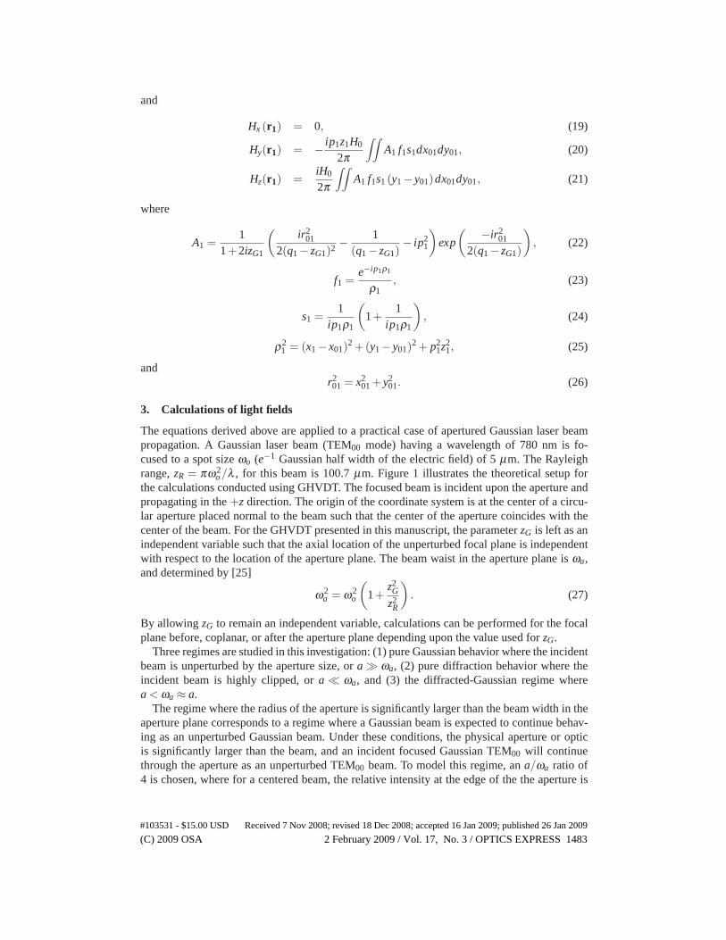
circular aperture [4]. For a complete description of HVDT applied to a plane wave incidentupon a circular aperture and comparisons of that model to other vector diffraction models seeref. [4]. An important parameter in the pure diffraction regime is the ratio of the aperture radiusto the wavelength of the light, a/λ . According to HVDT applied to plane wave diffraction,the on-axis intensity will oscillate as a function of increasing axial distance. The number ofoscillations of the on-axis intensity will be equal to the a/λ ratio [4]. The maximum on-axisintensity will have a value of 4 times the normalized incident intensity and will be locatedat a position of z = a2/λ . In the aperture plane, the central intensity will modulate about thenormalized incident intensity value as a function of the aperture to wavelength ratio due toscattering effects of the aperture edge [19]. Modulations in the fields within the aperture planewere both experimentally measured and calculated using HVDT by Bekefi in 1953 [19]. Theintensity value at the center of the aperture plane will be a maximum for integer values of thea/λ ratio, and will be a minimum for half integer values. Using HVDT, the z-component ofthe Poynting vector at the center of the aperture will have a normalized maximum value in theaperture plane of 1.5 and a minimum value of 0.5 [4].
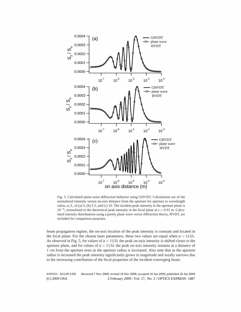
Figure 3 is a calculation of the normalized on-axis z-component of the Poynting vector usingGHVDT for a/λ ratios of (a) 5, (b) 5.5, and (c) 10, and an unperturbed focal plane location ofzG = 0.01 m. Note that the intensity is normalized to the expected peak Gaussian intensity inthe focal plane of an unperturbed beam, which makes the normalized intensity incident uponthe aperture 10−4. Figure 3 also includes plots for the calculated on-axis intensity distributionsaccording to HVDT of a plane wave incident upon a circular aperture. Note that all aspects ofthe calculations in Fig. 3 for a highly clipped, converging, focused Gaussian beam reproducethose expected for the diffraction of a plane wave even though the GHVDT still contains all ofthe phase information for a converging focused Gaussian TEM00 within input light field.
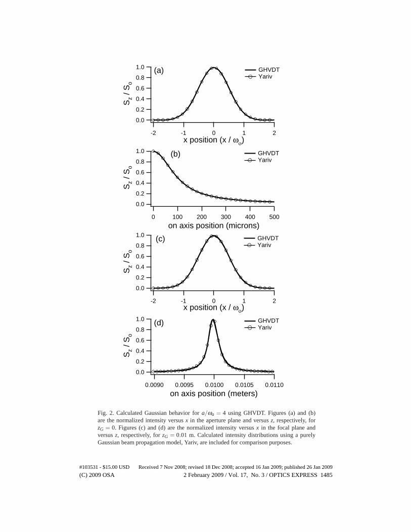
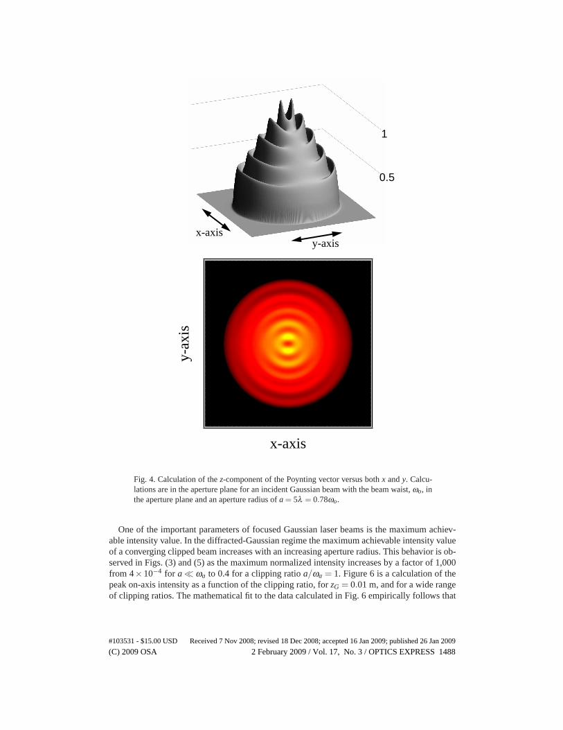
In the diffracted-Gaussian regime, the a/ωa ratio enters the region of ∼ 0.1 to ∼ 1, and thebehavior of the light field within and beyond the aperture plane is neither pure diffractive be-havior nor pure Gaussian behavior. This is a regime where traditional diffraction models andGaussian beam propagation models are invalid. To the best of the authors’ knowledge, no vectordiffraction theory exists in the literature for a focused diffracted-Gaussian beam. Thus, compar-ison of light field distributions for the model presented here to other vector diffraction modelsis currently not possible. An example of a calculation only possible with the GHVDT presentedhere is the normalized intensity illustrated in Fig. 4. Figure 4 is the z-component of the Poynt-ing vector as a function of both x and y in the aperture plane for the focal plane coplanar withthe aperture plane (zG = 0), an aperture radius of a = 5λ = 0.78ωo, and the polarization of theincident light along the x-axis. For an a/ωa ratio of 0.78, the intensity of the incident light onthe edge of the aperture is 29.6% of the value at the center of the aperture. The resulting lightdistribution is one of a partial Gaussian beam profile which is perturbed by the scattering effectsof the incident light field on the aperture itself. According to experimental measurements [19]and calculations using HVDT [4], the scattering modulations are strongest along the axis per-pendicular to the incident light polarization, and weakest along the axis parallel to the incidentlight polarization, and the number of oscillations from the center of the aperture to the apertureedge is equal to the a/λ ratio.
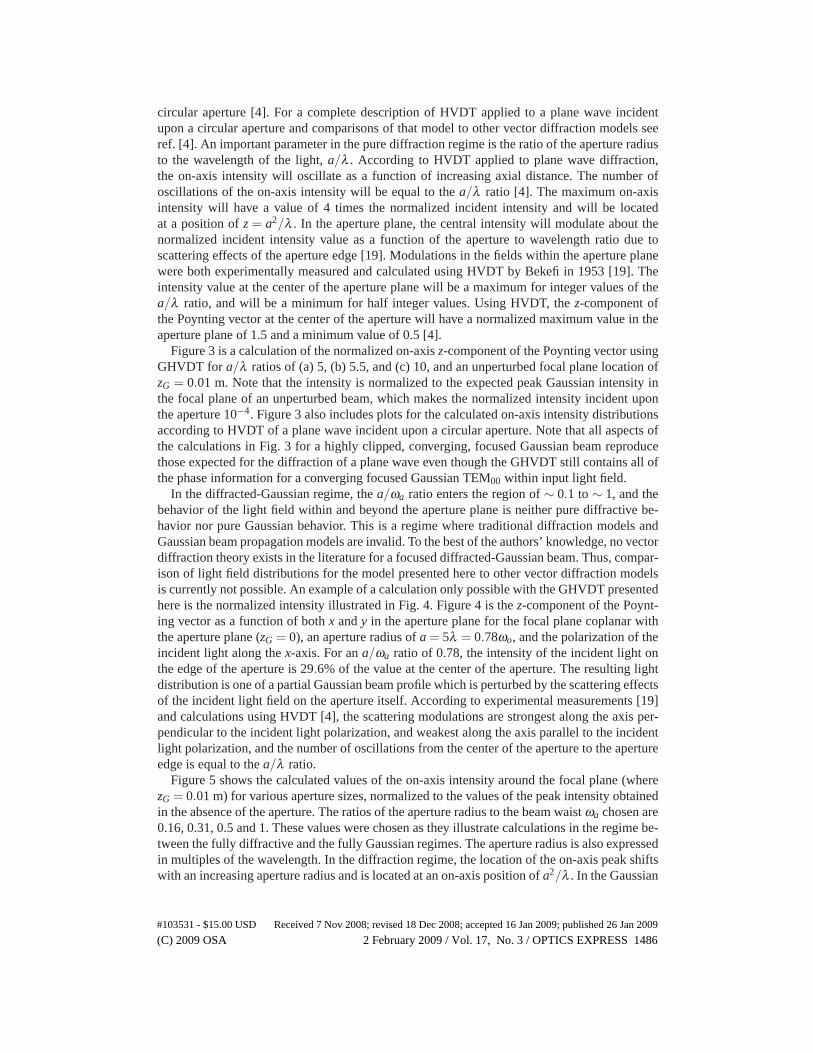
Figure 5 shows the calculated values of the on-axis intensity around the focal plane (wherezG = 0.01 m) for various aperture sizes, normalized to the values of the peak intensity obtainedin the absence of the aperture. The ratios of the aperture radius to the beam waist ωa chosen are0.16, 0.31, 0.5 and 1. These values were chosen as they illustrate calculations in the regime be-tween the fully diffractive and the fully Gaussian regimes. The aperture radius is also expressedin multiples of the wavelength. In the diffraction regime, the location of the on-axis peak shiftswith an increasing aperture radius and is located at an on-axis position of a2/λ . In the Gaussian
(C) 2009 OSA 2 February 2009 / Vol. 17, No. 3 / OPTICS EXPRESS 1486#103531 - $15.00 USD Received 7 Nov 2008; revised 18 Dec 2008; accepted 16 Jan 2009; published 26 Jan 2009
0.0004
0.0003
0.0002
0.0001
0.0000
Sz
/ So
10-7
10-6
10-5
10-4
10-3
on axis distance (m)
(c) GHVDT plane wave
HVDT
0.0004
0.0003
0.0002
0.0001
0.0000S
z / S
o
10-7
10-6
10-5
10-4
10-3
(a) GHVDT plane wave
HVDT
0.0004
0.0003
0.0002
0.0001
0.0000
Sz
/ So
10-7
10-6
10-5
10-4
10-3
(b) GHVDT plane wave
HVDT
Fig. 3. Calculated plane-wave diffraction behavior using GHVDT. Calculations are of thenormalized intensity versus on-axis distance from the aperture for aperture to wavelengthratios, a/λ , of (a) 5, (b) 5.5, and (c) 10. The incident peak intensity in the aperture plane is10−4, normalized to the theoretical peak intensity in the focal plane at z = 0.01 m. Calcu-lated intensity distributions using a purely plane wave vector diffraction theory, HVDT, areincluded for comparison purposes.
beam propagation regime, the on-axis location of the peak intensity is constant and located inthe focal plane. For the chosen laser parameters, these two values are equal when a = 113λ .As observed in Fig. 5, for values of a < 113λ the peak on-axis intensity is shifted closer to theaperture plane, and for values of a > 113λ the peak on-axis intensity remains at a distance of1 cm from the aperture even as the aperture radius is increased. Also note that as the apertureradius is increased the peak intensity significantly grows in magnitude and axially narrows dueto the increasing contribution of the focal properties of the incident converging beam.
(C) 2009 OSA 2 February 2009 / Vol. 17, No. 3 / OPTICS EXPRESS 1487#103531 - $15.00 USD Received 7 Nov 2008; revised 18 Dec 2008; accepted 16 Jan 2009; published 26 Jan 2009
y-ax
is
x-axis
y-axisx-axis
0.5
1
Fig. 4. Calculation of the z-component of the Poynting vector versus both x and y. Calcu-lations are in the aperture plane for an incident Gaussian beam with the beam waist, ωo, inthe aperture plane and an aperture radius of a = 5λ = 0.78ωo.
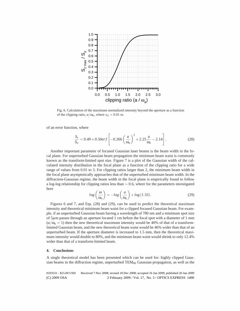
One of the important parameters of focused Gaussian laser beams is the maximum achiev-able intensity value. In the diffracted-Gaussian regime the maximum achievable intensity valueof a converging clipped beam increases with an increasing aperture radius. This behavior is ob-served in Figs. (3) and (5) as the maximum normalized intensity increases by a factor of 1,000from 4×10⁻⁴ for a � ωa to 0.4 for a clipping ratio a/ωa = 1. Figure 6 is a calculation of thepeak on-axis intensity as a function of the clipping ratio, for zG = 0.01 m, and for a wide rangeof clipping ratios. The mathematical fit to the data calculated in Fig. 6 empirically follows that
(C) 2009 OSA 2 February 2009 / Vol. 17, No. 3 / OPTICS EXPRESS 1488#103531 - $15.00 USD Received 7 Nov 2008; revised 18 Dec 2008; accepted 16 Jan 2009; published 26 Jan 2009
0.4
0.3
0.2
0.1
0.0
Sz
/ So
0.0012 3 4 5 6
0.012 3 4 5 6
0.1on axis distance (m)
(d)
0.05
0.04
0.03
0.02
0.01
0.00
Sz
/ So
0.0012 3 4 5 6
0.012 3 4 5 6
0.1
(c)
0.008
0.006
0.004
0.002
0.000
Sz
/ So
0.0012 3 4 5 6
0.012 3 4 5 6
0.1
(b) GHVDT plane wave
HVDT
0.0012
0.0008
0.0004
0.0000S
z / S
o
0.0012 3 4 5 6
0.012 3 4 5 6
0.1
(a) GHVDT plane wave
HVDT
Fig. 5. Calculations of the normalized on-axis intensity for the regime between purediffractive and pure Gaussian behavior for zG = 0.01 m and (a) a = 100λ = 0.16ωa, (b)a = 200λ = 0.31ωa, (c) a = 318λ = 0.5ωa, and (d) a = 636λ = ωa. All intensities are nor-malized to the peak unperturbed focal spot intensity. Calculated intensity distributions us-ing a purely plane wave vector diffraction theory, HVDT, are included to illustrate the tran-sition of the GHVDT model from the diffraction regime to the focused diffracted-Gaussianregime.
(C) 2009 OSA 2 February 2009 / Vol. 17, No. 3 / OPTICS EXPRESS 1489#103531 - $15.00 USD Received 7 Nov 2008; revised 18 Dec 2008; accepted 16 Jan 2009; published 26 Jan 2009
1.0
0.9
0.8
0.7
0.6
0.5
0.4
0.3
0.2
0.1
0.0S
z m
ax /
So
3.02.52.01.51.00.50.0
clipping ratio (a / ωa)
Fig. 6. Calculation of the maximum normalized intensity beyond the aperture as a functionof the clipping ratio, a/ωa, where zG = 0.01 m.
of an error function, where
Sz
So= 0.49+0.50er f
[−0.266
(a
ωa
)2
+2.25a
ωa−2.14
]. (28)
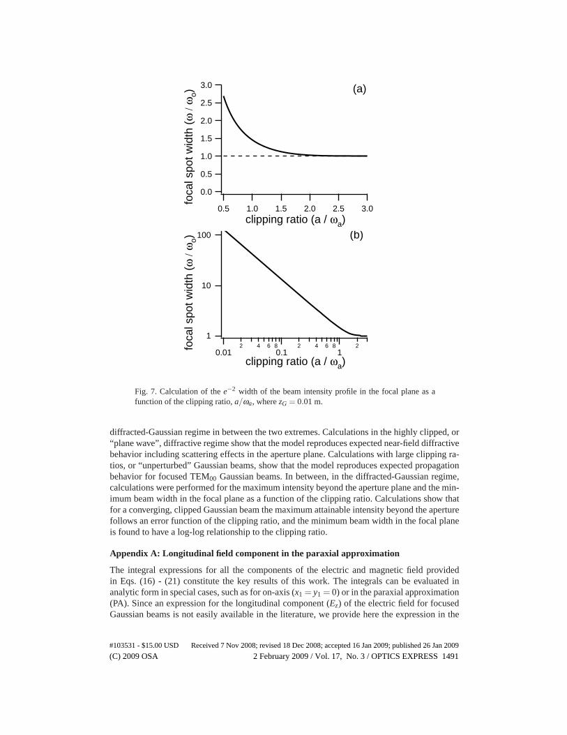
Another important parameter of focused Gaussian laser beams is the beam width in the fo-cal plane. For unperturbed Gaussian beam propagation the minimum beam waist is commonlyknown as the transform-limited spot size. Figure 7 is a plot of the Gaussian width of the cal-culated intensity distribution in the focal plane as a function of the clipping ratio for a widerange of values from 0.01 to 3. For clipping ratios larger than 2, the minimum beam width inthe focal plane asymptotically approaches that of the unperturbed minimum beam width. In thediffraction-Gaussian regime, the beam width in the focal plane is empirically found to followa log-log relationship for clipping ratios less than ∼ 0.6, where for the parameters investigatedhere
log
(ωωo
)= −log
(a
ωa
)+ log(1.33) . (29)
Figures 6 and 7, and Eqs. (28) and (29), can be used to predict the theoretical maximumintensity and theoretical minimum beam waist for a clipped focused Gaussian beam. For exam-ple, if an unperturbed Gaussian beam having a wavelength of 780 nm and a minimum spot sizeof 5μm passes through an aperture located 1 cm before the focal spot with a diameter of 1 mm(a/ωa = 1) then the new theoretical maximum intensity would be 40% of that of a transform-limited Gaussian beam, and the new theoretical beam waist would be 46% wider than that of anunperturbed beam. If the aperture diameter is increased to 1.5 mm, then the theoretical maxi-mum intensity would double to 80%, and the minimum beam waist would shrink to only 12.4%wider than that of a transform-limited beam.
4. Conclusions
A single theoretical model has been presented which can be used for: highly clipped Gaus-sian beams in the diffraction regime, unperturbed TEM00 Gaussian propagation, as well as the
(C) 2009 OSA 2 February 2009 / Vol. 17, No. 3 / OPTICS EXPRESS 1490#103531 - $15.00 USD Received 7 Nov 2008; revised 18 Dec 2008; accepted 16 Jan 2009; published 26 Jan 2009
1
10
100
foca
l spo
t wid
th (
ω /
ωo)
0.012 4 6 8
0.12 4 6 8
12
clipping ratio (a / ωa)
(b)
3.0
2.5
2.0
1.5
1.0
0.5
0.0fo
cal s
pot w
idth
(ω
/ ω
o)
3.02.52.01.51.00.5clipping ratio (a / ωa)
(a)
Fig. 7. Calculation of the e−2 width of the beam intensity profile in the focal plane as afunction of the clipping ratio, a/ωa, where zG = 0.01 m.
diffracted-Gaussian regime in between the two extremes. Calculations in the highly clipped, or“plane wave”, diffractive regime show that the model reproduces expected near-field diffractivebehavior including scattering effects in the aperture plane. Calculations with large clipping ra-tios, or “unperturbed” Gaussian beams, show that the model reproduces expected propagationbehavior for focused TEM00 Gaussian beams. In between, in the diffracted-Gaussian regime,calculations were performed for the maximum intensity beyond the aperture plane and the min-imum beam width in the focal plane as a function of the clipping ratio. Calculations show thatfor a converging, clipped Gaussian beam the maximum attainable intensity beyond the aperturefollows an error function of the clipping ratio, and the minimum beam width in the focal planeis found to have a log-log relationship to the clipping ratio.
Appendix A: Longitudinal field component in the paraxial approximation
The integral expressions for all the components of the electric and magnetic field providedin Eqs. (16) - (21) constitute the key results of this work. The integrals can be evaluated inanalytic form in special cases, such as for on-axis (x1 = y1 = 0) or in the paraxial approximation(PA). Since an expression for the longitudinal component (Ez) of the electric field for focusedGaussian beams is not easily available in the literature, we provide here the expression in the
(C) 2009 OSA 2 February 2009 / Vol. 17, No. 3 / OPTICS EXPRESS 1491#103531 - $15.00 USD Received 7 Nov 2008; revised 18 Dec 2008; accepted 16 Jan 2009; published 26 Jan 2009
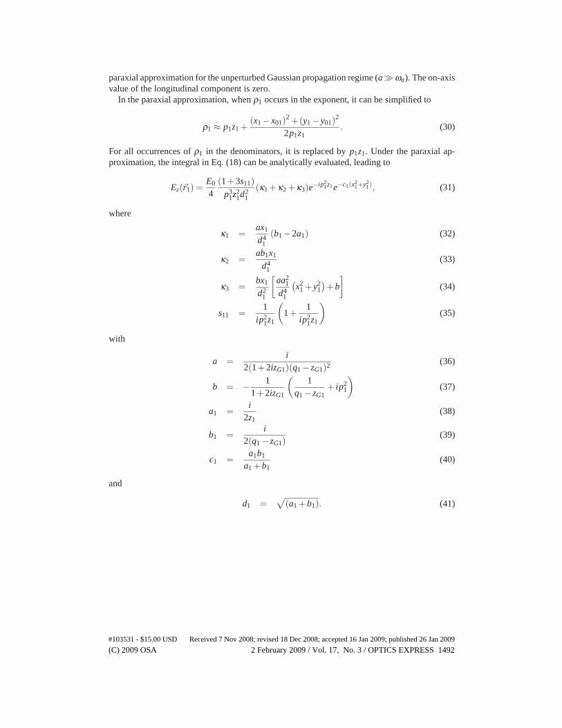
paraxial approximation for the unperturbed Gaussian propagation regime (a�ωa). The on-axisvalue of the longitudinal component is zero.
In the paraxial approximation, when ρ1 occurs in the exponent, it can be simplified to
ρ1 ≈ p1z1 +(x1 − x01)
2 +(y1 − y01)2
2p1z1. (30)
For all occurrences of ρ1 in the denominators, it is replaced by p1z1. Under the paraxial ap-proximation, the integral in Eq. (18) can be analytically evaluated, leading to
Ez(�r1) =E0
4(1+3s11)
p31z2
1d21
(κ1 +κ2 +κ3)e−ip21z1e−c1(x2
1+y21), (31)
where
κ1 =ax1
d41
(b1 −2a1) (32)
κ2 =ab1x1
d41
(33)
κ3 =bx1
d21
[aa2
1
d41
(x2
1 + y21
)+b
](34)
s11 =1
ip21z1
(1+
1
ip21z1
)(35)
with
a =i
2(1+2izG1)(q1 − zG1)2 (36)
b = − 11+2izG1
(1
q1 − zG1+ ip2
1
)(37)
a1 =i
2z1(38)
b1 =i
2(q1 − zG1)(39)
c1 =a1b1
a1 +b1(40)
and
d1 =√
(a1 +b1). (41)
(C) 2009 OSA 2 February 2009 / Vol. 17, No. 3 / OPTICS EXPRESS 1492#103531 - $15.00 USD Received 7 Nov 2008; revised 18 Dec 2008; accepted 16 Jan 2009; published 26 Jan 2009