+ All Categories
Home > Documents > APPLICATION OF NEURAL NETWORK CONTROL

APPLICATION OF NEURAL NETWORK CONTROL

Date post: 12-Jan-2022
Category:
Upload: others
View: 2 times
Download: 0 times
Share this document with a friend
218
APPLICATION OF NEURAL NETWORK CONTROL TO DISTILLATION by PRIYABRATA DUTTA, B.Tech., M.Tech. A DISSERTATION IN CHEMICAL ENGINEERING Submitted to the Graduate Faculty of Texas Tech University in Partial Fulfillment of the Requirements for the Degree of DOCTOR OF PHILOSOPHY Approved
Transcript

APPLICATION OF NEURAL NETWORK CONTROL

TO DISTILLATION

by

PRIYABRATA DUTTA, B.Tech., M.Tech.

A DISSERTATION

IN

CHEMICAL ENGINEERING

Submitted to the Graduate Faculty of Texas Tech University in

Partial Fulfillment of the Requirements for

the Degree of

DOCTOR OF PHILOSOPHY

Approved

ACKNOWLEDGMENTS

I wish to take this opportunity to convey my sincere thanks to my research

advisor, Dr. Russell Rhinehart. His encouragement, suggestions and guidance in many

matters have greatly helped me in achieving my academic goals. What I like most is his

unique way of teaching, way of providing hints and making us understand the problem and

the direction of solution in a lucid and transparent manner. I acknowledge him for being

with me throughout my research. His friendly yet professional attitude towards students

has made him a 'superb professor' in my eyes. I feel privileged to get an opportunity to

work with an advisor like 'Russ\

I am thankful to Dr. James B. Riggs for giving me admission to Texas Tech and

providing me an opportunity to work in my desired field. I would also like to give my

special thanks to Dr. Brian Oldham for opening a door to the Computer Science

Department. His calm disposition and brief and to the point answer to all my questions

have always been an extra encouragement to me. This dissertation would not have been

complete without the corrections by Dr. Robert Bethea. I appreciate his time, effort and

interest in the preparation of this dissertation. I also wish to convey my thanks to Dr. Hua

Li for his advice, questions and comments as my committee member. Thanks are also

extended to the members of the Process Control and Optimization Consortium at Texas

Tech University for financial support of this work. Although, I did not get much

opportunity to take many chemical engineering courses with the professors in this

department, I never felt out of place at any time. For this, my sincere thanks go to Dr.

Narayan, Dr. Tock, Dr. Mann, Dr. Heichelheim and Dr. Wiesner.

ii

I acknowledge Mr. Robert Spruill for extending his helping hand during the phase

of 'instrumental trouble' of the experimental setup. Tammy and Mary, the two pillars of

administration, will always be remembered by me as the best two persons in the Chemical

Engineering Department. Thanks are also due to Sandeep Lai, Siva, Ramesh, Mahesh,

Ganesh, Abe, Bala, Scott and Joe for their friendship during my stay at Tech.

My last one and a half year stay at Lubbock would not be any better without the

assistance of my lovely wife 'Adity'. Besides her moral support and encouragement, her

delicious cooking kept me 'going and going' during the last phase of the long

experimental runs. Finally, I would like to say that it would not be possible for me to

pursue my graduate studies in the US without the support of my mom, my brothers and

sisters across the ocean.

in

TABLE OF CONTENTS

ACKNOWLEDGEMENTS ii ABSTRACT vi LIST OF TABLES viii LIST OF FIGURES ix NOMENCLATURE xii

CHAPTER I INTRODUCTION 1

II LITERATURE SURVEY 7 2.1 Distillation Control 7

2.1.1 Importance 7 2.1.2 Objectives 7 2.1.3 Constraints 8 2.1.4 Distillation Control Literature 8

2.2 Literature on Linear and Nonlinear Control 13 2.2.1 Linear Model Based Control 13 2.2.2 Nonlinear Model Based Control 15

2.3 Neural Network Control 17 2.3.1 Importance of Neural Networks in Control 17 2.3.2 Literature on Neural Network Control 18 2.3.3 An Introduction to Neural Networks 19 2.3.4 Training of Neural Networks 19

2.3.4.1 Backpropagation 23 2.3.4.2 Optimization Approach 25

2.4 Self-Tuning Filter 28

IH EXPERIMENTAL SETUP AND SIMULATOR 3 2

3.1 Experimental Setup 32 3.1.1 Distillation Unit 32 3.1.2 Instrumentation 35 3.1.3 Data Acquisition and Control System 38

3.1.4 Interfacing Program Development 38 3.1.5 Control Difficulties 40

3.2 Simulator 42 3.2.1 Model Equations 42 3.2.2 Assumptions 44 3.2.3 Design and Operating Conditions 45

IV CONTROLLER DEVELOPMENT 4 8

4.1 Neural Network Model Inverse and State Prediction 43

IV

4 2 Neural Network Model and Gain Prediction <-,-4.3 Optimization and Constraint Handling (HRO) 6 ,

V CONTROL RESULTS 6 5

5.1 Simulator Results , , 5.1.1 Distillation Control with NN Gain Prediction 6 7

5.1.2 Distillation Control with Gain Prediction (Constrained Control Mode) 72

5.2 Experimental Results 7^ 5.2.1 NN Control in State Inverse Mode on SISO systems

(Heaters) 7^ 5.2.2 NN Control in State Inverse Mode on Distillation

Column go 5.2.2.1 Setpoint Tracking Q2

5.2.2.2 Disturbance Rejection Qo 5.2.3 NN Control of Distillation Column in Gain Prediction

Mode 1 0 4

5.2.3.1 Setpoint Tracking 1 0 9

5.2.3.2 Disturbance Rejection 120 5.2.4 Constrained Control of Distillation Column with NN

Gain Prediction 129 5.2.5 Process Model Mismatch ,^^ 5.2.6 ATV Results 1 3 g

VI COMPARISON OF CONTROL RESULTS 1 4 7

6.1 Performance Comparison 1 4 7

6.2 Other Issues 1 5 3

VII CONCLUSION AND RECOMMENDATION 1 5 7

7.1 Conclusions , 5 7

7.2 Recommendations , 5 g

REFERENCES 1 6 0

APPENDICES A. PMBC.ACC and [DMC]™ CONTROL RESULTS 1 6 6

B. INSTRUMENT CALIBRATION AND PROPERTY CORRELATION 194

C. SOFTWARE 206

ABSTRACT

Distillation control is challenging due to its coupled, nonlinear, nonstationary, and

slow dynamic behavior. Like distillation columns, most chemical processes are usually

nonlinear and nonstationary. This nonlinearity greatly limits the effectiveness of linear

controllers, especially when the process is operated away from the nominal operating

region. Nonlinear controllers, based on phenomenological models, can be developed.

However, it is still a very difficult task in real practice, in terms of computational power,

to implement these controllers on-line, because the entire model needs to be solved within

each control interval. Neural networks give us an alternative approach to model a

nonlinear process, and a controller based on this model can overcome the issues of on-line

computational problems. Besides nonlinearity, many practical control problems possess

constraints on the input, state, and output variables. The ability to handle constraints is

essential for any algorithm to be implemented on real processes. Thus strategies for

constraint handling within model-based controllers have become one of the more popular

research topics.

In this dissertation, a constrained optimization technique for control which uses a

neural network gain prediction approach has been developed and implemented on a

laboratory distillation column as well as on a dynamic simulator. Here, the neural

networks are trained based on a phenomenological model. Also, experimental results have

been obtained to confirm the applicability of a neural network model-based controller

using an inverse of a state-prediction approach that was developed and simulated earlier

VI

by Ramchandran and Rhinehart (1994). In addition, two separate single-input-single-

output (SISO) controllers using the inverse of the state-prediction approach are

implemented on the feed and reflux preheaters of the column.

vu

LIST OF TABLES

3.1 Relative Gain Array 40

5.1 Tests on Simulator (Servo Mode) 67

5.2 Tests on Simulator (Regulatory Mode) 70

5.3 Comparative Study on Feed Preheater Control g5

5.4 Synopsis of experimental runs in control performance study 93

5.5 Setpoint tracking with neural network control in inverse of the state prediction mode (Case 1) 94

5.6 Disturbance rejection with neural network control in inverse of the state prediction mode (Case 2) IOQ

5.7 Disturbance rejection with neural network control in inverse of the state prediction mode (Case 3) 104

5.8 Setpoint tracking with neural network control in gain prediction mode(Case 1) H4

5.9 Disturbance rejection with neural network control in gain prediction mode (Case 2) 12i

5.10 Disturbance rejection with neural network control in gain prediction

mode (Case 3) 125

5.11 Material Balance Closure in Experiments 134

6.1 Quantitative Comparison of Controller Performance 148

6.2 Summary of Control Performance 154

Vl l l

LIST OF FIGURES

2.1 Feedforward neural network architecture (4-5-1) 20

2.2 Signal processing within a neuron 21

3.1 Schematic flow diagram of the setup 33

3.2 Instrumentation and DAC system 36

4.1 Neural network model-based control strategy in inverse of a state

prediction approach 52

4.2 Neural network model-based control strategy with gain prediction 50

5.1 Setpoint tracking with neural network gain prediction approach on simulator 68

5.2 Disturbance rejection with NN gain prediction approach on the distillation column simulator , 71

5.3 Constrained control on simulator with NN gain prediction using setpoint changes 73

5.4 Constrained control on simulator with NN gain prediction using feed composition disturbance 74

5.5 Steady-state temperature profile of feed preheater 78

5.6 Training result on manipulated variable of feed preheater 79

5.7 PI control of feed preheater g0

5.8 Internal Model control of feed preheater 4 g2

5.9 Model predictive control of feed preheater g3

5.10 Neural network control of feed preheater g4

5.11 Training result on manipulated variable of reflux preheater g7

5.12 Neural network control on reflux preheater gg

IX

5.13 Training result on manipulated variables in inverse of state prediction mode 90

5.14 Setpoint tracking with neural network control in inverse of state prediction mode (Case 1) 95

5.15 Disturbance rejection with neural network control in inverse of state prediction mode (Case 2) 101

5.16 Disturbance rejection with neural network control in inverse of state

prediction mode (Case 3) 106

5.17 Training results on gains in gain prediction approach U0

5.18 Setpoint tracking with neural network control in gain prediction mode (Casel) n 5

5.19 Disturbance rejection with neural network control in gain prediction mode (Case 2) 122

5.20 Disturbance rejection with neural network control in gain prediction mode (Case 3) 126

5.21 Constrained control with neural network gain prediction using feed

composition disturbance 130

5.22 Process Model Mismatch 236

5.23 Autotune Variation Relay Feedback I^o

5.24 PI Control with ATV (Tyerus-Luyben with DTF=3.0) 1 4 3

5.25 PI Control with ATV (Ziegler-Nichols with DTF=4.5) 1 4 5

A.1 PMBC Controller Casel 1 6 7

A.2 PMBC Controller Case 2 1 7 0

A.3 PMBC Controller Case 3 1 7 3

A.4 [DMC]™ Controller Case 1 1 7 6

A.5 [DMC]™ Controller Case 2 179

A.6 [DMC]™ Controller Case 3 182

A.7 ACC Controller Casel 185

A.8 ACC Controller Case2 188

A.9 ACC Controller Case3 191

B.l Reboiler Power Characteristic 195

B.2 Reverse Power Relationship 197

B.3 Reflux Pump Calibration 198

B.4 Feed Pump Calibration 200

B.5 Refractive Index versus Liquid Composition for Methanol-Water

Mixture 201

B.6 Distillate Flowrate Calibration 203

B.7 Bottom Flowrate Calibration 204 B.8 Screen Setup 205

XI

NOMENCLATURE

[DMC]™

GMC

HRO

IDCOM

IMC

MAC

MEMO

MPC

NMPC

NN

PMBC

RGA

SISO

VLE

Dynamic Matrix Control (with trademark)

Generic Model Control

Heuristic Random Optimization

IDentification and COMmand

Internal Model Control

Model Algorithmic Control

Multi-Input-Multi-Output

Model Predictive Control

Nonlinear Model Predictive Control

Neural Network

Process Model-Based Control

Relative Gain Array

Single-Input-Single-Output

Vapor-Liquid Equilibria

xn

CHAPTER I

INTRODUCTION

The increasing stress on 'quality' in process operation and economic performance

is placing significant demands on existing control methodologies. One potential means by

which to achieve enhanced process control performance is to adopt a model-based

strategy. Algorithms which have attracted particular interest are based on the long-range

prediction of process outputs commonly known as model predictive control (MPC)

(Cutler et al., 1979; Mehra et al., 1985). MPC algorithms have been recognized as

effective tools for handling some of the most difficult control problems in industry. MPC

has been implemented successfully in several chemical industries in the US (Exxon, TX,

Hokanson et al., 1989; Sun Refining, OH, Trans et al., 1989) and in other countries

(Sarnia Refinery, Ontario, Canada, Cutler et al., 1987; Pembroke Cracking Company, UK,

Park, 1988). MPC schemes derive some of their industrial appeal from their ability to

handle input and output constraints, time delays, non-minimum phase behavior and

multivariable systems.

Two popular variations of the MPC algorithms are dynamic matrix control

[DMC]™(Cutler et al., 1979, 1987) and model algorithmic control [MAC] (Mehra et al.,

1985). The underlying strategy of the MPC algorithms is to use a model to predict the

future output trajectory of the process and then to compute a controller action to minimize

the difference between the predicted trajectory and a user-specified trajectory.

Despite the commercial success enjoyed by MPC in some industries, there has not

been an overwhelming acceptance in general. Whilst a number of reasons for this can be

highlighted, one of the main problems is the failure to satisfy robustness, i.e., maintaining

control performance without degradation at different operating regions and with changing

process conditions. Two of the principal causes of poor robustness are inability to obtain a

correct process model and designing a controller structure that is insensitive to

process/model mismatch. The process model structure most often assumed is a linear time

series. The linear approximation approach can be useful under nominal operating

conditions to which the controller is tuned. However, the tuning often shows poor

performance under transient upsets in which the process "moves" into another operating

region where the original linear model is not a good representation of the process. Under

this situation, a globally accurate model proves to be most useful. One possibility is to

allow the linear model to adapt to process changes; but, in real process environments, the

computational demands placed upon adaptive schemes by everyday process occurrences

such as flow, composition, and thermal disturbances can be significant. Furthermore,

'jacketing' code to protect the algorithms from these upsets can be developed, but the

difficulty in taking into account all likely occurrences should not be underestimated. In

general, the greater the reliance which is placed upon adaptation, the higher is the

likelihood of problems. If the reliance upon adaptation is to be avoided, whilst still

maintaining a low level of process/model mismatch, then a model which is more capable of

describing nonlinearities should be utilized.

Several workers have investigated the use of a nonlinear process representation

within a model-based control strategy. Lee and Sullivan (1988) demonstrated the utility of

the technique in an application to a forced-circulation single-stage evaporator which is a

nonlinear interacting process. Their Generic Model Control (GMC) strategy bears strong

similarities to the Nonlinear Internal Model Control (NIMC) approach exhorted by Garcia

and Morari (1982) and Economou and Morari (1986). The NIMC method made use of a

Newton-type algorithm to provide a tractable solution of the nonlinear model. Recently,

Ganguli and Saraf (1993) applied an improved nonlinear model predictive control

(NMPC) (Eaton and Rawlings, 1990) to control a distillation column start-up. Due to the

need for solving an on-line optimization problem, the computational demand of the control

procedure proposed by Ganguli and Saraf (1993) is very high.

Whilst nonlinear system models can provide good process performance, realistic

system models are often very difficult and time consuming to derive, and they may be

impossible to specify, especially when the basic mechanisms of a process are not

completely understood. A desirable objective would therefore be to develop a technique

which possesses generality of model structure (facilitating rapid and cheap development),

which could also be capable of learning and expressing the process nonlinearities and

complexities, and which computes rapidly. One such approach that has recently become

popular is the use of artificial neural networks (ANN), or simply neural network (NN)

(Bhat and McAvoy, 1990; Bhagat, 1990; Thibault and Grandjean, 1992; MacMurray and

Himmelblau, 1993). Though this term, "neural network," originally came from the idea to

mimic human neuron activity, it is exclusively used in the scientific and engineering

community to represent a mathematical model for a real system correlating certain input

and output data spaces.

The most attractive property of a NN is its ability to represent any arbitrary

nonlinear functional mapping between the input and output data. This mapping is achieved

through a "training" process that takes place by repeatedly "showing" the input data and

the corresponding target outcomes to the net. During the "training" process, an optimizer

(or other techniques like back propagation) updates the values of NN weights (starting

with random small initial guesses) to minimize the sum of squared (model-predicted minus

data) errors. After a sufficient number of training iterations, the optimizer creates an

internal approximate process model (i.e., the NN architecture with calculated weights and

selected nodal functions) which can correlate the mapping between the desired output and

the corresponding inputs.

It is important to note that the NN internal model is not based on any specification

of the actual process mechanism; the optimizer generates this approximate model based on

the data set given to it. Due to the complete dependence of the neural networks on the

data sets, it is usually said that neural networks do not require any a priori fundamental

understanding of the investigated process. In reality, the above statement is not entirely

true. The control engineer has to have some process knowledge for effective

implementation of NN model-based controllers. Indeed, the critical point in developing a

robust NN model is selecting the most representative process input-output data sets, and

this selection can only be achieved through an understanding of the underlying process

phenomena.

It is often suggested that these neural network models may be easily obtained from

historical plant data, thus solving the problems associated with generating nonlinear

process models. But, in reality, gathering enough reliable informative sets of plant data,

over a wide enough operating region, for neural network training, is a formidable task.

Rather, a phenomenological model can be developed, and the data can often easily be

generated using this model for neural network training. In this study, a process simulator

of a distillation column is used to generate many sets of steady-state data at different

operating conditions. A neural network model is generated off-line based on these steady-

state data and subsequently applied to control a laboratory distillation column separating

a binary mixture of methanol and water in a dual-composition control mode.

Following successful implementation of steady-state model-based control by the

previous researchers at Texas Tech (Pandit, 1991; Gupta, 1994; Ramchandran, 1994), a

steady-state modeling approach is taken here. While dynamic models are 'right', steady-

state models are often used in process control because they are simple, compute rapidly,

and are easy to implement. While both tools have a place, the use of steady-state models,

coupled with experience and a general knowledge of distillation-column dynamics, is

adequate for many problems and often is more efficient than using dynamic models.

Steady-state modeling packages are available commercially from a number of vendors.

The models are easily manipulated and provide robust solutions. To make a change to the

solution conditions, only a few changes need to be made to the model input data. The

input data then are used by the software to find a new solution. Generally, very little time

is spent getting converged solutions, which allows us to efficiently generate the large

number of data necessary for the neural network training. One obvious limitation of

steady-state modeling, though, is that it tells nothing about the dynamic response, making

it difficult to apply to a dynamically ill-behaved system.

The major commercial advanced control approach, MPC, successfully handles

constraints and dynamics, but cannot handle nonlinear/nonstationary behavior. There are

three major problems for chemical process control: nonlinear/nonstationary behavior,

constraints, and ill-behaved dynamics. Often, nonlinearity and constraints are two major

problems in many chemical processes where the dynamics are well behaved. In our study,

the constraints are implemented on the manipulated variables based on a computationally

efficient optimization algorithm, Heuristic Random Optimization (HRO, Li and Rhinehart,

1996). This method along with the neural-network-modeling approach allowed

implementation of this controller with a small control interval (1/2 minute compared to 3

minutes in PMBC and DMC) (Pandit, 1991; Gupta, 1994). In many cases, a small control

interval offers better control performance. Accordingly, this controller handles the 2-

problem combination of nonlinearity and constraints that is very common in control

practice.

In summary, MPC handles constraints and ill-behaved dynamics but does not

consider the nonlinearity of the process. NMPC requires an extensive computational

approach and is still in the stage of theoretical development. Whereas, the controller in this

research study based on neural network modeling approach with HRO algorithm, though

does not qualify for "ill-behaved dynamics" (e.g., inverse response), takes care of the

common control problems of nonlinearities and steady-state constraints.

CHAPTER II

LITERATURE SURVEY

2.1 Distillation Control

2.1.1 Importance

Distillation control has a major impact upon the refining and chemical industries

due to its effect upon product uniformity, process throughput, and utility usage. Utility

usage for distillation in the US amounts to 3% of the annual US energy consumption. A

DOE report (Humphrey et al., 1991) estimated that improved distillation control would

reduce the energy consumption for distillation by 15% resulting in an energy savings of

360 trillion BTU/yr (equivalent to $1.6 billion/yr). Moreover, the economic savings

associated with improved distillation control for utility savings are, in general, small

compared with the value of improved uniformity and increased throughput.

2.1.2 Objectives

Two main facets of distillation controls are

• Product quality control

• Satisfaction of constraints.

The control system for a binary distillation in most cases must maintain the

concentration of one component in either the overhead or bottoms at a specified value

and maintain the composition at the other end of the column as close as possible to a

desired composition. This two-point composition control strategy must function

satisfactorily in the face of possible disturbances in (a) feed flowrate, (b) feed

composition, (c) feed temperature, (d) steam supply pressure, (e) condenser water supply

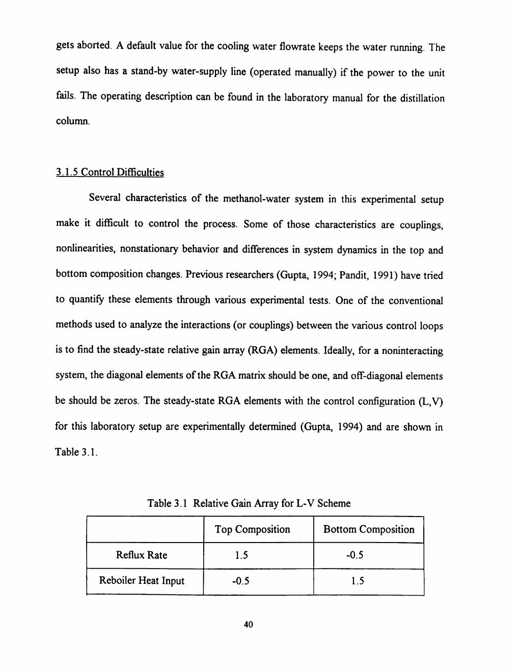
temperature, (f) ambient temperature (such as that caused by rainstorms), etc.

2.1.3 Constraints

For safe, satisfactory operation of the column, certain constraints must be

observed. For example:

• The column should not flood.

• Column pressure drop should be high enough to maintain effective column operation,

that is, to prevent serious weeping or dumping.

• The temperature difference in the reboiler should not exceed the critical temperature

difference.

• Column feed rate should not be so high as to overload reboiler or condenser heat-

transfer capacity.

• Boilup should not be so high that an increase will cause a decrease in product purity at

the top of the column.

• Column pressure should not exceed either a maximum or minimum permissible value.

2.1.4 Distillation Control Literature

The process control literature on distillation column control is vast; and there are

so many different types of control methods, algorithms, and control philosophies that it is

unrealistic to acknowledge all of them here. This section will limit the discussion strictly to

only those references related with this work.

8

Distillation column control is primarily a multivariate problem. A multi-input-

multi-output (MIMO) control can be decomposed into several single-input-single-output

(SISO) loops, and in the case of a binary distillation column, four variables, two products,

reflux drum level, and reboiler level are controlled using reflux flow, vapor boilup and two

product flows. The decomposition into four SISO loops can be made in many ways, giving

rise to different control structures.

Morari et al. (1987) provide guidelines for control configuration selection for

distillation columns. The paper suggested that the ratio configurations (e.g.,

reflux/distillate product and boilup/bottom product, i.e., L/D and V/B, respectively)

provide improved flow disturbance rejection. The L/D and V/B configuration is

recommended (also recommended by Shinskey, 1984) except for very high-purity columns

or columns using low reflux (i.e., large relative volatility) which can be sensitive to input

uncertainty and flow disturbances.

Morari et al. (1988) present a realistic study of the L-V control of a high-purity

distillation column. A single linear controller is developed which gives satisfactory control

of the high purity column at widely different operating conditions. Logarithmic

transformations of compositions are used to counteract the nonlinearity of the process.

Using the composition in the overhead vapor as a controlled output makes the system less

sensitive to variations in the condenser holdup. A single diagonal PI controller is

compared and is found to be robust with respect to model/plant mismatch. The diagonal

PI controller gives a sluggish return to steady-state and the response is improved using a

u-optimal controller.

Haggblom et al. (1990) describe a configuration (disturbance rejection and

decoupling configuration, DRD), of a two-point distillation control structure which, in

steady-state, simultaneously rejects disturbances in the feed composition and in the feed

flowrate and results in implicit decoupling between the two product loops. This structure

is tested on a model of a 15-plate ethanol-water pilot-plant distillation column.

Experimental results are presented for a 6 wt% ethanol feed-composition disturbance.

While it is acknowledged here that the proper selection of manipulated variable

and control variable pairing can make a difference in terms of lower decoupling (i.e., lower

relative gain array) of the system, often the L-V configuration (also known as energy-

balance configuration) is adopted for its excellent disturbance rejection performance.

Throughout our study, the L-V configuration is used for the top and bottom composition

control along with the fully coupled multivariable controller.

Another significant difference between Morari and Haggblom's approach and our

approach is the selection of the controllers. A complete nonlinear controller is used in our

study in contrast to their linear or linearized controllers. In a more recent study, Haggblom

(1994) used a nonlinear multivariable control on a distillation column using bilinear

modeling approach. A nonlinear model is constructed by letting the parameters of a model

(which has the same structure as the linear one) depend linearly on the operating point.

This results in a simple bilinear process model, which is fitted to the linear models at the

respective operating points. While this method may accommodate some of the

nonlinearities of the system, a complete nonlinear modeling approach is obviously the best

choice.

10

Another important aspect of distillation-column control is to take care of the

system dynamics. Luyben et al. (1975) has studied the dynamic behavior of high purity (10

ppm) distillation columns via digital simulation. The effects of product purity, relative

volatility, composition analyzer sampling time, and magnitude of disturbance have been

explored. Results show that systems with low relative volatilities (a = 2) respond slowly

enough so that good control can be achieved at very high purity levels, with 5-minute

analyzer deadtimes. However, systems with high relative volatility (a = 4) respond so

quickly that large deviations in product purities occur before the analyzer can respond.

Effective control is obtained by using a composition/temperature cascade system. An

intermediate tray temperature is controlled to achieve fast dynamic response to

disturbances, and the setpoint of the temperature controller is reset from a product

composition controller. The secondary temperature gives better control for feed-

composition disturbances when it is proportional only and loosely tuned. The opposite is

true for feed rate disturbances.

In this study, the composition is inferred from the tray temperatures and as a

result, large delay time of a composition analyzer (e.g., ~5 minutes for a gas

chromatograph) is avoided. However, the sensor measurement, analyzer delay (for

thermocouples), instrument dynamics (pump, valve), heat transfer dynamics (boiler,

heaters) and transportation lag (feed, reflux) create significant pseudo-deadtime in the

process. It has been observed that, in our experimental system, the open-loop response for

the bottom composition with respect to the boilup change is about 3 hours; whereas, the

response time for the top composition with respect to the reflux change is about 1 hour.

11

Even with this kind of disparity in the system dynamics for the top and the bottom loop of

the distillation column, a first-order dynamic assumption on the both control loops

performs well and shows no need for any extra dynamic compensation.

There are two relevant publications that deal with methanol/water distillation

control and use an experimental setup similar to the one used in this thesis. Wood and

Berry (1973) studied the effect of feed-flowrate disturbances on the terminal composition

control of an 8-tray pilot-scale binary distillation column operated under the control of an

IBM 1800 digital computer. They found that conventional two-point control, whereby the

overhead composition is controlled by reflux flowrate and the bottom composition by

means of steam rate, was unsatisfactory. Two control systems, namely a noninteracting

control system and a ratio control system, were evaluated. The results showed that a very

significant improvement in the control of both compositions was achieved by using a

noninteracting control or the ratio control scheme compared to the behavior that resulted

using conventional two point feedback control. Sanchez et al. (1984) used the same

experimental system (as used by Wood and Berry, 1973) to demonstrate their

multivariable adaptive predictive control strategy (APCS).

In this study, the fully coupled MTMO controller is able to take care of thecoupling

of the system, and the special measures like selecting least interacting configurations is not

taken into account.

12

2.2 Literature on Linear and Nonlinear Control

2.2.1 Linear Model-Based Control

Linear Control theory has been explored extensively by the researchers in the last

few decades. Whereas, nonlinear control theory is a relatively new subject. Even

nowadays, one finds an effective use of linear controllers in many process control studies.

Applications on various advanced types of linear controller are still in the testing stage,

and a few of these are discussed below.

Linear model-based control (MBC) methods are based upon linear, empirical

process models. Dynamic Matrix Control, DMC (Cutler, 1979), Internal Model Control,

IMC (Garcia and Morari, 1982), and IDCOM (Mehra, 1978) are prime examples of linear

MBC methods. The model predictive control (MPC) algorithms represented by Dynamic

Matrix Control (DMC) (Cutler and Ramaker, 1980) and Model Algorithm Control (MAC)

(Rouhani and Mehra, 1982) were based on a discrete convolution model of the process

and are basically linear model-based algorithms. Both linear programming (Chang and

Seborg, 1983) and quadratic programming (Little and Edgar, 1986) have been applied in

MPC for processes with linear constraints. DMC has been used in a number of industrial

applications. DMC uses a step response linear model for each input/output pair. DMC is a

time horizon controller that uses a hypothetical disturbance level at each step to remove

any process/model mismatch and uses the calculated disturbance level for the prediction

horizon. The user tunes this controller by selecting the prediction horizon, the control

horizon, and the weighting factors for the input moves.

13

Internal Model Control (IMC) (Garcia and Morari, 1982,1985), as a control

framework, is also linear and model-based. Linear programming (Brosilow et al., 1984)

and quadratic programming (Richer 1985) were also applied for constraint treatment in a

similar manner to that applied for the MPC algorithms. Economou et al. (1986) extended

IMC to nonlinear lumped parameter systems by an operator approach. IMC typically uses

first order plus deadtime models in a state-space configuration. The controller calculates

the control action necessary to return the process to the reference trajectory in one control

interval. A filter is applied to the feedback signal in order to improve robustness. The

internal model control structure feeds back the process/model mismatch to make

adjustments to the setpoint in order to remove offset.

There are two major commercial control packages marketed in the United States

known as [DMC]™ (Dynamic Matrix Control) and [IDCOM]™ (IDentification and

COMmand). Though these two control strategies can be broadly classified as Model

Predictive Control (MPC), significant differences exist between them in terms of control

implementation issues. [IDCOM]™ uses an impulse-response model instead of a step-

response model (used by [DMC]™). [IDCOM]™ uses a weighted time-series model of

the process which is basically a convolution model of the process. This control algorithm

assumes that the prediction horizon is equal to the control horizon. [IDCOM]™ uses an

impulse-response model instead of a step-response model ([DMC]™). [IDCOM]™ uses a

controlled variable (CV) damping approach whereas [DMC]™ uses a manipulated

variable (MV) damping approach for tuning the controller. [IDCOM]™ handles the

14

constraints with a quadratic-programming approach whereas [DMC]™ uses a linear

programming approach.

All of the above mentioned controllers can take care of system dynamics and often

linear constraints, but cannot accommodate nonlinearity. In this dissertation, a NN-based

complete nonlinear controller is developed, and constrained handling capabilities are also

demonstrated.

2.2.2 Nonlinear Model-Based Control

Nonlinear control approaches use nonlinear models in order to overcome the

limitations of linear fixed-gain controllers (i.e., PI, IMC, MPC, etc.). A nonlinear

controller, based upon a model that represents the nonlinearity of the process, has

obvious advantages. Moreover, if the nonlinear models used by the controllers are

sufficiently detailed and process measurements are available, the nonlinear controller can

be able to adapt to gain changes that result from different process operating conditions.

The major disadvantages of any nonlinear controller is that an accurate nonlinear model is

required, which typically takes a significant amount of highly skilled engineering effort to

build. There are a variety of nonlinear controllers that are available with a range of

complexity and numerical requirements.

Three of the most significant of the nonlinear controllers available are Generic

Model Control (GMC, Lee and Sullivan, 1988), Process Model-Based Control (PMBC,

Rhinehart and Riggs, 1988) and nonlinear MPC (Biegler and Rawlings, 1991). GMC uses

a single-step-ahead control law, and as a result, is the simplest form of nonlinear control to

15

implement. GMC has been applied industrially for pH control, for a batch reactor control

and for distillation control (Lee, 1993). PMBC is similar to GMC. It uses a simple control

objective but adjusts a model parameter for feedback. PMBC has been successfully applied

on a commercial basis in Phillips 66 Company at Borger, Texas (Riggs et al., 1991).

Pandit experimentally demonstrated dual-composition control on the same laboratory

setup as studied in this research using nonlinear PMBC and GMC law (Pandit, 1991).

Pandit's nonlinear PMBC model was a nonideal, nonlinear description of the process

derived from the fundamental tray-to-tray mass and energy balances and thermodynamic

equilibrium considerations. Nonlinear MPC uses dynamic nonlinear models to predict the

behavior of the controlled variables into the future, thus selecting the control action that

meets a preset performance criteria. Since a high dimensionally constrained nonlinear

optimization problem must be solved at each control interval, nonlinear MPC is

computationally expensive and computationally more complex than GMC. Nonlinear MPC

has been applied for batch reactor control (Biegler, 1991).

Neural Networks (NN) are finding tremendous success in their use as the nonlinear

model in nonlinear controllers. NN models offer a significant computational advantage

over phenomenological nonlinear models since the NN models are in a highly efficient

explicit form. The phenomenological models are typically in a form that is highly implicit

and requires numerous iterative loops.

There are also hybrid approaches as well. Neural network models have been used

to modify linear MPC model gains on-line in order to improve linear MPC performance

16

for highly nonlinear system processes (Willis et al., 1991; Turner et al., 1995; Kwaku et

al., 1995).

2.3 Neural Network Control

2.3.1 Importance of Neural Networks in Control

Nonlinear models used in nonlinear multi-variable control strategies generally tend

to become rigorous and computationally intensive as the process behavior becomes

complex. While control success has been demonstrated using rigorous process model-

based controllers (PMBC) (Riggs et al., 1993; Pandit and Rhinehart, 1992; Cott et al.,

1985), an on-line implementation of this strategy, at times, requires significant

computation time.

Neural networks offer an alternate approach to modeling process behavior. They

are capable of handling complex and nonlinear problems. And, at the same time, they can

compute the process information rapidly. Neural networks are made to "learn" by

extracting pre-existing patterns from the data sets that describe the relationship between

inputs and outputs of any given process. Thus, NN model can even be formed out of data

sets generated from a phenomenological model. The network, once trained on these data

sets, will be able to mimic the general behavior of the phenomenological model. In other

cases, where detailed process models are not available or are difficult to develop, a neural

network model can be generated directly from the raw plant data. However, caution

should be taken in selecting reliable data sets to capture the true process behavior. A small

17

number of available data sets and conflicting data sets are often two major problems in

forming a neural network in this way.

2.3.2 Literature on Neural Network Control

Neural networks have been applied successfully to a variety of problems, such as

• process fault diagnosis (Venkatasubramanian et al., 1990; Venkatasubramanian and

Chan, 1989),

• modeling of semiconductor manufacturing processes (Himmel and May, 1993,

Reitman and Lory, 1993),

• system identification (MacMurray and Himmelblau, 1993; Potman and Seborg, 1992),

• pattern recognition and adaptive control (Hinde and Cooper, 1993; Cooper et al.,

1992 a, b),

• process modeling and control (You and Nikolaou, 1993; Nahas et al., 1992; Bhat and

McAvoy, 1990; Narendra and Parthesarathy, 1990; Joshi, 1995), and

• statistical time series modeling (Poli and Jones, 1994; Weigand et al.,1990).

In the area of distillation control, neural networks have found application in

identification and control of a packed distillation column (MacMurray and Himmelblau,

1993) where a neural network model was used as the model in model predictive control.

Neural Network control of distillation in a multi-variable model predictive control

framework also include studies on dynamic simulations (Willis et al., 1992). Neural

network has also been used in an inverse dynamic model approach (Savkovic et al., 1996).

18

The papers by Thibault and Grandjean (1992) and Astrom and McAvoy (1992) provide in-

depth reviews on neural network applications in chemical process control.

2.3.3 An Introduction to Neural Networks

The structure of neural networks forms the basis for information storage and

governs the net's learning process. Neural networks are comprised of interconnected

simulated neurons (shown in Figure 2.1). A neuron is an entity capable of receiving and

sending signals, and it is simulated by means of software algorithms on a computer. Each

simulated neuron (a) receives signals from other neurons, (b) sums these signals, (c)

transforms this sum, usually by means of a sigmoidal function, which is a monotonic,

continuously differentiable, bounded function [e.g., f(x) = tanh(x) {bipolar, -l<f(x)<l},

f(x) = =— {unipolar, 0<f(x)<l}], and (d) sends the result to other neurons. A

(l + O

weight that modifies the signal being communicated is associated with each of the

connections between neurons. The 'information content" of the net is embodied in the set

of all of these weights, which together with the net structure, constitute the model generated by the net. A complete feedforward neural network neuron architecture is

shown in Figure 2.2.

2.3.4 Training of Neural Networks

Training is a systematic adjustment of weights to get a chosen neural network to

predict a desired output data set (known as a "training set"). Training of a neural network

19

bias

Input layer Hidden layer

Neurons

Output

Weights

Output layer

Figure 2.1. Feedforward neural network architecture (4-5-1).

20

Fixed input or bias

x ( 0 ) - l O

I N P U T S

Lx(p)

\^y rx(i)0 »(w(i))-

x(2)° *(w(2)

"*C w(p) } weights

Output

Summing Junction

Transfer Function

nonlinear model of a single neuron

Figure 2.2. Signal Processing within a neuron.

21

can be either supervised or unsupervised. In supervised training, the connection weights

for each processing element are initially given some random values. As soon as the

training starts, the training algorithm (backpropagation/optimizer) begins comparing its

predicted outputs to the desired outputs, and any error is used to correct the network. The

training method corrects the network by adjusting the set of connection weights of each

processing element. The training or the adjustment of weights continues until the

algorithm meets the convergence criteria. During the training process, the complete input-

output data set is read by the training algorithm at the end of each update of the weights

(commonly known as an "epoch" for each exposure of the complete data set). The error

between the actual data and the NN model-predicted data continues to get reduced during

the training process. A limit on this error may be used as a convergence criterion.

Normally, the error on a separate set of data (known as a "validation set") is also

calculated along with the error in the training set. After a certain number of iterations, the

validation-set error often starts increasing, while the training error may still continue to get

smaller and smaller. The training is stopped at this point to avoid any "overfitting" of the

network to the training set and to protect network's "generalization" property. Here,

"overfitting" implies an equivalent statistical curve-ftting with too many free parameters.

"Generalization" means the ability to interpolate and extrapolate by the neural networks in

a sensible way. But what is meant by sensible generalization is often not clear. This

incremental process of training or updating of weights can sometimes take a considerable

amount of time to obtain a resonable fit between the NN model output and the desired

output.

22

2.3.4.1 Backpropagation

One of the conventional methods of training is the backpropagation (or back prop)

algorithm. Back prop gets its name from the fact that, during training, the output error is

propagated backward to the connections in the previous layers, where it is used to update

the connection weights in order to achieve a desired output. Backpropagation uses the

Generalized Delta Learning Rule (Rumelhart et al., 1986; Werbos, 1974), and has been

used extensively by researchers for neural network training. Classical backpropagation is a

gradient approach to optimization which is executed iteratively with implicit bounds on the

distance moved in the search direction in the weight space fixed via the learning rate,

which is equivalent to a step size. The backpropagation technique adjusts each variable

(weight) individually according to the step-size along the path of the steepest descent to

minimize the objective function. The commonly used optimization function is the

"traditional" sum-of-squared-differences of errors defined as:

^ p=i ^ p=\ i=i

where E is the total sum of squared errors for all P patterns and Ep is the sum of squared

errors for the 'p'th pattern. The weight update rule is given by

AWk = -7]Sk (22)

where W is the weights matrix, rj is the learning rate, and Sk is the gradient of the error

function. 5k is defined as

Sk=VE,(JVk). (2-3)

23

This procedure of updating the weights using only the gradient information often requires

a very small step-size to attain stability. As a result, the backpropagation method has to

be repeated many times to achieve the minimum value of the objective function. The step-

size affects the rate at which convergence on a local minimum is achieved. A smaller step-

size will help insure convergence, but will greatly increase the number of iterations needed

for convergence, which increases the CPU time required for training. A number of trials

should be made with different choices of initial values to increase the probability of

reaching a global minimum. The choice of initial values for the weights often also affects

the convergence pattern. Backpropagation can be very inefficient because of this choice of

initial weights (Kramer and Leonard, 1990) and slow convergence.

Despite modifications to the classical backpropagation, such as the addition of a

momentum term (Rumelhart et al., 1986) to accelerate convergence, it can still be slow

and may get stuck in a local minimum. Changing the learning rate and momentum term

may allow one to bypass local minima, but convergence to a global minimum can never be

guaranteed. An ad-hoc procedure used by several researchers to achieve global

convergence is to train the neural network with different sets of initial weights (usually

initialized randomly to small values). Thus it may require several iterations or

initializations before a global minimum is reached. The large amount of training times

involved (in terms of CPU time) may be impractical.

The current trend is to use optimization tools and strategies that exhibit distinctly

superior performance (Peel et al., 1992; Barnard, 1992; Battiti, 1992; Hsiung et al., 1991)

24

and, furthermore, are easier to apply because they do not require the choice of critical

parameters (such as learning rate and momentum rate) by the user.

2.3.4.2 Optimization Approach

Several researchers (Kramer and Leonard, 1990; Kollias and Anastassious, 1988;

Kung and Hwang, 1988; Ricotti et al., 1988; Parker, 1987; Watrous, 1987, White, 1987)

have shown that optimization algorithms employing modern unconstrained optimization

techniques based on the secant or conjugate gradient methods either alone or together

with the backpropagation concept are much better (in terms of faster convergence and

lower training time) than classical backpropagation itself.

One of the difficulties in using the steepest descent method is that a one-

dimensional minimization in some arbitrary direction "a" followed by a minimization in

another direction "b" does not imply that the function is minimized on the subspace

generated by "a" and "b". Minimization along direction "b" may in general spoil a previous

minimization along direction "a". Therefore, the one-dimensional minimization in general

has to be repeated a number of times larger than the number of variables. On the contrary,

if the directions were non-interfering and linearly independent, at the end of N steps the

process would converge to the minimum of the quadratic function. The concept of non-

interfering (conjugate) directions is the basis of the conjugate gradient method for

minimization. A major difficulty with the conjugate gradient form is that, for a general

function, the obtained directions are not necessarily the descent directions, and numerical

instability can result. The use of a momentum term to avoid oscillations in the

25

backpropagation method can be considered as an approximated form of conjugate

gradient. In both cases, the gradient direction is modified with a term that takes the

previous direction into account, the importance being that the parameter in the conjugate

gradient technique is automatically defined by the algorithm, while the momentum rate has

to be "guessed" by the user. More details on the conjugate gradient method are found

elsewhere (Press et al., 1992; Battiti, 1992; Leonard and Kramer, 1990a).

An alternative to the conjugate gradient method is Newton method, which is a

local method using second-order information. It is important to stress that its practical

applicability to multi-layered neural networks is hampered by the fact that it requires

calculation of the Hessian matrix, a complex and expensive task. If the Hessian matrix is

positive definite (i.e., all eigenvalues > 0) and the quadratic model is correct, one iteration

is sufficient to reach the minimum. Assuming that the Hessian can be obtained in

reasonable computing times, the main practical difficulties in applying the "pure"

Newton's method arise when the Hessian is not positive definite, or when it is singular and

ill-conditioned. Battiti (1992) has reviewed in detail Newton's method and some

modifications to deal with global convergence, indefinite Hessian, and iterative

approximations for Hessian itself. Modifications of Newton's method have been used by

Poli and Jones (1994) and White (1989) for training feedforward neural networks.

When the Hessian is not available analytically, secant methods are widely used

techniques for approximating the Hessian in an iterative way using information only about

the gradient. The secant methods are also known as quasi-Newton methods. The

suggested strategy is to update a previously available approximation instead of

26

determining a new approximation. The Broyden-Fletcher-Goldfarb-Shanno (BFGS)

method (Broyden et al., 1973) uses a positive definite secant update which has proven to

be successful in a number of studies. For an W dimensional problem, the complexity for

BFGS is of the order 'TV2' (i.e., 0(N2)), which is clearly a problem in terms of

computational storage for very large 'N\ However, the method can still remain very

competitive if the number of examples is very large, so that the computation of the error

function dominates. Secant methods for learning in multi-layer neural networks have been

used by Watrous (1987). Modifications of the secant method were used by Hsiung et al.

(1991) and Parker (1987).

One drawback of the BFGS method is that it requires storage for a matrix of size

NxN and a number of calculations of order 0(N2). A secant approximation with 0(N)

computing that uses second-order information in methods can be used and is known as the

one-step secant (OSS) method (Battiti, 1989). But, if the error function that is to be

minimized is the one described in Equation 2.1, learning a set of examples is reduced to

solving a nonlinear least-squares problem for which special methods have been devised.

The Levenberg-Marquardt method (also known as the Marquardt method,

Marquardt, 1963) is a popular technique to solve the nonlinear least-squares problem. The

Marquardt method searches for the minimum by starting out with a gradient search

method, then switches smoothly to a Newton method as the minimum is approached.

Thus, the advantages of both techniques are incorporated into one method, which has the

stability of the gradient procedure with respect to poor starting values, and at the same

time, possesses the speed of convergence of the Newton method when close to the final

27

solution. This combination of the gradient search and the Netwon Method increases the

computational efficiency and reduces the CPU time necessary for training the network.

The update rule for the weights is given as

AW=(JTJ + piylJTe (2.4)

where J is the Jacobian matrix of derivatives of each weight, p. is a scalar, and e is an error

vector. If the scalar \i is very large, the above expression approximates gradient descent,

while if it is small, the above expression reduces to the Gauss-Newton method. The

algorithm for the Marquardt method is presented in detail in the original paper by

Marquardt (1963) and text by Press et al. (1992). The Marquardt method has also been

used by other researchers for neural network training (Ramchandran and Rhinehart, 1995;

Turner et al., 1995) and reported to be very effective for feed forward neural network

training.

In this research, the Marquardt method is used for training of all feedforward

neural networks. The entire set of weights are adjusted at once instead of adjusting them

sequentially from the output layer to the input layer. The weight adjustment is done at the

end of each epoch (one exposure of the entire training set to the network), and the sum of

squares of all errors for all patterns is used as the objective function for the optimization

problem.

2 4 Self-Tuning Filter

Most chemical and measurement processes are influenced by many small, random,

independent environmental disturbances. Accordingly, measured process values respond

28

with an inherent variability, even when the manipulated process inputs are unchanged.

These process variations may indeed be classical electronic instrument noise; but they can

also be successive, small, short-lived, but real transients in the process output commonly

due to flow turbulences or imperfect mixing. Even without control action, such transients

will decay and no control action is warranted. In fact, if a controller takes action on such

transients, it will unnecessarily induce process upsets and will increase the process

variability. One of the perspectives fundamental to statistical process control (SPC) is to

accept inherent process variability and to make changes only when there is a high (about

99.7%) statistical confidence that a change is justified. In automatic control, the value of

the manipulated variable is calculated from the process variable output. As a result, the

controller undesirably responds to normal process variations, i.e., process noise.

Therefore, in almost all practical applications, a filter is used on the process variable to

reduce this noise effect. The most common filter is a first-order filter which assumes the

following form

Xfi =(\-X)Xfii +AX, (2.5)

where Xi is the current measurement and Xf ( is the filtered value at the previous

measurement. The filter factor is X , which can be correlated with the filter time constant

and the sampling interval as follows

A = e~TlT> (26)

where T= sampling interval and rf = filter time constant.

Such filters average data to reduce the effect of noise, but they also cause an

undesirable lag in the filtered variable. Control degrades when automatic controllers

29

respond to a lagged measurement. An online SPC-based cumulative sum filter (CUSUM)

has been developed by Rhinehart (1992) which eliminates unnecessary manipulated

variable action, yet remains responsive to 'real' process changes. This method is primarily

based on the calculation of the variance of the noise. The greater the amplitude of the

noise, the greater the filtering that must be done to reduce the noise effect on the filtered

variable. When the process noise level changes, the filter time constant should also be

adjusted accordingly. In recent work by Cao and Rhinehart (1996), a new method of

filtering noise, known as self-tuning filter, has been developed, which automatically adjusts

the filter time constant based on the noise level. In this method, the user defines an error

band and the filtered value remains within this band with respect to the mean value of the

process measurements with a 95% confidence limit.

A simple FORTRAN code can be written as follows

R2F = 0.9*R2F + 0.1 *(X-XOLD)**2

XOLD = X

AMBDA= 1.0/(0.5+1.2411*R2F/E/E)

IF(AMBDAGT.l.O) THEN AMBDA=1.0

XF=AMBDA*X+(1.0-AMBDA)*XF

The user initializes R2F with E*E. The limit of AMBDA=1.0 is necessary. If the sensor

fails or if the measurement noise drops to zero, then AMBDA would increase to a high

value (~2) and would amplify the noise in its attempt to keep 5% of the data outside of the

E band. An upper bound of AMBDA to 1.0 avoids this amplification problem. The

30

detailed mathematical analysis and the application benefits of this self tuning filter can be

found in the work of Cao and Rhinehart (1996).

31

CHAPTER m

EXPERIMENTAL SETUP AND SIMULATOR

The experimental work presented in this dissertation is performed on a fractional

distillation unit in the Department of Chemical Engineering at Texas Tech University.

Since the experimental work takes considerable amount of time, uses expensive equipment

and consumes methanol as the source of feed, all control performances are studied first on

a dynamic simulator representing the experimental system.

3.1 Experimental Setup

3.1.1 Distillation Unit

The distillation unit is a Technovate Model 9079 fractional distillation system

designed for a variety of experimental investigations to evaluate heat-transfer and mass-

transfer processes as they pertain to fractional-distillation column performance. Figure 3.1

shows the schematic flow diagram of the setup.

The plate column consists of 6 sieve-plate sections, each assembled from a 0.13-m

(5-in.)-long, 0.08-m (3-in.)-I.D. glass pipe section. Each section contains process fittings

for feed and liquid/vapor sampling and weir downcomer adjustment. When assembled, the

column is approximately 0.76 m (30 in.) in height and is bolted to the reboiler at its

bottom and to the vapor feed line at its upper end by means of a bell reducing-coupling

section and a flexible Teflon expansion joint, respectively. The sieve plates are 0.0031-m

32

reflux drum

distillate product

* D , Y

F.z

ref1ux reflux preheater ^mp

j8t* feed heater

(r*

boiler heater

Q. feed pump

Count V/Count

•{&•

B,X

t bottom product

1 Accumulator

<F* <r?

feed tankl feed tank2

Figure 3.1. Schematic flow diagram of the setup.

33

(l/8-in.)-thick with 36, 0.0038 m (0.15 in.) holes each and have weirs and downcomers

adjusted for 0.0063 m (1/4 in.) liquid holdup on each tray.

The still reboiler is a cylindrical welded, stainless-steel tank with a capacity of

approximately 0.019 m3 (5 gallons). The capacity of the reboiler is reduced to about 0.01

m3 (10 liters) by filling it with about 700, 0.019-m (3/4-in.) diameter glass marbles. This

reduction in liquid volume has made the reboiler respond faster to process changes. The

main heating element in the reboiler is a stainless-steel sheathed-bayonet-type cartridge

heating element with explosion-proof electrical fittings. This element has a continuously

variable control and is rated at 2.5 kW.

A precise liquid-level control is obtained by means of a float-type control element

that actuates a solenoid-operated valve which transfers excess liquid from the still boiler to

the accumulator. To damp out the on-off effect of the solenoid valve on the continuity of

the bottom product flow rate, an online damping element (a first-order lag) in the form of

a surge cylinder is installed.

The overhead condenser is a Pyrex and stainless-steel double-pipe heat exchanger

which contains the equivalent of 0.14 m2 (1.5 sq. ft.) of spiral heat exchanger surface.

The spiral condensing tube is 3.34 m (132 in.) long and is coiled to a length of 0.46 m (18

in.). The tube is 0.016-m (5/8-in.)-O.D. and has a 0.00048-m (0.019-in.) wall. The

distillate receiver is a 0.08-m (3-in.) O.D. by 0.30-m (12-in.)-long Pyrex glass tube, which

is flanged at the top and bottom. The top flange also contains a spring-loaded pressure

relief valve as an additional safety feature. In our experiment, the column is operated by

34

keeping the reflux drum open to atmosphere (an unsafe condition, as every time the unit

cools off, air is sucked back into the column).

The feed and reflux supply lines have cartridge-type immersion preheaters rated at

0.2 kW each. The heater is interfaced with an IBM-compatible 486 PC via a Keithley

Metrabyte Data Acquisition and Control System which uses the 4-20 mA current sent by

the computer to change the voltage (0 to 240 volt a.c.) across the heater. The temperature

is monitored by K type thermocouples.

3.1.2 Instrumentation

The Technovate unit is installed with instrumentation and a data acquisition and

control system (shown in Figure 3.2), but the original manual controls are still in place and

can be used as a backup system.

The column is equipped with 12 thermocouples connected at strategic points

throughout the system. These include one in the still boiler, six in the column (one for each

tray), two on the condenser inlet and outlet coolant lines, one for the distillate line, and

one for each preheater (feed and reflux). These thermocouples are of the chromel-alumel

type, and each is epoxy-sealed within a stainless steel tube.

There are seven differential pressure (DP) cells used to measure the top and

bottoms product flowrates, water flowrate through the overhead condenser, liquid level in

the overhead accumulator, sixth tray pressure, reboiler pressure, and pressure in the

overhead accumulator.

35

reflux drum

distillate product

feed tank 1 feedtank2

D.Y

Figure 3.2. Instrumentation and KDAC system.

36

The feed and reflux are pumped to the column by Durcometer Diatube II pumps

driven by adjustable-frequency motor drives. The Diatube pumps are precise metering

pumps and controlled by Allen-Bradley Bulletin 1330 state-of-the-art adjustable frequency

motor drives.

The feed and reflux immersion preheaters, and the reboiler heater are operated by

solid-state controllers. The feed and the reflux preheaters are controlled at the desired

temperature setpoints using two separate neural network model-based controllers.

Water through the overhead condenser can be controlled at a desired flowrate

setpoint using an air-actuated control valve. A tuned PI controller can be used to control

the water flowrate. At present, the air-actuated control valve for the cooling water flow

does not work; and therefore, the cooling water is controlled manually.

The feed and reflux pumps and the DP cells on the top and bottoms product

flowrates are calibrated off-line prior to the experiment. The calibration procedures are

described in the Ph.D. dissertation of Pandit (1992), and the results are reevaluated and

updated for the current study. The overall material and component balances in general

remain within the errors of 5% and 15%, respectively. For example, in Figure 5.18, the

mass balance is evaluated using the data obtained during the experiment for the last 1 hour

of steady-state operation. For a feed flowrate of 220 gmole/hr of 20 mole % feed

composition, the average distillate flowrate and the bottom product flowrate are 34

gmole/hr and 180 gmole/hr (an error of 2.7%). The top and bottom composition are 91

mole % and 5 mole %, respectively, so the component material balance for methanol gives

an error of 9.2%.

37

3.1.3 Data Acquisition and Control System

The system is equipped with a Keithley Series 500 data acquisition and control

system. The data logging and control is done using a Gateway 2000 (486 DX/50 MHz)

personal computer which collects twelve temperatures measured by thermocouples and

three flow rates, three pressures, and one level signal measured by DP cells. The Keithley

Series 500 is a complete measurement and control system with the hardware and software

integrated together. The detailed description of the theory of operation of Series 500 can

be found in KDAC (Keithley Data Acquisition and Control) manual supplied by the

manufacturer. Series 500 is supported by KDAC 500, a powerful software package for the

KDAC System. KDAC 500 provides foreground /background architecture, multi-tasking,

array management, memory management, disk access and storage, and a library of input

and output commands. KDAC 500 commands set up real-time acquisition routines,

establish input triggers that make execution of one routine dependent on another, and

create and manage KDAC 500 data arrays.

3.1.4 Interfacing Program development

A Borland C version of KDAC 500 software is installed to support the

programming language used in this study. The entire coding is done using 'C for this

process control application. The KDAC system is programmed to receive and send

signals to the process every 5 seconds and to save the data collected to the hard disk of

the computer every half minute. Various library routine functions (e.g., bgread, bgwrite,

arput, armake, arget, etc.) along with the initialization routines (kdinit, softinit) provide

38

the key resource for the real-time interfacing. The background function of the KDAC 500

package stores all the 19 readings collected every 5 seconds over the half minute period,

filters out the noise using KDAC 500 routines, and transfers the filtered data to the

designated drive. The C program that executes the KDAC 500 commands also sets up the

operator interface screens, so that the operator gets all the relevant information regarding

the column operation. The operator can also provide his/her inputs on-line whenever

needed without stopping the main program. The screen is set up like a window to the

whole process and refreshes every 5 seconds.

The interfacing software, with the help of the KDAC system, collects a total of 19

data points (12 temperatures, 3 flowrates, 3 pressures, 1 level signal) and sends 4-20 mA

signals to operate the feed and reflux metering pumps, the feed and reflux preheaters, the

reboiler heater, and the air-actuated control valve on the cooling-water flow line to the

overhead condenser. There are 2 single-loop neural network controllers (on feed and

reflux preheaters) and a PI controller on the water flow line for the condenser that are

operated through the KDAC system. The 4-20 mA signals are sent to the pumps. The

signal for the cooling-water flow is converted to pressure signals by an I/P transducer,

which, in turn, operates the air-actuated control valve on the condenser water line. The

three solid-state controllers on the two preheaters and the reboiler heater convert the mA

signals into voltage signals to control the power to the heaters. Appendix C describes the

power characteristics of the reboiler.

One of the safety features included in the instrumentation scheme allows the

overhead condenser cooling water to flow, even when the KDAC system program fails or

39

gets aborted. A default value for the cooling water flowrate keeps the water running. The

setup also has a stand-by water-supply line (operated manually) if the power to the unit

fails. The operating description can be found in the laboratory manual for the distillation

column.

3.1.5 Control Difficulties

Several characteristics of the methanol-water system in this experimental setup

make it difficult to control the process. Some of those characteristics are couplings,

nonlinearities, nonstationary behavior and differences in system dynamics in the top and

bottom composition changes. Previous researchers (Gupta, 1994; Pandit, 1991) have tried

to quantify these elements through various experimental tests. One of the conventional

methods used to analyze the interactions (or couplings) between the various control loops

is to find the steady-state relative gain array (RGA) elements. Ideally, for a noninteracting

system, the diagonal elements of the RGA matrix should be one, and off-diagonal elements

be should be zeros. The steady-state RGA elements with the control configuration (L,V)

for this laboratory setup are experimentally determined (Gupta, 1994) and are shown in

Table 3.1.

Table 3.1 Relative Gain Array for L-V Scheme

Reflux Rate

Reboiler Heat Input

Top Composition

1.5

-0.5

Bottom Composition

-0.5

1.5

40

The nonlinear nature of this distillation system is also very apparent. Gupta (1994)

shows that positive and negative changes of the same magnitudes in the reboiler heat input

(10%) do not result in the same amount of bottom composition difference. A 10%

increase in the reboiler heat input results in an absolute gain of 0.01 in the bottom

impurity, whereas a 10% decrease in the reboiler heat input results in an absolute gain of

0.06 in the bottom impurity ~ a nonlinearity 1:5 as measured by a gain ratio.

There are unknown, unmeasured disturbances affecting the column leading to

nonstationary behavior. Gupta (1994) illustrates, through an experiment, that a decrease in

the reflux flow rate from 65 ml/min to 45 ml/min pushes the top impurity from 2% to

16%. However, when the reflux rate is brought back to 65 ml/min, the top impurity does

not return to its previous value of 2%, but settles at around 6%. The presence of this

nonstationary behavior is also very evident in various experimental runs conducted in this

study. Different control studies with the same setpoint changes do not change the

manipulated variables (reflux and boilup rates) by the same amount. The changes in the

internal reflux, nonideal flow inside the column (e.g., weeping), variability of tray

efficiencies, etc. create this unmeasured variability in the process.

It has also been observed that a significant disparity exists between the top and

bottom composition dynamics. The open-loop response time (i.e., the average process

time constant) for the top composition is approximately 1 hr, whereas for the bottom

composition, the response time is about 3 hr.

41

3.2 Simulator

In order to test the developed control strategy, extensive simulation studies are

made on a tray-to-tray dynamic simulator representing the experimental setup (developed

by Ramchandran, 1992) before implementation on the actual experimental setup. The

broad features of the simulator are discussed below.

3.2.1 Model Equations

The equations describing the time-domain behavior on each tray of the distillation

column are comprised essentially of (1) Overall Material Balance, (2) Component

Material Balance and (3) Energy Balance.

1. Material Balance for trays in stripping and rectifying sections:

^ = (LI+1-L,) + ( ^ 1 - ^ ) (3.1)

and for the feed tray:

^ - = (4*1 -L,) + <V„ -K) + (F,L + # , ) (32) at

where Mi is the liquid holdup (lbmoles) on the Tth stage (starting 7=1 for reboiler);

Z,,and Z,M are the flowrates of the liquid leaving the Tth and 'M'th stage, respectively;

F;and FMare the flowrates of the vapor leaving the Tth and 'M'th stage, respectively;

FtL is the flowrate of the liquid fraction of the feed entering on the Tth stage; and /£, is

the flowrate of the vapor fraction of the feed entering on the 'M'th stage.

42

2. Component Material Balance for trays in the stripping and rectifying sections:

^ = (LM.Xw-^.Xu) + {Vi_l.Yl_lJ-Vi.YiJ) (3.3)

and for the feed tray:

d(MtXt1) ^ = (LM.XMj-Li.XiJ + (Vi_^_lJ-Vi.YiJ) + ^^X^ + / £ .Y^j) (3.4)

where xtJ and xMJ are the compositions of the '/th component in the liquid leaving the

Tth and 'z'+l'th stage, respectively; .v^and .yMyare the compositions of the '/th

component in the vapor leaving the Tth and 'M'th stage, respectively; x^is the

composition of the '/th component in the liquid fraction of the feed entering the Tth

stage; and yf_Xj is the composition of the '/th component in the vapor fraction of the feed

entering on the '/'-/'th stage.

3. Energy Balance for trays in the stripping and rectifying sections:

d(MtHti) dt "={LM.h»x-^.ht) + (y».H^-Vi.Hi) (3.5)

and for the feed tray:

d(M,Hu) L vF , r?V TJF

dt =(A*, .^ , " A A ) + ( ^ # M . -Vt,#,) + (*; \X; + / £ .HU) (3.6)

where /?,and //J+1are the enthalpies of the liquid leaving the '/"th and '/+l'th stage,

repectively; i/.and #,_, are the enthalpies of the vapor leaving the Tth and 'M'th stage,

43

respectively; hfis the enthalpy of the liquid fraction of the feed entering the Tth stage;

and //£, is the enthalpy of the vapor fraction of the feed entering on the 'M 'th stage.

3.2.2 Assumptions

Various simplified assumptions are made in the development of the dynamic

simulator and are listed as follows.

• One fixed feed plate is used to introduce the vapor and liquid, feed regardless of the

feed or operating conditions.

• Coolant and heating media dynamics are negligible in the condenser and the reboiler.

• Pressure is constant and known on each tray.

• The condenser is a total condenser.

• In terms of the dynamic process behavior, the liquid rates throughout the column are

not the same. Liquid flowrates are calculated using the Francis Weir Formula (Luyben,

1990) as follows

[QL=333Lw(h0J5] (3.7)

where QL is the liquid flowrate over the weir (ft3/s), Lw is the length of the weir (ft),

and how\s the height of the liquid over the weir (ft).

• Perfect Level control in the reflux drum and the reboiler allows a constant holdup in

the reflux drum and reboiler by changing flowrates of the bottoms product, B, and

. dMx . dMN+x

liquid distillate product, D. Mathematically, this implies —— = 0 and ——— = 0

44

for an N-stage column. As a result, the overall material balance in the reboiler becomes

an algebraic equation that can be written as

A+i -L,-Vt=0. (3.8)

Similarly, for the condenser, the overall material balance gives

VN-LN+x-D = 0. (3.9)

• Dynamic response of the internal energies on the trays are much faster than the

composition or total holdup changes, and, therefore, energy balances on each tray are

just algebraic. Therefore, for any general stage T and taking the feed into account, the

vapor flowrate can be calculated as

y = ( 4 > M - ^ ) + FW + J?, • #M ) + V»H„

• The reflux rate, L, and the boilup rate, V, are used as the manipulated variables.

• Empirically correlated polynomial equations obtained from regressing experimental

data sets (Henley and Seader, 1981) are used for thermodynamic vapor-liquid

equilibrium (VLE). The VLE is a functional dependence of the vapor composition to

the liquid composition at a particular temperature and pressure. The effect of pressure

on the VLE is relatively small compared to the temperature effect. To include the

nonideality due to pressure on VLE , a fiigacity coefficient model for the vapor and an

activity coefficient model for the liquid can be used. The fugacity coefficient for the

vapor is often assumed to be 1.0 at a "low" pressure (i.e., below a few bars, Reid,

Prausnitz and Poling, 1987). The activity coefficient can be calculated from the excess

Gibbs free energy using any standard thermodynamic model (e.g., Margules, Van

45

Laar, Wilson, NRTL, or UNIQUAC). The Gibbs-Duhem equation for binary mixtures

correlates the activity coefficient to the excess Gibbs free energy. However, in this

simulator, the VLE is obtained directly by correlating the experimental results obtained

by Henley and Seader (1981) at 1 atmosphere pressure because the column is open to

atmosphere when operated.

• A single value of the Murphree stage efficiency is used for all the stages, except for the

partial reboiler which is ideal (efficiency = 1). The Murphree tray efficiency is

calculated based on the following equation

E,, = Y-f^ (3.11)

where YtJ is the actual composition of the vapor leaving the Tth stage; Yt_Xj is the

actual composition of the vapor leaving the 'M'th stage; Y*. is the equilibrium vapor

composition; EtJ is the Murphree vapor efficiency for the '/th component in the Tth

stage.

3.2.3 Design and Operating Conditions

The various design and operating conditions of the simulator are shown below.

Design Condition:

number of stages = 7 (6 real, 1 ideal (partial reboiler))

feed stage = 4

feed quality = 100°F (subcooled)

reflux quality = 110°F (subcooled)

46

pressure = 1 atm abs. (approximately 670 mm Hg, abs.)

Murphree stage efficiency = 90%.

The simulator has been tested at different operating conditions by using a series of

setpoint changes and disturbances in feed flowrate and feed compositions. However, the

nominal operating conditions along with the range of trained operating region (in

brackets) are shown below.

Nominal Operating Condition and Range :

feed rate (lbmoles/hr) = 0.4625(0.4-0.5)

feed composition (mole fraction) = 0.2 (0.1-0.4)

top product composition = 0.9 (0.80-0.95)

bottom product composition = 0.03 (0.01-0.09)

boilup rate (lbmoles/hr) = 0.35 (0.3-0.4)

reflux rate (lbmoles/hr) = 0.18 (0.14-0.24).

47

CHAPTER IV

CONTROLLER DEVELOPMENT

In the past two decades, many model-based control algorithms have been proposed

to achieve better performance and more robust controllers. In-depth reviews on model-

based control strategies are presented in the papers by Bequette (1990), Bosley et al.

(1992) and Seborg et al. (1986). All these advanced techniques rely heavily on the

availability of a mathematical model that is a good representation of the dynamics of the

process being controlled. A vast majority of the techniques use linear or nonlinear dynamic

empirical models comprised of past values of the inputs and outputs of the process. More

recently, neural network dynamic models have been used in place of the conventional

empirical dynamic models in model-based control strategies (You and Nikolaou, 1993;

Raich et al., 1991; Bhat and McAvoy, 1990).These control strategies fall under a general

class known as Model Predictive Control (MPC).

Another model-based control technique developed by Lee and Sullivan (1988),

known as Generic Model Control (GMC), uses a controller based on a steady-state

"process inverse" model and a reference system synthesis (Bartusiak et al., 1989) based on

first-order dynamics.

4.1 Neural Network Model and Inverse of State Prediction

A "process model" refers to a mathematical equation, or a set of equations, that

could determine the estimated output of the process when given the process inputs. For

instance, in the case of distillation, a process model would predict the compositions of the

48

overhead and bottom products given the feed flowrate, feed composition, reflux rate,

boilup rate (or steam flowrate to the reboiler), the number of ideal stages, the stage

efficiency, etc. A "process inverse model" refers to a mathematical equation, or set of

equations, that could determine the values of the manipulated variables that would

produce the desired process outputs. In the distillation example, a process inverse model

would predict the reflux rate and boilup rate required to produce the desired overhead and

bottom product compositions, given all other pertinent input data.

Most MPC strategies use both forms of the model: the process model for system

identification, and the process inverse model for the control action. If the process model

happens to be an empirical model, then the same model can be inverted to obtain the

desired control action. If the process model is a neural network model, then a separate

neural network model has to be developed to represent the process inverse.

For chemical process control, it is highly desirable to use models that predict

directly the manipulated variables in order to keep the process to its set-point. A real

process is always subjected to various types of disturbances (flow, composition, heat,

etc.), and often the measurement sensors are so noisy and uncertain that a reliable process

control calculation cannot be achieved by depending solely on the process data. But, a

proper model can be generated based on the phenomenological understanding of the

process. This model can capture the general process information (i.e., the degree of

dependency of the process variables to the manipulated variables at different operating

conditions) and can be used for control calculations without being very sensitive to

disturbances or measurement uncertainties. In the past few years, model-based control

49

strategy has become extremely appealing to the process industries. If the process dynamics

can be approximated as first-order, then the process inverse dynamic models can be

replaced by process inverse steady-state models to obtain the control action. This

approach is commonly known as Generic Model Control (GMC).

Application of this strategy is first tested on two separate SISO systems (feed and

reflux preheaters) on our laboratory apparatus. It is desired to keep the exit temperature of

the fluid (methanol-water mixture passing through a tube with variable flowrates and

surrounded by a heating coil) constant by providing the exact amount of power to the coil.

The DAC system accepts the signal from the computer in the form of a raw integer

(known as "counts") and converts this signal to current (0-4 mA). Subsequently, this

current signal gets amplified through a step-up transformer and provides the power to the

coil. In this experiment, a control approach combining an inverse steady-state model and

the GMC law has been adopted. For a SISO system, the GMC law can be written as

X s s =X + K1(X -X) + JK2(Xsp-X)dt (4.1)

where X s s is the steady-state target value, and XSp is the desired setpoint for X. The

control law tuning constants are Ki and K2. The control block diagram is shown as below

Tsp \ . s «—

GMC Law

Tss ¥ Qss=mCp(Tss-Tin)

Qss • NN model

inverse

u(count) Process/ Preheaters

_,:

Tout 1 »

'

In this approach, the neural network is trained based on the "heating rate" as input and the

manipulated variable ("count") as output (a 1-4-1 network). The experimental data was

50

generated based on a single feed flowrate (40 ml/min) but is made suitable for application

at different flowrates by using simple phenomenological models in series. This approach of

"hybrid" modeling eliminates the need for extra input (feed flow in this case) to the neural

network and, thus, reduces the complexity of the model.

In a multi-input-multi-output system (MIMO) (distillation column in this case), a

similar control strategy has been developed and is shown in Figure 4.1. The neural

network model is developed here in an inverse model mode taking feed flowrate, F, feed

composition, z, overhead composition, XD, and bottoms composition, XB as inputs, and

the reflux rate, L, and the boilup rate, V as the output. Instead of making a single neural

network correlating these 4 inputs and 2 outputs (e.g., 4-5-2), two separate neural

networks (4-5-1) are used for the two outputs. While the two networks do not contain

extra information compared to a single one, this approach can greatly benefit the neural

network training effort. In general, the degree of complexity of training increases with the

dimensionality of the problem and the training of two smaller networks can often be easier

compared to a single large one. Besides, a different architecture can be adopted for each

of these networks (e.g., one 4-5-1 and another 4-7-1) for training ease. This neural

network steady-state-inverse modeling is used in conjunction with the Generic Model

Control (GMC) law (Lee and Sullivan, 1988). The GMC approach assumes that the

process has first-order dynamics and calculates the steady-state target values of the

51

reflux drum

F.z

reflux preheater

reflux pump

boiler heater

i j t

GMC law

* < — * •

Count V/Count V

-*• B,X bottom product

TT

distillate product

• D . Y

Xsp

Ysp

Trained Neural networks (4-5-1)

Figure 4.1. Neural network model-based control strategy in inverse of steady-state prediction approach.

52

controlled output (XDss and XBss) as follows

XDjs = XD + KlD(XDlp -XD) + K2Dj(XDjp - XD)dl (4.2) 0

/

XB* = *B +XXB{XBsp-XB) + K2B\(XBsp-XB)dt (4.3) 0

where XDjtp and XBsp are the desired setpoints for XD and XB, the current values for

the overhead and bottom compositions. Kw, K2D, XXB and X2B are the control law

tuning constants.

It is important to ensure bumpless transfer at the on-set of control, i.e., at the time

of switching the "manual" mode (open loop) to the "automatic" mode (closed loop). Here,

the process starts up in an open loop. The initial reflux and boilup rates are calculated,

prior to the starting of the experiment, using the neural-network inverse models by

providing the desired inputs (i.e., the values of the feed flowrate and composition along

with some desired steady-state target values of the compositions, XDSS and XBSS). The

experiment is started with these initial reflux and boilup rates, and the process is allowed

to settle down to a near-steady-state condition. At this near-steady-state condition, the

values of the process variables (top and bottom compositions, XD and XB) may be

different from the desired steady-state targets (XDSS and XBSS) based on which initial

manipulated variables are calculated. This deviation depends on the amount of mismatch

between the actual process and the neural-network model. When the controller is switched

on, it is brought on-line with the intention of maintaining the overhead and bottom product

compositions at this near-steady-state condition without producing any upset to the

53

manipulated variables. At the onset of the automatic mode, the setpoint is assumed to be

the same as the last measured values of the process variables. This prevents an old setpoint

"bump." Under this condition, XDSP * XD and XBJSP * XB, which implies that the error

and the cumulative error terms in Equations 4.2 and 4.3 are all zero. Then a bias can be

calculated for each of the controlled variables to accommodate the process-model

mismatch as follows:

bxD = XD,SS ~ XD (4.4)

bx„ - XB,SS ~ XB , (4.5)

where bXo and b are the biases on the overhead and bottom product compositions,

respectively.

The initial steady-state target set-points, XDSS and XBSS, are operator-specified

values. For the start-up operation, they are not calculated using the control law in

Equations 4.1 and 4.2. The overhead and bottom compositions, XD and XB, are

measured from the process. The biases represent the mismatch between the process and

the neural-network model and are calculated only once, whenever the controller is

switched to automatic. The control law with the bias term included then reads as follows:

XD.„ = K + XD+KiD{XD^-XD) + K1D\(XDtp - XD)dt (4.6)

0

t

XB.», = K. + *B + * u ( * . , ~XS) + K2Bj(XBsp -XB)dt. (4.7) 0

Figure 4.1 gives a schematic description of this nonlinear control strategy that uses the

neural-network inverse of steady-state model. The nonlinear controller reads the process

54

ss variable at every controller time interval and calculates target values XDSS and XB

based on the Equations 4.3 and 4.4. The steady-state target values along with the

measured values for feed flowrate, F, and feed composition, z, are used as the inputs to

the neural-network model of the distillation column. The network then calculates the

reflux rate, L, and the boilup rate, V, to drive the process to the temporary steady-state

targets, XDSS and XBSS.

Changes in the disturbances (feed flowrate and feed composition) can be fed

directly to the model (when the measurements are available) by allowing the neural

network controller to provide a nonlinear feedforward response. Otherwise, these

disturbances are taken care of by the controller in a feedback way.

The main advantage of using a neural network model is to speed up the control

calculations while capturing the same nonlinear behavior as in any other process model-

based control. Since, the neural-network model uses a transfer function whose output is

bounded between -1 and +1, the output of the network also becomes bounded. As a

result, it always gives an answer within a feasible region.

The inverse of steady-state prediction approach as discussed in the preceeding

section has couple of disadvantages. This method cannot handle issues like "integral

windup," i.e, when a process variable hits a constraint or a sensor fails to register its

change. And, in general, the controller does not consider handling constraints of the

manipulated variables or the process variables.

55

4.2 Neural Network Model and Gain Prediction

While neural network model based controller can be shown to work well in the

inverse of steady-state prediction mode, the performance very much depends on the

amount of process model mismatch (pmm). In the inverse of the state-prediction mode, a

constant bias is used to account for this pmm at a steady-state. If a control transfer is

made in the transient, the amount of bias to the process variable becomes large, causing

significant shift between the process and the model operating region. Hence, it is always

desirable to transfer the control at a steady state. But, achieving or even detecting a steady

state is often a difficult task in a real plant because of the various continuous disturbances

in the flow, composition, etc., along with the noise and drift in the sensors.

It is the growing conviction of principal investigators at Texas Tech that gain

prediction, more than state prediction, that makes model-based control effective. Issues

such as achieving a true "steady state," avoiding a "integral windup," and operating the

process at the "constraint" can also be properly taken care of by this novel gain-prediction

strategy as discussed below. The gain of a process refers directly to the model sensitivity

to the manipulated variables. As a result, in this approach, a neural-network model can be

trained to predict gains (or inverse gains for direct manipulated variables calculation),

given the relevant inputs (for distillation column - feed flowrate, feed composition, top and

bottom compositions).

Since gain prediction is the key for control, neural-network models are used to

predict the four gains of the distillation process. These gains are used to calculate the

change in reflux rate AL and the change in boilup rate AV from the desired changes in top

56

and bottom compositions AYD andATD, respectively. The detailed steps are shown as

follows. First, the steady-state targets for top (YJ and bottom (X„) compositions are

calculated from the current compositions (Y and X) and the respective setpoints (Y^ and

Xsp) and are given below.

r.=Y + KrWv-Y) (4.8)

Xm = X + K?{X„-X) (4.9)

where K'°p and K*" are proportional gains for the top and bottom composition targets.

Note that Equations 4.8 and 4.9 can be obtained from the Equations 4.2 and 4.3 by

omitting the integral terms. Thus, the required changes in the top and bottom

compositions to achieve the steady-state can be calculated as follows.

Ay„ = y „ - r (4.io)

W„ = X„-X (4.11)

It is to be noted here that the process has certain response time. The open-loop time

constant for the top composition is 1 hr and is 3 hrs for the bottom composition. The

manipulated variables calculated to achieve these target composition changes will be

implemented many times before the process responds. To avoid this constant integration

on the target variables, portions of the last AYa and AXU are subtracted at each control

step. The following equation is developed (Rhinehart, 1996) to calculate the desired

changes of the process variables (AYD and AXD).

AYD=AYa-ay{AYa,JoU) (4.12)

AXD = AX„-aA^X^) (4-13)

57

where AYuoLi and AXuold are the values of AYU and AXU calculated in the previous

control step and ay and ax are the two tuning factors for the control. If unconstrained,

the changes in reflux rate and the boilup rate from the current state are obtained from the

following matrix relationship.

Ali AXr X.Y

AR

AV (4.14)

where K = — , the gain in top composition with respect to reflux change; K = — ,

the gain in top composition with respect to boilup change; K^ = — , the gain in bottom

composition with respect to reflux change; and K^ = — , the gain in bottom composition

with respect to boilup change. The local gains of the process are calculated from the

simulator by providing a small perturbation in the reflux and the boilup (both in the

positive and negative directions) and taking the average.

Four separate neural-network models are developed to predict these four gains at a

particular steady-state. A small block diagram of one NN model is shown below.

f z

x

y

NN Gain Prediction

Model - 1

-• K r

Because constraints can be encountered, the increments in the reflux and boilup

rates (AflandAF) are actually calculated using an optimization program (Li and

Rhinehart, 1996), instead of Equation 4.14. Using this optimization method, one can

58

calculate the manipulated variables based on any cost function (or objective function) and

can take care of the constraints. The objective function and the constraints used in this

research are as follows.

(AY -K AR-K AV)2 (AX„-K AR-K AV)2

Min J = [—^ *' 2 ^ + - - 2 * ? — xy_>_j ( 4 1 5 )

AR,AV Eqx2 Eq\ \ \ )

subject to K^^R<Rmtx (4.16)

V <V <V (4 17) min ~ ' — ' max V*- * ' /

where Eqx and Eq2 are known as equal concern factors or weighting factors. Eqx and

Eq2 have the same units as the controlled variables. These factors provide different

weightings to the corresponding terms in the objective functions and can be determined

based on some economic consideration. The current value of reflux R and vapor boilup, V

are calculated by simply adding the changes to the previous values of R and V.

R =R +AR (4.18) old

V=V +AV (4.19) old

Figure 4.2 shows a detailed block diagram of this control approach.

Several benefits have been observed by this approach compared to the inverse of

the state prediction approach.

• There is always a bumpless transfer because the controller determines the changes in

the manipulated variables (velocity mode) and not their absolute values.

• Although Equation 4.14 is a linear model, it uses nonlinear gains, which change with

the process state.

59

distillate product

boiler heater

bottom product

r. = f+co;-n

a +

*B ,X

AV

A X . = Xm - X

AY. HE AK AX,

Heuristic Random

Optimizer

LT~Tt

*D,Y

®" /?

Xsp

Ysp

AR

Figure 4.2. Neural network model-based control strategy in gain prediction approach.

60

• This approach focuses directly on the gain prediction aspect.

• There is no negative effect, such as integral windup, when the process variable is at the

constraint.

• The optimizer allows constraint handling.

However, no immediate feedforward action is taken by this controller against feed-

flowrate or feed-composition changes. The values of the local gains but not the steady-

state target values change immediately with the change of feed flowrate and the feed

composition. As a result, the disturbance rejection is achieved primarily by the feedback

path. Ongoing simulation studies at TTU are incorporating feedforward, integrating

dynamics, and other classes of constraint handling into this control structure.

4.3 Optimization and Constraint Handling (HRO)

Following the work of Li and Rhinehart (1996), this novel Heuristic Random

Optimization (HRO) technique is successfully applied here as an online controller to find

the optimum change in the manipulated variable, as well as to handle the process

constraints. This optimization method has several advantages over other techniques as

follows.

• It involves easy computation and is simple to implement. Along with the efficient

neural network model prediction, this optimization algorithm allows the flexibility of

selecting a smaller control interval.

• The optimizer has the ability to find the global optimality, even in the vicinity of

multiple local minima.

61

• The optimizer can handle constraints without an arbitrary penalty function.

• Stopping criteria convergence is scale independent.

• The optimization algorithm does not involve computationally expensive calculations,

such as Hessian matrix inversion, and can handle the situations where the gradient is

burdensome or impossible to calculate.

• The optimzer is independent of the choice of the initial guess values of the variables.

Several heuristic principles are used in this optimization search to extract the

advantages of the gradient search methods in order to attain a fast convergence. Gradient

information is used to 'suggest' but not 'dominate' the generation of the sequence of

trials. Heuristic strategies are used to adjust the mean and the standard deviation

adaptively according to the gradient information and the history of success or failure of the

search trials. The sequence of trials is generated in a random style with a Gaussian

distribution with the updated mean and standard deviation. Thus, the influence of the

gradient is indirect. The random approach helps to overcome the difficulty of local optima,

and enables the gradient to be estimated numerically to save computational effort.

The Gaussian distribution has the following probability density function

1 -k^-f

/o~M = -J r« 2 a <42°) where p. and a signify the mean and standard deviation, respectively.

The gradient-based strategy to update the mean and standard deviation is as follows:

..new _ _4f_ ^ (4.21) H'i li " fi, gradient-based v '

62

^ , new ' o,gradient-based

df dx.

(4.22)

where X^ and <j>a are stepsizes and subscript i denotes the i-th component. The updates

of u, and a are based on reinforcement strategy and are as follows:

new old . f • Tlfi.reinforcement {/ t h e t r i a l i s a SUCCCSS

t*r=»r+{ .old ri •%. reinforcement if the trial is a failure

(4.23)

where 77 fi,re\nf orcement > 0 (recommended value 0.2-0.6).

The trial is a "success" if the trial meets all of the specified constraints and is better

than the old trial in its objective function, i.e., the new function value is less than that of

the old trial for a minimization problem. Otherwise, the trial is a "failure." o is updated

according to the following rule.

If the trial is "success and wide" or "failure and narrow"

. new old new ^.ola T

G — O 7 v 1 1 J ex

(4.24)

If the trial is "success and narrow" or "failure and wide'

new ^..old r

°i =(J, fc (4.25)

Here, "wide" and "narrow" imply ri-Mf

old

<7. old

is greater or less than a certain value 'c'.

Usually the value of'c' is between 1 and 2. The "narrow" indicates that the trial is close to

the center of emphasis, i.e., u.. The "wide" indicates that the component of the trial is away

from the mean value \x. For the update of u,, both gradient-based rule and reinforcement-

based rule are used.

63

For the first stage, the search is done for a feasible initial point, i.e., it satisfies the

constraints. In the second stage, a gross search is emphasized to locate the vicinity of the

global minimum. In the third stage, the fine search, the global minimum is found with high

precision. In our study, the precision is obtained by setting a a small but constant value in

this search. The following termination criterion is used for both the gross and fine search

stages.

Vtnal * 7 m a x (4-26)

The following values are used in the optimization program in this study.

1. Expansion coefficient for a update, / „ = 1.1,

2. Contraction coefficient for a update fm = 1/1.1,

3. Span constant, c = 2.0,

4. Gradient-based mean update coefficient, ^ ^ ^ , - i w = 0 - l ,

5. Reinforcement-based mean update coefficient, 77 remf orcement = 0.4,

6. Stopping criteria for gross search, 77,™ = 400,

7. Stopping criteria for fine search, T]max=100,

8. Constant value of a for the fine search, a = 0.001.

The details of the mathematical derivations of this optimization procedure and the results

of some test cases can be found in the work of Li and Rhinehart (1996).

64

CHAPTER V

CONTROL RESULTS

This chapter discusses the experimental control runs carried out on the laboratory

distillation column. Experimental verification of the control strategy developed and tested

earlier on a simulator by B. Ramchandran is conducted, and the results are included here.

In this research, neural-network models are developed based on the steady-state data

generated using the simulator and by keeping the same operating condition as that of the

experiment. These networks are used for the control purpose of the laboratory column.

The results are shown in section 5.2.2.

The neural-network model-based gain-prediction and constraints-handling

approach is a novel idea. Therefore, this approach is first studied and developed on the

simulator before the implementation on the experimental setup. The simulation results are

discussed in sections 5.1.1 and 5.1.2. Section 5.2.3 describes the results obtained using

this approach on the actual column. For the purpose of comparison to other control

aprroaches, all experimental runs are obtained following the methods of Pandit (1991) and

Gupta (1994), as closely as possible.

5.1 Simulator Results

5.1.1. Distillation control with NN gain prediction

Prior to the actual implementation of this novel control strategy on the laboratory

distillation column, various controller tests are performed on the simulator by giving

65

different setpoint changes and disturbances. Table 5.1 gives a description of the controller

tests for the simulator in the servo mode (i.e., for the setpoint changes), while Table 5.2

gives a description in the regulatory mode (i.e., for the disturbances). Figures 5.1(a) and

5.1(b) show the results from the controller tests described in Table 5.1. Figure 5.1(a)

shows the response of the controlled variables (i.e., the overhead and bottom product

compositions) to setpoint changes, as well as the corresponding manipulated variable

changes (reflux and boilup rates). Figure 5.1(a) shows that a large setpoint change in the

top composition at the 25-hr mark produces a deviation in the bottom composition, which

is eliminated quickly by the controller. This deviation can be attributed due to the facts

that there is a significant mismatch between the top and bottom composition dynamics and

that no special measure is adopted to compensate for this dynamic mismatch. In Figure

5.1(b), the same setpoint changes are given but they are converted to a reference

trajectory (i.e., a desired path of the setpoint changes) by providing a first-order lag (filter

factor X=0.01 with the control interval 0.015 hr), and no significant deviation is observed.

However, this approach is not used in the actual experiment, and setpoint changes are

given without any first-order lag in all the experimental runs.

Figure 5.2 shows the responses of the controlled variables corresponding to the

feed-flowrate and feed-composition disturbances as shown in Table 5.2. It can be noted

here that the gain-prediction controller eliminates the disturbances exclusively in a

feedback path, although the NN accounts for the new feed flowrate and feed compositions

as the inputs to the models. One advantage of this feedback-only response is the

immediate insensitivity of the manipulated variable changes to the feed-flowrate and

66

Table 5.1. Tests on Simulator (Servo Mode)

Time (hours)

0.0

5.0

7.0

25.0

35.0

55.0

65.0

75.0

Description of the Changes

Open-loop start up with the following nominal values: feed flowrate, F = 0.4625 lbmoles/h; feed composition, z = 0.2 mole fraction methanol; reflux, L = 0.26 lbmoles/h; vapor boilup,V = 0.36 lbmoles/h; efficiency ,r|=90%

Controller switch on after bumpless transfer operation XDSP = 0-92 and XBSP = 0.032 mole fraction methanol

Dual Composition Setpoint Change XDSP = 0.91 and XB SP = 0.025 mole fraction methanol

Dual Composition Setpoint Change XDSP = 0.88 and XBSP = 0.030 mole fraction methanol

Single Composition Setpoint Change XDSP = 0.93 and XBSP = 0.030 mole fraction methanol

Single Composition Setpoint Change XDSP = 0.90 and XBSP = 0.030 mole fraction methanol

Single Composition Setpoint Change XDSP = 0.89 and XBSP = 0.030 mole fraction methanol

End of Controller Tests

67

o CO

o g CO 0)

Q.

E E o o

A T3 C CO

a o

0.125

0.115H

0.105

0.095

0.085

0.075 r 0.065-

0.055

0.045

a 035

0.025H

0.015

top setpoint

r

V "V.

bottom ~\ setpoint

V r

top composition

boilup

reflux

bottom composition

10 20 30 40

time (hr) 50

0.9

0.8

0.7 o

E 0.6 £

-as 2 X D

-0.4 Q>

-0.3 c CO

Q.

-0.2 .2 o A

-ai

Figure 5.1. Setpoint tracking with neural network gain prediction approach on simulator, (a) Response to unfiltered setpoint changes.

68

o CO

O g CO 0

V^ ' k _

D D. E E o *s o .a

c CO

Q . O

0.125

0.115-

0.105-

0.095-

0.085

0.075-|

0.065

0.055

ao45-

0.035

0.025

0.015

top setpoint

top composition.

bottom "V setpoinf

— bottom composition

boilup

reflux

10 20 - 1 — 30

- r -

40 50 60 ~ I — 70

time (hr)

Figure 5.1. Continued, (b) Response to filtered setpoint changes.

0.9

0.8 ^~ 11 If)

hO.7 ® O E

rae JD CO

0-5 -g

CO

0.4 co >

•D

a.3 a

-0.2 Q.

'c CO

-ai E

80

69

Table 5.2. Tests on Simulator (Regulatory Mode)

Time (hours)

Description of the Changes

0.0 Open-loop start up with the following nominal values: feed flowrate, F = 0.4625 lbmoles/h; feed composition, z = 0.2 mole fraction methanol; reflux, L = 0.26 lbmoles/h; vapor boilup,V = 0.36 lbmoles/h; efficiency ,r)=90%

5.0 Controller switch on after bumpless transfer operation XDSp

= 0.92 and XBSP = 0.032 mole fraction methanol

7.0 Dual Composition Setpoint Change XDSP = 0.90 and XBSP = 0.03 mole fraction methanol

25.0 Feed Flowrate Change F = 0.4162 (-10%) lbmoles/hr

35.0 Feed Flowrate Change F = 0.4625 (+11%) lbmoles/hr

45.0 Feed Flowrate Change F = 0.5080 (+10%) lbmoles/hr

55.0

77.0

97.0

Feed Flowrate Change F = 0.4625 (-9%) lbmoles/hr

Feed Composition Change z = 0.18 (-10%) mole fraction

87.0 Feed Composition Change z = 0.20 (+11%) mole fraction

End of Controller Tests

70

o CO

o g CO 0)

Q.

E E o o A ID c CO

Q. O

0.125

0.115-1

0.105

0.095-I

0.085

0.075H

0.065-

0.055-

0.045

0.035-

0.025-

0.015

top composition

^ > v ' " I T

V 4-peaks due to

feed flow disturbances

boilup

top setpoint \ i

peaks due to feed comp. disturbances

reflux

L T—W V - ^

bottom setpoint bottom composition

10 20 30 40 50 60

time (hr) 70 80 90

0.9

0.8 ^

CO

O E A

B "co X

t-0.4 =

0.7

-0.8

-0.5

l-a3

-0.2

-0.1

C co Q.

o A

100

Figure 5.2. Disturbance rejection with NN gain prediction approach on the distillation column simulator.

71

feed-composition changes. If there is a sudden disturbance in the feed flowrate or feed

composition, no major bump occurs in the manipulated variables. The gain changes due to

the disturbances remain within the bounded nature of the neural-network output. Unless

the process variable deviates from the setpoint, the changes in reflux and vapor boilup

calculated from the objective function (Equation 4.15) are always zero. A second

advantage is that disturbance measurement sensor faults will not cause a wrong

feedforward action. The disadvantage is the delayed response to the upsets. But, as seen in

Figure 5.2, the disturbance resulted in small upsets and feedforward action is not

necessary.

5.1.2 Distillation Control with Gain Prediction (Constrained Control Mode)

Figures 5.3, 5.4(a) and 5.4(b) describe the controller performance in constraint

control mode. In Figure 5.3, the manipulated variables (reflux and vapor boilup rates) are

bounded within 0.15 to 0.25 lbmoles/hr and 0.3 to 0.4 lbmoles/hr, respectively. These

bounds are characteristic of limits in the experimental process. At the upper bound, the

boilup heater uses the maximum power capacity giving rise to a maximum boilup rate

(-0.4 lbmoles/hr). If the heating in the boiler falls below certain minimum value (-0.3

lbmoles/hr), the column may be flooded or there may not be enough condensate collected

in the reflux drum to maintain the reflux. Similar events happen when the reflux rate goes

above a certain value (-0.25 lbmoles/hr) and the corresponding vapor boilup reaches the

maximum limit. If the reflux rate falls below a limit (-0.17 lbmoles/hr), the trays in the

column become dry, and the separation process stops. It can be observed in Figure 5.3

72

o co

O g CO Q)

Q.

0.12

0.1

0.08

0.6

0.06-

E o o 0 0 4

A T5 C CO

a o.o2-o

0-r

y

bottom setpoint

y^

top setpoint

'^^_

top composition

boilup

reflux

bottom composition

10 20 30 40 50 60 70

time (hr)

Figure 5.3. Constrained control on simulator with NN gain prediction using setpoint changes. (0.3<boilup<0.4;0.15<reflux<0.25).

-0.5 cr .c o

0.4 _g

-0.3

r0.2

X

k _

• D C CO

a ; O HO. 1 A

-+0 80

73

o CO

O

g CO 0)

0.12

a i

aoe-

top . composition

top '' setpoint

Q.

E E o O A T5 C CO Q . O

a 06

0.04-

ao2-

bottom composition

bottom setpoint

- 1 —

10 20 — i — 30 40 50 60 70 80

time (hr)

Figure 5.4. Constrained control on simulator with NN gain prediction using feed composition disturbance, (a) Top and bottom compositions.

74

0.2- 0.35

~U 0.3

CO 0.19-

O

E A

Q)

to § 0.18

boilup

reflux s

Al—^

CO

0.25 |

A

• * - >

CO H0.2 >-

a '6

1-0.15

0.17-10 20

" ~ i — 30 40 50

time (hr) 60

Figure 5.4. Continued, (b) Reflux and boilup rates. (0.2<boilup<0.3;0.15<reflux<0.25).

- 1 — 70

0.1 80

75

that a large setpoint change is given in the top composition at the 55 hour mark (91 mol%

to 89 mol% purity « 9 mol% to 11 mol% impurity). As a result, the reflux rate and the

boilup rate start decreasing. Within a couple of hours, the boilup rate hits the minimum

constraint. The reflux rate also settles down to about 0.17 lbmoles/hr (well within the

bounds) after attaining the minimum of the objective function (Equation 4.15 with Eqx

and Eq2 taken as unity). Both the top and the bottom impurities are maintained below

their setpoints. These deviations are expected because of the constraint on the boilup rate.

At this point, the reflux should decrease to attain the top setpoint. However the control

problem is multivariable and the reflux flowrate cannot fall below certain rate because it

would decrease further the bottom impurities. Figures 5.4(a) and 5.4(b) show just the

reverse trend when the boilup rate is given another bound (0.2-0.3 lbmoles/hr) and

allowed to hit the upper constraint. In this case, the boilup rate changes in response to the

feed-composition change (20 mol% to 22 mol%). It can be observed in Figures 5.3 and

5.4(a), that the controller is able to respond by coming out of the constraint when the

setpoint or the feed composition is set back to its original value. The recovery from the

constrained condition is immediate. There is no problem such as integral windup at the

constraint.

5.2 Experimental Results

5.2.1 NN Control in State Inverse Mode on SISO Systems (Heaters)

The neural network model-based inverse of steady-state prediction approach is

first tested on two separate single-input-single-output (SISO) systems (feed and reflux

76

preheaters) prior to the implementation on the multi-input-multi-output (MTMO) system

(distillation column). The detailed control strategy is discussed in Section 4.1. The

performance of this nonlinear NN model-based controller is compared to other linear

controllers (e.g., proportional-integral, PI; internal model, IMC; and model predictive

controllers, MPC).

In this experiment, a mixture of water and methyl alcohol is passed through a feed

preheater at a rate of 40 ml/min. Various steady-state temperatures are then obtained by

providing different heating rates (correspond to counts in KDAC system). The process

response is a sigmoidal shaped curve, as shown in Figure 5.5. The process gain changes

from 0.0014 to 0.176 °F per count over the entire operating range. Figure 5.6 shows the

neural network model prediction on the training data.

Figure 5.7 shows the conventional proportional integral (PI) controller

performance. It is interesting to note that the PI controller shows the distinct sluggishness

at the setpoint level of 130 and 140°F, but shows much more aggressiveness at the 120°F

(even with some overshoot). The control interval is taken as a half-minute in all the

experimental runs. The tuning parameters of all the control algorithms are adjusted to give

a smooth response for 130-140 °F without producing excessive oscillations at the 120°F.

An Internal Model Control (IMC) structure (Garcia and Morari, 1985) calculates

the control action necessary to keep the process on a desired path to the setpoint. A filter

is applied on the feedback signal in order to improve robustness by slowing the desired

response. In the experiment, an average first-order-plus-dead-time (FOPDT) model is

obtained from the step test data to represent the behavior over the entire operating region.

77

150-

rr 14<H

G)

k _

D

to CD a E

• • - •

3 CO I

•D CO

S « 80-I

120-

110-

100-

80-

*

=*

* * *

;* * * * * * *

H$K *

*

*€

*

70-1400 1600 1800 2000 2200

input heat (counts) 2400 2600 2800

Figure 5.5. Steady-state temperature profile of feed preheater.

78

2800

2600-i

'c/T c O 240O-

c •Q 2200-O T3 0)

Q. 2000-

•o o C 18O0H

1600-

140O 1 400

— I

1600

/ *

*c

J*

*

+.--

— i —

1800 2000 2200 2400

training data (counts) 2600

Figure 5.6. Training result on manipulated variable of feed preheater.

2800

79

160 - 5000

150-

^ 14(H, O) 0)

"O "-" 130-Q)

D CO 1 2 0 -Q) Q .

•*->

S 1«H

90-

setpoint controlled output

manipulated variable -...^

4500 ^ (0

"c D

-4000 O O

r3500 CO

CO >

-3000 -U

2500 Q.

'c CO

E 2000

80- 1500 - I — 20 40 60 80 100

time (minutes) 120

Figure 5.7. PI control of feed preheater.

140 160 180

80

The Nelder-Mead nonlinear optimization procedure is used to fit the data to the model

The process gain, time constant and dead time are found to be 18.55°F per 1000 count,

4.34 minutes and 2.0 minutes, respectively. The result is shown in Figure 5.8. The tuning

constant for IMC, the filter factor, is kept slightly more aggressive than the PI. The

presence of nonlinearity in the process is very clear in this case. The IMC controller seems

to be doing fairly well at 130 and 140°F, but produces oscillations at 120°F.

The model predictive controller (MPC) follows the work of Cutler and Ramaker

(1979). The manipulated variable damping approach is used, and the control objective

function is defined as

Min{S ApFY-A Y |2+fZ(Au.)2} (5.1) Au

where APFY is a vector of predicted future output in the deviation variable for the future

Au's, and ArY is the desired set point for the deviation variable. The n and H are control

and prediction horizon respectively. The control variable output with MPC (Figure 5.9)

shows a very similar performance as with IMC and PI. The tuning constant, the move

suppression factor *f, has been tuned for the setpoint change of 130 to 140°F. This tuning

produces oscillations at the temperature level of 120°F. The limitation in this control

algorithm is the same as in IMC or PI, i.e., the time-series model using the vector

coefficients is a linear and stationary model. It failed to accommodate the nonlinearity in

the system.

Figure 5.10 shows that the controller, using the GMC law and the NN inverse-

steady-state model, produces no oscillations at 120°F. Despite the unmeasured modeling

81

160-

150-

uT 140H D) CD

•D "-" 130 CD _D CO 120-CD Q.

* - <

• D CD CD 1 0 0 -

90-

80-

setpoint

20

controlled output

manipulated variable

40 60 80 100 120

time (minutes)

Figure 5.8. Internal model control on feed preheater.

5000

4500

CO

D 4000 O

O

3500

_0 A .CO 'k_

CO >

3000 "O CD

• 4 — '

2500 Q-c CO

E 2000

1500 140

82

160- 5000

150-

LL 140-

D) CD

"D <> 130-1 CD

CO 120-CD QL

CD jP. 100-

90-

setpoint fjX'*h>A controlled i — output

manipulated variable

80-

t-4500

4000

CO • * - •

c D O

.CD

3500 -Q CO co >

CD * - <

JO D

-2500 .9-c co E

-2000

-3000

20 40 60 80 100 120 140 1500

160

time (minutes)

Figure 5.9. Model predictive control on feed preheater.

83

160-

150-

(L 140-

90-

80

J "

setpoint

'^AfcVf*-^'

V

^y^jAfriJiV

controlled output

manipulated variable

£_ I

50 100 150 200 250 300 350

time (minutes)

Figure 5.10. Neural network control on feed preheater.

5000

4500

'c/T c

4000 §

JD 3500 -£

CO ' i _

CO >

-3000 "D CD

• * - •

JO D

-2500 .9-c CO E

-2000

-+1500 400

84

errors or parameter errors, the controller is able to return the process to the setpoint with

zero offset in a smooth manner. The manipulated variable moves are much larger at the

temperature level of 130 and 140°F in comparison to 120°F. This variation of movements

in manipulated variables further illustrates the "gain scheduling" inherent in this controller.

A quantitative analysis of the controller performance is shown in Table 5.3. The values of

Integral of Square Error (ISE), Integral of the Absolute Error (IAE), Integral of the Time-

weighted Absolute Error (ITAE) and total manipulated variable movements are calculated

over a time interval of 25 minutes, after the setpoint changes are introduced. This is

approximately the maximum time taken by the controller to bring the process to its new

setpoint.

Table 5.3 Comparative Study on Feed Preheater Control

Rise time (min.)

Overshoot

(°F) ISE

(°F)2 .min

IAE

(°F) .min

ITAE

(°F).min2

Z I A w

(counts)

Setpoint Change 130-140°F

PI

18.0

0.84

940

170

1225

175

TMC

23.5

0.9

840

140

845

395

MPC

7.5

1.02

630

100

535

710

NN

6.0

1.28

480

85

485

2385

Setpoint Change 130-120°F

PI

9.0

-2.81

910

155

1130

175

TMC

5.0

-6.27

870

165

1845

1695

MPC

7.5

-1.02

630

100

535

710

NN

4.0

-0.8

290

60

385

195

85

Although the artificial neural network (the steady state form as used) does not take

into account time delays that affect the dynamics of the system (i.e., the NN 'believes'

that input changes produce an immediate output change), the use of a lower value of the

integral gain (K2) helped in restraining a large overshoot, but still eliminated the offset

successfully. As a result, the controlled output is found to be more aggressive, reducing

the rise-time, as compared to the linear controller. The neural-network model-based

controller is able to produce low ISE (Integral of the Square error), IAE (Integral of the

Absolute Error) and ITAE (Integral of the Time-weighted Absolute Error). The neural

network controller's success can solely be attributed to its capability to adapt its gain

according to the process gain changes. Since the process gains differ significantly (almost

12-14 times) at the 140°F level in comparison to 120°F, the manipulated variable

movement also adjusts itself accordingly. As a result, Table 5.3 shows a higher cumulative

of absolute manipulated variable movement (^lA wb m ^N control performance (almost

12 times that of PI). While not shown here, operating experience qualitatively indicates

that regulatory performance gives a similar result. A similar NN model-based inverse of a

state-prediction controller is implemented on the reflux heater as well. Figure 5.11 shows

the neural network training result. The performance of this controller in response to

setpoint changes and disturbances is shown in Figure 5.12. In this experiment, reflux

flowrate changes are given from 40 to 35 ml/min, 35 to 45 ml/min and 45 to 40 ml/min at

time t = 275, 295 and 335 minutes, respectively, along with the various setpoint changes.

The neural network controllers, representing the inverse of a steady-state of the

process and generic model control law as the reference system trajectory, show excellent

86

2100-

^ 2000-co c D O 1900-1

c o ^3 1800-o -o

CD Q. 1700-0)

O 1600-

1500-

140O 1400

— I 1500

y* >**

M

A

1 1600 1700

— I

1800 1900

training data (counts) 2000 2100

Figure 5.11. Training result on manipulated variable of reflux preheater.

87

180

1 7 0 -

160 LL

CD "O

CD L_

D •*-> CO CD

a E CD •*-> X D

150-

140-

130-

120-

110-

CD 100

90-

80

controlled output

setpoint

r«m-, <o«-*—.-^

7

'•Aw^/*^*^^^*

manipulated variable

J — J —

50 100 150 200 250 300 350

time (minutes)

Figure 5.12. Neural network control on reflux preheater.

5000

4500

'ciT

4000 g {^

.CD

3500 -2 cc "k_

cc >

3000 "O

B

25O0 .9-c cc E

2000

1500 400

88

control on the two electrical preheaters. The linear controllers show poor performance

outside the tuned range

5.2.2 NN Control in State Inverse Mode on Distillation Column

This section presents the experimental control results obtained using the neural

network model-based inverse of steady-state-prediction approach as discussed in Section

4.1 and following the control strategy as shown in Figure 4.1. The neural network models

are developed based on the training of steady-state data sets (209 data sets) generated

using the simulator in the operating region of the experiment. Figures 5.13(a) and 5.13(b)

show the predicted outputs (vapor boilup rate and reflux rate respectively) by the NN

model on the training data sets.

A typical experimental run for dual-composition control is about 7-8 hours. There

are three phases in an experimental run.

1. The distillation column is started up in the manual mode by introducing fixed

manipulated variables (i.e., fixed reflux and boilup rate), and the process is allowed to

settle down to a near-steady-state.

2. The controller is then brought on-line, and the desired setpoints are entered for the

top and bottom compositions. The controller controls the column at these conditions,

responding to unintentional disturbances, noise, and drifts in the process.

3. After good control is established, either a setpoint change or a disturbance is

introduced. The controller controls the column at the desired setpoints of the top and

bottom compositions and eliminates any disturbance.

89

0.39

- C 0.38

CO CD

o E

A — •

c o •4->

o -o CD k_ Q.

"CD •D O E

0.37

a 36

0.35

0 3 4

0.33-

0.32 0.32 0.33 0.34 0.35 0.36 0.37 0.38 0.39

training data (boilup rate,lbmoles/hr)

Figure 5.13. Training result on manipulated variables in inverse of steady-state prediction mode, (a) Vapor boilup rate.

90

0.23

^ 0.22-A CO CD O F .Q ^—' C o ^ _ l

o "D CD

0.21-

0.2-

0.19-

0.18-

O £ 0.16-

0.15-

0.14 0 1 4 0.15 0 1 6 0.17 0 1 8 0.19 0.2 0 2 1

training data (reflux rate,lbmoles/hr) 0.22 0.23

Figure 5.13. Continued, (b) Reflux rate.

91

For all the runs, the operating conditions are tabulated and the controller performance is

presented with the figures of the controlled variables, i.e., the top and bottom

compositions and the manipulated variables, i.e., the reflux flow rate and the vapor boilup

after converting 'counts' to 'gmoles/hr' using the correlation as described in Appendix C

and Appendix D.

Table 5.4 lists the experimental runs discussed in this section. These sets of

experiments are done to reproduce Pandit's PMBC (1991) and Gupta's DMC and

Advanced Classical Control (ACC) (Gupta, 1994) experimental runs for a one-on-one

comparison of control techniques. Both setpoint tracking and disturbance rejection results

are discussed below.

5.2.2.1 Setpoint Tracking

Figures 5.14(a), 5.14(b) and 5.14(c) show the column performance for

simultaneous setpoint changes in the top and bottom compositions. The conditions are

summarized in Table 5.5. As seen in Figure 5.14(a) and 5.14(b), the top composition

setpoint is changed from 86.0 mole% to 91.0 mole% methanol, while the bottom

composition setpoint is changed from 1.4 mole% to 5.0 mole% methanol. Figure 5.14(c)

shows the changes in manipulated variables during the run. The column is started in an

open-loop fashion by providing a constant boilup rate of 162 gmoles/hr. Once the vapor

starts condensing at the condenser, the reflux pump is started at a constant rate of 78

gmoles/hr. At about 60 minutes, the controllers are put into automatic mode with

setpoints of 86 mole% for the top composition and 1.4 mole% for the bottom

92

Table 5.4. Synopsis of Experimental Runs in Control Performance Study

Objective

Setpoint Tracking

Disturbance Rejection

»5

Case Number

1

2

3

Changes Made

Top : 86% to 91% Methanol Bottom : 1.4% to 5% Methanol

Feed Composition Disturbance (20% to 35% Methanol (+55% relative)

Feed Composition Disturbance (30% to 20% Methanol (-40% relative)

93

Table 5.5. Setpoint tracking with neural network control in inverse of the state prediction mode (Case 1)

Operating Characteristics

Feed Rate (mols/hr.)

Feed Composition (mol % methanol)

Feed Temperature (deg F)

Reflux Rate (mols/hr.)

Reflux Temperature (deg F)

Vapor Boilup (mols/hr.)

Top Composition (mol % methanol)

Bottom Composition (mol % methanol)

Initial Operating Conditions

220.0

20.0

100.0

73.0

110.0

156.0

86.0

1.4

Final Operating Conditions

220.0

20.0

100.0

101.0

110.0

168.0

91.0

5.0

94

1.05

1-1

**= 0.95-"o E, c q

*+ 'co O Q. E o o Q. O

0.9-

0.85-

0.8-

0.75-

0.7 50

steady-state target

^/Yv^^'^^V^

100 150 200 time (minutes)

250 300

Figure 5.14. Setpoint tracking with neural network control in inverse o f steady-state prediction mode (Case 1). (a) Top composition.

95

0.15

o a 0.12 o E ^ 0.09 o

steady-state target

50 100 150 200 time (minutes)

250 300

Figure 5.14. Continued, (b) Bottom composition.

96

200

£ 180

| 160

3 «T 140 (D

o. 120H

A 100H

1 80 2 60H

40 0 50 100 150 200

time (minutes) 250 300

Figure 5.14. Continued, (c) Manipulated variables.

97

composition. At 150 minutes, simultaneous setpoint changes to 91 mole% and 5 mole%

are given for the top and bottom compositions, respectively. After the changes are made,

the top composition takes about 50 minutes to settle down to the new setpoint while the

bottom composition takes about 100 minutes. The manipulated variable action is shown in

Figure 5.14(c). Immediately after the controllers are put into automatic, the manipulated

variables start moving to maintain the process at the setpoints. Sharp step changes in the

manipulated variables are also expected at the point of simultaneous setpoint changes.

Figures 5.14(a) and 5.14(b) also show the steady-state target values (i.e., the

outputs of the GMC law) for the top and bottom compositions. The values of KXD, K2D,

K]B, K2B (Equation 4.6 and 4.7) as used in this experimental run are 1.1, 0.028 min-1,

1.1, 0.02 min"1, respectively. These parameter values are achieved by "field tuning" on­

line, for good servo control, as an experienced operator would tune conventional

decoupled PI controllers. This tuning took a total of 10 runs.

It is observed that the integral values (i.e., K2D and K2B) produce maximum

effect in terms of the aggressiveness of the controller and eliminating the offset. The

process responds slowly to the changes of the manipulated variables, suggesting that the

process is primarily an integrating process. An increase in the proportional values

(i.e., KXD and KXB) requires a decrease in the integral values in order to keep the process

away from the constraint and to avoid any integral windup. Lower values of the integral

terms would result in an offset. It is also observed that because of the relatively faster

dynamics of the top composition, the performance of the dual-composition control mode

(in terms of rise time, settling time, etc.) depends mainly on the tuning of the bottom

98

composition control loop. The tuning ranges of KXD,KXBJK2D and K2B explored on the

experiment are (0.7 -2.0), (0.7 - 2.0), (0.015-0.05)min"1 and (0.015 - 0.05)min~\

respectively.

The initial deviations in the steady-state target values from the actual compositions

at the transfer to the automatic mode, as observed in Figures 5.14(a) and 5.14(b), are due

to the process-model mismatch represented by the bias terms of Equation 4.6 and 4.7. The

controller has been able to accommodate this process-model mismatch and maintain both

the top and bottom compositions successfully at their respective setpoints.

5.2.2.2 Disturbance Rejection

Two types of disturbances were investigated by the previous researchers on this

particular column. One is the feed-flowrate disturbance and another is the feed-

composition disturbance. It has been observed that a feed flowrate disturbance (+20% or

-20%) from 220 gmoles/hr (base value of the present experiment) does not produce

significant deviations in the top and bottom compositions compared to the feed-

composition disturbance. Therefore, in this research, only feed composition disturbances

are introduced and analyzed for the control study.

The feed composition disturbances are introduced according to Case 2 and Case 3

shown in Table 5.4. The detailed operating conditions during these experimental runs are

shown in Tables 5.6 and 5.7. Figures 5.15(a) and 5.15(b) show the control results for a

feed-composition disturbance from 20 mole% to 35 mole% (+55% relative) methanol,

introduced at a time about 70 minutes intto the run. Because of this disturbance, the top

99

Table 5.6. Disturbance rejection with neural network control in inverse of the state prediction mode (Case 2)

Operating Characteristics

Feed Rate (mols/hr.)

Feed Composition (mol % methanol)

Feed Temperature (deg F)

Reflux Rate (mols/hr.)

Reflux Temperature (deg F)

Vapor Boilup (mols/hr.)

Top Composition (mol % methanol)

Bottom Composition (mol % methanol)

Initial Operating Conditions

220.0

20.0

100.0

73.0

110.0

156.0

90.0

2.1

Final Operating Conditions

220.0

35.0

100.0

58.0

110.0

160.0

90.0

2.1

100

1.05

O CO k—

®. o g c o

1 -

0.95-

0.9-

O 0.85 Q. E o O 0.8 a o

0.75

0.7-

top composition

- 1 — 50

^ A ^ ^ W V A ^ ^ ^ W r f ^

feed composition disturbance / (20-35%) at t=70

100 150

time (minutes) 200 250

Figure 5.15. Disturbance rejection with neural network control in inverse of steady-state prediction mode (Case 2). (a) Top composition.

101

a 05

100 150

time(minutes) 250

Figure 5.15. Continued, (b) Bottom composition.

102

200-

180-

O 160-1-

E I <fi 140-

03

Q. 120-

boilup

o A 100H •D c CC

reflux feed composition (20-35%) disturbance at t=70

50 100 150

time (minutes) 200 250

Figure 5.15. Continued, (c) Manipulated variables.

103

Table 5.7. Disturbance rejection with neural network control in inverse of the state prediction mode (Case 3)

Operating Characteristics

Feed Rate (mols/hr.)

Feed Composition (mol % methanol)

Feed Temperature (deg F)

Reflux Rate (mols/hr.)

Reflux Temperature (deg F)

Vapor Boilup (mols/hr.)

Top Composition (mol % methanol)

Bottom Composition (mol % methanol)

Initial Operating Conditions

220.0

30.0

100.0

76.0

110.0

158.0

90.0

2.5

Final Operating Conditions

220.0

20.0

100.0

69.0

110.0

148.0

90.0

2.5

104

and bottom compositions start deviating from the setpoints shortly after the introduction

of the disturbance. But, the controller is able to bring the compositions back to their

setpoints (90 mol% and 2.1 mol%, respectively) within the next 120 minutes. Figure 5.15

(c) shows the response of the manipulated variables. In this experiment, the reflux pump is

started at about 10 minutes. Figures 5.16(a) and 5.16(b) show the control results for a

feed-composition disturbance from 30 mole% to 20 mole% (-40%) relative) methanol,

introduced at about 90 minutes. In this case, the controller is able to bring back the

compositions to their setpoints (90 mole% and 2.5 mole%) within 100 minutes after the

introduction of the disturbance. Figure 5.16(c) shows the corresponding responses of the

manipulated variables. Here, the reflux pump is started at about 40 minutes, and the

controller is brought to automatic mode at about 80 minutes.

It can be stated here that the constraint-handling capabilities are not explored with

this controller. Since this controller has integral terms in the GMC law, the steady-state

target would cause 'integral windup' at the constraint. If the manipulated variable hits a

constraint and the process variable keeps a sustained offset, the target output of the GMC

law would start winding. When the constrained condition is removed, the target output

would take a long time to return to its original value.

5.2.3 NN Control of Distillation Column in Gain Prediction Mode

This section presents the experimental control results obtained using the gain-

prediction neural-network approach as discussed in Section 4.2. The detailed control

strategy is shown in Figure 4.2. The neural-network models are developed based on the

105

1.05

100 150

time(minutes) 250

Figure 5.16. Disturbance rejection with neural network control in inverse of steady-state prediction mode (Case 3). (a) Top composition.

106

0.05

CO 0.04-

o g c 0.03-1 g

' • ^

CO o Q. E o o E o O 0.01

A

0.02-

steady-state target

feed composition (30-20%) disturbance at t=90

bottom composition

1 50 100 150 200 250

time (minutes)

Figure 5.16. Continued, (b) Bottom composition.

107

200

^ 180-A

O 160-

E U) if) 140-0)

5? o 120 boilup

o A 100-" D C CO X

80-

60-

40-

feed composition (30-20%) disturbance at t=90 reflux

50 100 150 200

time (minutes)

Figure 5.16. Continued, (c) Manipulated variables.

250

108

training of local steady-state gains (188 data sets) generated using the simulator in the

operating region of the experiment. Figures 5.17(a), (b), (c) and (d) show the predicted

outputs (Kyr, K^, Kxr and K^) by the four separate NN models (each 4-5-1) on the

training data sets. The predicted outputs closely follow the 45° line suggesting a very

good training on the data sets. The gain (K^) changes in the training region is as much as

0.5 mole fraction/(lbmoles/hr) to 7 mole fraction/(lbmoles/hr), a ratio of 14:1. The

controller is tested in a similar manner to the inverse of the steay-state-prediction

approach (i.e., for setpoint tracking and feed-composition disturbance rejections) as

shown in Table 5.4.

5.2.3.1 Setpoint Tracking

Figures 5.18(a) and 5.18(b) show the column performance for a simultaneous

setpoint change in the top and bottom compositions. The conditions are summarized in

Table 5.8. As seen in Figures 5.18(a) and 5.18(b), the top composition setpoint is changed

from 86.0 mole% to 91.0 mole% methanol, while the bottom composition setpoint is

changed from 1.4 mole% to 5.0 mole% methanol. Figure 5.18(c) shows the changes in the

manipulated variables during the run. The column is started in the open-loop fashion and

after about 100 minutes, the controllers are put into automatic mode with setpoints of 86

mole% for the top and 1.4 mole% for the bottom. At about 175 minutes, step changes in

the setpoints of both top and bottom compositions are made. After the change, the top

composition takes about 50 minutes to settle down to the new setpoint while the bottom

composition takes about 125 minutes.

109

CO

CO Q •o

CD

6-

5-

^ 4-O

0) 0_

"Q) •D O

2-

1 -

2 3 4 5

Training Data (mole frac/(lbmoles/hr)) 6

Figure 5.17. Training results on gains in gain prediction approach, (a) Gain-1 (top composition/reflux), Kyr.

110

-1

CO 03

CD - 3 -O

CD

<D

-7-

Training Data (mole frac/(lbmoles/hr))

Figure 5.17. Continued, (b) Gain-2 (top compositior^oilup), Kyv.

I l l

Training Data (mole frac/(lbmoles/hr))

Figure 5.17. Continued, (c) Gain-3 (bottom composition/reflux), Kxr.

112

-0.5

CO • * - >

CO

Q • o B "o -o CD

CD

O

-1.5

-2 -

- Z 5

-3-

-3.5-

-as -3 -Z5 -2 -1.5 -1

Training Data(mole frac/(lbmoles/hr)) -0.5

Figure 5.17. Continued, (d) Gain-4 (bottom composition/boilup), Kxv.

113

Table 5.8. Setpoint tracking with neural network control in gain prediction mode (Case 1)

Operating Characteristics

Feed Rate (mols/hr.)

Feed Composition (mol % methanol)

Feed Temperature (deg F)

Reflux Rate (mols/hr.)

Reflux Temperature (deg F)

Vapor Boilup (mols/hr.)

Top Composition (mol % methanol)

Bottom Composition (mol % methanol)

Initial Operating Conditions

220.0

20.0

100.0

80.0

110.0

170.0

86.0

1.4

Final Operating Conditions

220.0

20.0

100.0

100.0

110.0

160.0

91.0

5.0

114

1.05

O CO

O

c o

0.95-

0.9-

§ 0.85-Q.

E O 0.8-

Q. O

0.75-I

0.7 -n— 50

top composition

setpoint

100 150 200 250

time (minutes)

y " ;

300 350 400

Figure 5.18. Setpoint tracking with neural network control in gain prediction mode (Case 1). (a) Top composition.

115

setpoint

v^rM\J*VW

bottom composition

,vf

150 200 250 300 350 400

time (minutes)

Figure 5.18. Continued, (b) Bottom composition.

116

200

^ 180-A

O

E 160-

C0 140-CD CO

o A •D C to X

_ D <*-CD

120-

100-

80-

60-

boilup

reflux

v y

40-50 100 150 200 250

time (minutes) 300 350 400

Figure 5.18. Continued, (c) Manipulated variables.

117

120 2500

2300 en

c D O o

2100 -=r

150 200 250

time (minutes)

CD A CO

1900 £>

CO >

TD CD

1700

_Cfl D

a. 'c CO

E

1500 400

Figure 5.18. Continued, (d) Feed and reflux temperature control during dual composition control.

118

The manipulated variable action is shown in Figure 5.18(c). Immediately after the

controllers are put into automatic mode, the manipulated variables start moving to

maintain the process at the setpoints. As the setpoint changes are given, the boilup starts

decreasing and the reflux starts increasing to bring the top and bottom compositions to

their new setpoints. In this control strategy, the changes in the manipulated variables are

calculated in an optimized sense to maintain the top and bottom compositions. This

control approach is different from the control approach using the inverse of the steady-

state-prediction method where the manipulated variables are calculated directly based on

the steady-state target values of the compositions.

The four tuning parameters used for this controller are Kl°p, Kbcot (Equation

4.8,4.9), ax, and ay (Equation 4.12, 4.13). The proportional constants, K'cop and K^,

are kept same (i.e., 1.1 and 1.1, respectively) as the previously described NN model-based

inverse-of-state-prediction control aproach. The ax and ay are tuned on-line and found to

produce reasonably good performance at 0.9 and 0.9, respectively. A value of

ax=\,a =1 would produce a purely proportional action, andax =0,ay =0 would produce

integral action only. The tuning ranges of ax and ay tried in different experimental runs

are 0.85-0.95.

Figure 5.18(d) shows the control on the reflux and feed temperatures entering the

column during this particular run. Control used the NN model-based inverse of the steady-

state-prediction method already presented in section 4.1. Even with a constantly changing

119

reflux flowrate, this controller is able to keep the reflux temperature close to the setpoint

of110°F

5.2.3.2 Disturbance Rejection

The feed-composition disturbances are introduced according to Case 2 and Case 3

(Table 5.4) for the purpose of a comparative study. The detailed operating conditions

during these experimental runs are shown in Tables 5.9 and 5.10. Figures 5.19(a) and

5.19(b) show the control results for a feed-composition disturbance from 20 mole% to 35

mole% methanol (+55% relative), introduced at about 125 minutes. With the introduction

of this disturbance, the top and bottom compositions start deviating from their setpoints

after about 10 minutes. The controller is able to bring back the compositions quickly

(within the next 60 minutes) to their setpoints (90 mole% and 2.1 mole%, respectively).

Figure 5.19(c) shows the response of the manipulated variables.

Figures 5.20(a) and 5.20(b) show the control results for a feed-composition

disturbance from 30 mole% to 20 mole% (-40% relative) methanol, introduced at about

75 minutes. In this case, the controller is able to bring the compositions back to their

setpoints (90 mole% and 2.5 mole%) within 100 minutes. Figure 5.20(c) shows the

corresponding responses of the manipulated variables.

It can be observed that the magnitude of deviations in the top and bottom

compositions (Figures 5.19 (a), (b) and 5.20 (a),|(b)) are smaller than the results obtained

in the inverse-of-the-state-prediction approach (Figures 5.15 (a), (b) and 5.16 (a), (b)).

This deviation can be solely attributed to the nonstationary nature of the column. It is also

120

Table 5.9. Disturbance rejection with neural network control in gain prediction mode (Case 2)

Operating Characteristics

Feed Rate (mols/hr.)

Feed Composition (mol % methanol)

Feed Temperature (deg F)

Reflux Rate (mols/hr.)

Reflux Temperature (deg F)

Vapor Boilup (mols/hr.)

Top Composition (mol % methanol)

Bottom Composition (mol % methanol)

Initial Operating Conditions

220.0

20.0

100.0

82.0

110.0

150.0

90.0

2.1

Final Operating Conditions

220.0

35.0

100.0

80.0

110.0

170.0

90.0

2.1

121

1 05

O CO

_cp o g c o

I

0,9

8 0-85

E o O 0.8 Q. O

0.75

0.7

top composition

setpoint'

50

feed composition (20-35%) disturbance at t=125

100 150

time (minutes) 200 250

Figure 5.19. Disturbance rejection with neural network control in gain prediction mode (Case 2). (a) Top composition.

122

0.05

o CO 0 .04-

_CD O

o 0.03-

co O

a f= 0.02-o o E o ? 0.01-A

bottom composition

feed composition (20-35%) disturbance at t=125

setpoint

o+-o

1 50 100 150

time (minutes) 200 250

Figure 5.19. Continued, (b) Bottom composition.

123

200-

^ 180-1

O 160-1

3 CO 140-CD CO

Q. _D O A JD C CO X

2 60H

120-

100-

80-

40

• feed composition (20-35%) ; disturbance at t=125

boilup

reflux

50 100 150 200 250

time (minutes)

Figure 5.19. Continued, (c) Manipulated variables.

124

Table 5.10. Disturbance rejection with neural network control in gain prediction mode (Case 3)

Operating Characteristics

Feed Rate (mols/hr.)

Feed Composition (mol % methanol)

Feed Temperature (deg F)

Reflux Rate (mols/hr.)

Reflux Temperature (deg F)

Vapor Boilup (mols/hr.)

Top Composition (mol % methanol)

Bottom Composition (mol % methanol)

Initial Operating Conditions

220.0

30.0

100.0

75.0

110.0

155.0

90.0

2.5

Final Operating Conditions

220.0

20.0

100.0

82.0

110.0

160.0

90.0

2.5

125

1.05

O CO

JD O g c o

0.95-

0.9

g 0.85-Q.

E 8 0.8H Q. O

0.75-

setpoint top composition

V Y^^w^ Vff* V/W^H>^\

feed composition (30-20%) disturbance att=75

0.7-50 100 150 200

time (minutes) 250 300

Figure 5.20. Disturbance rejection with neural network control in gain prediction mode (case 3). (a) Top composition.

126

0.05

O 2 0.04-

o E, c 0.03-O

CO o Q. E o o E o o

A

0.02-

0.01-

bottom composition

feed composition (30-20%) disturbance at t=75

50 100 150 200

time (minutes) 250 300

Figure 5.20. Continued, (b) Bottom Composition.

127

200-

.c ~CD 0 E U) —"' CO 0 •*-• CO

l _

Q. _3

180-

160-

140-

120-

o A 100-•o c x

2 60H

40 50

boilup

reflux

feed composition (30-20%) disturbance at t=75

100 150 200

time (minutes) 250 300

Figure 5.20. Continued, (c) Manipulated variables.

128

seen that the change in manipulated variable movements, particularly the reflux changes,

are significantly more in the gain prediction mode, even though the composition deviations

are less. This can also be due to the difference in tuning. However, no significant

difference is observed in the change of manipulated variable movements in response to the

setpoint changes.

5.2.4 Constrained Control of Distillation Column with NN Gain Prediction

In section 4.2, it is stated that the control strategy developed in this research based

on the novel gain-prediction approach along with the Heuristic Random Optimizer has the

ability to handle constraints. Simulation results verify this claim. However, experimental

demonstration is also needed to verify its performance in a real-time situation. As any

other real process, the present experimental system also possesses few operational

constraints. The heater to the boiler has a maximum power limit. The reflux rate has a

maximum limit corresponding to maximum vapor boilup. A minimum reflux rate has to be

maintained for satisfactory operation of the distillation column. Therefore, the constraints

are mainly on the manipulated variables.

The constrained control performance is tested by putting an upper limit of the

vapor boilup close to the maximum power. In this experiment, an upper constraint for the

boilup rate is set at 0.37 lbmoles/hr (i.e., V < 0.37 lbmoles/hr). The reflux is kept

intentionally out of any feasible constraints.

Figures 5.21(a) and (b) show the result of the constraint control. A feed-

composition disturbance (20 mole% to 50 mole% methanol) is introduced at 125 minutes.

129

1.05

O CO

-2> o E, c o

0.95

0.9-

0.B5 CO O Q.

E o O 0.8 Q. O +->

0.75-

0 . 7 + 0

top composition

setpoint

'^ivV^

feed composition (20-50%) disturbance at t=125

feed composition (50-20%) disturbance at t=335

r 50 100 150 200 250 300 350 400 450

time (minutes)

Figure 5.21. Constrained control with NN gain prediction using feed composition disturbance, (a) Top composition.

500

130

o CO

_CD O E, c q CO O Q .

E o o E o *s o A

0.06

0.05-

0.04

0.03

O02-

0.01-

feed composition (20-50%) disturbance at t=125 f e e d composition (50-20%)

disturbance at t=335

'i-0

— I 1 1 1 1 1 I —

50 100 150 200 250 300 350

time (minutes) 400 450 500

Figure 5.21. Continued, (b) Bottom composition.

131

180

160-

•5 140-

120-

o E 3 CO CD

"co IOO-

Q. J | 80-| O

A ~0 C CO X

_D »*— Q)

60-

40-

20-

boilup

reflux

feed composition (20-50%) disturbance at t= 125

feed composition (50-20%)

disturbance at t=335

50 100 150 200 250 300 350 400 450 500

time (minutes)

Figure 5.21. Continued, (c) Manipulated variables.

132

Both the top and bottom compositions are deviated higher than the setpoints. To keep the

compositions at their setpoints, the boilup rate starts increasing and the refux rate starts

decreasing. However, Figure 5.21(c) shows that the boilup hits the constraint at about 160

minutes and the reflux rate settles down to a value so as to keep the objective function

(Equation 4.15) to a minimum. Similar to the simulation result (as shown in Figure

5.4(a)), it is observed that a negative deviation of the top composition from its setpoint

and a positive deviation of the bottom composition from its setpoint are maintained when

the boilup rate maintains the constraint. The controller is able to come out of the

constraint when the feed-composition is changed back to 20% and eliminates the offsets

in the top and bottom compositions. The controller also shows no delay or windup while

coming out of the constraint.

Interestingly, this experimental run also shows the presence of nonlinearity in the

process. It is known that a distillation column shows lower gain at high purity and the

higher gain at low purity. Here, a positive feed-composition disturbance shows lower

change at the top purity above 90 mole% (i.e., higher purity for the top), but higher

change for the bottom purity above 2.7 mole % (i.e., lower purity for the bottom). An

exactly opposite response is observed when the negative feed-composition disturbance is

given at time t=335 minutes.

Table 5.11 shows a comprehensive evaluation of overall material balance and

component material balance closures during the various experimental runs conducted in

this study. The errors are calculated based on the duration of steady-state operation. The

133

Table 5.11. Material Balance Closure in Experiments

Experimental Figure Number

Period of Estimation (minutes)

Feed Flowrate (gmoles/hr)

Feed Composition (methanol mole % )

Average Distillate Flowrate (gmoles/hr)

Average Bottom Product Flowrate

(gmoles/hr)

Top Composition (methanol mole %)

Bottom Composition (methanol mole %)

Overall Material Balance Error (%)

Component Material Balance Error (%) (Methanol)

5.14

60

220

20

30

170

91

5

9.1

18.6

5.15

60

220

35

55

160

90

2

2.3

31.5

5.16

30

220

20

42

175

90

2.5

1.4

4.2

5.18

120

220

20

34

180

91

5

2.7

9.2

5.19

60

220

35

58

150

90

2

5.5

28.3

5.20

60

220

20

38

160

90

2.5

10.0

13.2

5.21

30

220

20

42

145

90

3

15.0

4.2

134

average distillate flowrate, bottom product flowrate, top and bottom product

compositions are also shown in this table.

5.2.5 Process Model Mismatch

Expectedly, perhaps performance of the model-based controller should largely

depend on the validity of the process model. In this study, the neural network model is

generated based on steady-state data sets derived from a simulator. The simulator has i

various idealizations and assumptions (as discussed in section 3.2.2) which differ from the

real environment. The experimental distillation column also shows significant amount of

nonstationary behavior. As a result, an absolute steady state cannot be achieved in this real

process. However, (pseudo) steady state can be assumed when the process is under

control and maintaining particular compositions. During this time, the values of the

manipulated variables can be obtained based on a statistical average. Using this method, a

comparison of steady-state compositions is obtained between the process and the model.

Figure 5.22(a) shows the difference in top compositions between the process and

the simulator at various states. Similarly, Figure 5.22(b) shows the bottom composition

differences. Unexpectedly, although the simulator shows significant deviations in terms of

predicting states, the controller, based on the neural-network model (inverse-of-the-state-

prediction mode) and the GMC law, is able to accommodate this mismatch and to perform

well in servo and regulatory modes.

The state prediction is not good. The simulator should be rejected as a statistically

valid model. However, control using the NN model trained on the simulator was good, as

135

0.98

0 9 6 -

7z o 4-1

o (0 u. «4—

CD O E >-^ m *rt co •D (0 (0 CD O o

a 94

0.92

0.9

a 88

0.86

CI 0.84-

0.82

0.8 0.8

*

0.82 0.84

model prediction

process data

— i — 0.9 a 86 0.88 0.9 0.92

Simulator data (mole fraction) 0.94 0.96 0.98

Figure 5.22. Process model mismatch, (a) Top composition.

136

a i

0.09-

^ 0.08-c o '§ 0.07-co

H—

_CD 0.06 O E

model prediction

process data

*

0.08 a 09 0.1

Simulator data (mole fraction)

Figure 5.22. Continued, (b) Bottom composition.

137

the experimental results show. The result contradicts the normal expectation for good

control and supports the conviction expressed earlier that the gain prediction is the key

model feature which would indicate good control. Gain predictions have two components:

magnitude and direction. While it is important that the magnitude of the change be

approximate to the real process gain change, it is the direction which is more critical. If the

model is able to point the right direction with a reasonably approximate magnitude of

change, the model has the potential to make good control decisions. In this study, the

amount of gain mismatch at various states was not determined, as it required large

experimental steady-state data at a large (for this program) experimental cost.

5.2.6 ATV Results

ATV stands for Autotune Variation. This is a technique by which one can find the

tuning parameters of a PI controller without making an extensive trial search in a

multidimensional space. This method was originally developed by Astrom (1984) and has

been described in the text by Luyben (1986). ATV method tries to find out the ultimate

gain (K u ) and ultimate period (Pu) for sustained oscillation in the dependent variables in

response to the manipulated variables. The tuning parameters are calculated from the

Ku and Pu. The controllers are then subjectively detuned by an operator, using a common

detuning factor on-line to achieve the subjective best tuning possible for the coupled

system.

Figures 5.23(a) and 5.23(b) show the response of the process variables (top and

bottom compositions, respectively) to changes in the manipulated variables. In this

138

1.02-

O CO

1 -

0.98-

<D 0.96-O

E *"•" 0.94-C

q g 0.92-CL

E § 0.9H Q. O ~ 0.88

0.86-

0.84-20 40

top composition filtered response reflux

top composition

60 80 100 120 140

time (minutes)

120

110

Moo 90

l-80

70

60

h50

40

[-30

20

10

ho

10

-20

- 3 0

-40

-50 160

Figure 5.23. Auto tune variation relay feedback, (a) Top composition.

A

O

E 3

CD

k_

X _D » ^ CD

139

0.1 300

0 .09-

o .»- 0.08-

-200

jD O

E, c o

0.07-

•<0 0.06-O Q. E o o E o ts o jQ

bottom comp. bottom comp.

filtered response boilup

0.05-

0.04-

100

0.03-

-o

o E 3

C D *-> CC k_

Q. _D

'5

-100

0.02-500

— I 1000 1500 2000

time (minutes)

— i 1 —

2500 3000 -200

3500

Figure 5.23. Continued, (b) Bottom composition.

140

method, a sustained step oscillation is created in the manipulated variable (200 counts for

the reflux and 350 counts for the boilup) as shown in Figure 5.23 (a),(b) and is introduced

as a feedback whenever the process variable crosses a particular setpoint (88.5% top

composition in Figure 5.23(a) and 4.2% bottom composition in Figure 5.23(b)) The

amplitude of the oscillation in the manipulated variable is called as relay height 'h'.

If the average amplitude of this oscillation in the process variable is 'd\ the

ultimate gain of the controller, Ku, can be calculated using the following equation.

^ 4h

The ultimate period, Pu, is the same as the period of oscillation. From Figures 5.23(a) and

5.23(b), Ku andPu for the top and bottom compositions are found to be 20703

counts/mole fraction, 6.5 minutes and 99029 counts/mole fraction, 19.25 minutes,

respectively.

Two different approaches for finding the tuning parameters are explored. One is

based on the Tyreus-Luyben method and another based on the Ziegler-Nichols method. In

the Tyreus-Luyben approach, the proportional constant and the integral constant are

calculated from the following equations.

KcTL=Ku/3.22 (5.3)

TTL = 2 2 * p u ( 5 4 )

Then, the top and bottom control loops are detuned simultaneously using a single detuning

factor, FDT and described as follows.

K C = K ^ / F D T (5.5)

141

T, = T,11- * FDT (5.6)

Figures 5.24(a) and 5.24(b) show the results of dual-composition control using a detuning

factor of 3.0 and Tyreus-Luyben tuning. The bottom composition is found to take much

less time to cross the setpoint in comparison to other previously studied controller (15-20

minutes instead of 80-100 minutes). The controller is unable to eliminate the offset in

either top or bottom compositions. A larger detuning factor would make the controller

more sluggish and would, thereby, increase the offset. A smaller detuning factor would

create a larger overshoot, and the process would go beyond the operational limits.

The Ziegler-Nichols method takes a similar approach, but considers bigger integral

actions as shown below.

KCZN=0.45*KU (5.7)

T iZN=0.83*Pu (5.8)

Figures 5.25(a) and 5.25(b) show the results using the Ziegler-Nichols method with a

detuning factor of 4.5. It can be observed that the higher integral action is able to eliminate

the offset in the top composition. However, there is a sustained offset and large overshoot

in the bottom composition. The bottom composition control loop requires more integral

action but less proportional. It is concluded that a straightforward ATV tuning may not

always give the best tuning parameters but can be used for initial estimates for tuning the

controller online and heuristically.

142

o CO

1

' 0.98

. 0.96-I

0.94 top composition

250

time (minutes)

200

-190

-180

170

-160

-150

140

300

Figure 5.24. PI control with ATV (Tyerus-Luyben with DTF=3.0). (a) Top composition.

143

0.1

0.08-

0.06 c _o o CO

«J= 0.04-JD O

g c o

0.02-

-0.08-

-0.1

bottom composition

setpoint

50 100 150 200

time (minutes) 250

Figure 5.24. Continued, (c) Bottom composition.

500

-450

-400

350

300

250

200

150

A CO CD O E U)

• * - ^

CD ^^ CO k_

o. D

O JJ

-100

-50

300

144

time (minutes)

Figure 5.25. PI control with ATV (Ziegler-Nichols with DTF = 4.5). (a) Top composition.

145

a i 500

0.08

c O 0.06

top composition. f*/<(f.v*AV^(^rvwujv>

50 150 200

time (minutes)

450

-400

-350

Figure 5.25. Continued, (b) Bottom composition.

146

CHAPTER VI

COMPARISON OF CONTROL RESULTS

The criteria for a fair comparison of different control strategies must include not

only the resulting control performance, but several other issues, such as:

1. Process knowledge required of the control engineer,

2. Modeling ease,

3. Implementation ease,

4. Tuning ease,

5. Constraint handling ability,

6. Operator training,

7. Economics.

The following section describes the performance comparison made between various

advanced controllers, viz. PMBC, [DMC]™, Advanced Classical Controller (ACC),

Neural-Network Model-Based Controller using Inverse-of-State Prediction and Neural-

Network Model-Based Controller using Grain Prediction and Optimization. Section 6.2

discusses some of the other issues important for controller comparison studies.

6.1 Performance Comparison

Table 6.1 shows a quantitative comparison of the performance of all controllers.

The terms ISE, IAE and manipulated variable move are defined as follows.

147

Table 6.1. Quantitative Comparison of Controller Performance

Control Type

Perfor -mance Criteria

Top ACC

Bot

Top

[DMC]™ Bot

Top PMBC

Bot

Top NN-l*1* inv of state

Bot

Top

NN • ' , 1 ^ gain

Bot

Setpoint Tracking

Over­shoot

(mol fr)

0.013

0.003

0.014

0.007

0.010

0.002

0.010

0.005

0.009

0.005

Rise-time

(min.)

28

87

17

24

31

70

45

75

40

70

IAE (mol fr. min.)

1.2

0.9

1.1

0.5

0.9

1.1

1.2

2.2

1.3

1.5

Manip. Variable

Move (gmol/hr)

V=150

R=340

V=110

R=100

V=70

R=90

V=130

R=140

V=95

R=119

Disturbance Rejection

feed composition, 20-35 %

ISE (mol fr. mol fr. min.)

0.007

0.0002

0.009

0.0005

0.008

0.0004

0.019

0.0035

0.005

0.0014

Max. Dev. (mol fr.)

0.015

0.003

0.020

0.004

0.007

0.003

0.020

0.011

0.018

0.007

Manip. Variable Move (gmol/hr

V=140

R=180

V=60

R=100

V=70

R=150

V=40

R=45

V=70

R=70

feed composition

ISE (mol fr. mol fr. min.)

0.007

0.0002

0.009

0.0005

0.008

0.0004

0.013

0.0004

0.006

0.0012

Max. Dev. (mol

fr.)

0.007

0.002

0.007

0.004

0.015

0.003

0.026

0.010

0.018

0.007

, 30-20 %

Manip. Variable

Move (gmol/hr)

V=160

R=220

V=55

R=120

V- 60

R=50

V=40

R=65

V=40

R=90

148

2hr

Integral of the squared error (ISE) = £ e2 (t) (6.1) t=0

2hr

Integral of the absolute value of the error (IAE) = ]T \e(t)\ (6.2) f=0

2hr

Manipulated Variable Move = ]T Au(t) (6.3) t=0

where e(/) = j>v(/) -y(t) is the deviation (error) of the process variable from the desired

setpoint and Au(t) is the change in manipulated variable action taken from the previous

control action.

The [DMC]™ controller result is taken from the MS thesis of Amit Gupta (1994).

[DMC]™ controller was configured for a four independent variables (feed flowrate, feed

composition, reflux flowrate and reboiler heat input), and two dependent variables

(methanol composition in the top and bottom products) system. A time-series model was

developed from the Dynamic Matrix Identification ([DMI]™) program. Following DMCC

protocol, the process tests required for the identification of the model were performed

over a 96-hr period for step changes in the four independent variables. A steady-state time

of 180 min was identified based on the response of the slowest settling variable (bottom

composition). A 60-coefficient [DMI]™ model was used. Since one coefficient must be

provided for each calculation of the controller, the [DMC]™ controller model was

executed every 3 min. However, data was recorded each minute. Tuning of the [DMC]

controller required specifying two tuning parameters for each dependent variable. These

parameters a move suppression factor and an equal concern error. A simulation program,

149

TM

part of the [DMC]™ control software, was used to determine initial tuning values. This

simulation program assumes that the [DMI]™ model is a perfect representation of the

process and conveniently allows various control studies to be performed for different

tuning parameters. The initial values were subsequently fine-tuned on-line to subjectively

improve the setpoint tracking and disturbance rejection control performance.

The Advanced Classical Controller (ACC) has also been studied by Gupta (Gupta,

1994) on the present distillation column. In all studies, tray compositions are inferred from

the tray temperatures. Following the method of Moore (1992), tray 1 (counting from the

bottom) and tray 5 were chosen as the locations for the bottom composition and top

composition control, respectively. The control structure was used as cascade. A master

controller infered the top product composition from tray 6, compared that value to the

composition setpoint, and outputs a temperature setpoint to the slave controller. The slave

controller compared the tray-5 temperature with this setpoint and manipulated the reflux

flowrate. Bottoms control was similar. Feedforward control (standard lead-lag) was used

to compensate for feed flowrate and composition changes. The models generated by the

[DMI]™ analysis were used to calculate the transfer functions, and the feedforward

correction was added to the reflux flowrate and the reboiler heat duty. A velocity mode

algorithm was used for each of the PI controllers. The controller execution frequency was

fixed at 5 sec. The initial tuning parameters were calculated following the method by

Smith and Corripio (Gupta, 1994) which specify a first-order response of the first-order

process. The controller was fine-tuned on-line to give reasonably good responses to both

setpoint tracking and disturbance rejection.

150

lTM

Pandit studied the performance of a PMBC controller (Pandit, 1991). Pandit's

nonlinear PMBC model was a nonideal, nonlinear description of the process derived from

the fundamental tray-to-tray mass and energy balances and thermodynamic equilibrium

considerations. Two model parameters of the distillation column, tray efficiency and a bias

to the vapor boilup, were updated on-line to account for the process-model mismatch at

steady-state. The steady-state was identified using on-line standard deviations of the key

variables and a component material-balance closure error. This nonlinear steady-state

model was used alongwith the GMC. The GMC parameters were tuned on-line based on

the operator's experience to produce a resonably good response.

The two NN model-based control results are obtained from this work. The

quantitative performance values (ISE, IAE, etc., as in Table 6.1) for the ACC, [DMC]1

and PMBC are estimated from the figures in Gupta's thesis and Pandit's dissertation.

In the setpoint tracking mode, all controllers take approximately the same time to

initially reach the new top and bottom composition setpoints (i.e., risetime). The

[DMC]™ controller performs slightly more aggressively, showing minimum rise time (17

and 24 min for top and bottom compositions) but maximum overshoot (0.014 and 0.007

mole fraction for top and bottom compositions) in camparison to other controllers. The

two neural-network controllers show very similar performance in terms of rise time and

IAE with ACC and PMBC controllers in the setpoint-tracking mode. PMBC showed the

least manipulated variable work.

All of these controllers are able to eliminate the offset in the top and bottom

compositions practically without any overshoot. The Advanced Classical Controller

151

(ACC) took the maximum time (87 min) to track the new setpoint for the bottom

composition. The ACC also showed little cycling around the new top composition

setpoint. The ACC has a noise-like character to the manipulated variable response. The

noise-like response in the manipulated variables is primarily due to the choice of the

lowest control interval (5 sec) which is supported by the simplest computational

algorithm.

Because of the smallest control interval, ACC shows the maximum movements in

manipulated variables (V=150, R=340 gmoles/hr) over the period of 2 hr. Since the

Process-Model-Based Controller (PMBC) considers a rigorous nonlinear process model

to calculate the manipulated variable actions, the controller frequency was fixed at 3 min.

The [DMC]™ controller used a Dynamic Matrix Identification (DMI) model with 60

coefficients. The slowest settling variable, the bottom composition, took about 180 min to

reach steady state. Since one coefficient must be provided for each calculation/execution

of the controller, the [DMC]™ controller action was implemented every 3 min. However,

the neural-network model-based controllers can take care of a nonlinear model of the

process and also compute the manipulated variables rapidly. As a result, the control

interval for the neural-network model-based controllers is fixed at a half -minute. These

differences in control-execution frequency, the field tuning choices of three independent

operators and the changes in the column behavior over the 6 year span of the five control

strategy study make it impossible to legitimately claim that there are any significant

performance differences between the techniques via servo mode. All strategies performed

well.

152

For the disturbance rejection cases, also, all five controller performances are

judged equivalent. All controllers do a fairly good job of maintaining the top and bottom

compositions at their setpoints. The [DMC]™, PMBC and the two neural network

controllers , however, have a smoother response of the manipulated variables compared to

the ACC. The slight variations in amount of maximum composition deviations and ISE are

mainly due to the nonstationary behavior of the process and the difference in human

judgement in finding the optimum tuning parameters. The variations in manipulated

variable movements are mainly due to the difference in the choice of control interval. The

lower the control interval, the higher are the manipulated variable movements.

It must be noted here, that [DMC]™, PMBC, ACC and NN model-based inverse-

of-the-state-prediction controllers had feedforward corrections for disturbance rejection in

addition to the feedback loop. The NN-based gain-prediction controller as implemented

here only had feedback action. Since the process is slow to respond with the changes in

the manipulated variables, feedforward correction does not produce a significant

difference in controller performance. Table 6.2 summarizes qualitatively the results and

advantages of the different controllers.

6.2 Other Issues

Model-based controllers have demonstrated economic advantages over the

classical PID approaches, but these advantages are achieved at a price. The process

153

Table 6.2. Summary of Control Performance

Control

Issues

Servo and Regulatory

Model Type

Constraint Handling

Capabilities

Computa­tional Time Required for Control

Handling of Economic Issues

Amount of Modeling Effort Required

Handling of Ill-behaved Dynamics

ACC

Good control with noise like response of manipulated

variables

linear

no

least (control

interval used 5 seconds)

no

least but extensive

on-line tuning is involved

no

PMBC

Good control with smooth

manipulated variables response

nonlinear

yes

significant (control

interval used 3 minutes)

yes

moderate and require rigorous

mathematica modeling

no

[DMC]™

Good control with smooth

manipulated variables response

linear

yes

moderate (control

interval used 3 minutes)

yes

moderate and require exten­sive process

step tests

yes

NN 1 1 inv of state

Good Control with smooth

manipulated variables response

nonlinear

no

moderate (control

interval used half a minute)

no

moderate and model can be built off-line using CAD packages

no

NN,*

Good Control with smooth manipulated

variables response

nonlinear

yes

moderate (control interval used half a minute'

yes

moderate and model can be built off-line using CAD packages

no

154

knowledge required of the control engineer is greater. The front-end model development

cost includes either substantial process step tests or engineering effort or both. The PMBC

control strategy requires the control engineer to have very good knowledge of the process

in order to develop the fundamental differential equations describing the process behavior.

The [DMC]™ controller requires the control engineer to have a good knowledge of the

process from the process operation point of view. The operator must determine in

consultation with plant personnel the relative importance of various variables to be

included in the multivariable controller. Often additional or improved sensors are required.

While simple model-based controllers can be implemented in some existing Distributed

Control Systems, an additional computer is often required to solve large problems. One

must keep in mind that controllers should be designed to achieve the maximum economic

benefits from a plant. Capturing these benefits will often require a large controller to

encompass all the pertinent economic calculations and process constraints.

The neural-network models can be developed from available CAD packages or

from existing data sets stored in the plant. Significant process knowledge and effort is

required for data reconciliation, training the data sets for the neural network controllers,

choice of good data sets, and proper CAD feature selection..

A significant advantage of model-based controllers and model-predictive

controllers over the PID controller is the ease of constraint handling. Industrial processes

typically have constraints on the manipulated and controlled variables and sometimes on

the maximum change of manipulated variables to avoid any large upset in the process. The

[DMC]™ controller has built-in programs to handle constraints and economic

155

optimization. A separate control program was written by Pandit (1991) for the PMBC

controller to handle constraints. The neural-network model-based controller using gain

prediction approach and Heuristic Random Optimization (HRO, Li and Rhinehart, 1996)

takes care of the constraint inherently and no separate computational effort (such as the

penalty function method with Lagrangian multipliers) is required. PI controllers do not

have any built-in constraint-handling capabilities, and separate programs incorporating

override logic have to be developed for constraint control.

156

CHAPTER VU

CONCLUSIONS AND RECOMMENDATIONS

7.1 Conclusions

In this work, a novel strategy of neural-network model-based gain-prediction

control with constraint-handling capabilities has been developed and successfully tested on

a lab-scale distillation column separating a methanol-water mixture. This control strategy

has proved to be very effective in setpoint tracking, disturbance rejection and constraint

handling.

Another neural-network model-based control strategy using the inverse of the

steady-state-prediction approach (developed and tested earlier on a simulator by

Ramchandran) has been successfully implemented on the laboratory distillation column.

This controller was tested for dual-composition control (top and bottom) and preheater

temperature control (feed and reflux). When unconstrained, this controller produced

similar performance to the gain-prediction approach in dual composition control mode. In

preheater temperature control, the controller parameters (proportional and integral

constants of GMC law) required no retuning with flowrate changes or state (temperature)

changes. The control strategy has proved to be very reliable at the unconstrained state of

the process.

No significant differences could be derived in terms of quantitative performance

comparison of these two NN model-based control strategies with other industrially

relevant advanced controllers (ACC, PMBC, [DMC]™) on the various experimental runs.

157

In the unconstrained mode, all five control strategies performed comparably with respect

to control variable and manipulated variable actions. The benefit of the nonlinear features

of the NN controllers was especially evident on the preheater temperature control.

However, each controller can be differentiated from others in terms of their qualitative

capabilities. The neural-network model-based gain-prediction controller and the [DMC]™

controller were best for constraint handling.

7.2 Recommendations

Some work is possible on this system that would make this study more

comprehensive. The following recommendations are made.

1. All control comparison were made in the low-to-moderate purity region (86% to 95%

top composition). Comparison studies should be carried out in the high-purity regions

also to ensure the robustness of the controllers at different operating regions. The

column boilup capability needs to be increased to permit this evaluation.

2. Incorporation of methods to handle difficult dynamics (such as inverse response) in the

developed NN model-based control strategies would make the controller robust from

all perspectives.

3. Nonlinear Internal Model Control (NLIMC) will be a definite improvement over

traditional PID controllers. Control studies using NLIMC should be done to make

controller comparisons comprehensive.

4. Some changes in the experimental setup are desired. The experimental setup was

originally designed for unit operations exercises by undergraduate students. The

158

column has occasionally shown the phenomenon of 'weeping' on the top tray. In this

situation, the vapor flowrate is not high enough to keep the holdup on the top tray and

small part of the liquid on the top tray weeps through the holes and falls onto the tray

below, leading to a loss of the separation on the top tray. The addition of greater

reboiler heater power, two or three more trays in the column, and taller weirs to

increase the liquid holdup on each tray would give better-behaved column

performance, suitable for advanced control studies.

159

BIBLIOGRAPHY

Astrom, K. J., and McAvoy, T. J. "Intelligent Control," J. Proc. Cont., Vol. 2(3), 1992, 115-127.

o

A strom, K. J., and Hagglund, T. "Automatic Tuning of Simple Regulators with Specifications on Phase and Amplitude Margins," Automatica, Vol. 20, 1984, 645.

Barnard, E. "Optimization for Training Neural Networks," IEEE Trans, on Neural Networks, Vol. 3(2), 1992, 232-240.

Battiti, R. "Accelerated Back-propagation Learning: Two Optimization Methods," Complex Syst., Vol. 3, 1989, 331-342.

Battiti, R. "First- and Second-Order Methods for learning: Between Steepest Descent and Newton's Method," Neural Computation, Vol. 4, 1992, 141-166.

Bhat, N. V., Minderman, P., McAvoy, T. J., and Wang, N. S. "Modeling Chemical Process Systems Via Neural Computation," IEEE Cont. Syst. Mag., Vol. 10(3), 1990, 24-30.

Broyden, C. G., Dennis, J. E., and More, J. J. "On the Local and Superlinear Convergence of Quasi-Newton Methods," J.I.M.A., Vol. 12, 1973, 223-246.

Brown M. W., Lee, P.L., Sullivan, G. R. and Zhou, W. "A Constrained Nonlinear Multivariable Control Algorithm," AICHE Annual Meeting, San Francisco (1989).

Cao, S., and Rhinehart, R. R. "A self-tuning filter," J. Proc. Cont., Vol. 6,1996.

Cao, S., and Rhinehart, R. R. "An efficient method for on-line identification of steady-state," J. Proc. Cont., Vol. 5(6), 1995, 363-374.

Chang, T. S., and Seborg D. E. "A Linear Programming Approach to Multivariable Feedback Control with Inequality Constraints," Int J Control, 1983, Vol. 37, 583.

Cott, B. J., Reilly, P. M, and Sullivan, G. R. "Selection Techniques for Process Model-Based Controllers," paper presented at AIChE National Meeting, spring,1985, Houston, TX.

Cutler, C. R., and Ramaker, B. L. "Dynamic Matrix Control - A Computer Control ' Algorithm," Paper No. Sib, AICHE 86th\ NationalMeeting, April 1979; also Joint Automatic Control Conf. Proc, 1980, San Francisco, CA.

160

Cutler, C.R., and Hawkins, R. B. "Constrained Multivariable Control of a Hydrocracker Reactor," Proceedings of the ACC Conference, Minneapolis, MN, June 10-12, 1987.

Dutta, P., and Rhinehart, R. R. "Experimental Comparison of a Novel, Simple, Neural Network Controller and Linear Model Based Controllers," Proceedings of the ACC Conference, Seattle, WA, June 21-23, 1995.

Dutta, P., and Rhinehart R. R. "Measures That Indicate the Need for Dynamic Compensation When Steady-State Models are Used for Control," accepted, ACC Conference, 1997.

Eaton, J.W., and Rawlings, J. B. "Feedback Control of Chemical Processes Using On-Line Optimization Techniques," Comp. andChem. Eng., Vol. 14, 1990, 469-479.

Economou, C.G., Morari, M., and Plasson, B.O. "Intenal Model Control - Extension to Nonlinear Systems,"/rat Eng. Chem. ProcessDes. Dev., 1986, Vol. 25, 403.

Ganguli, S., and Saraf, D. N. "Startup of a Distillation Column Using Nonlinear Analytical Model Predictive Control," Ind. Eng. Chem. Res., Vol. 32, 1993, 1667-1675.

Garcia, C. E., and Morari, M. M. "Internal Model Control.- 1. A Unifying Review and Some New Results," Ind Eng. Chem. Process Des. Dev., Vol. 21, 1982, 308-323.

Garcia, C. E., and Morari, M. M. "Internal Model Control-2. Design Procedure for Multivariable Systems," Ind. Eng. Chem. Process Des. Dev., Vol. 24(2), 1985a, 472.

Garcia, C. E., and Morari, M. M. "Internal Model Control-2. Multivariable Control Law Computation and Tuning Guidelines," Ind. Eng. Chem. Process Des. Dev., Vol. 24(2), 1985b, 484.

Gupta, A. "Comparison of Advanced Control Techniques on a Lab-Scale Distillation Column," M.S. Thesis, Texas Tech University, Lubbock, TX, 1994.

Haggblom, K. E., and K. V. Waller, "Control Structures for Disturbance Rejection and Decoupling of Distillation," AICHEJ., Vol. 36, 1990, 1107.

Henley, E.J., and Seader, J.D. Equilibrium-Stage Separation Operations in Chemical Engineering, John Wiley, New York, 1981.

Himmel, C D . , May, G.S. "Advantages of Plasma Etch Modeling Using Neural Networks Over Statistical Techniques," IEEE Transactions on Semiconductor Manufacturing, Vol. 6(2), 1993, 103-111.

161

Hokanson, D. A., Brad G. H., and Johnston, J. H. "DMC Control of a Complex Refrigerated Fractionator," ISA Meeting, Philadelphia, Pennsylvania, October 22-27, 1989.

Hsiung, J. T., Suewatanakal, W., and Himmelblau, D. M. "Should Backpropagation be Replaced by a More Effective Optimization Algorithm?" Proc. IJCNN, Seattlle, WA, 1991.

Humphrey, J. L., Seibert, A. F., and Koort, R. A. "Separation Technologies-Advances and Priorities," DOE Contract AC0&-90ID 12920, February 1991.

Kollias, S., and Anaastassious, D. "Adaptive Training of Multilayer Neural Networks using a Least Squares Estimation Technique," Proc. IEEE Intl. Conf. of Neural Networks (2nd), Vol. 1, 1988, 383-390.

Kramer, M. A., and Leonard, J. A. "Diagnosis Using Backpropagation Neural Networks-Analysis and Criticism," Comp. and Chem. Eng., Vol. 14(12), 1990, 1323- 1338.

Kung, S. Y., and Hwang, J. N. "An Algebraic Projection Analysis of Optimal Hidden Units Size and Learning Rates in Backpropagation Learning," Proc. IEEE Intl. conf. of Neural Networks (2nd), Vol. 1, 1988, 363-370.

Lee, P. L., and Sullivan, G. R. "Generic Model Control," Comp. and Chem. Eng., Vol. 12(6), 1988,573-580.

Lee, P.L. (Ed.), Nonlinear Process Control: Applications of Generic Model Control, Springer-Verlag, New York.

Leonard, J. A., and Kramer, M. A. " Improvement of the Backpropagation Algorithm for Training Neural Networks," Comp. and Chem. Eng, Vol. 14(3), 1990a, 337-341.

Li, J., and Rhinehart, R. R. "Heuristic Random Optimization," accepted, J. Proc. Cont., 1996.

Little, D. L., and Edgar, T.F., ACC Proceedings,1986, June 18-20, Seattle, Washington, 3; 1356.

Luyben W. L., and Tures, B. D. "Control of a Binary Distillation Column with Sidestream Drawoff,"/wrf Eng. Chem. Proc. Des. Dev., Vol. 14, 1975, 291.

MacMurray, J., and Himmelblau, D. "Identification of a Packed Distillation Column for Control via Artificial Neural Networks," Proc. Amer. Cont. Conf, San Francisco, CA,1993,1455-1459.

162

Mehra, R.K., and Mahmood, S. "Model Algorithmic Control" Chapter 15 in Distillation Dynamics and Control (ed. P.B. Despande), ISA, Research Triangle Park, NC, 1985.

Moore, C. F. "Selection of Controlled and Manipulated Variables," in Practical Distillation Control, McGraw Hill, New York, 1992.

Morari, M., and Skogsted, S. "LV - Control of a High Purity Distillation Column," Chem. Eng. Set, Vol. 43, 1988, 33.

Morari, M., and Skogsted, S. "Control Configurations Selection for Distillation Columns," AICHE J., Vol. 33, 1987, 1620.

Pandit, H.G., and Rhinehart, R. R. "Experimental Demonstration of Constrained Process Model-Based Control of a Nonideal Binary Distillation Column," Proc. Amer. Cont. Conf, Chicago, IL, 1992, 630-631.

Pandit, H.G., and Rhinehart, R. R. "Experimental Demonstration of Nonlinear Model-Based Control of a Nonideal Binary Distillation Column," Proc. Amer. Cont. Conf, Chicago, IL, 1992, 625-629.

Pandit, H.G. "Experimental Demonstration of Model-Based Control Techniques," Ph.D. Dissertation, Texas Tech University, Lubbock, TX, 1991.

Park, S. "The Application of an Optimized DMC Multivariable Controller to the PCC Catalytic Cracking Unit", International Symposium Advanced Process Supervision and Real-Time Knowledged BasedControl, University of Newcastle upon Tyne, U.K., November, 1988.

Parker, D. B. "Optimal Algorithm for Adaptive Networks: Second Order Backpropagation, Second Order Direct Proapagation, and Second Order Hebbian Learning," Proc. IEEE Conf on Neural Networks, Vol. 2, 1987, 593-600.

Peel, C, Willis, M. J., and Tham, M. T. "A Fast Procedure for the Training of Neural Networks," J. Proc. Cont, Vol. 2(4), 1992, 205-211.

Poli, I., and Jones, R. D. "A Neural Network Model for Prediction," J. Amer. Stat. Assn., Vol. 89(425), 1994, 117-121.

Pottman, M., and Seborg, D. E. "Identification of Nonlinear Processes Using Reciprocal Multiquadratic Functions," J. Proc. Cont, Vol. 2(4), 1992, 189-203.

163

Press, W. H., Teukolsky, S. A., Vetterling, W. T., and Flannery, B. P. Numerical Recipes in C, The Art of Scientific Computing, 2nd Edition, Cambridge University Press, England, 1992, 683-688.

Ramchandran S., and Rhinehart R.R. "A Very Simple Structure For Neural Network Control of Distillation," J. Proc. Cont, 1994.

Ramchandran S. "Neural Network Model-Based Control of Distillation Columns," Ph. D. Dissertation, Texas Tech University, Lubbock, TX, 1994.

Rhinehart, R. R. "An On-line SPC- Based Trigger for Control Action," Proceedings of the SPIE Micro electronic Manufacturing'94 Conference, paper 2336-06, October 17-21, 1994, Austin, TX, 50-58.

Rhinehart, R. R. "A CUSUM Type On-line Filter," Process Control and Quality, Vol. 2, 1992, 169-176.

Ricker, N.L. "The Use of Quadratic Programming for Constrained Internal Model Control," Ind Eng. Process Des Dev, Vol. 24(4), 1985, 925.

Ricotti, L.P., Ragazzini, S., and Martinelli, G. "learning Word Stress in a Sub-Optimal Second Order Backpropagation Neural Networks," Proc. IEEE Conf. on Neural Networks, Vol.1, 1988, 355-361.

Rietman, E. A., and Lory, E.R. "Use of Neural Networks in Modeling Semiconductor Manufacturing Processes: An Example for plasma etch Modeling," IEEE Transactions on Semiconductor Manufacturing, Vol. 6(4), 1993, 343-347.

Riggs, J. B., Beauford, M., and Watts, J. "Using Tray-to-Tray Models for Distillation Control," in Nonlinear Process Control: Applications of Generic Model Control, Ed. Peter L. Lee, Springer-Verlag London Ltd., UK, 1993, 67-103.

Rouhani, R., and Mehra, R.K. "Model Algorithm Control (MAC); Basic Theoretical Properties," Automatica, Vol. 8(4), 1982, 401.

Sanchez, J. M., and Shah S. L. "Multivariable Adaptive Predictive Control of a Binary Distillation Column," Automatica, Vol. 20, 1984, 607.

Shinskey, F. G., Distillation Control, McGraw-Hill, New York, 1984.

Thibault, J., and Grandjean, B. P. A. "Neural Networks in Process Control - A Survey," in Advanced Control of Chemical Processes, Eds. K. Najim and E. Dufour, IF AC Symposium SeriesNo. 8, 1992, 251-260.

164

Tran D., and Cutler C. R. "Dynamic Matrix Control on Benzene and Toluene Towers," ISA Meeting, Philadelphia, Pennsylvania, October 22-27, 1989.

Tyreus, B. D., and Luyben W. L. "Controlling Heat Integrated Distillation Column," Ind Eng. Chem. Proc. Des. Dev., Vol. 25, 1986, 762.

Venkatasubramanian, V., Vaidyanathan, R., and Yamamoto, Y. "Process Fault Detection and Diagnosis Using Neural Networks-1. Steady-State Processes," Comp. and Chem. Eng., Vol. 14(7), 1990, 699-712.

Venkatasubramanian, V., and Chan. K. "A Neural Network Methodology for Process Fault Diagnosis," AICHEJ., Vol. 35, 1989, 1993-2005.

Watrous, R. L. "Learning Algorithms for Connections and Networks: Applied Gradient methods for Nonlinear Optimization," Proc. IEEE Conf on Neural Networks, Vol. 2, 1987, 619-627.

Weigand, A. S., Huberman, B. A., and Rumelhart, D. E. "Predicting the Future: A Connectionist Approach," Intl. J. Neural Systems, Vol. 1(3), 1990, 193-209.

White, H. "Some Asymptotic Results for Backpropagation," Proc. IEEE Conf on Neural Networks, Vol. 3, 1987, 261-266.

Willis, M. J., Di Massimo, C, Montague, G.A., Tham, M. T., and Morris, A. J. "Artificial Neural Network Based Predictive Control," in Advanced Control of Chemical Processes, Eds. K. Najim and E. Dufour, IF AC Symposium Series No. 8, 1992, 261-266.

Wood, R. K., and Berry, M. W. "Thermal Composition Control of a Binary Distillation Column," Chem. Engg. Set, Vol. 28, 1973, 1707.

165

APPENDIX A

PMBC, ACC AND [DMC]™ CONTROL RESULTS

The following figures describe the setpoint tracking (Case 1, Table 5.4) and

disturbance rejection (Case 2 and Case 3, Table 5.4) results. The PMBC results are

reproduced from the dissertation of Hemant Pandit (1992). The ACC and [DMC]™

results are reproduced from Gupta (1994).

166

o c

A

<D

C O

•H 4J 0 «3 1^

O 2

0.9 S -

0.9 3 —

0.9 7 -

0.9 5 - '

0.9 5 - '

0.94 -

0.93 - i

0.92 -

0.91 - j

0.9 -

0.S9 - j

O.SS - i

0.S7 -

0.S5 -

0.65 -

°H 0.£3 -

C.E2 -

C S i J

0.5

Setpoint

7*JL-' P Q

./VAA I \ ^ V ^ , /^V..

20 160 200 240 180 520

Time (min. )

Setpoint Tracking : Top Composition PMBC Controller (Hemant Pandit, 1992)

Figure A.l. PMBC controller Case 1 (Table 5.4).

167

0.07

0.06 -

0.05 -

0.04 -

0.03 -

O

c

0) 5E

C

o

u J - l

.-< 0.02 H

o

0.01 -i

Setpoint

V '\j v ^ ' 7*"

120 160 200 240 280 320 ;50

Time (min.)

Setpoint Tracking (Contd.): Bottom Composition

Figure A. 1. (b) (Contd).

168

260

V) 0) «-H XI (S •H

>

4J «3

i — I

3

a c

240 -

220 -

200 -

180 -

160 -

140 -

120 -

100 -

80 -

60 -

40 -

20 -

0 -r

Vapor Boilup

Reflux Rate

120 150 200 240 260 320 350

Time (min.)

Setpoint Tracking (Contd): Manipulated Variables

Figure A. 1. (c) (Contd).

169

o c A3 A 4-> O

X c o •H

o

o

1

0.99

0.98

0.97

0.96

0.95

0.94

0.93

0.92

0.91

0.9

0.89

0.38

0.87

o.es

- ^r^r- ft * A A. w

" v - y v wvv ' ''W/V Ai A , % , ,.ru

M/ ' " v u

i i 1 i I i I 1 I I i l i I I i i I i ! I i I

110 130 150 170 190 210 230 250 270 290 310 330

Time (min. )

Disturbance Rejection : Top Composition Feed Composition (20-35%) disturbance PMBC Controller ( Hemant Pandit, 1992)

Figure A.2. PMBC controller Case 2 (Table 5.4).

170

A - i : _

o c to A 4J GJ

X c o 4J

o *z u

^ ^ c

\

. " » - . IL i

1 , ^ « ^ » S^ *

o X

iD>- 19: 23C 270 2£w . J « -

Ti=e (mir . . )

Disturbance Rejection (Contd): Bottom Composition Feed Composition (20-35° o) disturbance

Figure A.2 (b) (Contd.).

171

W <D

A •H

>

<D V m o a c

260

240 -

220 -

200 -

180 -

160 -

140 -

120 -

100 -

80 -

60

40 -

20 -

]

i i

110 130

Vapor Boilup

Reflux Rate

150 170 190 210 230 250 270

—i 1 1 ;—

290 310 330

Time (min.)

Disturbance Rejection (Contd.): Manipulated Variables Feed Composition (20-35%) disturbance

Figure A.2. (c) (Contd.).

172

0 .99-

O c <c A 4J 0) SE

c o

•H

U (0 i-l

Cm

O X

0 .94-

0.89

0.84 L -80

Controlled

<\ nA A . . . i > • » / . ! '

VJ vv v v y

Open Loop Response

120 160 200 240 280 320 360 400

Time (min.)

Disturbance Rejection : Top Composition Feed Composition (30-20%. disturbance PMBC Controller (Hemant Pandit, 1992)

Figure A.3. PMBC controller Case 3 (Table 5.4).

173

0.05

o c (0 A ±> o X c o

•H

o

o

0.04

0.03 L

0.02

0.01

,.. , rVA.. 7 /vv

Controlled

A/Vu^ Y Open Loop Response

80 120 160 200 240 280 320 360 400

Time (min.)

Disturbance Rejection (Contd.): Bottom Composition Feed Composition (30-20%) disturbance

Figure A3, (b) (Contd).

174

w 0)

r-i

A •H

U

> 0) -P (0 rH

P c (0

260

240 -

220 -

200 -

180 -

160 -

140 -

120 -

100 -

80 -

60 -

40 -

20 -

Vapor Boilup

Reflux Rate

o -r-80 120 160 200 240 2S0

Time (min. )

320 360

Disturbance Rejection (Contd.): Manipulated Variables Feed Composition (30-20%) disturbance

Figure A.3. (c) (Contd.).

175

120 Time (min.)

240

Setpoint Tracking : Top Composition [DMC]™ Controller ( Amit Gupta, 1994)

Figure A.4. [DMC]™ controller Case 1 (Table 5.4).

176

0.07

^^^Y^^n

— i —

120 Trrw (min.)

T r 180 240

Setpoint Tracking (Contd.): Bottom Composition

Figure A.4. (b) (Contd).

177

260-j

240-

220

200-

£ 180-

2 160-1

| 140H

"S

> 1204

I ,00 I eoH

60

40

20

ot-0

Setpoint Change introduced

60 120 Time (min)

180 240

Setpoint Tracking (Contd.): Manipulated Vanables

Figure A.4. (c) (Contd).

178

0 98-

0.96-

s. 0,88-o

0.86-

0.84

0.82-

0.8+ 180

SetpoW

'^^^fjji1^ Disturbance Introduced

240 300 360 Troe (min.)

420

Disturbance Rejection : Top Composition Feed Composition (20-35%) disturbance [DMC]™ Controller ( Amit Gupta, 1994)

Figure A.5. [DMC]™ controller Case 2 (Table 5.4).

480

179

0 04

0.035-

0.03-

o 0.015-T

0.01-

Setpotnt

Disturbance Introduced

0.005-

180 240 300 360 Time (min.)

420 480

Disturbance Rejection • Bottom Composition Feed Composition (20-35%) disturbance

Figure A.5. (b) (Contd).

180

260-

240-

220-

200-

180

160-

£ 140"~\

120-

100

80-

60-

40

201

ID

o

Vapor BoUup

ReHuxRate

Disturbance Introduced

o^— 180

— i 1 —

300 360 Time (min)

240 420 480

Disturbance Rejection (Contd): Manipulated Variables Feed Composition (20-35%) disturbance

Figure A.5. (c) (Contd.).

181

1.04

0.99-Setpolnt

240 300 Time (min.)

640

Disturbance Rejection : Top Composition Feed Composition (30-20%) disturbance TDMC!™ Controller! Amit Gupta, 1994)

Figure A.6. [DMC]™ controller Case 3 (Table 5.4).

182

0.05

0.04

60 120 180 240 300 Time (min)

360 420 480 540

Disturbance Rejection Bottom Composition Feed Composition (30-20%) disturbance

Figure A.6. (b) (Contd.).

183

260

240-i

220

200

180

160-1

£ 140 €>

120

100-1

80

60-1

40

20

0

Vapor Boilup

Reflux Rate

Disturbance introduced

60 120 180 240 300 Time (min.)

360 420 480

Disturbance Rejection (Contd): Manipulated Variables Feed Composition (30-20%) disturbance

Figure A.6. (c) (Contd.).

540

184

i—r 0 40

"i I I i i i i I i i i i r 60 120 160 200 240 260 320

Time (min)

i — i — r 360 400

Setpoint Tracking : Top Composition PI Controller ( Amit Gupta, 1994)

Figure A.7. ACC controller Case 1 (Table 5.4).

185

0.07

0.01

0-r—i—r-0 40

- n — I — I 1 — I — I 1 1 1 — I — I 1 — l — I — I —

120 160 200 240 280 320 360 400 —T" 80

Tme (min.)

Setpoint Tracking (Contd.): Bottom Composition

Figure A.7. (b) (Contd).

186

260-

240-

220-

200-1

£ 180-1

2 160-

Z 140-1 «

> 120

"5 100H

80-

60-

40-

20-

0-

• V

- r -

60

Setpoint Change Introduced

Vapor Boilup

120

Reflux Bow Rate

180 240 Tim* (min.)

300 360 420

Setpoint Tracking (Contd): Manipulated Variables

Figure A.7. (c) (Contd.).

187

180 240 300 360 Tme (min.)

420 480

Disturbance Rejection : Top Composition Feed Composition (20-3 5%) disturbance PI Controller ( Amit Gupta, 1994)

Figure A.8. ACC controller Case 2 (Table 5.4).

188

0,04

0.035

0.03-Setpoirrt

o 0,015-

0.01-

0.006-

Wv'fW ^v

Disturbance Introduced

180 240 300 360 Time (min.)

420 480

Disturbance Rejection : Bottom Composition Feed Composition (20-35%) disturbance

Figure A.8. (b) (Contd.).

189

o

260

240-

220

200-

180-

160

140H

120

100H

80

60

40-

20-

180

Vapor Boilup

Reflux Rate

Disturbance introduced

240 300 360 Tme (min.)

420 480

Disturbance Rejection : Manipulated Variables Feed Composition (20-35%) disturbance

Figure A.8. (c) (Contd.).

190

1.04

60 120 160 240 Time (mm.)

300 360 420

Disturbance Rejection : Top Composition Feed Composition (30-20%) disturbance PI Controller ( Amit Gupta, 1994)

Figure A.9. ACC controller Case 3 (Table 5.4).

191

0,05

60 T

120 180 240 Time (min.)

300 360 420

Disturbance Rejection : Bottom Composition Feed Composition (30-20%) disturbance

Figure A.9. (b) (Contd).

192

o

260

240-

220-

200-

180-

160

140-

120-

100-

80-

60

40-

20-

0 ~T~"

60 120 180 240 Time (mia)

Vapor Boflup

ReffiuxRate

Disturbance introduced

300 360 420

Disturbance Rejection : Manipulated Variables Feed Composition (30-20%) disturbance

Figure A.9. (c) (Contd).

193

APPENDIX B

INSTRUMENT CALIBRATION AND PROPERTY CORRELATION

Bl. Reboiler Power Characteristic

The power characteristic of the reboiler is shown in Figure B.l. The following

equation represents the fitted curve.

PW= 113.9336-16.4181(p)+1.7196(p)2-0.02218(p)3+8.69e-5(p)4 (B.l)

where PW is the power produced by the heater (watts) corresponds the percentage (p) of

the full capacity.

The manipulated variable of the reboiler heater, calculated in count (as accepted by

the KDAC system) can be correlated to the percentage (p) of the full capacity by the

following equation.

Boilup count = 1300 + 16.0(p) (B.2)

B2. Enthalpy Correlation

The neural network model produces outputs for the vapor boilup in the units of

lbmoles/hr. The theoretical heat required to generate the vapor boilup of the mixture can

be correlated to the temperature by the following enthalpy equation (Chu et al., 1950).

Methanol: X=12681.53 (1 - ( ^ - ) ) 0 3 8 . (B 3) 512.6

Water: A,=13469.36 (1 - ( ^ - ) ) 0 3 8 . (B.4) 647.3

194

2.2

20 40 60

percentage power, (p)

100

Figure B.l. Reboiler power characteristic.

195

where X is the enthalpy in calories/gmole and T is the reboiler temperature (converted in

degree kelvin) measured by KDAC system.

The enthalpy of the mixture, X mix, can be correlated to the pure component enthalpies by

the following equation.

^rmx = ( ; l x ) c H J o H + ( ^ X ) H 2 O (B.5)

where x is the stream composition.

A reverse relationship of Equation B.l is used to calculate the required percentage

power (%) from the amount of heat (converting calories to watts, PW) required to

generate the vapor. The equation is shown below and a graphical comparison with

equation B. 1 is presented in Figure B.2.

(p) = 50.0 - 15.4663 * log[ — 1569] m 6 ) e ( P W + 62.41) J K '

B3. Reflux Pump Calibration

Reflux pump flowrate (with the piston gauge at 50%) is calibrated with the input

signals (counts) in the operating region. Figure B.3 shows the result. A linear equation is

found to produce a good fit and shown as below

reflux flow (ml/min) = (reflux count- 1049.3992)/12.6426 (B.7)

196

2500

<2 2000

10 20 30 40 50 60 70 80 90 100 % count to the reboiler

xvs.y.,: x = 50.0 -15.4663 * alog [3608/ (y+62.41) - 1.5691 Yvsx : v= 113.9336-16.41X+1.7196x*x-.02218*x*x*x+8.69e-5*x*x*x*x

Figure B.2. Reverse power relationship.

197

c "E

Q)

o

100-p

90-

80-

70-

60-

50-

40-

30-

20-

10-

+ Y=(X-1049.3992)/12.6426

— i —

1400 — I 1800 1000 1200 1600

counts 2000 2200

Figure B.3. Reflux pump calibration.

198

B4. Feed Pump Calibration

The feed pump is also calibrated in a similar way to reflux pump, and the fitted

equation is shown below. Figure B.4 shows the linear fit.

feed flow (ml/min) = (feed count - 1034.728)/13.03244 (B.8)

B5. Composition Calibrations

The methanol-water equilibrium data obtained from literature (Henley and Seader,

1981) is fitted with polynomial of degree one and two for the top and bottom

compositions. The temperature is assumed to be a good indicator of the composition

because of the binary nature of the mixture and atmospheric pressure operation. In

Lubbock, at 3200 ft above sea-level, the nominal atmospheric pressure is 13.9 psia (91

Kpa). The following empirical correlation is used to infer top and bottom compositions

from the temperatures.

y = 2.66775 - 0.025919* (T) (B.9)

x = 3.814004 - 0.72428*(T) + 0.000343 *(T)*(T) (B.10)

where T is the temperature in degrees Kelvin, y and x are the top and bottom

compositions (mole fraction of methanol).

The compositions inferred from the temperature can also be tested off-line by

using a refractometer available in the lab. A calibration of refractive index versus

compositions is carried out and shown in Figure B.5.

199

100-

C 70-|

"E

0)

Y= (X-1034.728)/13.03244

1600 1800

counts 2400

Figure B.4. Feed pump calibration.

200

1.355-

1.35-

1.345-

1.33

1.325

1.32 -i 1 1 r -i r 0.1 0.2 0.3 0.4 0.5 0.6 0.7 0.8 0.9

Liquid Composition, (mole frac. Meoh)

Figure B.5. Refractive index versus liquid composition (methanol-water mixture).

201

B6. Distillate and Bottom product flowrate

The Distillate flowrate is measured on-line using a differential transmitter. The

following calibration equation shows a relationship between the count measured by the

KDAC system and the flowrate in ml/min. Figure B.6 shows the linear fit.

flowrate = 0.035858 (count) - 83.7922 (B.ll)

The bottom product flowrate is calibrated similarly, and the following equation is

used. Figure B.7 shows the linear least square fit.

flowrate = 0.027854 (count) - 26.7254 (B. 12)

The values of reflux flowrate, reboiler heat input, setpoint etc. can be keyed in directly

and all the inputs and outputs are exhibited on the console. Figure B.8 shows a typical

setup of the screen.

202

60-

50- Y = 0.035858*X - 83.7922

c E

40-

E ^" 30-|

CO

o ^ 20H

10-

2400 2600 2800 3000 3200

counts 34O0 3600 3800 4000

Figure B.6. Distillate flowrate calibration.

203

60-

2000 2100 2200 2300 2400 2500

count 2600 2700 2800 2900 3000

Figure B.7. Bottom flowrate calibration.

204

Started at 17:27:45 Current time 17 : 30: 44 reading f 3

Temperatures F TRAY 1 TRAY 2 TRAY 3 TRAY 4 TRAY 5 TRAY 6 Water Out Water in ... Cond 100 Feed Reflux Reboiler ... Feed Compsn. FFWD Off D/P Cells - pressure ox-

Div. liquid level 6.8 Boiler press 0.0 Plate 6 press. ... 0.0 Divider press. ... 3.8

S1 198 186 176 158 158 157 66 59

100 74 74

201 0

id dev 0.2443 1.5650 0.4249 0.6609 0.6202 1.2505 0.62 0.45 1.38 0.28 0.39 0.4036

Setpoint Value 79.00

0.8642 0.0353 75. 74. 1.64

Controller FEED PUMP 79. TOP COMPOSN... 0.9300 BOT COMPOSN... 0.0200 REFLUX HEAT .. 120.0 FEED HEAT 120.0 COOLING WATER. 0.875 TOP CONT MODE. 2.0 TOP CONT OUTPT 60.0000 TOP CONT GAIN. 180.0 TOP CONT RESET X2100.0 BOT CONT MODE. 2.0 BOT CONT OUTPT 100.0000 BOT CONT GAIN. 700.0 BOT CONT RESET %2400.0

flow rate Still heater in. Dist. flow rate .. in of H20 cooling water rate in of H20 bottoms flow rate in of 1120 Reflux flow rate

157.9 2.0

X2100.0

198.0 1.0

X2400.0 ... 100.00

41.7 1.64 0.0 60.00

ml/min mol f r mol fr temp,F temp,F gal/min l=a, 2«sm ml/min

l«a,2=m X

X ml/min gal/min ml/min ml/min

Figure B.8. Screen setup.

205

APPENDIX C

SOFTWARE

The following software is available with Dr. Russell Rhinehart, Professor in Chemical

Engineering Department.

1. Neural Network Training Program (Marquardt-Levenberg Optimization),

2. Heuristic Random Optimization,

3. Simulator with Optimizer (Unconstrained and Constrained),

4. KDAC control program using NN inverse of a state prediction,

5. KDAC control program using NN gain prediction with HRO.

206


Recommended