19
Application of Square Root of Time Scaling for VaR Third Project Created: Annamária Laki Supervisor: Áron Varga ( Morgan Stanley ) 01/23/2022 Annamária Laki 1
| Date post: | 15-Feb-2017 |
| Category: |
Economy & Finance |
| Upload: | ann-laki |
| View: | 31 times |
| Download: | 2 times |

05/01/2023Annamária Laki
1
Application of Square Root of Time Scaling for VaR Third ProjectCreated: Annamária LakiSupervisor: Áron Varga ( Morgan Stanley )

05/01/2023Annamária Laki
2 The Topic
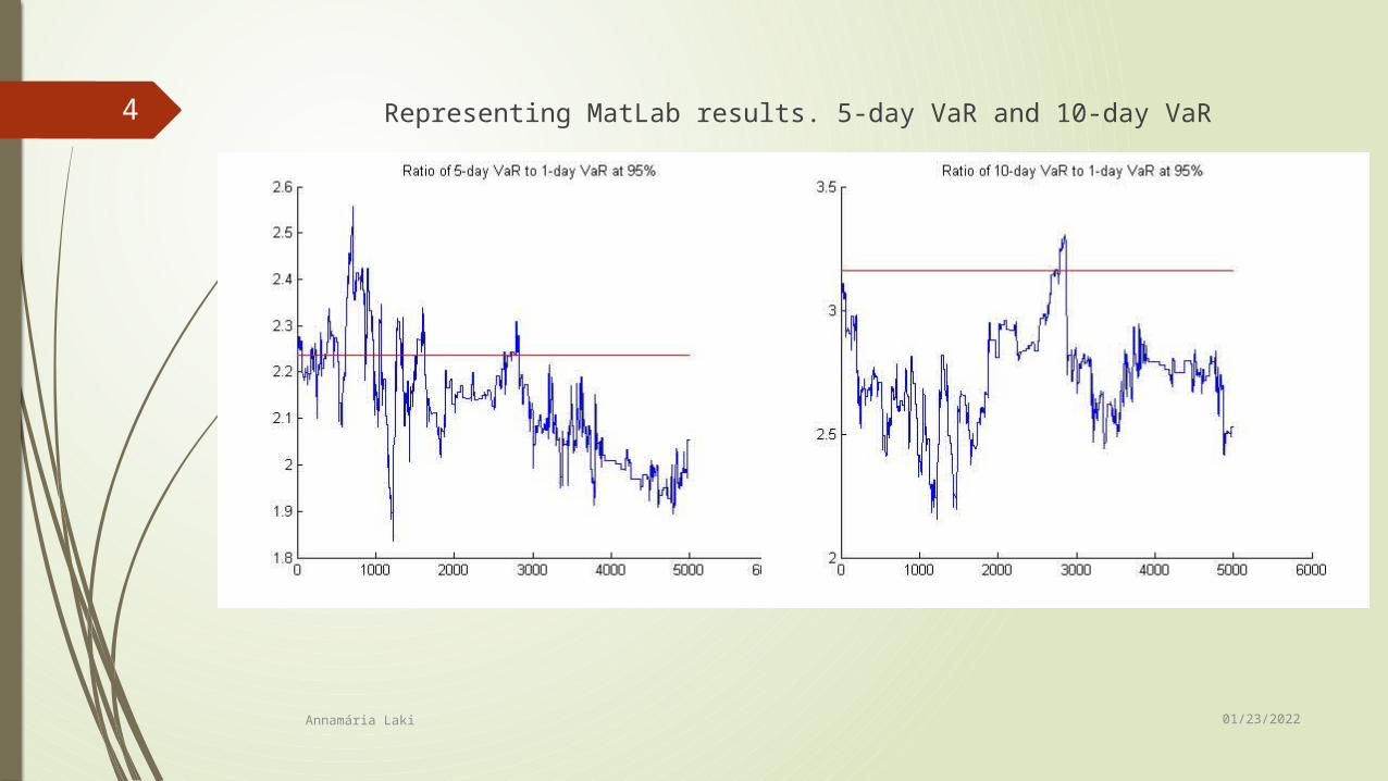
Sometimes regulators request market risk measures (eg. VaR) on a relatively long time horizon. The computations involving this length of time are meaningless, as there is no available good quality data. Imagine for example that a 2 week 99% VaR is requested. Even if we had 4 years of coherent data, we would have only 1 sample point for the 99% quantile. This is not sufficient. Therefore time-scaling techniques are used. This means that 1 day VaR is computed and it is multiplied by a scaling factor. Of course the sample will demonstrate a level of auto-correlation and will not have constant volatility, so this is theoretically incorrect. The question arises, how big of a mistake do we make if we use the square-root of time scaling. Can we convince ourselves and our audience (i.e. the regulators) that this approximation is acceptable? Can we present visually tangible / tractable diagrams to this effect? Can we at least say something about the tails of the distribution; say at 95% or 99%?

05/01/2023Annamária Laki
3 IntroductionOur last projects we wrote about Value at Risk and its computations using the historical method. In the first project we talked about 1-day VaR and the Regulatory Capital: 10-day VaR. But sometimes we do not have enough data, because there are 250 trading days means only 25 observation in a year. 4 years we have 100 observations, so we can not get a good 1% evaluation. So we must use 1-day VaR to compute 10-day VaR. We needed: • Portfolio ( eg. S&P500 )• Initial capital ( eg. $1000000 ) • Time-horizon: eg. 2013−2015 → number of days (2 years ≈ 500 days)• Confidence level: eg. 1% ↔ 99%. The confidence level shows us where is the minimum or maximum VaR takes place (eg. 1% of 2 years→ 5th place).• Important assumption on strategy: This is a constant portfolio.
05/01/2023Annamária Laki
4 Representing MatLab results. 5-day VaR and 10-day VaR

05/01/2023Annamária Laki
5In the second project we tried the "modified" Conditional Volatility VaR (CV-VaR) which gave us better estimation so it was an improvement over VaR, however I.I.D is still not achieved. The idea: assumed that PnL distribution depends on time through volatility.
Where F is distribution that „exists in the background”. So, we use time dependent volatility to get better estimated risk.To compute CV-VaR we need the same things as in the first project. • Portfolio (S&P500) (simplified compared to project 1) • Confidence-level • Time-horizon

05/01/2023Annamária Laki
6 Computation of CV-VaR:1. The portfolio’s Value (from Marks)2. PnL’s 3. Computing for example 30-day σt’s (StDEV) of the PnL.
4. After these steps we can compute the CV-VaR’s with different (mostly used 99% and 95%) confidence-levels.
where T: current day.Eg.:
: Percentile(PnL, 0.01)

05/01/2023Annamária Laki
7 PnL distribution is not heteroskedastic, so we should try modelling volatility.

05/01/2023Annamária Laki
8 VaR versus CV-VaR

05/01/2023Annamária Laki
9 Exponentially Weighted Moving Average (EWMA) In the third project we will see how EWMA works and how we can reach new results with it. 1. Calculate PnL’s. 2. Apply a weighting scheme. (0 < λ < 1) First, we calculate the PnL’s (or returns). That’s typically a series of daily returns where each return is expressed in continually compounded terms.

05/01/2023Annamária Laki
10 Today’s variance is a function of yesterday’s variance and yesterday’s return.
You’ll notice we needed to compute a long series of exponentially declining weights. We won’t do the math here, but one of the best features of the EWMA is that the entire series conveniently reduces to a recursive formula:
EWMA
Using the exponentially weighted moving average (EWMA), in which more recent returns have greater weight on the variance.

05/01/2023Annamária Laki
11 Firstly, we compare the results we got in Excel and after take a look in Matlab.
The EWMA method on the other hand gives more importance to recent information and hence places greater weight on more recent returns. For monthly data, the lambda parameter of the EWMA model is recommended to be set to 0.97.

05/01/2023Annamária Laki
12 I tried EWMA with different λ and I got these results.

05/01/2023Annamária Laki
13 EWMA with "the standard" λ = 0.9925 and λ = 0.8

05/01/2023Annamária Laki
14 Ewma with λ = 0.9925 and λ = 0.95

05/01/2023Annamária Laki
15 Note: with λ = 0.9925 and 30-day volatility with confidence level: 99%.
05/01/2023Annamária Laki
16 Summary
The main task: Regulators request credible market risk measures. This Project’s aim was to show one of the most used risk measure, the VaR and its "versions". I also tried modeling volatility (CV-VaR), and the last project showed results computing with EWMA.

05/01/2023Annamária Laki
17 Critics
Anyway, VaR is one of the most used risk measure, there are lots of different opinion has about using it. Is it works well? or can we measure risk with different conditions? (I mean if a portfolio does not normal distributed). Of course we can use, but maybe "the approach" will change so it can be an other solution. This solution is acceptable? or we should try another approach to reach our aim(s). Returns are very close to normal distribution but they are not. Critical market changes also affects VaR. Because of that facts sometimes risk underestimated or overestimated.

05/01/2023Annamária Laki
18 Future plans
Back testing such as:• One-tailed test • Kupiec’s two-tailed test

05/01/2023Annamária Laki
19 Acknowledgement
I would like to thank Áron Varga for the help and guidance he has given me. I know this topic is a little piece of risk management but I thank him for introducing me to the wonders and frustrations of this area.


