HAL Id: hal-01695424 https://hal.archives-ouvertes.fr/hal-01695424 Submitted on 29 Jan 2018 HAL is a multi-disciplinary open access archive for the deposit and dissemination of sci- entific research documents, whether they are pub- lished or not. The documents may come from teaching and research institutions in France or abroad, or from public or private research centers. L’archive ouverte pluridisciplinaire HAL, est destinée au dépôt et à la diffusion de documents scientifiques de niveau recherche, publiés ou non, émanant des établissements d’enseignement et de recherche français ou étrangers, des laboratoires publics ou privés. Application of the Recursive Finite Element Approach on 2D Periodic Structures under Harmonic Vibrations Reem Yassine, Faten Salman, Ali Al Shaer, Mohammad Hammoud, Denis Duhamel To cite this version: Reem Yassine, Faten Salman, Ali Al Shaer, Mohammad Hammoud, Denis Duhamel. Application of the Recursive Finite Element Approach on 2D Periodic Structures under Harmonic Vibrations. Evolutionary Computation, Massachusetts Institute of Technology Press (MIT Press), 2017, 5 (1), 10.3390/computation5010001. hal-01695424
Transcript
HAL Id: hal-01695424https://hal.archives-ouvertes.fr/hal-01695424
Submitted on 29 Jan 2018
HAL is a multi-disciplinary open accessarchive for the deposit and dissemination of sci-entific research documents, whether they are pub-lished or not. The documents may come fromteaching and research institutions in France orabroad, or from public or private research centers.
L’archive ouverte pluridisciplinaire HAL, estdestinée au dépôt et à la diffusion de documentsscientifiques de niveau recherche, publiés ou non,émanant des établissements d’enseignement et derecherche français ou étrangers, des laboratoirespublics ou privés.
Application of the Recursive Finite Element Approachon 2D Periodic Structures under Harmonic VibrationsReem Yassine, Faten Salman, Ali Al Shaer, Mohammad Hammoud, Denis
Duhamel
To cite this version:Reem Yassine, Faten Salman, Ali Al Shaer, Mohammad Hammoud, Denis Duhamel. Applicationof the Recursive Finite Element Approach on 2D Periodic Structures under Harmonic Vibrations.Evolutionary Computation, Massachusetts Institute of Technology Press (MIT Press), 2017, 5 (1),�10.3390/computation5010001�. �hal-01695424�
Application of the Recursive Finite Element Approachon 2D Periodic Structures under Harmonic VibrationsReem Yassine 1, Faten Salman 1, Ali Al Shaer 1, Mohammad Hammoud 1,* and Denis Duhamel 2
Academic Editor: Demos T. TsahalisReceived: 29 October 2016; Accepted: 16 December 2016; Published: 22 December 2016
Abstract: The frequency response function is a quantitative measure used in structural analysisand engineering design; hence, it is targeted for accuracy. For a large structure, a high number ofsubstructures, also called cells, must be considered, which will lead to a high amount of computationaltime. In this paper, the recursive method, a finite element method, is used for computing the frequencyresponse function, independent of the number of cells with much lesser time costs. The fundamentalprinciple is eliminating the internal degrees of freedom that are at the interface between a cell and itssucceeding one. The method is applied solely for free (no load) nodes. Based on the boundary andinterior degrees of freedom, the global dynamic stiffness matrix is computed by means of productsand inverses resulting with a dimension the same as that for one cell. The recursive method isdemonstrated on periodic structures (cranes and buildings) under harmonic vibrations. The methodyielded a satisfying time decrease with a maximum time ratio of 1
18 and a percentage difference of19%, in comparison with the conventional finite element method. Close values were attained at lowand very high frequencies; the analysis is supported for two types of materials (steel and plastic).The method maintained its efficiency with a high number of forces, excluding the case when all ofthe nodes are under loads.
Keywords: finite element analysis; recursive method; periodic structures; harmonic vibrations
1. Introduction
The study of structural dynamics is essential for understanding and evaluating the performance ofany engineering structure. Most structures vibrate. In operation, all machines, vehicles and buildingsare subjected to dynamic forces that cause vibrations. Very often, the vibrations have to be investigatedbecause they may cause an immediate problem. Whatever the reason, we need to quantify thestructural response in some way, so that its implication on factors such as performance and fatiguecan be evaluated. The frequency response function (FRF) will then be considered. These structuresmay have a uniform geometry or a periodic one. The frequency response function has acquired muchconsideration for high frequencies, since at small values, the system can be analyzed statically. Gettingthis function for the structures and system mentioned under a high range of angular frequencieswill lead to a large amount of computation time, since solving for the displacement vector requiresinversing the dynamic stiffness matrix at each angular frequency. As the number of substructures,also called cells, increases the computational cost increases. Hence, the approach emphasized in thisresearch presents a solution for this time issue.
Various methods were inspected to determine the frequency response for one-dimensionalstructures and their behavior as assembled for a two-dimensional element as a truss or frame. Original
numerical approaches were done by Dong and Aalami [1,2] to estimate the deformations on each pointon the cross-section by finite element analysis (conventional FEM).
One approach for structural analysis is the spectral finite element method (SFEM) that was mainlyused by Finnveden [3,4]. It considers general uniform structures with complex cross-sections andhandles all types of boundary conditions. The displacements in the cross-section are described bythe finite element method (FEM), while ordinary differential equations for 2D structures will expressthe variation along the axis of symmetry (x-axis) with a solution of the form ejkxU(y, z), where y andz are cross-sectional coordinates. A similar approach as SFEM called the dynamic stiffness method(DSM) is notably efficient for the study of excited structures under high frequencies [5]. It providesan economical solution with a much higher accuracy, since it divides the member into distinct elements.Both methods include similar steps till the extent of obtaining the dynamic stiffness matrix. DSMdefines a relationship between the nodal displacement and forces of the element using shape functions,in order to derive the dynamic stiffness matrix; whereas the SFEM uses the virtual work method toobtain the stiffness matrix, and the dynamic matrix will have a more laborious presentation, beinga function of the wave number. Structures made of plates and shells were examined by the SFEMapproach by Nilsson [6]. Birgersson [7–9] studied plane wave and fluid structure interaction. Gry andGavric [10,11] applied similar approaches for the detection of wave propagation on rails, wherethey calculated the relative dispersion relations. Similar techniques were interpreted by Bartoli andMarzani [12,13] for the purpose of computing the dispersion relations for damped structures ofarbitrary cross-sections and with symmetric elements.
Duhamel et al. [14] established a combined method between wave and finite element approachesfor investigating periodic structures; it has an advantage over the SFEM by its ease of operationsfor complex geometries and scattered materials. Lee et al. [15] utilized a compounded methodusing finite element and boundary element (FEBE) methods for studying periodic structuresmeshed non-periodically.
Reduced order models (ROMs) are mainly mathematically-inexpensive methods for solvingcomplex and large-scale dynamic problems by decreasing the model’s degrees of freedom. It gathersthe system’s responses under excitations, providing near real-life analysis, however with low accuracy.ROM was applied on mistuned bladed disks by Castanier et al. [16] for capturing localized modesand producing low order models with modest memory storage; it calculated relatively acceptableresults in comparison with FEM. The method was later improved by employing the Craig–Bamptoncomponent mode synthesis (CMS), which is an ROM-based technique yielding better mode accuracy;it required that at least one subspace iteration is executed (Bathe et al. [17]). CMS was then applied byZhou et al. [18] on dynamics analysis using non-uniform rational B-spline (NURBS) finite elementsto generate appropriate constructions of interfaced substructures. The method obtained a completestructural model consistent with the original model.
Duhamel [19,20] analyzed the frequency response by the recursive method (RM), on waveguidestructures, as beams, plates and tires. The beam was divided into two substructures. As the divisionnumber increases, a higher accuracy in the frequency response is obtained. He also studied someplates excited in the mid x and y positions. A simply supported plate is meshed, and then, its mass andstiffness matrices are extracted from ABAQUS and then inserted in MATLAB to obtain the frequencyresponse using the method studied. A similar method aiming to reduce the number of degrees offreedom under zero forces called the Guyan method is commonly used; however, it had been employedmainly for static analysis. Further, it neglects the inertia at the omitted DOF, hence being obsolete forstructures of high mass to stiffness ratios [21].
The paper provides a computational solving method for periodic structures that cannot bedesigned as waveguides, where the recursive method is studied for its efficiency. The recursive methodtends to ease the study of finite element analysis for complex structures. It is a computational methodthat computes the global dynamic stiffness matrix by products and inverses of matrices, resulting withthe same dimension as that of one cell. For a complex cross-section, the structure is sectioned and
Computation 2017, 5, 1 3 of 18
modeled in the conventional finite element software and then post-processed in MATLAB. RM tendsto eliminate any degrees of freedom (DOF) on the nodes that are not under study. Thus, a structure oftwo elements can be examined as one, on account of omitting the DOF at the boundaries between twoconsecutive cells, if there were no internal loads.
Two applications were examined under the illustrated method. The first application is wherethe RM is applied on 1D bar structures and demonstrating their manner as assembled in a craneunder harmonic and seismic loadings. The crane will be dealt with as a truss. A real-life example willbe considered, with a conservative number of elements. For the second application, the RM will beapplied on a building modeled as a frame. The seismic load will be designed as harmonic displacementat its base end. The truss and the frame are considered as 2D periodic structures.
Modal analysis is used to assess the dynamic properties of a structure by assessing the naturalfrequencies and their corresponding mode shapes. It was employed to determine the range offrequencies to be examined. FEM works on the full modes when computing the FRF, while RMwill only work on the modes that include the studied nodes. For example, in the presented study,the structure has no internal nodes for examination; hence, RM will consider the first mode only withthe two end nodes. Using the recursive method, a few computations are needed for finding a closeresponse compared to the number of computations used in the finite element analysis.
2. Recursive Method
2.1. Review
The recursive method is used to calculate the forced response of various types of structures,which might lead to a high consumption of computation. This method is used to compute the generaldynamic stiffness matrix with a much lower amount of computational time. Generally, the recursivemethod is a purely computational method, which computes the global dynamic stiffness matrix byproducts and inverses of matrices with the same dimensions as the dynamic stiffness matrix of a cell.
For a complex cross-section, the structure is sectioned and modeled in the conventional finiteelement software (ANSYS). Then, the mass, stiffness and damping matrices are extracted from ANSYS.
These matrices will be post-processed to give the dynamic stiffness matrix of the section understudy, after which, the global dynamic stiffness matrix of the whole structure will be figured fromthe recursive method. It will be obtained by means of products and inverses of the matrices with thedimension equal to that of the dynamic stiffness matrix of the section. This method tends to eliminateany degrees of freedom (DOF) on the nodes that are not under study. Thus, a structure of two elementscan be examined as one, on account of omitting the DOF at the boundaries between two consecutivecells, if there were no internal loads. In general, this method is applicable and effective when thestructure is not under a large number of forces.
The periodic structure that is divided into N cells is considered. The problem studied is undera point force excitation, having a response u. Following is a demonstration for the recursive method,numerically [14].
2.2. Behavior of One Cell
First, consider a one-cell element. The discrete dynamic stiffness matrix of a cell fora time-dependent e−iωt is given by: (
K− iωC−ω2M)
q = f , (1)
where i =√−1, ω is the angular frequency, K is the stiffness matrix, C is the damping matrix, M is the
mass matrix, q is the displacement vector and f is the loading vector.
Computation 2017, 5, 1 4 of 18
Thus, the dynamic stiffness matrix is:
D̃ = K− iωC−ω2M. (2)
Decomposing the degrees of freedom into the boundary (B) and interior (I), the resulting dynamicequation is: [
D̃BB D̃BID̃IB D̃I I
][qBqI
]=
[fB0
]. (3)
Then, eliminate the second row of Equation (3):
D̃IBqB + D̃I IqI = 0,qI = −D̃−1
I I D̃IBqB.(4)
The first row in Equation (3) will be:
fB = (D̃BB − D̃BI D̃−1I I D̃IB)qB. (5)
Thus, boundary conditions are only considered in the study. These conditions can be decomposedinto left (L) and right (R) for the relative nodes.
Equation (5) becomes:[fLfR
]=
[D(1)
LL D(1)LR
D(1)RL D(1)
RR
][qLqR
]= D(1)
[qLqR
], (6)
where D(1) is the dynamic stiffness matrix of a single cell.Since matrices K, C and M are symmetric, matrix D(1) will also be symmetric.
2.3. Behavior of Two Cells
For the assembly of two cells, consider the dynamic stiffness matrices A and B for Cell 1 andCell 2, respectively, as shown in Figure 1. The dynamic stiffness matrix is now denoted with D(2),which relates the DOF between the two sides (left and right). The dynamic stiffness matrix of thestructure is calculated using: f1
f2
f3
=
ALL ALR 0ARL ARR + BLL BLR
0 BRL BRR
q1
q2
q3
, (7)
since the interior side is taken with free loading f2 = 0. Thus, solving for the second row in the matrix:
q2 = −(ARR + BLL)−1(ARLq1 + BLRq3). (8)
The global dynamic stiffness matrix will then be:[f1
f3
]=
[ALL − (ARR + BLL)
−1 ARL −ALR(ARR + BLL)−1BLR
−BRL(ARR + BLL)−1 ARL BRR − BRL(ARR + BLL)
−1BRL
][
q1
q3
]=
[D(2)
LL D(2)LR
D(2)RL D(2)
RR
][q1
q3
]= D(2)
[q1
q3
],
(9)
where D(2) is the dynamic stiffness matrix of the two cells’ structure.
Computation 2017, 5, 1 5 of 18
Since matrices A and B are symmetric, matrix D(2) will also be symmetric. Therefore, we can write:
D(2) = {A, B}. (10)Computation 2017, 5, 1 5 of 18
Figure 1. Two-cell element.
2.4. General Case
Consider now a general case of a structure made of N cells, where it is under no load at its internal nodes. Denote its total dynamic stiffness matrix as ( ). Note that the structure is periodic and is isotropic. Firstly, consider a structure with identical cells; omit the internal degrees of freedom that are under no load. As stated in the foregoing method, the element of two cells is subsequently modeled as one cell. Hence, the current one-cell element will be assembled with a one-cell element that was previously a two-cell element. Proceeding with the N-cell structure, the outcome is a one-cell element that holds the nodes that are of interest for the assessment. For no restriction on the number of cells, the procedure is computed for steps. This accustomed number of steps will have a high effectiveness on saving the number of computations, when comparing with the conventional finite element analysis; since it is no longer required for the global assembly of the whole structure. The complete analysis is reviewed in Figure 2.
Figure 2. Element assembly in the recursive method.
In case the number of cells was not as a power of two, a binary representation will be used to model the system. For example, for N number of cells where N is not equal to a number with a power of two, it can be written in binary representation as = 11 = 1011 .
The system is solved as follows:
• Calculate the dynamic stiffness matrix for a structure of eight cells, decomposing them into four of two cells each.
• The studied structure is then assembled with a structure of two cells, studied previously. • The resulting matrix is assembled with a structure of one cell.
This approach can be resumed by: ( ) = { ( ), ( ) , ( )}. (11)
This method provides an easy approach for the computations of a structure with a large number of cells under harmonic vibrations. After applying the force and displacement boundary conditions, the response for the node subjected to forced vibrations is studied and detected for the frequency response function.
Figure 1. Two-cell element.
2.4. General Case
Consider now a general case of a structure made of N cells, where it is under no load at itsinternal nodes. Denote its total dynamic stiffness matrix as D(N). Note that the structure is periodicand is isotropic. Firstly, consider a structure with identical cells; omit the internal degrees of freedomthat are under no load. As stated in the foregoing method, the element of two cells is subsequentlymodeled as one cell. Hence, the current one-cell element will be assembled with a one-cell elementthat was previously a two-cell element. Proceeding with the N-cell structure, the outcome is a one-cellelement that holds the nodes that are of interest for the assessment. For no restriction on the numberof cells, the procedure is computed for log2N steps. This accustomed number of steps will havea high effectiveness on saving the number of computations, when comparing with the conventionalfinite element analysis; since it is no longer required for the global assembly of the whole structure.The complete analysis is reviewed in Figure 2.
Computation 2017, 5, 1 5 of 18
Figure 1. Two-cell element.
2.4. General Case
Consider now a general case of a structure made of N cells, where it is under no load at its internal nodes. Denote its total dynamic stiffness matrix as ( ). Note that the structure is periodic and is isotropic. Firstly, consider a structure with identical cells; omit the internal degrees of freedom that are under no load. As stated in the foregoing method, the element of two cells is subsequently modeled as one cell. Hence, the current one-cell element will be assembled with a one-cell element that was previously a two-cell element. Proceeding with the N-cell structure, the outcome is a one-cell element that holds the nodes that are of interest for the assessment. For no restriction on the number of cells, the procedure is computed for steps. This accustomed number of steps will have a high effectiveness on saving the number of computations, when comparing with the conventional finite element analysis; since it is no longer required for the global assembly of the whole structure. The complete analysis is reviewed in Figure 2.
Figure 2. Element assembly in the recursive method.
In case the number of cells was not as a power of two, a binary representation will be used to model the system. For example, for N number of cells where N is not equal to a number with a power of two, it can be written in binary representation as = 11 = 1011 .
The system is solved as follows:
• Calculate the dynamic stiffness matrix for a structure of eight cells, decomposing them into four of two cells each.
• The studied structure is then assembled with a structure of two cells, studied previously. • The resulting matrix is assembled with a structure of one cell.
This approach can be resumed by: ( ) = { ( ), ( ) , ( )}. (11)
This method provides an easy approach for the computations of a structure with a large number of cells under harmonic vibrations. After applying the force and displacement boundary conditions, the response for the node subjected to forced vibrations is studied and detected for the frequency response function.
Figure 2. Element assembly in the recursive method.
In case the number of cells was not as a power of two, a binary representation will be used tomodel the system. For example, for N number of cells where N is not equal to a number with a powerof two, it can be written in binary representation as N = 11 = 1011b.
The system is solved as follows:
• Calculate the dynamic stiffness matrix for a structure of eight cells, decomposing them into fourof two cells each.
• The studied structure is then assembled with a structure of two cells, studied previously.• The resulting matrix is assembled with a structure of one cell.
This approach can be resumed by:
D(11) ={{
D(8), D(2)}
, D(1)}
. (11)
This method provides an easy approach for the computations of a structure with a large numberof cells under harmonic vibrations. After applying the force and displacement boundary conditions,the response for the node subjected to forced vibrations is studied and detected for the frequencyresponse function.
Computation 2017, 5, 1 6 of 18
3. Applications
Periodic structures were examined in this paper. For the first application, 1D bar structures areassembled in a crane. Excitation and seismic loading will be examined on cranes, where it will bedealt with as a truss. On the other hand, the application of the recursive method will be on 2D frame,where a harmonic displacement is loaded at its base nodes (model of seismic load). The frame isconsidered as a 2D periodic structure.
After computing the FRF conventionally (using harmonic analysis in ANSYS), the response will becompared to that determined from the recursive method. Note that a FULL analysis method was usedin ANSYS, where it uses the full system’s matrices for computing the response; this will lead to a morecomprehensive and detailed approach. RM is defined by a self-written MATLAB code where it takesthe K, M and C matrices of a one cell from ANSYS for the frame structure. However, these matriceswill be calculated manually for the truss application. Then, the matrices will be assembled reaching Ncells, recursively. The dynamic stiffness matrix will be obtained by products and inverses of matriceswith the same dimension as the dynamic stiffness matrix of one cell. Nodes that are under no load ornot under study will be omitted using this method. Hence, internal degrees of freedom between theadjacent cells will be removed using the RM.
3.1. Truss Application
A truss is an element structure consisting of two or more bar elements, connected to each otherby pins, by which each pin will support rotations around its axis only. Cranes are modeled as a truss,where this will be studied under forced vibrations and seismic loading. A freestanding crane isconsidered as a periodic structure where the repeated cell is shown in Figure 3. The global nodes arenumbered as in the displayed order in ANSYS.
Computation 2017, 5, 1 6 of 18
3. Applications
Periodic structures were examined in this paper. For the first application, 1D bar structures are assembled in a crane. Excitation and seismic loading will be examined on cranes, where it will be dealt with as a truss. On the other hand, the application of the recursive method will be on 2D frame, where a harmonic displacement is loaded at its base nodes (model of seismic load). The frame is considered as a 2D periodic structure.
After computing the FRF conventionally (using harmonic analysis in ANSYS), the response will be compared to that determined from the recursive method. Note that a FULL analysis method was used in ANSYS, where it uses the full system’s matrices for computing the response; this will lead to a more comprehensive and detailed approach. RM is defined by a self-written MATLAB code where it takes the K, M and C matrices of a one cell from ANSYS for the frame structure. However, these matrices will be calculated manually for the truss application. Then, the matrices will be assembled reaching N cells, recursively. The dynamic stiffness matrix will be obtained by products and inverses of matrices with the same dimension as the dynamic stiffness matrix of one cell. Nodes that are under no load or not under study will be omitted using this method. Hence, internal degrees of freedom between the adjacent cells will be removed using the RM.
3.1. Truss Application
A truss is an element structure consisting of two or more bar elements, connected to each other by pins, by which each pin will support rotations around its axis only. Cranes are modeled as a truss, where this will be studied under forced vibrations and seismic loading. A freestanding crane is considered as a periodic structure where the repeated cell is shown in Figure 3. The global nodes are numbered as in the displayed order in ANSYS.
Figure 3. Repeated cell in the truss.
The bar elements will differ by their cross-sectional areas, since the vertical bars hold larger loads; then, its cross-sectional area is larger than those of the horizontal and inclined bars. Hence, each element is oriented differently relative to the global coordinate system.
The element equation is expressed as: + ̅ − ∆ = , (12)
where = √−1, is the angular velocity, is the local stiffness matrix, ̅ is the local damping matrix, is the local mass matrix, ∆ is the local displacement vector and is the local loading vector.
The truss element will have two degrees of freedom (DOF) at each node: translations in the nodal x and y directions.
The bar element under study is a steel bar with characteristics represented in Table 1.
Figure 3. Repeated cell in the truss.
The bar elements will differ by their cross-sectional areas, since the vertical bars hold largerloads; then, its cross-sectional area is larger than those of the horizontal and inclined bars. Hence,each element is oriented differently relative to the global coordinate system.
The element equation is expressed as:
[Ke+ iωCe −ω2Me
] [∆e]= [Fe
], (12)
where i =√−1, ω is the angular velocity, Ke is the local stiffness matrix, Ce is the local damping matrix,
Me is the local mass matrix, ∆e is the local displacement vector and Fe is the local loading vector.The truss element will have two degrees of freedom (DOF) at each node: translations in the nodal
x and y directions.The bar element under study is a steel bar with characteristics represented in Table 1.
Computation 2017, 5, 1 7 of 18
Table 1. Bar element characteristics.
Young’s Modulus of Elasticity E = 200 GPaDensity ρ = 7800 kg
m3
Damping Ratio ζ = 0.004 [22]Larger Cross-Sectional Area A1 = 0.001175 m2
Smaller Cross-Sectional Area A2 = 2.91× 10⁻⁴ m2
Length for the Vertical and Horizontal Bars, Respectively l = 1.5− 2 m
Referenced to real-life applications, freestanding tower cranes with fixed foundations and noundercarriage supports are modeled as cranes with the repeated cell mentioned before, and they areonly repeated 16 times with a total length of 53.65 m, including the foundation height. All dimensionsare assumed relative to actual values.
Both types of loadings will be applied to the same crane structure presented, with the samerepeated cell and type of material employed. Hence, the structures relative to the two differentloadings will have equal stiffness, mass and damping matrices. The dynamic stiffness matrix isobtained due to the discussed approach, without the need for global assembly.
3.1.1. Truss under Forced Vibration at the Last Node
Ce is taken for two different types of damping:
• Rayleigh damping:Ce
= αKe+ βMe, (13)
where α and β are calculated from the natural frequencies and the relative damping ratio.The natural frequencies taken are the first two natural frequencies, with their relative modeshapes shown in Figure 4; determined by modal analysis. The damping ratio for steel materialused in a footbridge damping is ζ = 0.004 [22].
• Hysteretic damping:
The dynamic stiffness matrix is demonstrated as:
De = (1 + 0.01 ∗ i)Ke −ω2Me. (14)
Computation 2017, 5, 1 7 of 18
Table 1. Bar element characteristics.
Young’s Modulus of Elasticity = 200GPa Density = 7800 kgm
Damping Ratio = 0.004 [22] Larger Cross-Sectional Area 1 = 0.001175m Smaller Cross-Sectional Area 2 = 2.91 ∗ 10 m Length for the Vertical and Horizontal Bars, Respectively = 1.5 − 2m
Referenced to real-life applications, freestanding tower cranes with fixed foundations and no
undercarriage supports are modeled as cranes with the repeated cell mentioned before, and they are only repeated 16 times with a total length of 53.65m , including the foundation height. All dimensions are assumed relative to actual values.
Both types of loadings will be applied to the same crane structure presented, with the same repeated cell and type of material employed. Hence, the structures relative to the two different loadings will have equal stiffness, mass and damping matrices. The dynamic stiffness matrix is obtained due to the discussed approach, without the need for global assembly.
3.1.1. Truss under Forced Vibration at the Last Node ̅ is taken for two different types of damping:
• Rayleigh damping: ̅ = + , (13)
where and are calculated from the natural frequencies and the relative damping ratio. The natural frequencies taken are the first two natural frequencies, with their relative mode shapes shown in Figure 4; determined by modal analysis. The damping ratio for steel material used in a footbridge damping isζ = 0.004 [22].
(a) (b)
Figure 4. Mode shapes for the natural frequencies. (a) The first mode shape with a modal frequency of = 1.0235Hz; (b) the second mode shape with a modal frequency of = 5.7271Hz.
Figure 4. Mode shapes for the natural frequencies. (a) The first mode shape with a modal frequency off n1 = 1.0235 Hz; (b) the second mode shape with a modal frequency of f n2 = 5.7271 Hz .
Computation 2017, 5, 1 8 of 18
The crane interpreted is illustrated in Figure 5. The last nodes of interest are under harmonicvibrations for F = F0e−iωt, where F0 = 1 N. The fixed foundation will remove the degrees of freedomon the first two nodes in the global system, and the matrix is assembled upon a relationship betweena cell and its consecutive one. The periodic structure is computed under a range of driving frequencies,for the purpose of estimating the frequency response function at the excited node.
Computation 2017, 5, 1 8 of 18
• Hysteretic damping:
The dynamic stiffness matrix is demonstrated as: = (1 + 0.01 ∗ ) − . (14)
The crane interpreted is illustrated in Figure 5. The last nodes of interest are under harmonic vibrations for = , where = 1N . The fixed foundation will remove the degrees of freedom on the first two nodes in the global system, and the matrix is assembled upon a relationship between a cell and its consecutive one. The periodic structure is computed under a range of driving frequencies, for the purpose of estimating the frequency response function at the excited node.
Figure 5. Crane under forced excitation.
3.1.2. Truss under Seismic Load
The truss application is applied under a second type of loading for the investigation of the frequency response function under a range of frequencies. The crane structure will be studied under hysteretic damping solely, represented by the previously shown dynamic stiffness matrix (14). The first two nodes are subjected to seismic load, which is modeled as a harmonic displacement of= , where = 0.01m on the base of the structure, as shown in Figure 6.
Figure 6. Crane under seismic load.
3.2. Frame Application under Seismic Load
Frames are structures that have a combination of beams resisting loads. Such structures are modeled to overcome large moments developed due to the applied loading. The connected node acquires three DOF, preventing displacement in the y-direction and rotations in the x- and z-direction. A building under seismic load is modeled as a frame. Timoshenko beams will be
Figure 5. Crane under forced excitation.
3.1.2. Truss under Seismic Load
The truss application is applied under a second type of loading for the investigation of thefrequency response function under a range of frequencies. The crane structure will be studied underhysteretic damping solely, represented by the previously shown dynamic stiffness matrix (14). The firsttwo nodes are subjected to seismic load, which is modeled as a harmonic displacement of d = d0e−iωt,where d0 = 0.01 m on the base of the structure, as shown in Figure 6.
Computation 2017, 5, 1 8 of 18
• Hysteretic damping:
The dynamic stiffness matrix is demonstrated as: = (1 + 0.01 ∗ ) − . (14)
The crane interpreted is illustrated in Figure 5. The last nodes of interest are under harmonic vibrations for = , where = 1N . The fixed foundation will remove the degrees of freedom on the first two nodes in the global system, and the matrix is assembled upon a relationship between a cell and its consecutive one. The periodic structure is computed under a range of driving frequencies, for the purpose of estimating the frequency response function at the excited node.
Figure 5. Crane under forced excitation.
3.1.2. Truss under Seismic Load
The truss application is applied under a second type of loading for the investigation of the frequency response function under a range of frequencies. The crane structure will be studied under hysteretic damping solely, represented by the previously shown dynamic stiffness matrix (14). The first two nodes are subjected to seismic load, which is modeled as a harmonic displacement of= , where = 0.01m on the base of the structure, as shown in Figure 6.
Figure 6. Crane under seismic load.
3.2. Frame Application under Seismic Load
Frames are structures that have a combination of beams resisting loads. Such structures are modeled to overcome large moments developed due to the applied loading. The connected node acquires three DOF, preventing displacement in the y-direction and rotations in the x- and z-direction. A building under seismic load is modeled as a frame. Timoshenko beams will be
Figure 6. Crane under seismic load.
3.2. Frame Application under Seismic Load
Frames are structures that have a combination of beams resisting loads. Such structures aremodeled to overcome large moments developed due to the applied loading. The connected nodeacquires three DOF, preventing displacement in the y-direction and rotations in the x- and z-direction.A building under seismic load is modeled as a frame. Timoshenko beams will be studied, having
Computation 2017, 5, 1 9 of 18
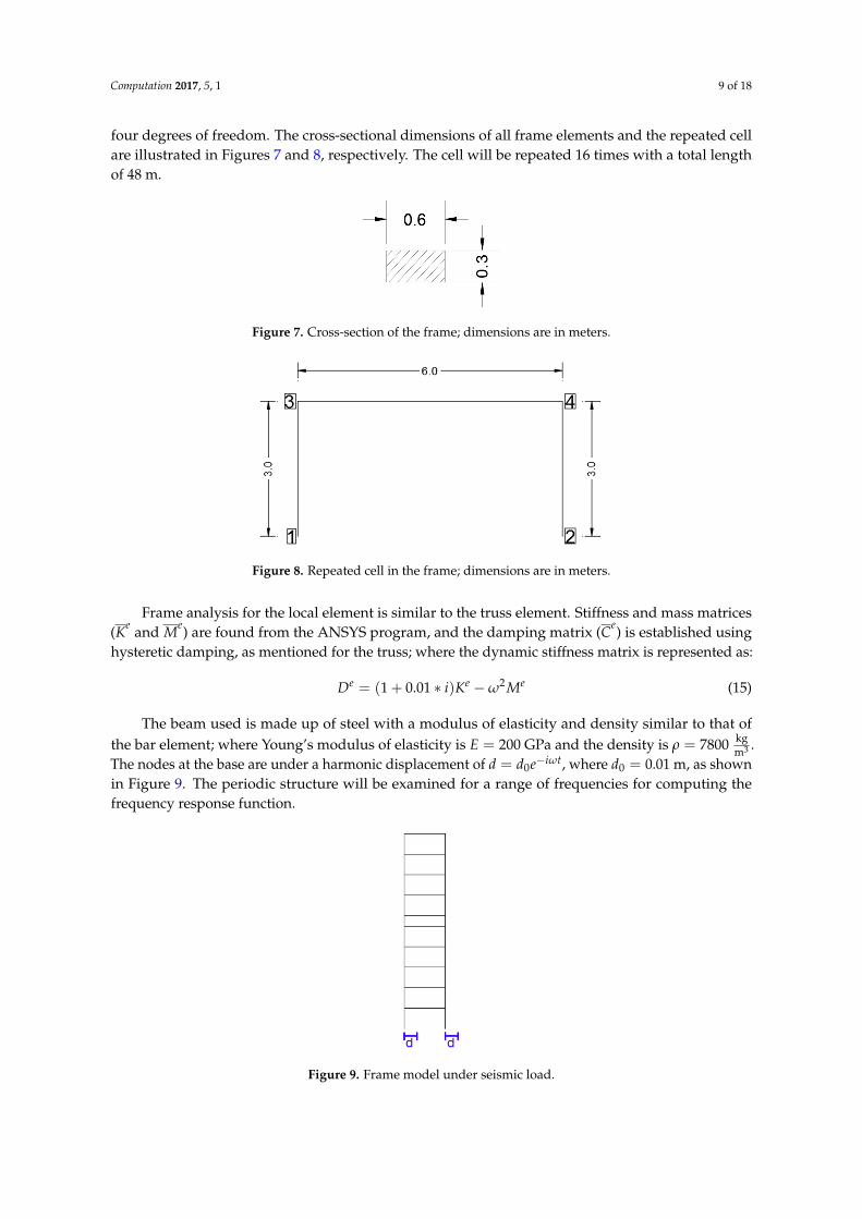
four degrees of freedom. The cross-sectional dimensions of all frame elements and the repeated cellare illustrated in Figures 7 and 8, respectively. The cell will be repeated 16 times with a total lengthof 48 m.
Computation 2017, 5, 1 9 of 18
studied, having four degrees of freedom. The cross-sectional dimensions of all frame elements and the repeated cell are illustrated in Figures 7 and 8, respectively. The cell will be repeated 16 times with a total length of48m.
Figure 7. Cross-section of the frame; dimensions are in meters.
Figure 8. Repeated cell in the frame; dimensions are in meters.
Frame analysis for the local element is similar to the truss element. Stiffness and mass matrices ( and ) are found from the ANSYS program, and the damping matrix ( ̅ ) is established using hysteretic damping, as mentioned for the truss; where the dynamic stiffness matrix is represented as: = (1 + 0.01 ∗ ) − . (15)
The beam used is made up of steel with a modulus of elasticity and density similar to that of the bar element; where Young’s modulus of elasticity is = 200GPa and the density is = 7800 . The nodes at the base are under a harmonic displacement of = , where = 0.01m, as shown in Figure 9. The periodic structure will be examined for a range of frequencies for computing the frequency response function.
Figure 9. Frame model under seismic load.
Figure 7. Cross-section of the frame; dimensions are in meters.
Computation 2017, 5, 1 9 of 18
studied, having four degrees of freedom. The cross-sectional dimensions of all frame elements and the repeated cell are illustrated in Figures 7 and 8, respectively. The cell will be repeated 16 times with a total length of48m.
Figure 7. Cross-section of the frame; dimensions are in meters.
Figure 8. Repeated cell in the frame; dimensions are in meters.
Frame analysis for the local element is similar to the truss element. Stiffness and mass matrices ( and ) are found from the ANSYS program, and the damping matrix ( ̅ ) is established using hysteretic damping, as mentioned for the truss; where the dynamic stiffness matrix is represented as: = (1 + 0.01 ∗ ) − . (15)
The beam used is made up of steel with a modulus of elasticity and density similar to that of the bar element; where Young’s modulus of elasticity is = 200GPa and the density is = 7800 . The nodes at the base are under a harmonic displacement of = , where = 0.01m, as shown in Figure 9. The periodic structure will be examined for a range of frequencies for computing the frequency response function.
Figure 9. Frame model under seismic load.
Figure 8. Repeated cell in the frame; dimensions are in meters.
Frame analysis for the local element is similar to the truss element. Stiffness and mass matrices(Ke and Me) are found from the ANSYS program, and the damping matrix (Ce) is established usinghysteretic damping, as mentioned for the truss; where the dynamic stiffness matrix is represented as:
De = (1 + 0.01 ∗ i)Ke −ω2Me (15)
The beam used is made up of steel with a modulus of elasticity and density similar to that ofthe bar element; where Young’s modulus of elasticity is E = 200 GPa and the density is ρ = 7800 kg
m3 .The nodes at the base are under a harmonic displacement of d = d0e−iωt, where d0 = 0.01 m, as shownin Figure 9. The periodic structure will be examined for a range of frequencies for computing thefrequency response function.
Computation 2017, 5, 1 9 of 18
studied, having four degrees of freedom. The cross-sectional dimensions of all frame elements and the repeated cell are illustrated in Figures 7 and 8, respectively. The cell will be repeated 16 times with a total length of48m.
Figure 7. Cross-section of the frame; dimensions are in meters.
Figure 8. Repeated cell in the frame; dimensions are in meters.
Frame analysis for the local element is similar to the truss element. Stiffness and mass matrices ( and ) are found from the ANSYS program, and the damping matrix ( ̅ ) is established using hysteretic damping, as mentioned for the truss; where the dynamic stiffness matrix is represented as: = (1 + 0.01 ∗ ) − . (15)
The beam used is made up of steel with a modulus of elasticity and density similar to that of the bar element; where Young’s modulus of elasticity is = 200GPa and the density is = 7800 . The nodes at the base are under a harmonic displacement of = , where = 0.01m, as shown in Figure 9. The periodic structure will be examined for a range of frequencies for computing the frequency response function.
Figure 9. Frame model under seismic load.
Figure 9. Frame model under seismic load.
Computation 2017, 5, 1 10 of 18
4. Results
The FRF obtained from the recursive method will be compared to that using a conventional finiteelement program (ANSYS). The elapsed time for each application is measured and collated betweenthe FEM and RM. The PC machine utilized for finite element analysis runs on an Intel Core i7-4500Uwith a clk (clock) speed of 2.40 GHz and 8.00 GB of RAM.
4.1. Truss Application under Forced Vibration
The results for the crane structure made up of 16 repeated cells under Rayleigh damping isdemonstrated in Figure 10, and a zoomed-in presentation was done to illustrate the difference inachieving close results between low and high frequencies. The results represent the variation of themodulus of displacement logarithmically with respect to the range of frequencies for the last node,excited under harmonic forced vibration.
Computation 2017, 5, 1 10 of 18
4. Results
The FRF obtained from the recursive method will be compared to that using a conventional finite element program (ANSYS). The elapsed time for each application is measured and collated between the FEM and RM. The PC machine utilized for finite element analysis runs on an Intel Core i7-4500U with a clk (clock) speed of 2.40 GHz and 8.00 GB of RAM.
4.1. Truss Application under Forced Vibration
The results for the crane structure made up of 16 repeated cells under Rayleigh damping is demonstrated in Figure 10, and a zoomed-in presentation was done to illustrate the difference in achieving close results between low and high frequencies. The results represent the variation of the modulus of displacement logarithmically with respect to the range of frequencies for the last node, excited under harmonic forced vibration.
Figure 10. Displacement of the excited node under Rayleigh damping for the truss application that is
applied to forced vibration. The graph is logarithmically scaled. : low frequencies; : high frequencies. RM, recursive method.
Figure 11 illustrates the normalized percentage error between the RM and FEM methods in the low and high frequencies domains, evaluating approximate low frequencies as values less than 50 Hz. In the low frequency domain, the structure most likely behaves as in the static equilibrium, where the effect of the driving frequencies is still minimal on the response (low effect as if = 0). The evaluated percentages were very small for < 50Hz. However, for > 50Hz, the structure is most likely showing dynamic behavior. High frequencies will estimate a larger percentage range since then, the effect of becomes recognizable and influential, increasing the mass effect − . Very high frequencies estimated better results since beyond that for cases where the structure’s properties (mass and stiffness) are high (complete structure estimated recursively), the inverse of the dynamic stiffness matrix will result in closer FRF. The response under hysteretic damping is shown in Figure 12.
Figure 10. Displacement of the excited node under Rayleigh damping for the truss application that
is applied to forced vibration. The graph is logarithmically scaled.
Computation 2017, 5, 1 10 of 18
4. Results
The FRF obtained from the recursive method will be compared to that using a conventional finite element program (ANSYS). The elapsed time for each application is measured and collated between the FEM and RM. The PC machine utilized for finite element analysis runs on an Intel Core i7-4500U with a clk (clock) speed of 2.40 GHz and 8.00 GB of RAM.
4.1. Truss Application under Forced Vibration
The results for the crane structure made up of 16 repeated cells under Rayleigh damping is demonstrated in Figure 10, and a zoomed-in presentation was done to illustrate the difference in achieving close results between low and high frequencies. The results represent the variation of the modulus of displacement logarithmically with respect to the range of frequencies for the last node, excited under harmonic forced vibration.
Figure 10. Displacement of the excited node under Rayleigh damping for the truss application that is
applied to forced vibration. The graph is logarithmically scaled. : low frequencies; : high frequencies. RM, recursive method.
Figure 11 illustrates the normalized percentage error between the RM and FEM methods in the low and high frequencies domains, evaluating approximate low frequencies as values less than 50 Hz. In the low frequency domain, the structure most likely behaves as in the static equilibrium, where the effect of the driving frequencies is still minimal on the response (low effect as if = 0). The evaluated percentages were very small for < 50Hz. However, for > 50Hz, the structure is most likely showing dynamic behavior. High frequencies will estimate a larger percentage range since then, the effect of becomes recognizable and influential, increasing the mass effect − . Very high frequencies estimated better results since beyond that for cases where the structure’s properties (mass and stiffness) are high (complete structure estimated recursively), the inverse of the dynamic stiffness matrix will result in closer FRF. The response under hysteretic damping is shown in Figure 12.
: low frequencies;
Computation 2017, 5, 1 10 of 18
4. Results
The FRF obtained from the recursive method will be compared to that using a conventional finite element program (ANSYS). The elapsed time for each application is measured and collated between the FEM and RM. The PC machine utilized for finite element analysis runs on an Intel Core i7-4500U with a clk (clock) speed of 2.40 GHz and 8.00 GB of RAM.
4.1. Truss Application under Forced Vibration
The results for the crane structure made up of 16 repeated cells under Rayleigh damping is demonstrated in Figure 10, and a zoomed-in presentation was done to illustrate the difference in achieving close results between low and high frequencies. The results represent the variation of the modulus of displacement logarithmically with respect to the range of frequencies for the last node, excited under harmonic forced vibration.
Figure 10. Displacement of the excited node under Rayleigh damping for the truss application that is
applied to forced vibration. The graph is logarithmically scaled. : low frequencies; : high frequencies. RM, recursive method.
Figure 11 illustrates the normalized percentage error between the RM and FEM methods in the low and high frequencies domains, evaluating approximate low frequencies as values less than 50 Hz. In the low frequency domain, the structure most likely behaves as in the static equilibrium, where the effect of the driving frequencies is still minimal on the response (low effect as if = 0). The evaluated percentages were very small for < 50Hz. However, for > 50Hz, the structure is most likely showing dynamic behavior. High frequencies will estimate a larger percentage range since then, the effect of becomes recognizable and influential, increasing the mass effect − . Very high frequencies estimated better results since beyond that for cases where the structure’s properties (mass and stiffness) are high (complete structure estimated recursively), the inverse of the dynamic stiffness matrix will result in closer FRF. The response under hysteretic damping is shown in Figure 12.
: highfrequencies. RM, recursive method.
Figure 11 illustrates the normalized percentage error between the RM and FEM methods in thelow and high frequencies domains, evaluating approximate low frequencies as values less than 50 Hz.In the low frequency domain, the structure most likely behaves as in the static equilibrium, where theeffect of the driving frequencies is still minimal on the response (low effect as if ω = 0). The evaluatedpercentages were very small for f < 50 Hz. However, for f > 50 Hz, the structure is most likelyshowing dynamic behavior. High frequencies will estimate a larger percentage range since then, theeffect of ω2 becomes recognizable and influential, increasing the mass effect Ke − ω2Me. Very highfrequencies estimated better results since beyond that for cases where the structure’s properties (massand stiffness) are high (complete structure estimated recursively), the inverse of the dynamic stiffnessmatrix will result in closer FRF. The response under hysteretic damping is shown in Figure 12.
Computation 2017, 5, 1 11 of 18Computation 2017, 5, 1 11 of 18
Figure 11. Normalized percentage of error between FEM and RM for a range of frequencies.
Figure 12. Displacement of the excited node under hysteretic damping for the truss application that is applied to forced vibration. The graph is logarithmically scaled.
The difference in the elapsed time for each method is presented in Table 2. The time elapsed for getting the frequency response in both damping cases is much higher using the finite element method than that of the recursive method. The finite element analysis took approximately 18-times more than the recursive method. Larger time differences between the two damping types are anticipated to be calculated for more complex structures where the number of DOF is very large.
More high frequency peaks are shown for hysteretic damping, due to its complete material dependency. The peaks are caused by imperfections in material elasticity, in which the reaction of the material to changes is dependent on its past reactions to change.
Table 2. Time comparison between the two methods, for the truss application under forced vibrations.
Method Elapsed Time (s)
Time Ratio Rayleigh Damping Hysteretic Damping
RM 0.618 0.638 = 118 FEM 11.26 11.43
Figure 11. Normalized percentage of error between FEM and RM for a range of frequencies.
Computation 2017, 5, 1 11 of 18
Figure 11. Normalized percentage of error between FEM and RM for a range of frequencies.
Figure 12. Displacement of the excited node under hysteretic damping for the truss application that is applied to forced vibration. The graph is logarithmically scaled.
The difference in the elapsed time for each method is presented in Table 2. The time elapsed for getting the frequency response in both damping cases is much higher using the finite element method than that of the recursive method. The finite element analysis took approximately 18-times more than the recursive method. Larger time differences between the two damping types are anticipated to be calculated for more complex structures where the number of DOF is very large.
More high frequency peaks are shown for hysteretic damping, due to its complete material dependency. The peaks are caused by imperfections in material elasticity, in which the reaction of the material to changes is dependent on its past reactions to change.
Table 2. Time comparison between the two methods, for the truss application under forced vibrations.
Method Elapsed Time (s)
Time Ratio Rayleigh Damping Hysteretic Damping
RM 0.618 0.638 = 118 FEM 11.26 11.43
Figure 12. Displacement of the excited node under hysteretic damping for the truss application that isapplied to forced vibration. The graph is logarithmically scaled.
The difference in the elapsed time for each method is presented in Table 2. The time elapsed forgetting the frequency response in both damping cases is much higher using the finite element methodthan that of the recursive method. The finite element analysis took approximately 18-times more thanthe recursive method. Larger time differences between the two damping types are anticipated to becalculated for more complex structures where the number of DOF is very large.
Table 2. Time comparison between the two methods, for the truss application under forced vibrations.
MethodElapsed Time (s)
Time RatioRayleigh Damping Hysteretic Damping
RM 0.618 0.638 tRMtFEM
=̃ 118FEM 11.26 11.43
Computation 2017, 5, 1 12 of 18
More high frequency peaks are shown for hysteretic damping, due to its complete materialdependency. The peaks are caused by imperfections in material elasticity, in which the reaction of thematerial to changes is dependent on its past reactions to change.
4.2. Truss Application under Seismic Load
The frequency response function found from the recursive method using hysteretic damping willbe compared to that using the conventional finite element program (ANSYS), and the results are shownin Figure 13. The values calculated demonstrate the variation of the displacement under a range offrequencies for the first node that is applied to harmonic displacement. Hysteretic damping is knownto be completely material dependent. This is due to some imperfection of the elasticity of the material,in which the reaction of the material to changes is dependent on its past reactions to change.
Computation 2017, 5, 1 12 of 18
4.2. Truss Application under Seismic Load
The frequency response function found from the recursive method using hysteretic damping will be compared to that using the conventional finite element program (ANSYS), and the results are shown in Figure 13. The values calculated demonstrate the variation of the displacement under a range of frequencies for the first node that is applied to harmonic displacement. Hysteretic damping is known to be completely material dependent. This is due to some imperfection of the elasticity of the material, in which the reaction of the material to changes is dependent on its past reactions to change.
Figure 13. Displacement of the last top node of the truss structure under seismic load, applied to hysteretic damping. The graph is logarithmically scaled.
The time ratio calculated between the two methods is approximately 1:22, as in Table 3. The calculated elapsed time shows that the finite element method took approximately 22-times more than the recursive method to compute the FRF for the crane structure under hysteretic damping.
Table 3. Time comparison between the two methods, for the truss application under seismic load.
Method Elapsed Time (s) Time RatioRM 0.505 = 122
FEM 11.08
4.3. Frame Application under Seismic Load
The results found using the recursive method and the conventional finite element software (ANSYS) for determining the frequency response function are presented in Figure 14. It displays the logarithmic varying displacement of the first bottom node that is excited under harmonic displacement. The modulus of displacement is studied for a range of frequencies.
The time ratio calculated between two methods is approximately 1/31.6, as shown in Table 4. The measured time elapsed for the two comparing methods reveals that the FEM took approximately 32-times more than the RM to compute the FRF for the frame structure under seismic load.
Figure 13. Displacement of the last top node of the truss structure under seismic load, applied tohysteretic damping. The graph is logarithmically scaled.
The time ratio calculated between the two methods is approximately 1:22, as in Table 3.The calculated elapsed time shows that the finite element method took approximately 22-times morethan the recursive method to compute the FRF for the crane structure under hysteretic damping.
Table 3. Time comparison between the two methods, for the truss application under seismic load.
Method Elapsed Time (s) Time Ratio
RM 0.505 tRMtFEM
=̃ 122FEM 11.08
4.3. Frame Application under Seismic Load
The results found using the recursive method and the conventional finite element software(ANSYS) for determining the frequency response function are presented in Figure 14. It displays thelogarithmic varying displacement of the first bottom node that is excited under harmonic displacement.The modulus of displacement is studied for a range of frequencies.
The time ratio calculated between two methods is approximately 1/31.6, as shown in Table 4.The measured time elapsed for the two comparing methods reveals that the FEM took approximately32-times more than the RM to compute the FRF for the frame structure under seismic load.
Computation 2017, 5, 1 13 of 18Computation 2017, 5, 1 13 of 18
Figure 14. Displacement of the last top node for the frame application under seismic loading, applied to hysteretic damping. The graph is logarithmically scaled.
Table 4. Time comparison between the two methods for the frame application.
Method Elapsed Time (s) Time RatioRM 2.078 = 131.6 FEM 65.80
4.4. Analysis
4.4.1. Periodic Structures Having Steel Material
The results for the two different applications under harmonic vibrations showed that RM calculated values are close, but slightly higher than the values of the FEM. For low and high frequencies, the modulus of displacement of the RM showed nearer values than at frequencies that cannot be considered as high. Note that the finite element analysis was taken as the reference method. The percentage difference between the two approaches for the two applications is established in Table 5.
Rayleigh damping is defined as the type of damping that is frequency dependent, and it depends on the natural frequencies for defining its equation. However, hysteretic damping is a material-dependent type of damping; thus, it has the advantage of minimizing the effect of the driving frequency on the response. These two types of damping were studied on the truss application under forced excitations, solely. The graph relative to the Rayleigh damping demonstrates that the response was damped at lower frequency than that of the other type of damping.
Table 5. Percentage difference.
Type of Application Type of Loading Type of Damping
Building Harmonic displacement Hysteretic damping 1:1:2000 18.920%
Figure 14. Displacement of the last top node for the frame application under seismic loading, appliedto hysteretic damping. The graph is logarithmically scaled.
Table 4. Time comparison between the two methods for the frame application.
Method Elapsed Time (s) Time Ratio
RM 2.078 tRMtFEM
=̃ 131.6FEM 65.80
4.4. Analysis
4.4.1. Periodic Structures Having Steel Material
The results for the two different applications under harmonic vibrations showed that RMcalculated values are close, but slightly higher than the values of the FEM. For low and highfrequencies, the modulus of displacement of the RM showed nearer values than at frequencies thatcannot be considered as high. Note that the finite element analysis was taken as the reference method.The percentage difference between the two approaches for the two applications is established in Table 5.
Rayleigh damping is defined as the type of damping that is frequency dependent, and itdepends on the natural frequencies for defining its equation. However, hysteretic damping isa material-dependent type of damping; thus, it has the advantage of minimizing the effect of thedriving frequency on the response. These two types of damping were studied on the truss applicationunder forced excitations, solely. The graph relative to the Rayleigh damping demonstrates that theresponse was damped at lower frequency than that of the other type of damping.
Table 5. Percentage difference.
Type ofApplication Type of Loading Type of Damping Range of
Building Harmonic displacement Hysteretic damping 1:1:2000 18.920%
The maximum natural frequency is defined as the greatest value of the frequency that canillustrate a physical understanding of the structure’s response via the mode shape demonstratedby modal analysis. Further, this value of the natural frequency will determine the maximum rangeof frequencies to be examined. Concerning the truss structure, for natural frequencies greater than
Computation 2017, 5, 1 14 of 18
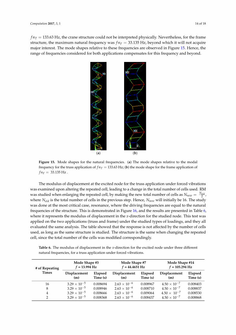
f nT = 133.63 Hz, the crane structure could not be interpreted physically. Nevertheless, for the framestructure, the maximum natural frequency was f nF = 33.135 Hz, beyond which it will not acquiremajor interest. The mode shapes relative to these frequencies are observed in Figure 15. Hence, therange of frequencies considered for both applications compensates for this frequency and beyond.
Computation 2017, 5, 1 14 of 18
The maximum natural frequency is defined as the greatest value of the frequency that can illustrate a physical understanding of the structure’s response via the mode shape demonstrated by modal analysis. Further, this value of the natural frequency will determine the maximum range of frequencies to be examined. Concerning the truss structure, for natural frequencies greater than = 133.63Hz, the crane structure could not be interpreted physically. Nevertheless, for the frame structure, the maximum natural frequency was = 33.135Hz, beyond which it will not acquire major interest. The mode shapes relative to these frequencies are observed in Figure 15. Hence, the range of frequencies considered for both applications compensates for this frequency and beyond.
(a) (b)
Figure 15. Mode shapes for the natural frequencies. (a) The mode shapes relative to the modal frequency for the truss application of = 133.63Hz; (b) the mode shape for the frame application of = 33.135Hz. The modulus of displacement at the excited node for the truss application under forced
vibrations was examined upon altering the repeated cell, leading to a change in the total number of cells used. RM was studied when enlarging the repeated cell, by making the new total number of cells as = , where is the total number of cells in the previous step. Hence, will initially be 16. The study was done at the most critical case, resonance, where the driving frequencies are equal to the natural frequencies of the structure. This is demonstrated in Figure 16, and the results are presented in Table 6, where it represents the modulus of displacement in the x-direction for the studied node. This test was applied on the two applications (truss and frame) under the studied types of loadings, and they all evaluated the same analysis. The table showed that the response is not affected by the number of cells used, as long as the same structure is studied. The structure is the same when changing the repeated cell, since the total number of the cells was modified correspondingly.
Figure 15. Mode shapes for the natural frequencies. (a) The mode shapes relative to the modalfrequency for the truss application of f nT = 133.63 Hz; (b) the mode shape for the frame application off nF = 33.135 Hz .
The modulus of displacement at the excited node for the truss application under forced vibrationswas examined upon altering the repeated cell, leading to a change in the total number of cells used. RMwas studied when enlarging the repeated cell, by making the new total number of cells as Nnew = Nold
2 ,where Nold is the total number of cells in the previous step. Hence, Nnew will initially be 16. The studywas done at the most critical case, resonance, where the driving frequencies are equal to the naturalfrequencies of the structure. This is demonstrated in Figure 16, and the results are presented in Table 6,where it represents the modulus of displacement in the x-direction for the studied node. This test wasapplied on the two applications (truss and frame) under the studied types of loadings, and they allevaluated the same analysis. The table showed that the response is not affected by the number of cellsused, as long as the same structure is studied. The structure is the same when changing the repeatedcell, since the total number of the cells was modified correspondingly.
Table 6. The modulus of displacement in the x-direction for the excited node under three differentnatural frequencies, for a truss application under forced vibrations.
Computation 2017, 5, 1 15 of 18Computation 2017, 5, 1 15 of 18
(a) (b) (c)
Figure 16. The repeated cells are presented where: (a) the new repeated cell is double the previous one and it is repeated eight times; (b) the new repeated cell consists of four-times the old cell, and it is repeated four times; (c) the cell will be repeated two times.
Table 6. The modulus of displacement in the x-direction for the excited node under three different natural frequencies, for a truss application under forced vibrations.
4.4.2. Periodic Structures Having Plastic Material
This was also investigated for a plastic material (PVC: polyvinyl chloride) having Young’s modulus of elasticity of = 3.4GPaand a density of = 1330 for the two applications under forced excitation and seismic loading. The results are shown in Table 7. The values measured had the same inspection, determining the acceptance of the analysis deduced, by which for low and high driving frequencies, the response was more acceptable than intermediate frequencies in comparison with FEM. The percentage difference between the two approaches for the two applications when PVC material is assigned are established in Table 8. The table shows that the measured elapsed time for the FEM took approximately 22× more time than the RM to compute the FRF for the truss structure under the two types of loadings. Moreover, FEM consumed a high amount of time in the computations during the implementations of the frame structure under seismic load, where it took 150× more time than the RM to compute the FRF.
Table 7. The modulus of displacement in the x-direction for the excited node under three different natural frequencies, for a truss application under forced vibrations, upon assignment of PVC.
Figure 16. The repeated cells are presented where: (a) the new repeated cell is double the previousone and it is repeated eight times; (b) the new repeated cell consists of four-times the old cell, and it isrepeated four times; (c) the cell will be repeated two times.
4.4.2. Periodic Structures Having Plastic Material
This was also investigated for a plastic material (PVC: polyvinyl chloride) having Young’smodulus of elasticity of E = 3.4 GPa and a density of ρ = 1330 kg
m3 for the two applications underforced excitation and seismic loading. The results are shown in Table 7. The values measured hadthe same inspection, determining the acceptance of the analysis deduced, by which for low and highdriving frequencies, the response was more acceptable than intermediate frequencies in comparisonwith FEM. The percentage difference between the two approaches for the two applications when PVCmaterial is assigned are established in Table 8. The table shows that the measured elapsed time forthe FEM took approximately 22×more time than the RM to compute the FRF for the truss structureunder the two types of loadings. Moreover, FEM consumed a high amount of time in the computationsduring the implementations of the frame structure under seismic load, where it took 150×more timethan the RM to compute the FRF.
Table 7. The modulus of displacement in the x-direction for the excited node under three differentnatural frequencies, for a truss application under forced vibrations, upon assignment of PVC.
Table 8. Percentage difference for the PVC material.
Type ofApplication
Type ofLoading
Type ofDamping
Time Elapsed (s) Time Ratio( tRM
tFEM)
Range of FrequencyStudied (Hz)
PercentageDifferenceFEM RM
CraneForced
vibrationsHystereticdamping 12.64 0.572 =̃ 1
22 1:700 3.3584%
Harmonicdisplacement
Hystereticdamping 11.03 0.509 =̃ 1
22 1:700 17.4930%
Building Harmonicdisplacement
Hystereticdamping 86.34 0.575 =̃ 1
151 1:800 14.3027%
4.4.3. The Effect of the Number of Forces Applied
The first study on the crane included behavioral examination of the excited node under forcedvibrations. Loads were applied on one node exclusively. This section includes studying theeffectiveness of this approach for periodic structures under a large number of forces. The effectof the number of forces is investigated in three different cases, in an increasing order of multiplyingby two. A force is added at the mid-span of the truss structure in addition to the load exerted at itstop. Then, the number of loads increases to four, after applying two excitations at 1
4 L and 34 L. Further
increasing includes the addition of four more forces, resulting in a periodic structure applied to eightloads that are equal in magnitude and uniformly distanced. Table 9 presents the resultant outcomesfor the relevant test.
Table 9. Results upon adding different numbers of forces distributed equally over the periodic structure.
# of ForcesAdded
Elapsed Time (s)Time Ratio tRM
tFEM
Range of FrequencyStudied (Hz)
Range of PercentageDifferenceFEM RM
2 70.70 0.6680 =̃ 1106 1:1:700 9 ≤ %E ≤ 12
4 84.46 0.4909 =̃ 1172 1:1:700 8 ≤ %E ≤ 10
8 73.85 0.6727 =̃ 1110 1:1:700 9 ≤ %E ≤ 11
The elapsed times consumed by the FEM and the RM are displayed and compared; the time ratioshows the high efficacy of applying this method on a high number of forces. The percentage differencewas measured at each excited node, and the results show a low difference between the two methods.However, there were two excited nodes that showed a high difference upon interpretations. The twonodes are the last excited node when four forces were applied, and the other is the mid-excited nodeupon eight force excitations, where the percentage difference exceeded 50%. Farther studies should beemployed to illustrate a relation between the numbers of forces that can be applied with the lengthof the periodic structure, while maintaining significant effectiveness. Supplementary expectationsare that when the forces are engaged with every node, the method will not be feasible for calculatingthe frequency response function, since the advantage of removing the internal nodes recursively willbe obsolete.
5. Conclusions
In this paper, a further study was done on structures that cannot be designed as waveguides.Cranes and buildings were modeled as trusses and frames, respectively, under various loading.Trusses and frames have in their structural composition the inability to guide waves along theirlongitudinal axis. Waveguides are used in various types of applications and have different methodsfor accurate computations. However, structures that are not considered as waveguides consumevarious applications, as well, but there are no different numerical methods for easier, faster andprecise computations.
Computation 2017, 5, 1 17 of 18
The recursive method is an approach used for calculating the frequency response function ofgeneral periodic structures. In spite of the element’s complexity, a recursive method can be employedon all types of periodic structures, as long as the internal nodes are under no load. For findinga satisfying result, a high number of cells must be considered, which will lead to a large number ofcomputations. This method provides a solution close to that obtained from the reference method(FEM), and it decreases the time consumption. The time consumed for a steel material was observedto a have a range of ratios between 1:18 and 1:31, depending on the type of cells and the load exerted.Displacement values were nearer to that of the finite element method at low and very high frequencies.The percentage difference for the structures studied under various types of loading does not exceed19%. Nevertheless, different materials were studied to have further support of the analysis. The plasticmaterial had much lower time ratios, in the range between 1:22 and 1:151, while the relative percentagedifference did not exceed 17%. This difference is due to the inverse of the dynamic stiffness matrix,which will lead to a slight numerical difference between the finite element method and the recursivemethod. Upon varying the number of forces, the time ratio lied in the range of 1:106 till 1:172, with a lowpercentage difference.
Future examinations include studying the effectiveness of this approach for periodic structuresunder a large number of forces. Expectations are that when the forces are engaged with every node,the method will not be feasible for calculating the frequency response function, since the advantage ofremoving the internal nodes recursively will be obsolete. Further studies include the types of cells to berepeated and the effect on the frequency response function. Moreover, a more applicable solution maybe calculated by changing the type of element from linear to quadratic; therefore, vibrations at internalnodes can be computed. Otherwise, an element with a greater mesh size should be examined, since theincrease in the mesh size will display the response for the internal nodes. The effect of the frequencyon the modulus of displacement will be also inspected, and more complex periodic structures will beinterpreted. Unsteady states in heat transfer problems may be evaluated for complex fin geometries.
Author Contributions: Reem Yassine and Faten Salman wrote most of this paper. Ali Al Shaer and MohammadHammoud contributed to the numerical simulations. Denis Duhamel contributed to the finalizing of the paperand the reviewing process.
Conflicts of Interest: The authors declare no conflict of interest.
References
1. Dong, S.B.; Nelson, R.B. On natural vibrations and waves in laminated orthotropic plates. J. Appl. Mech.1972, 39, 739–745. [CrossRef]
2. Aalami, B. Waves in prismatic guides of arbitrary cross section. J. Appl. Mech. 1973, 40, 1067–1072. [CrossRef]3. Finnveden, S. Finite Element Techniques for the Evaluation of Energy Flow Parameters: Keynote Lecture.
In Proceedings of the Novem2000 Conference, Lyon, France, 2–4 November 2000.4. Finnveden, S. Evaluation of modal density and group velocity by a finite element method. J. Sound Vib. 2004,
273, 51–75. [CrossRef]5. Yu, C.P.; Roesset, J.M. Dynamic stiffness matrices for linear members with distributed mass. J. Appl. Sci. Eng.
2001, 4, 253–264.6. Nilsson, C.M. Waveguide Finite Elements for Thin-Waled Structures. Licentiate Thesis, KTH Royal Institute
of Technology, Stockholm, Sweden, 2002.7. Birgersson, F. Prediction of Random Vibration Using Spectral Methods. Ph.D. Thesis, KTH Royal Institute of
Technology, TRITA-AVE, Stockholm, Sweden, 2003; p. 30.8. Birgersson, F.; Finnveden, S.; Nilsson, C.M. A spectral super element for modelling of plate vibration. Part 1:
General theory. J. Sound Vib. 2005, 287, 297–314. [CrossRef]9. Birgersson, F.; Finnveden, S. A spectral super element for modelling of plate vibration. Part 2: Turbulence
excitation. J. Sound Vib. 2005, 287, 315–328. [CrossRef]10. Gry, L. Dynamic modelling of railway track based on wave propagation. J. Sound Vib. 1996, 195, 477–505.
11. Gavric, L. Computation of propagative waves in free rail using finite element technique. J. Sound Vib. 1995,185, 531–543. [CrossRef]
12. Bartoli, I.; Marzani, A.; Lanza di Scalea, F.; Viola, E. Modelling wave propagation in damed waveguide ofarbitrary cross-section. J. Sound Vib. 2006, 295, 685–707. [CrossRef]
13. Marzani, A.; Viola, E.; Bartoli, I.; Lanza di Scalea, F.; Rizzo, P. A semi-analytical finite element formulation formodelling stress wave propagation in axisymmertic damped waveguides. J. Sound Vib. 2008, 318, 488–505.[CrossRef]
14. Duhamel, D.; Mace, B.R.; Brennan, M.J. Finite element analysis of the vibrations of waveguides and periodicstructures. J. Sound Vib. 2004, 294, 205–220. [CrossRef]
15. Lee, S.C.; Rawatt, V.; Lee, J.F. A hybrid finite/boundary element method for periodic structures onnon-periodic meshes using an interior penalty formulation for Maxwell’s equations. J. Comput. Phys.2010, 229, 4934–4951. [CrossRef]
16. Castanier, M.P.; Ottarsson, G.; Pierre, C. A Reduced Order Modeling Technique for Mistuned Bladed Disks.J. Vib. Acoust. 1997, 119, 439–447. [CrossRef]
17. Bathe, K.J.; Dong, J. Component mode synthesis with subspace iterations for controlled accuracy of frequencyand mode shape solutions. Comput. Struct. 2014, 139, 28–32. [CrossRef]
18. Zhou, K.; Liang, G.; Tang, J. Component mode synthesis order-reduction for dynamic analysis of structuremodeled with NURBS finite element. J. Vib. Acoust. 2016, 138, 021016. [CrossRef]
19. Duhamel, D. A recursive approach for the finite element computation of waveguides. J. Sound Vib. 2009, 323,163–172. [CrossRef]
20. Duhamel, D.; Erlicher, S.; Nguyen, H.H. A recursive finite element method for comuting tyre vibrations.Eur. J. Comput. Mech. 2011, 20, 9–27.
21. Guyan, R.J. Reduction of stiffness and mass matrices. AIAA J. 1965, 3, 380–387. [CrossRef]22. Bachmann, H.; Ammann, W.J.; Deischl, F.; Eisenmann, J.; Floegl, J.; Hirsch, G.H.; Klein, G.K.; Lande, G.J.;
Mahrenholtz, O.; Natke, H.G.; et al. Vibration Problems in Structures: Practical Guidelines; Institut für Baustatikund Konstruktion (IBK): Basel, Switzerland, 1995.