Application of the Strictly Contractive Peaceman-Rachford Splitting Method to Multi-block Separable Convex Programming Bingsheng He, Han Liu, Juwei Lu, and Xiaoming Yuan Abstract Recently, a strictly contractive Peaceman-Rachford splitting method (SC- PRSM) was proposed to solve a convex minimization model with linear constraints and a separable objective function which is the sum of two functionals without cou- pled variables. We show by an example that the SC-PRSM cannot be directly ex- tended to the case where the objective function is the sum of three or more function- als. To solve such a multi-block model, if we treat its variables and functions as two groups and directly apply the SC-PRSM, then at least one of SC-PRSM subprob- lems involves more than one function and variable which might not be easy to solve. One way to improve the solvability for this direct application of the SC-PRSM is to further decompose such a subproblem so as to generate easier decomposed sub- problems which could potentially be simple enough to have closed-form solutions for some specific applications. The curse accompanying this improvement in solv- ability is that the SC-PRSM with further decomposed subproblems is not necessarily convergent, either. We will show its divergence by the same example. Our main goal in this chapter is to show that the convergence can be guaranteed if the further de- Bingsheng He International Centre of Management Science and Engineering, School of Management and En- gineering, and Department of Mathematics, Nanjing University, Nanjing, 200093, China, e-mail: [email protected]. This author was supported by the NSFC grant 91130007 and the MOEC fund 20110091110004., Han Liu Department of Operations Research and Financial Engineering, Princeton University, Princeton, NJ 08544, USA, e-mail: [email protected]. This author was supported by NSF Grant III–1116730. Juwei Lu Department of Operations Research and Financial Engineering, Princeton University, Princeton, NJ 08544, USA, e-mail: [email protected]Xiaoming Yuan Department of Mathematics, Hong Kong Baptist University, Hong Kong, e-mail: xmyuan@ hkbu.edu.hk. This author was supported by the General Research Fund from Research Grants Council of Hong Kong: 12302514. 1
Transcript
Application of the Strictly ContractivePeaceman-Rachford Splitting Method toMulti-block Separable Convex Programming
Bingsheng He, Han Liu, Juwei Lu, and Xiaoming Yuan
Abstract Recently, a strictly contractive Peaceman-Rachford splitting method (SC-PRSM) was proposed to solve a convex minimization model with linear constraintsand a separable objective function which is the sum of two functionals without cou-pled variables. We show by an example that the SC-PRSM cannot be directly ex-tended to the case where the objective function is the sum of three or more function-als. To solve such a multi-block model, if we treat its variables and functions as twogroups and directly apply the SC-PRSM, then at least one of SC-PRSM subprob-lems involves more than one function and variable which might not be easy to solve.One way to improve the solvability for this direct application of the SC-PRSM isto further decompose such a subproblem so as to generate easier decomposed sub-problems which could potentially be simple enough to have closed-form solutionsfor some specific applications. The curse accompanying this improvement in solv-ability is that the SC-PRSM with further decomposed subproblems is not necessarilyconvergent, either. We will show its divergence by the same example. Our main goalin this chapter is to show that the convergence can be guaranteed if the further de-
Bingsheng HeInternational Centre of Management Science and Engineering, School of Management and En-gineering, and Department of Mathematics, Nanjing University, Nanjing, 200093, China, e-mail:[email protected]. This author was supported by the NSFC grant 91130007 and the MOECfund 20110091110004.,
Han LiuDepartment of Operations Research and Financial Engineering, Princeton University, Princeton,NJ 08544, USA, e-mail: [email protected]. This author was supported by NSF GrantIII–1116730.
Juwei LuDepartment of Operations Research and Financial Engineering, Princeton University, Princeton,NJ 08544, USA, e-mail: [email protected]
Xiaoming YuanDepartment of Mathematics, Hong Kong Baptist University, Hong Kong, e-mail: [email protected]. This author was supported by the General Research Fund from Research GrantsCouncil of Hong Kong: 12302514.
1
2 Bingsheng He, Han Liu, Juwei Lu, and Xiaoming Yuan
composed subproblems of the direct application of the SC-PRSM are regularized bythe proximal regularization. As a result, an SC-PRSM-based splitting algorithm withprovable convergence and easy implementability is proposed for multi-block con-vex minimization models. We analyze the convergence for the derived algorithm, in-cluding proving its global convergence and establishing its worst-case convergencerate measured by the iteration complexity. The efficiency of the new algorithm isillustrated by testing some applications arising in image processing and statisticallearning.
We first consider a convex minimization model with linear constraints and an objec-tive function in form of the sum of two functions without coupled variables:
minθ1(x)+θ2(y) | Ax+By = b, x ∈X ,y ∈ Y , (1)
where A ∈ ℜm×n1 , B ∈ ℜm×n2 , X ⊂ ℜn1 and Y ⊂ ℜn2 are closed convex sets,θ1 and θ2 are convex but not necessarily smooth functions. A typical applicationof (1) is that θ1 refers to a data-fidelity term and θ2 denotes a regularization term.Concrete applications of the model (1) arise frequently in many areas such as imageprocessing, statistical learning, computer vision, etc., where θ1 and θ2 could befurther specified by particular physical or industrial elaboration for a given scenario.
A benchmark solver for (1) is the alternating direction method of multipliers(ADMM) originally proposed in [23] (see also [6, 19]). Applying to the solution ofproblem (1), ADMM reads as
xk+1 = argmin
θ1(x)− (λ k)T (Ax+Byk−b)+ β
2 ‖Ax+Byk−b‖2∣∣ x ∈X
,
yk+1 = argmin
θ2(y)− (λ k)T (Axk+1 +By−b)+ β
2 ‖Axk+1 +By−b‖2∣∣ y ∈ Y
,
λ k+1 = λ k−β (Axk+1 +Byk+1−b),(2)
where λ k,λ k+1 ∈ ℜm are Lagrange multipliers and β > 0 is a penalty parameter.Throughout we assume that the penalty parameter β is fixed. As analyzed inten-sively in [18, 22] (and observed for the first time in [6]), the scheme (2) can be re-garded as an application of the Douglas-Rachford splitting method (DRSM), whichis well known in the PDE literature (see [12, 34]). The ADMM algorithm can alsobe regarded as a splitting version of the augmented Lagrangian method (ALM), in-troduced in [31, 41]; and it outperforms the direct application of the ALM in thatthe functions θ1 and θ2 are treated individually and thus the splitted subproblems in(2) could be much easier than the original ALM subproblems. Recently, this featurehas found impressive applications in a variety of areas, and it has inspired a “renais-
SC-PRSM to Multi-block Separable Convex Programming 3
sance” of ADMM in the literature. We refer to [4, 13, 20] for some review papers ofthe ADMM.
In addition to DRSM, some authors (see e.g. [24, 33]) have also investigated howto apply the Peacemen-Rachford splitting method (PRSM) (another well-knownoperator-splitting method, introduced in [39] and further discussed in, e.g., [34])to the separable convex minimization model (1). This motivation was further en-hanced by the observation that “very often PRSM is faster than DRSM wheneverit converges”, as pointed out in [2, 21, 22]. More specifically, PRSM applied to thesolution of (1) leads to
xk+1 = argmin
θ1(x)− (λ k)T (Ax+Byk−b)+ β
2 ‖Ax+Byk−b‖2∣∣ x ∈X
,
λ k+ 12 = λ k−β (Axk+1 +Byk−b),
yk+1 = argmin
θ2(y)− (λ k+ 12 )T (Axk+1 +By−b)+ β
2 ‖Axk+1 +By−b‖2∣∣ y ∈ Y
,
λ k+1 = λ k+ 12 −β (Axk+1 +Byk+1−b),
(3)which differs from the DRSM scheme (2) in that it updates the Lagrange multiplierstwice at each iteration. The PRSM algorithm has the disadvantage of being “lessstable than DRSM”, although it does outperform it in most situations where it isconvergent (see [34, 21]). In [26], this disadvantage was explained by the fact thatthe sequence generated by PRSM is not necessarily strictly contractive with respectto the solution set of (1) (assuming that this set is non-empty), while the sequencegenerated by DRSM is strictly contractive. Note that we follow the definition of astrictly contractive sequence given in [3]. In [10], a counterexample showing thatthe sequence generated by PRSM could maintain a constant distance to the solutionset was constructed. Thus, the PRSM algorithm (3) is not necessarily convergent.To reinforce the robustness of the PRSM algorithm (3), with provable convergenceproperty, the following strictly contractive variant of (3) (denoted by SC-PRSM)was proposed in [26]:
xk+1 = argmin
θ1(x)− (λ k)T (Ax+Byk−b)+ β
2 ‖Ax+Byk−b‖2∣∣ x ∈X
,
λ k+ 12 = λ k−αβ (Axk+1 +Byk−b),
yk+1 = argmin
θ2(y)− (λ k+ 12 )T (Axk+1 +By−b)+ β
2 ‖Axk+1 +By−b‖2∣∣ y ∈ Y
,
λ k+1 = λ k+ 12 −αβ (Axk+1 +Byk+1−b),
(4)where α ∈ (0,1). It was shown in [26] that the parameter α plays the role of en-forcing the sequence generated by (4) to be strictly contractive with respect to thesolution set of (1). Hence, the convergence of the SC-PRSM algorithm (4) can beproved by standard techniques in the literature (e.g [3]). In [26], the efficiency of theSC-PRSM algorithm (4) was also verified numerically.
In addition to the model (1), we encounter numerous applications where the ob-jective function has a higher degree of separability such that it can be expressed asthe sum of more than two functionals without coupled variables. To expose our mainidea with easier notation, let us only focus on the case with three functionals in theobjective
4 Bingsheng He, Han Liu, Juwei Lu, and Xiaoming Yuan
minθ1(x)+θ2(y)+θ3(z) | Ax+By+Cz = b, x ∈X ,y ∈ Y ,z ∈Z , (5)
where A ∈ℜm×n1 , B ∈ℜm×n2 , C ∈ℜm×n3 , b ∈ℜm, X ⊂ℜn1 and Y ⊂ℜn2 , Z ⊂ℜn3 are closed convex sets, θi (i = 1,2,3) are convex functions. Throughout, the so-lution set of (5) is assumed to be nonempty. Some typical applications in form of (5)include the robust principal component analysis model with noisy and incompletedata in [44], the latent variable Gaussian graphical model selection in [7], the robustalignment model for linearly correlated images in [40], the quadratic discriminantanalysis model in [36] and many others.
To solve (5), one natural idea is to directly extend the ADMM algorithm (2). Theresulting scheme is
xk+1 = argminLβ (x,yk,zk,λ k)
∣∣ x ∈X,
yk+1 = argminLβ (xk+1,y,zk,λ k)
∣∣ y ∈ Y,
zk+1 = argminLβ (xk+1,yk+1,z,λ k)
∣∣ z ∈Z,
λ k+1 = λ k−β (Axk+1 +Byk+1 +Czk+1−b),
(6)
where Lβ (x,y,z,λ ) is the augmented Lagrangian function of (5) defined as
and where λ k,λ k+1 ∈ℜm are Lagrange multipliers, β > 0 is a penalty parameter. Al-gorithm (6) is a direct extension of the ADMM algorithm (2); from now on we willdenote (6) by E-ADMM; E-ADMM perfectly inherits the advantage of the ADMMalgorithm (2), and it can be obtained by simply decomposing the ALM subprobleminto 3 subproblems in Gauss-Seidel manner at each iteration. Empirically, it oftenworks very well, see e.g. [40, 44] for some applications. However, it was shownin [9] that the E-ADMM (6) is not necessarily convergent. We refer to [27, 28] forsome methods whose main common idea is to ensure the convergence via correctingthe output of (6) appropriately.
Similarly, for solving the multi-block convex minimization model (5), we maywish to consider directly extending the SC-PRSM scheme (4) as
xk+1 = argmin
θ1(x)− (λ k)T (Ax+Byk +Czk−b)+ β
2 ‖Ax+Byk +Czk−b‖2∣∣ x ∈X
,
λk+ 1
3 = λ k−αβ (Axk+1 +Byk +Czk−b),yk+1 = argmin
θ2(y)− (λ k+ 1
3 )T (Axk+1 +By+Czk−b)+ β
2 ‖Axk+1 +By+Czk−b‖2∣∣ y ∈ Y
,
λk+ 2
3 = λk+ 1
3 −αβ (Axk+1 +Byk+1 +Czk−b),zk+1 = argmin
θ3(z)− (λ k+ 2
3 )T (Axk+1 +Byk+1 +Cz−b)+ β
2 ‖Axk+1 +Byk+1 +Cz−b‖2∣∣ z ∈Z
,
λ k+1 = λk+ 2
3 −αβ (Axk+1 +Byk+1 +Czk+1−b).(7)
Hereafter, we denote algorithm (7) by E-SC-PRSM. Our first purpose is to show thatE-SC-PRSM is not necessarily convergent, as shown in Section 5.2, the method toprove this property being similar to the one used in [9]. From this possible diver-gence property, E-SC-PRSM (7) cannot be used directly to solve (5).
SC-PRSM to Multi-block Separable Convex Programming 5
Alternatively, one may wish to use the original SC-PRSM algorithm (4) directlyby regarding θ2(y)+θ3(z) as the second functional in (1) and regrouping (y,z) and(B,C) as the second variable and coefficient matrix in (1), respectively. The directapplication of the SC-PRSM algorithm (4) to the solution of problem (5) leads tothe following iterative method:
xk+1 = argmin
θ1(x)− (λ k)T (Ax+Byk +Czk−b)+ β
2 ‖Ax+Byk +Czk−b‖2∣∣ x ∈X
,
λ k+ 12 = λ k−αβ (Axk+1 +Byk +Czk−b),
(yk+1,zk+1) = argmin
θ2(y)+θ3(z)− (λ k+ 1
2 )T (Axk+1 +By+Cz−b)+β
2 ‖Axk+1 +By+Cz−b‖2∣∣ y ∈ Y , z ∈Z
,
λ k+1 = λ k+ 12 −αβ (Axk+1 +Byk+1 +Czk+1−b).
(8)Provided that the two minimization subproblems in (8) are solved exactly, this directapplication of SC-PRSM is successful, its convergence being guaranteed automat-ically. This is the blessing of applying SC-PRSM directly to the solution of (5).For many concrete applications of (5), such as the ones mentioned above, it is notwise, however, to do so because the (y,z)-subproblem in (8) must treat θ2 and θ3aggregately even though both could be very simple. This is the curse accompanyingalgorithm (8). Under the assumption that each function θi in (5) is well structuredor has some special properties in the sense that treating a minimization probleminvolving only one of them is easy (e.g., when the resolvent operator of ∂θi has aclosed-form solution, as it is the case if θi is a l1-norm term), a natural idea to over-come the curse associated with (8) is to further decompose the (y,z)-subproblem in(8) in a Jacobian style. Thus, we solve approximately the (y,z)-subproblem in (8)by replacing it by
yk+1 = argmin
θ2(y)− (λ k+ 12 )T (Axk+1 +By+Czk−b)+ β
2 ‖Axk+1 +By+Czk−b‖2∣∣ y ∈ Y
,
zk+1 = argmin
θ3(z)− (λ k+ 12 )T (Axk+1 +Byk +Cz−b)+ β
2 ‖Axk+1 +Byk +Cz−b‖2∣∣ z ∈Z
.
(9)The two subproblems in (9) are in general easier to solve than the (y,z)-subproblemin (8), since each of them only involves one θi in its objective function. Another rea-son for implementing this Jacobian style decomposition is that the two subproblemsin (9) are well-suited for parallel computation. This decomposition makes someparticular sense for large scale cases of the model (5) arising from high dimensionstatistical learning problems or some image processing applications. With the fur-ther decomposition (9) for the (y,z)-subproblem in (8), the direct application of theSC-PRSM (4) to the model (5) becomes
xk+1 = argmin
θ1(x)− (λ k)T (Ax+Byk +Czk−b)+ β
2 ‖Ax+Byk +Czk−b‖2∣∣ x ∈X
,
λ k+ 12 = λ k−αβ (Axk+1 +Byk +Czk−b),
yk+1 = argmin
θ2(y)− (λ k+ 12 )T (Axk+1 +By+Czk−b)+ β
2 ‖Axk+1 +By+Czk−b‖2∣∣ y ∈ Y
,
zk+1 = argmin
θ3(z)− (λ k+ 12 )T (Axk+1 +Byk +Cz−b)+ β
2 ‖Axk+1 +Byk +Cz−b‖2∣∣ z ∈Z
.
λ k+1 = λ k+ 12 −αβ (Axk+1 +Byk+1 +Czk+1−b).
(10)Compare with (8), algorithm (10) is much easier to implement because its subprob-lems are much simpler. The properties of θi’s, if any, can thus be fully exploited
6 Bingsheng He, Han Liu, Juwei Lu, and Xiaoming Yuan
by algorithm (10). However, it is easy to understand that despite of the guaranteedconvergence of (8), the convergence of (10) might not hold because the original(y,z)-subproblem in (8) is solved only approximately via (9). In Section 5.1, wewill use the same example showing the divergence of the E-SC-PRSM algorithm(7) to prove the divergence of algorithm (10). Thus, it may be not reasonable to useeither the E-SC-PRSM algorithm (7 ) or to apply directly the SC-PRSM algorithm(10), with its decomposed subproblems, to the solution of the multi-block convexminimization problem (5).
Our second goal is to show that the convergence of (10) can be guaranteed ifthe decomposed y- and z-subproblems in (10) are further regularized by quadraticproximal terms. This idea inspires us to propose the following SC-PRSM algorithmwith proximal regularization (SC-PRSM-PR)
xk+1 = argmin
θ1(x)− (λ k)T (Ax+Byk +Czk−b)+ β
2 ‖Ax+Byk +Czk−b‖2∣∣ x ∈X
,
λ k+ 12 = λ k−αβ (Axk+1 +Byk +Czk−b),
yk+1 = argmin
θ2(y)− (λ k+ 1
2 )T (Axk+1 +By+Czk−b)+β
2 ‖Axk+1 +By+Czk−b‖2 + µβ
2 ‖B(y− yk)‖2
∣∣∣ y ∈ Y
,
zk+1 = argmin
θ3(z)− (λ k+ 1
2 )T (Axk+1 +Byk +Cz−b)+β
2 ‖Axk+1 +Byk +Cz−b‖2 + µβ
2 ‖C(z− zk)‖2
∣∣∣ z ∈Z
,
λ k+1 = λ k+ 12 −αβ (Axk+1 +Byk+1 +Czk+1−b),
(11)where α ∈ (0,1) and µ >α . Note that the added quadratic proximal terms µβ
2 ‖B(y−yk)‖2 and µβ
2 ‖C(z− zk)‖2 enjoy the same explanation than the original proximalpoint algorithm which has been well studied in the literature, see e.g. [10, 35, 42].An intuitive illustration is that since the objective functions in (9) are only approxi-mation to the objective function in the (y,z)-subproblem in (8), we use the quadraticterms to control the proximity of the new iterate to the previous iterate. The require-ment µ ≥ α is in certain sense to control such proximity. Note that the subproblemsin (11) are of the same difficulty as those in (10); while the convergence of (11) canbe rigorously proved (see Section 3).
As a customized application of the original SC-PRSM algorithm (4) to the spe-cific multi-block convex minimization problem (5), the SC-PRSM-PR algorithm(11) is equally implementable as (4) in the sense that their subproblems are of thesame level of difficulty. Moreover, we will show that the SC-PRSM-PR algorithm(11) is also globally convergent and its worst-case convergence rate measured by theiteration complexity in both the ergodic and a nonergodic senses can be established.Thus, besides of its implementability, the SC-PRSM-PR algorithm (11) also fullyinherits the theoretical properties of the original SC-PRSM algorithm (4) establishedin [26]. This is the main goal of Sections 3 and 4. In Section 5, as mentioned, we willconstruct an example to show the divergence of the E-SC-PRSM algorithm (7), andof the SC-PRSM algorithm (10) if applied directly. As mentioned already, the SC-PRSM-PR (11) is motivated by some practical applications, particular cases of theabstract model problem (5). Indeed, the efficiency of algorithm (11) will be tested
SC-PRSM to Multi-block Separable Convex Programming 7
in Section 6 via its application to the solution of useful practical problems arisingin Image Processing and Statistical Learning, with the results of numerical exper-iments being reported. Finally, some concluding remarks will be made in Section7.
2 Preliminaries
In this section, we summarize some known results in the literature which are use-ful for our analysis later; we will also define some auxiliary variables which cansimplify the notation of our analysis.
2.1 The Variational Inequality Reformulation of (5)
We first reformulate the multi-block convex minimization problem (5) as a varia-tional inequality (VI): Find w∗ = (x∗,y∗,z∗,λ ∗) such that
Obviously, the mapping F(w) defined in (12b) is affine with a skew-symmetric ma-trix; it is thus monotone. We denote by Ω ∗ the solution set of VI(Ω ,F,θ), and it isnot empty under the nonempty assumption of the solution set of (5).
Note that xk is not required to generate the new (k + 1)-th iteration in all theDRSM- or PRSM-based algorithms mentioned previously, see (2), (3), (4), (6), (7),(8), (10) and (11). That is, such an algorithm only requires (yk,zk,λ k) to generatethe next new iterate. Thus, as mentioned in [4], x is an intermediate variable in allthe mentioned DRSM- or PRSM-based schemes. For this reason, in the followinganalysis, we use the notations vk = (yk,zk,λ k) and V = Y ×Z ×ℜm, and we let
V ∗ := v∗ = (y∗,z∗,λ ∗) |w∗ = (x∗,y∗,z∗,λ ∗) ∈Ω∗.
8 Bingsheng He, Han Liu, Juwei Lu, and Xiaoming Yuan
2.2 Some Notation
We define some auxiliary variables in this subsection which will help us alleviatethe notation in the convergence analysis and improve the presentation.
First of all, we introduce a new sequence wk by
wk =
xk
yk
zk
λ k
=
xk+1
yk+1
zk+1
λ k−β (Axk+1 +Byk +Czk−b)
, (13)
where (xk+1,yk+1,zk+1) is generated by the scheme (11) from (yk,zk,λ k). Accord-ingly, we have
vk =
yk
zk
λ k
, (14)
where (yk, zk, λ k) is defined in (13).In fact, using the definition of λ k+ 1
2 in (11), we have
λk+1 = λ
k−2αβ(Axk+1 +
12
B(yk + yk+1)+12
C(zk + zk+1)−b).
According to (13), because
xk+1 = xk, yk+1 = yk zk+1 = zk,
we have
λk = λ
k−β (Axk +Byk +Czk−b) and λk+ 1
2 = λk−α(λ k− λ
k). (15)
By a manipulation, the updated form of λ k+1 (11) can be represented as
λk+1 = λ
k−α(λ k− λk)−αβ (Axk +Byk +Czk−b)
= λk−α(λ k− λ
k)−αβ[(Axk +Byk +Czk−b)−B(yk− yk)−C(zk− zk)
]= λ
k−α(λ k− λk)−α
[(λ k− λ
k)−βB(yk− yk)−βC(zk− zk)]
= λk−[2α(λ k− λ
k)−αβB(yk− yk)−αβC(zk− zk)]. (16)
In the following lemma, we establish the relationship between the iterates vk andvk+1 generated by the SC-PRSM-PR algorithm (11) and the auxiliary variable vk
defined in (13).
Lemma 1. Let vk+1 be generated by the SC-PRSM-PR algorithm (11) with vk givenand vk defined by (14). Then, we have
vk+1 = vk−M(vk− vk), (17)
SC-PRSM to Multi-block Separable Convex Programming 9
where
M =
I 0 0
0 I 0
−αβB −αβC 2αI
. (18)
Proof. Together with yk+1 = yk and zk+1 = zk and using (16), we have the followingrelationship: yk+1
zk+1
λ k+1
=
yk
zk
λ k
− I 0 0
0 I 0−αβB −αβC 2αI
yk− yk
zk− zk
λ k− λ k
.
This can be rewritten as a compact form of (17), where M is defined in (18).
3 Global Convergence
In this section, we show that the sequence generated by the SC-PRSM-PR algorithm(11) globally converges to a solution point of VI(Ω ,F,θ). We first prove some in-equalities which are crucial for establishing the strict contraction for the sequencegenerated by algorithm (11). We summarize them in several lemmas.
Lemma 2. Let wk = (xk,yk,zk,λ k) be the sequence generated by the SC-PRSM-PR algorithm (11) and denote (yk,zk,λ k) by vk; The sequences wk and vk beingstill defined by (13) and (14), respectively, then we have
Analogously, from the z-minimization problem in (11), we get
θ3(z)−θ3(zk)+(z− zk)T −CTλ
k +(1+µ)βCTC(zk−zk)−αCT (λ k−λk) ≥ 0, ∀z∈Z . (24)
In addition, it follows from the last equation in (13) that
(Axk +Byk +Czk−b)−B(yk− yk)−C(zk− zk)+1β(λ k−λ
k) = 0,
which can be rewritten as
λk ∈ℜ
m, (λ− λk)T (Axk+Byk+Czk−b)−B(yk−yk)−C(zk−zk)+
1β(λ k−λ
k)≥ 0, ∀λ ∈ℜm.
(25)Combining (21), (23), (24) and (25) together, we get
wk ∈Ω , θ(u)−θ(uk)+
x− xk
y− yk
z− zk
λ − λ k
T
−AT λ k
−BT λ k
−CT λ k
Axk +Byk +Czk−b
+
0
(1+µ)βBT B(yk− yk)−αBT (λ k−λ k)
(1+µ)βCTC(zk− zk)−αCT (λ k−λ k)
−B(yk− yk)−C(zk− zk)+ 1β(λ k−λ k)
≥ 0, ∀w ∈Ω .
SC-PRSM to Multi-block Separable Convex Programming 11
From the definition of F(w) (see (12)) and of the matrix Q (see (20)), the assertion(19) follows directly from the last inequality above, completing the proof of thelemma.
Before we proceed the proof, recall we have defined the matrix M by (18). Then,together with the matrix Q defined in (20), let us define a new matrix H as
H = QM−1. (26)
Some useful properties of H are summarized in the following.
Proposition 1. The matrix H defined in (26) is symmetric and it can be written as
H =
(1+µ− 1
2 α)βBT B − 12 αβBTC − 1
2 BT
− 12 αβCT B (1+µ− 1
2 α)βCTC − 12CT
− 12 B − 1
2C 12αβ
I
. (27)
Moreover, for any fixed α ∈ (0,1) and µ ≥ α , H is positive definite.
Proof. The proof requires some linear algebra knowledge. First, note that H =QM−1. For the matrix M defined in (18), we have
M−1 =
I 0 0
0 I 0β
2 B β
2 C 12α
I
.
Then, by a manipulation, we obtain
H =
(1+µ)βBT B 0 −αBT
0 (1+µ)βCTC −αCT
−B −C 1β
I
I 0 0
0 I 0β
2 B β
2 C 12α
I
=
(1+µ− 1
2 α)βBT B − 12 αβBTC − 1
2 BT
− 12 αβCT B (1+µ− 1
2 α)βCTC − 12CT
− 12 B − 1
2C 12αβ
I
.
This is just the form of (27) and H is symmetric. The first part is proved.To show the positive definiteness of matrix H, we need only to inspect the fol-
lowing 3×3 matrix
12 Bingsheng He, Han Liu, Juwei Lu, and Xiaoming Yuan(1+µ− 1
2 α) − 12 α − 1
2
− 12 α (1+µ− 1
2 α) − 12
− 12 − 1
21
2α
.
Since α ∈ (0,1) and µ ≥ α , we have
1+µ− 12
α > 0 and
∣∣∣∣∣∣(1+µ− 1
2 α) − 12 α
− 12 α (1+µ− 1
2 α)
∣∣∣∣∣∣> 0.
Note that∣∣∣∣∣∣∣∣∣(1+µ− 1
2 α) − 12 α − 1
2
− 12 α (1+µ− 1
2 α) − 12
− 12 − 1
21
2α
∣∣∣∣∣∣∣∣∣= −1
2
∣∣∣∣∣∣− 1
2 α − 12
(1+µ− 12 α) − 1
2
∣∣∣∣∣∣+ 12
∣∣∣∣∣∣(1+µ− 1
2 α) − 12
− 12 α − 1
2
∣∣∣∣∣∣+ 12α
∣∣∣∣∣∣(1+µ− 1
2 α) − 12 α
− 12 α (1+µ− 1
2 α)
∣∣∣∣∣∣=
∣∣∣∣∣∣(1+µ− 1
2 α) − 12
− 12 α − 1
2
∣∣∣∣∣∣+ 12α
((1+µ− 1
2α)2− (
12
α)2)
=
∣∣∣∣∣∣(1+µ) 0
− 12 α − 1
2
∣∣∣∣∣∣+ 12α
(1+µ)(1+µ−α)
=1
2α(1+µ)(1+µ−2α).
Since α ∈ (0,1) and µ ≥ α , H is positive definite.
The assertion in Proposition 1 helps us present the convergence analysis in suc-cinct notation. Now, with the defined matrices M, Q and H, we can further analyzethe conclusion proved in Lemma 2. More specifically, let us inspect first the right-hand side of the inequality (19) and rewrite it as the sum of some quadratic termsunder certain matrix norms. This is done in the following lemma.
Lemma 3. Let wk = (xk,yk,zk,λ k) be the sequence generated by the SC-PRSM-PR algorithm (11) and denote (yk,zk,λ k) by vk. The sequences wk and vk beingstill defined by (13) and (14), respectively, we then have
(v− vk)T Q(vk− vk) =12(‖v− vk+1‖2
H −‖v− vk‖2H)+
12‖vk− vk‖2
G, (28)
with
SC-PRSM to Multi-block Separable Convex Programming 13
G = QT +Q−MT HM, (29)
where the matrices M, Q and H are defined in (18), (20) and (27), respectively.
Proof. The proof only requires some elementary manipulations. More specifically,using the fact that Q = HM (see (26)) and the relation (17), the right-hand side of(19) can be written as
(v− vk)T Q(vk− vk) = (v− vk)T H(vk− vk+1). (30)
Applying the identity
(a−b)T H(c−d) =12‖a−d‖2
H −‖a− c‖2H+
12‖c−b‖2
H −‖d−b‖2H,
to the right-hand side of (30) with
a = v, b = vk, c = vk, and d = vk+1,
we thus obtain
(v− vk)T Q(vk− vk)=12(‖v−vk‖2
H−‖v−vk+1‖2H)+
12(‖vk− vk‖2
H−‖vk+1− vk‖2H).
(31)For the last term in (31), we have
‖vk− vk‖2H −‖vk+1− vk‖2
H
= ‖vk− vk‖2H −‖(vk− vk)− (vk− vk+1)‖2
H(17)= ‖vk− vk‖2
H −‖(vk− vk)−M(vk− vk)‖2H
= 2(vk− vk)HM(vk− vk)− (vk− vk)MT HM(vk− vk)
(26)= (vk− vk)T (QT +Q−MT HM)(vk− vk). (32)
By using (31), (32) and (29), the assertion of Lemma 3 is proved.
In Lemma 3, a new matrix G is introduced in order to improve the inequality(19) in Lemma 2. Let us hold on the proof temporarily and take a closer look at thematrix G just defined in (29). Some properties of this matrix are summarized in thefollowing.
Proposition 2. The symmetric matrix G defined in (29) can be rewritten as
G =
(1+µ−α)βBT B −αβBTC −(1−α)BT
−αβCT B (1+µ−α)βCTC −(1−α)CT
−(1−α)B −(1−α)C 2−2α
βI
. (33)
Moreover, for a fixed α ∈ (0,1) and any µ ≥ α (resp. µ > α), G is positive semi-definite (resp., positive definite).
14 Bingsheng He, Han Liu, Juwei Lu, and Xiaoming Yuan
Proof. For the matrix G defined in (29), since Q = HM (see (26)), we have
G = QT +Q−MT HM = QT +Q−MT Q.
Using the matrices M and Q (see (18) and (20)), we obtain
G = (QT +Q)−
I 0 −αβBT
0 I −αβCT
0 0 2αI
(1+µ)βBT B 0 −αBT
0 (1+µ)βCTC −αCT
−B −C 1β
I
=
(2+2µ)βBT B 0 −(1+α)BT
0 (2+2µ)βCTC −(1+α)CT
−(1+α)B −(1+α)C 2β
I
−(1+µ +α)βBT B αβBTC −2αBT
−αβCT B (1+µ +α)βCTC −2αCT
−2αB −2αC 2α
βI
=
(1+µ−α)βBT B −αβBTC −(1−α)BT
αβCT B (1+µ−α)βCTC −(1−α)CT
−(1−α)B −(1−α)C 2−2α
βI
.
This is just the matrix G we announced in (33), which completes the first part ofthe proof of the lemma.
To show the positive semi-definiteness (resp., positive definiteness) of G, we needonly to inspect the following 3×3 matrix
(1+µ−α) −α −(1−α)
−α (1+µ−α) −(1−α)
−(1−α) −(1−α) 2(1−α)
.
Since α ∈ (0,1) and µ ≥ α , we have
1+µ−α > 0 and
∣∣∣∣∣(1+µ−α) −α
−α (1+µ−α)
∣∣∣∣∣> 0.
Note that
SC-PRSM to Multi-block Separable Convex Programming 15∣∣∣∣∣∣∣∣(1+µ−α) −α −(1−α)
−α (1+µ−α) −(1−α)
−(1−α) −(1−α) 2(1−α)
∣∣∣∣∣∣∣∣= −(1−α)
∣∣∣∣∣ −α −(1−α)
(1+µ−α) −(1−α)
∣∣∣∣∣+(1−α)
∣∣∣∣∣ (1+µ−α) −(1−α)
−α −(1−α)
∣∣∣∣∣+2(1−α)
∣∣∣∣∣ (1+µ−α) −α
−α (1+µ−α)
∣∣∣∣∣= 2(1−α)
∣∣∣∣∣ (1+µ−α) −(1−α)
−α −(1−α)
∣∣∣∣∣+2(1−α)
∣∣∣∣∣ (1+µ−α) −α
−α (1+µ−α)
∣∣∣∣∣= 2(1−α)
∣∣∣∣∣ (1+µ) 0
−α −(1−α)
∣∣∣∣∣+2(1−α)((1+µ−α)2−α
2)= −2(1−α)2(1+µ)+2(1−α)(1+µ)(1+µ−2α)
= 2(1−α)(1+µ)(µ−α).
Thus, for a fixed α ∈ (0,1) and any µ ≥α (resp. µ >α), G is positive semi-definite(resp. positive definite). The proof is complete.
Now, with the proved propositions and lemmas, the inequality (19) in Lemma 2can be significantly polished. We summarize it as a theorem and will use it later.
Theorem 1. Let wk = (xk,yk,zk,λ k) be the sequence generated by the SC-PRSM-PR algorithm (11) and denote (yk,zk,λ k) by vk; The sequences wk and vk beingstill defined by (13) and (14), respectively, we then have
θ(u)−θ(uk)+(w− wk)T F(wk)≥ 12(‖v− vk+1‖2
H −‖v− vk‖2H)+
12‖vk− vk‖2
G, ∀w ∈Ω , (34)
where H and G are defined by (27) and (29), respectively.
Proof. It is trivial by combining the assertions (19) and (28).
Now we are ready to show that the sequence vk generated by the SC-PRSM-PR algorithm (11) with α ∈ (0,1) and µ > α is strictly contractive with respect tothe solution of the VI (12a). Note that for this case the matrix G defined in (29) ispositive definite as proved in Proposition 2.
Theorem 2. Let wk = (xk,yk,zk,λ k) be the sequence generated by the SC-PRSM-PR algorithm (11); and denote (yk,zk,λ k) by vk. The sequences wk and vk beingstill defined by (13) and (14), respectively, we then have
‖vk+1− v∗‖2H ≤ ‖vk− v∗‖2
H −‖vk− vk‖2G, ∀v∗ ∈ V ∗, (35)
where H and G are defined by (27) and (29), respectively.
16 Bingsheng He, Han Liu, Juwei Lu, and Xiaoming Yuan
Proof. Setting w = w∗ in (34), we get
‖vk− v∗‖2H −‖vk+1− v∗‖2
H ≥ ‖vk− vk‖2G +2θ(uk)−θ(u∗)+(wk−w∗)T F(wk).
(36)By using the optimality of w∗ and the monotonicity of F , we have
The assertion (35) thus implies the strict contraction of the sequence vk gener-ated by the SC-PRSM-PR algorithm (11). We can thus easily prove the convergencebased on this assertion, as stated in the following theorem. This assertion is alsothe basis for establishing the worst-case convergence rate in a nonergodic sense inSection 4.1.
Theorem 3. Let wk = (xk,yk,zk,λ k) be the sequence generated by the SC-PRSM-PR algorithm (11). The sequence vk = (yk,zk,λ k) converges to some v∞ whichbelongs to V ∗.
Proof. According to (35), the sequence vk is bounded and
limk→∞‖vk− vk‖= 0. (38)
So, vk is also bounded. Let v∞ be a cluster point of vk and vk j a subsequencewhich converges to v∞. Let wk and wk j be the sequences induced by vk andvk j, respectively. It follows from (19) that
Since the matrix Q is not singular, it follows from the continuity of θ and F that
w∞ ∈Ω , θ(u)−θ(u∞)+(w−w∞)T F(w∞)≥ 0, ∀ w ∈Ω .
The above variational inequality indicates that w∞ is a solution of VI(Ω ,F). Byusing (38) and lim j→∞ vk j = v∞, the subsequence vk j converges to v∞. Due to(35), we have
‖vk+1− v∞‖H ≤ ‖vk− v∞‖H
and thus vk converges to v∞. The proof is complete.
SC-PRSM to Multi-block Separable Convex Programming 17
4 Worst-case Convergence Rate
In this section, we establish the worst-case O(1/t) convergence rate measured by theiteration complexity in both the ergodic and a nonergodic senses for the SC-PRSM-PR algorithm (11), where t is the iteration counter. Note that as in the publications[37, 38], and many others, a worst-case O(1/t) convergence rate measured by theiteration complexity means that an approximate solution with an accuracy of O(1/t)can be found based on t iterations of an iterative scheme; or equivalently, it requiresat most O(1/ε) iterations to find an approximate solution with an accuracy of ε .
4.1 Worse-case Convergence Rate in a Nonergodic Sense
We first establish the worst-case O(1/t) convergence rate in a nonergodic sense forthe SC-PRSM-PR algorithm (11). The starting point for the analysis is the assertion(35) in Theorem 2, and the analytic framework follows from the work in [30] forthe ADMM scheme (2).
First, recall the matrices M, H and G defined respectively by (18), (27) and (29).Since both matrices G and MT HM are positive definite, there exists a constant c > 0such that
‖M(vk− vk)‖2H ≤ c‖vk− vk‖2
G.
Substituting it into (35) and using (17), it follows that
‖vk+1− v∗‖2H ≤ ‖vk− v∗‖2
H −1c‖vk− vk+1‖2
H , ∀v∗ ∈ V ∗. (39)
In the following, we will show that the sequence ‖vk− vk+1‖2H is monotonically
non-increasing. That is , we have
‖vk+1− vk+2‖2H ≤ ‖vk− vk+1‖2
H , ∀k ≥ 0.
The following lemma establishes an important inequality for this purpose.
Lemma 4. Let wk = (xk,yk,zk,λ k) be the sequence generated by the SC-PRSM-PR algorithm (11), and denote (yk,zk,λ k) by vk. The sequences wk and vk beingstill defined by (13) and (14), respectively, we then have
Adding (41) and (42) and using the monotonicity of F , we get (40) immediately.
One more inequality is needed; we summarize it in the following lemma.
Lemma 5. Let wk = (xk,yk,zk,λ k) be the sequence generated by the SC-PRSM-PR algorithm (11), and denote (yk,zk,λ k) by vk. The sequences wk and vk beingstill defined by (13) and (14), respectively, we then have
Now, we are ready to show that the sequence ‖M(vk− vk)‖2H is non-increasing.
Theorem 4. Let wk = (xk,yk,zk,λ k) be the sequence generated by the SC-PRSM-PR algorithm (11), and denote (yk,zk,λ k) by vk. The sequences wk and vk beingstill defined by (13) and (14), respectively, we then have
‖M(vk+1− vk+1)‖2H ≤ ‖M(vk− vk)‖2
H , (45)
where the matrices M and H defined by (18) and (27), respectively.
Proof. Setting a = M(vk− vk) and b = M(vk+1− vk+1) in the identity
SC-PRSM to Multi-block Separable Convex Programming 19
Inserting (43) into the first term of the right-hand side of the last equality, we obtain
‖M(vk− vk)‖2H −‖M(vk+1− vk+1)‖2
H ≥ ‖(vk− vk)− (vk+1− vk+1)‖2(QT+Q−MT HM).
The assertion (45) follows from the above inequality and Lemma 2 immediately.
Now, according to (45) and (17), we have
‖vk+1− vk+2‖2H ≤ ‖vk− vk+1‖2
H . (46)
That is, the monotonicity of the sequence ‖vk−vk+1‖2H is proved. Then, with (39)
and (46), we can prove a worst-case O(1/t) convergence rate in a nonergodic sensefor the SC-PRSM-PR algorithm (11) with α ∈ [0,1). We summarize the result inthe following.
Theorem 5. Let wk = (xk,yk,zk,λ k) be the sequence generated by the SC-PRSM-PR algorithm (11) and vk = (yk,zk,λ k). Then we have
‖vk− vk+1‖2H ≤
c(k+1)
‖v0− v∗‖2H , ∀v∗ ∈ V ∗, (47)
where the matrix H is defined by (27).
Proof. First, it follows from (35) that
1c
∞
∑t=0‖vt − vt+1‖2
H ≤ ‖v0− v∗‖2H , ∀v∗ ∈ V ∗. (48)
According to Theorem 4, the sequence ‖vt − vt+1‖2H is monotonically non-
increasing. Therefore, we have
(k+1)‖vk− vk+1‖2H ≤
k
∑i=0‖vi− vi+1‖2
H . (49)
The assertion (47) follows from (48) and (49) immediately.
Notice that V ∗ is convex and closed. Let d := inf‖v0− v∗‖H |v∗ ∈ Ω ∗. Then,for any given ε > 0, Theorem 5 shows that the scheme (11) needs at most bd2/εc it-erations to ensure that ‖vk−vk+1‖2
H ≤ ε . Recall that wk+1 is a solution of VI(Ω ,F,θ)if ‖vk−vk+1‖2
H = 0. A worst-case O(1/t) convergence rate in a nonergodic sense isthus established for the SC-PRSM-PR algorithm (11) in Theorem 5.
20 Bingsheng He, Han Liu, Juwei Lu, and Xiaoming Yuan
4.2 Worse-case Convergence Rate in the Ergodic Sense
In this subsection, we establish a worst-case O(1/t) convergence rate in the er-godic sense for the SC-PRSM-PR algorithm (11). For this purpose, we only needthe positive semi-definiteness of the matrix G defined in (29). Thus, as asserted inProposition 2, we just choose α ∈ (0,1) and µ ≥ α for the SC-PRSM-PR algorithm(11). For the analysis, the starting point is Theorem 1, and its follows the work in[29] for the ADMM algorithm (2).
Let us first recall Theorem 2.3.5 in [14], which provides us an insightful charac-terization for the solution set of a generic VI. In the following theorem, we specificthe above theorem from [14] for the particular VI(Ω ,F,θ) under consideration.
Theorem 6. The solution set of VI(Ω ,F,θ) is convex and it can be characterized as
Ω∗ =
⋂w∈Ω
w ∈Ω :
(θ(u)−θ(u)
)+(w− w)T F(w)≥ 0
. (50)
Proof. The proof is an incremental extension of Theorem 2.3.5 in [14], or, alterna-tively, see the the proof of Theorem 2.1 in [29].
Theorem 6 thus implies that w ∈ Ω is an approximate solution of VI(Ω ,F,θ)with the accuracy ε > 0 if it satisfies
θ(u)−θ(u)+F(w)T (w− w)≥−ε, ∀w ∈Ω ∩D(u),
whereD(u) = u |‖u− u‖ ≤ 1.
In the remainder, our purpose is to show that based on t iterations of the SC-PRSM-PR algorithm (11), we can find w ∈Ω such that
θ(u)−θ(u)+(w−w)T F(w)≤ ε, ∀w ∈Ω ∩D(u), (51)
with ε = O(1/t). That is, an approximate solution of VI(Ω ,F,θ) with an accuracyof O(1/t) can be found based on t iterations of the SC-PRSM-PR (11).
For the coming analysis, let us slightly refine the assertion (34) in Theorem 1.Using the fact (see the definition of F in (12b))
(w− wk)T F(w) = (w− wk)T F(wk),
then it follows from (34) that
θ(u)−θ(uk)+(w− wk)T F(w)+12‖v− vk‖2
H ≥12‖v− vk+1‖2
H , ∀w ∈Ω . (52)
Then, we summarize the worst-case convergence O(1/t) convergence rate in theergodic sense for the SC-PRSM-PR algorithm (11) in the following.
SC-PRSM to Multi-block Separable Convex Programming 21
Theorem 7. Let wk be the sequence generated by the SC-PRSM-PR algorithm(11), wk be defined by (13), and t be an integer. Let wt be defined as the averageof wk for k = 1,2, · · · t, i.e.,
wt =1
t +1
t
∑k=0
wk. (53)
Then, we have wt ∈Ω and
θ(ut)−θ(u)+(wt −w)T F(w)≤ 12(t +1)
‖v− v0‖2H , ∀w ∈Ω , (54)
where H is defined by (27).
Proof. First, from (13), it holds that wk ∈ Ω for all k ≥ 0. Together with the con-vexity of X and Y , (53) implies that wt ∈ Ω . Summing the inequality (52) overk = 0,1, . . . , t, we obtain
(t +1)θ(u)−t
∑k=0
θ(uk)+((t +1)w−
t
∑k=0
wk)T
F(w)+12‖v−v0‖2
H ≥ 0, ∀w ∈Ω .
Use the definition of wt , the above inequality can be written as
1t +1
t
∑k=0
θ(uk)−θ(u)+(wt −w)T F(w)≤ 12(t +1)
‖v− v0‖2H , ∀w ∈Ω . (55)
Since θ is convex and
ut =1
t +1
t
∑k=0
uk,
we have that
θ(ut)≤1
t +1
t
∑k=0
θ(uk).
Substituting it in (55), the assertion of this theorem follows directly.
Remembering (51), relation (54) shows us that based on t iteration of the SC-PRSM-PR algorithm (11), we can find wt , defined by (53), which is an approximatesolution of (5) with an accuracy of O(1/t). That is, a worst-case O(1/t) conver-gence rate in the ergodic sense is established for the SC-PRSM-PR algorithm (11)in Theorem 7.
5 A Divergence Example
It has been shown in the last section that the SC-PRSM-PR algorithm (11) is conver-gent when α ∈ (0,1) and µ > α . In this section, we give an example showing thatboth the direct extension of the SC-PRSM algorithm (7) and the direct application
22 Bingsheng He, Han Liu, Juwei Lu, and Xiaoming Yuan
of the SC-PRSM algorithm (10) are not necessarily convergent. Thus, the motiva-tion of considering the SC-PRSM-PR algorithm (11) for the multi-block convexminimization model (5) is justified.
The example is inspired by the counter-example in [9], showing the divergenceof the E-ADMM algorithm (6). More specifically, we consider the following systemof linear equations:
Ax+By+Cz = 0, (56)
where A,B,C∈ℜ4 are linearly independent such that the matrix (A,B,C) is full rankand x,y,z are all in ℜ. This is a special case of the model (5) with θ1 = θ2 = θ3 = 0,m = 4, n1 = n2 = n3 = 1, X = Y = Z = ℜ; and the coefficients matrices are A,B and C, respectively. Obviously, the system of linear equation (56) has the uniquesolution x∗ = y∗ = z∗ = 0. In particular, we consider
(A,B,C) =
1 1 11 1 21 2 21 2 2
. (57)
5.1 Divergence of the Direct Application of the SC-PRSMAlgorithm (10)
First, we show that the direct application of the SC-PRSM (10) is not necessarilyconvergent.
Applying the scheme (10) to the homogeneous system of linear equation (56),the resulting scheme can be written as
For simplicity, let us denote λ k/β by µk. Then, plugging (59) into the other equa-tions in (58), we obtain
SC-PRSM to Multi-block Separable Convex Programming 23BT B 0 00 CTC 0
αB αC I
yk+1
zk+1
µk+1
=
−αBT B −(α +1)BTC BT
−(α +1)CT B −αCTC CT
−αB −αC I
− 1AT A
(α +1)BT A(α +1)CT A
2αA
(−AT B,−ATC,AT ) yk
zk
µk
.
Let
L1 =
BT B 0 00 CTC 0
αB αC I
,
R1 =
−αBT B −(α +1)BTC BT
−(α +1)CT B −αCTC CT
−αB −αC I
− 1AT A
(α +1)BT A(α +1)CT A
2αA
(−AT B,−ATC,AT ) ,and denote
M1 = L−11 R1.
Then, the scheme (58) can be written compactly as yk
zk
µk
= Mk1
y0
z0
µ0
.
Obviously, if the the spectral radius of M1, denoted by ρ(M1) := |λmax(M1)| (thelargest eigenvalue of M1), is not smaller than 1, then the sequence generated by thescheme above is not possible to converge to the solution point (x∗,y∗,z∗) = (0,0,0)of the system (56) for any starting point.
Consider the example where (A,B,C) in (56) is given by (57). Then, with trivialmanipulation, we know that
L1 =
10 0 0 0 0 00 13 0 0 0 0α α 1 0 0 0α 2α 0 1 0 0
2α 2α 0 0 1 02α 2α 0 0 0 1
and
R1 =14
36−4α −2α−2 −6α−2 −6α−2 2−6α 2−6α
−2α−2 49−3α −7α−3 1−7α 1−7α 1−7α
8α 10α 4−2α −2α −2α −2α
8α 6α −2α 4−2α −2α −2α
4α 6α −2α −2α 4−2α −2α
4α 6α −2α −2α −2α 4−2α
.
24 Bingsheng He, Han Liu, Juwei Lu, and Xiaoming Yuan
In Figure 1, we plot the values of ρ(M1) for different values of α varying from0 to 1 with a 0.02 increment. It is obvious that ρ(M1) ≥ 1 for all tested cases, andit is monotonically increasing with respect to α ∈ (0,1). Therefore, the sequencegenerated by the above scheme is not convergent to the solution point of the system(56) for any starting point. It illustrates thus that the direct application of the SC-PRSM algorithm (10) is not always convergent.
5.2 Divergence of the E-SC-PRSM Algorithm (7)
Now we turn our attention to the divergence of the E-SC-PRSM algorithm (7) whenit is applied to the solution of the same example involving (56). When algorithm (7)is applied to the solution of the above particular problem, it can be written as
Similarly as in the last subsection, we can solve xk+1 first based on the first equa-tion in (60) and then substitute it into the other equations. This leads to the followingequation: BT B 0 0
(1+α)CT B CTC 02αB αC I
yk+1
zk+1
µk+1
=
−αBT B −(α +1)BTC BT
−αCT B −2αCTC CT
−αB −2αC I
− 1AT A
(α +1)BT A(2α +1)CT A
3αA
(−AT B,−ATC,AT ) yk
zk
µk
.
Then, we denote
L2 =
BT B 0 0(1+α)CT B CTC 0
2αB αC I
,
R2 =
−αBT B −(α +1)BTC BT
−αCT B −2αCTC CT
−αB −2αC I
− 1AT A
(α +1)BT A(2α +1)CT A
3αA
(−AT B,−ATC,AT ) .and
M2 = L−12 R2.
With the specific definitions of (A,B,C) in (57), we can easily show that
SC-PRSM to Multi-block Separable Convex Programming 25
Fig. 1 The magnitude of thespectral radius for M1 and M2with respect to α ∈ (0,1)
Hence, to check the spectral radius of ρ(M2) := λmax(M2) (the largest eigenvalueof M2), we take different values of α varying from 0 to 1 with a 0.02 increment andplot the values of ρ(M2). In Figure 1, we show that ρ(M2) ≥ 1 for all the testedcases, and it is monotonically increasing with respect to α ∈ (0,1). Therefore, thesequence generated by the scheme above is not convergent to the solution pointof the system (56). It thus illustrates that the E-SC-PRSM algorithm (7) does notalways converge.
6 Numerical Results
In this section, we test the proposed SC-PRSM-PR algorithm (11) for some appli-cations arising from image processing and statistical learning domains, and report
26 Bingsheng He, Han Liu, Juwei Lu, and Xiaoming Yuan
the numerical results. Since the SC-PRSM-PR algorithm (11) can be regarded as acustomized application of the original SC-PRSM algorithm (4) to the specific multi-block convex minimization problem (5) and that it is an operator-splitting algorithm,we will mainly compare it with some methods of the same kind. In particular, as welljustified in the literature (e.g.,[40, 44]), the E-ADMM algorithm (6) often performswell despite of not being always convergent; we thus compare it with the SC-PRSM-PR algorithm. Moreover, for the same reason than (6), it is interesting to verify theempirical efficiency of the E-SC-PRSM algorithm (7), even though its possible di-vergence has just been shown. In fact, as we shall report, for the tested examples,the E-SC-PRSM algorithm does perform well too.
Our code was written in Matlab 2010b and all the numerical experiments wereperformed on a Dell(R) laptop computer with 1.5GHz AMD(TM) A8 processor anda 4GB memory. Since our numerical experiments were conducted on an ordinarylaptop without parallel processors, for the y- and z-subproblems in (11) at each iter-ation (which are eligible for parallel computation), we only count the longer time.
6.1 Image Restoration with Mixed Impulsive and Gaussian Noises
Let u ∈ℜn represent a digital image with n = n1×n2. Note that a two-dimensionalimage can be represented by vectorizing it as a one-dimensional vector in certainorder, e.g. the lexicographic order. Suppose that the clean image u is corrupted byboth blur and noise. We consider the case where the noise is the mixture of anadditive Gaussian white noise and an impulse noise. The corrupted (also observed)image is denoted by u0. Image restoration is to recover the clean image u from theobserved image u0.
We consider the following image restoration model for mixed noise removalwhich was proposed in [32]:
minu, f
τ‖u‖TV +
ρ
2‖u− f‖2 +‖PA (H f −u0)‖1
. (61)
In (61), ‖ · ‖ and ·‖1 denote the l2- and l1 norms, respectively; ‖ · ‖TV is the discretetotal variation defined by
‖u‖TV = ∑1≤i, j≤n
√∣∣(∇1u) j,k∣∣2 + ∣∣(∇2u) j,k
∣∣2,where ∇1 : ℜn → ℜn and ∇2 : ℜn → ℜn are the discrete horizontal and verticalpartial derivatives, respectively; and we denote ∇ = (∇1,∇2), see [43]; thus ‖u‖TVcan be written as ‖∇u‖1; H is the matrix representation (convolution operator) of aspatially-invariant blur; A represents the set of pixels which are corrupted by theimpulsive noise (all the pixels outside A are corrupted by the Gaussian noise); PA
is the characteristic function of the set A , i.e., PA (u) has the value 1 for any pixelwithin A and 0 for any pixel outside A ; u0 is the corrupted image with blurry
SC-PRSM to Multi-block Separable Convex Programming 27
and mixed noise; and τ and ρ are positive constants. To identify the set A , it wassuggested in [32] to apply the adaptive median filter (AMF) first to remove most ofthe impulsive noise within A .
We first show that the minimization problem (61) can be reformulated as a spe-cial case of (5). In fact, by introducing the auxiliary variables w, v and z, we canreformulate (61) as
min τ||w||1 + ρ
2 ‖v‖2 +‖PA (z)‖1
s.t. w = ∇uv = u− fz = H f −u0,
(62)
which is a special case of the abstract problem (5) with the following specifications:
• x := u, y := f and z := (w,v,z); X , Y and Z are all real spaces with appropriatedimensionality;
Thus, the methods “E-ADMM”, “E-SC-PRSM” and “SC-PRSM-PR” are all appli-cable to the minimization problem (62). Below we elaborate on the minimizationsubproblems arising in the SC-PRSM-PR algorithm (11) and show that they allhave closed-form solutions. We skip the elaboration on the sub-problems of the E-ADMM and E-SC-PRSM algorithms which can be easily found in the literature orsimilar to those of the SC-PRSM-PR algorithm.
When the SC-PRSM-PR algorithm (11) is applied to the minimization problem(62), the first sub-problem (i.e., the u-subproblem) is
uk+1 = arg minu∈Rn×n
‖∇u−wk−
λ k1
β‖2 +‖u− f k− vk−
λ k2
β‖2,
whose solution is given by
β (∇T∇+ I)uk+1 = λ
k2 +β ( f k + vk)+∇
T (λ k1 +βwk),
which can be solved efficiently by the fast Fourier transform (FFT) or the discretecosine transform (DCT) (see e.g., [25] for details). In fact, applying the FFT to di-agonalize ∇ such that ∇ = F−1DF , where F is the Fourier transformation matrixand D is a diagonal matrix, we can rewrite the equation above as
β (DT D+ I)Fuk+1 = Fλk2 +β (F f k +F vk)+DT (Fλ
k1 +βFwk),
where Fuk+1 can be obtained by FFT and then uk+1 is recovered by inverse FFT.
28 Bingsheng He, Han Liu, Juwei Lu, and Xiaoming Yuan
After updating the Lagrange multiplier λk+1/2j for j = 1,2,3 according to (11),
the second subproblem (i.e., the f -subproblem) reads as
f k+1 = arg minf∈ℜn×n
‖uk− f − vk−λ
k+1/22 /β‖2 +‖H f − zk−u0−λ
k+1/23 /β‖2 +µ‖ f − f k‖2
,
whose solution is given by
β (HT H +(µ +1)) f k+1 = HT (λk+1/23 +β (zk +u0))+β (uk−vk)−λ
k+1/22 +β µ f k.
For this system of equations, since the matrix H is a spatially convolution operatorwhich can be diagonalized by FFT, we can compute f k+1 efficiently, using a strategysimilar to the one we used to compute uk+1.
The third sub-problem (i.e., the (w,v,z)-subproblem) in the SC-PRSM-PR algo-rithm (11) can be split into three smaller subproblems as follows:
wk+1 = arg minw
τ||w||1 + β
2 ‖∇uk+1−w− λk+1/21
β‖2 + µβ
2 ‖w−wk‖2
= Shrink τ
β (1+µ)
(1
µ+1 (∇uk+1−λk+1/21 /β +µwk)
);
vk+1 = arg minv
ρ‖v‖2 +β‖uk+1− f k− v−λ
k+1/22 /β‖2 +µβ‖v− vk‖2
= (β (uk+1− f k)−λ
k+1/22 +µβvk)/(ρ +(1+µ)β )
zk+1 = arg minz
‖PA (z)‖1 +
β
2 ‖H f k−u0−λ k2/β‖2 + µβ
2 ‖z− zk‖2,
with
(zk+1)i =
Shrink1/((1+µ)β )
(1
µ+1 (H f k−u0−λk+1/23 /β +µzk)
), if i ∈A ;
1µ+1 (H f k−u0−λ
k+1/23 /β +µzk), otherwise.
and Shrinkσ (·) denotes the shrinkage operator (see e.g. [11]). That is:
Shrinkσ (a) = a/|a| max|a|−σ ,0,∀a ∈Rn,
with σ > 0, | · | is the Euclidian norm, and the operator “” stands for the compo-nentwise scalar multiplication.
Finally, we update λ k+1 based on λ k+1/2 and the just-computed uk+1, f k+1 and(wk+1,vk+1,zk+1).
For problem (62), we tested two images, namely: Cameraman.png and House.png.Both are of size 256× 256. These two images were first convoluted by a blurringkernel with radius 3 and then corrupted by impulsive noise with intensity 0.7 andGaussian white noise with variance 0.01. We first applied the AMF (see e.g. [32])with window size 19 to identify the corrupted index set A and remove the impul-sive noise and get the filtered images. The original, degraded and filtered images areshown in Figure 2.
SC-PRSM to Multi-block Separable Convex Programming 29
We now numerically compare SC-PRSM-PR with E-ADMM and E-SC-PRSM.We took τ = 0.02 and ρ = 1 in (62). For a fair comparison, we chose the samevalues for the parameters common to various methods, that is β = 6 for all of themand α = 0.15 for SC-PRSM-PR and E-SC-PRSM. For the additional parameter µ
of SC-PRSM-PR, we took µ = 0.16. We used as stopping criterion the one to bedefined by (80), with ε = 4× 10⁻⁵ and the maximum iteration number was set tobe 1000. The initial iterates for all methods were the degraded images. We used thesignal-to-noise ratio (SNR) in the dB unit as the measure of the performance of therestored images from all methods. The SNR is defined by
SNR = 10log10‖u‖2
‖u−u‖2 ,
where u is the original image and u is the restored image. In the experiment, we use astopping criterion, which is popularly adopted in the literature of image processing,namely:
Tol :=‖ f k+1− f k‖F
1+‖ f k‖F< 4×10⁻⁵. (64)
The images restored by SC-PRSM-PR are shown in Figure 2. In Figure 3, weplotted the evolution curves of the SNR values with respect to the computing timein seconds for the tested images. Table 6.1 reports some statistics of the comparisonbetween these methods, including the number of iterations (“Iter.”), computing timein second (“CPU(s)”) and the SNR value in dB (“SNR(dB)”) of the restored image.This set of experiment shows that: 1) the E-SC-PRSM algorithm (7), as we haveexpected, does work well for the tested examples empirically even though its lack ofconvergence has been demonstrated in Section 5.2; and 2) the proposed SC-PRSM-PR algorithm with proved convergence is very competitive with, and sometimes iseven faster than, E-ADMM and E-SC-PRSM whose convergence is unproven. Notethat the SC-PRSM-PR algorithm (11) usually requires more iterations; but the twosub-problems it contains can be solved in parallel at each iteration. This helps savingcomputing time.
Table 1 Numerical Comparison for the image restoration problem (61).
Cameraman.png House.pngAlgorithm Iter. CPU (s) SNR (dB) Iter. CPU (s) SNR (dB)E-ADMM 901 31.73 19.20 814 28.49 23.84E-SC-PRSM 767 31.47 19.19 695 27.81 23.84SC-PRSM-PR 935 29.76 19.20 845 25.77 23.85
30 Bingsheng He, Han Liu, Juwei Lu, and Xiaoming Yuan
original degraded filtered restored
Fig. 2 The original images(first column), the degraded images (second column), the filtered imagesby AMF (third column) and the restored images by SC-PRSM-PR.
0 5 10 15 20 25 30 350
5
10
15
20
SN
R (
dB)
CPU (s)
E−ADMM
E−SC−PRSM
SC−PRSM−PR
0 5 10 15 20 25 300
5
10
15
20
25
SN
R (
dB)
CPU (s)
E−ADMM
E−SC−PRSM
SC−PRSM−PR
Fig. 3 Image restoration from the mixture of noises (left: Cameraman.png and right: House.pngon the right): evolutions of the SNR (dB) with respect to the CPU time.
6.2 Robust Principal Component Analysis with Missing and NoisyData
It is worth mentioning that the problem (5) and the previous analysis are for vectorspaces. But without any difficulty, they can be trivially extended to the case wherematrix variables are considered and some linear mappings rather than matrices areaccompanying the variables in the constraints. In the upcoming subsections, wewill test two particular cases of problem (5) with matrix variables, both arising instatistical learning.
We tested first the model of robust principal component analysis (RPCA) withmissing and noisy data. This model aims at decomposing a matrix M ∈ℜm×n as thesum of a low-rank matrix R ∈ ℜm×n and a sparse matrix S ∈ ℜm×n; but not all theentries of M are known and M is corrupted by a noisy matrix. More specifically, we
SC-PRSM to Multi-block Separable Convex Programming 31
focus on the unconstrained the problem studied in [44], namely:
min ||R||∗+ γ||S||1 + ν
2 ‖PΩ (M−R−S)‖2F , (65)
where || · ||∗ is the nuclear norm defined as the sum of all singular values of a ma-trix, || · ||1 is the sum of the absolute values of all the entries of a matrix, || · ||F isthe Frobenius norm which is the square root of the sum of the squares of all theentries of a matrix; γ > 0 is a constant balancing the low-rank and sparsity andν > 0 is a constant reflecting the Gaussian noise level; Ω is a subset of the indexset of the entries 1,2, · · · ,m× 1,2, · · · ,n, and we assume that only those en-tries Ci j,(i, j) ∈ Ω can be observed; the incomplete observation information issummarized by the operator PΩ : ℜm×n→ℜm×n, which is the orthogonal projectiononto the span of matrices vanishing outside of Ω so that the i j-th entry of PΩ (X)is Xi j if (i, j) ∈ Ω and zero otherwise. Note that problem (65) is a generalizationof the matrix decomposition problem in [8] and of the robust principal componentanalysis problem in [5].
Introducing an auxiliary variable Z ∈ℜm×n, we can reformulate (65) as
min γ||S||1 + ||R||∗+ ν
2 ‖PΩ (Z)‖2F ,
s.t. S+R+Z = M.(66)
which is a special case of (5) with x = S, y = R, z = Z; A, B and C are allidentity mappings; b = M; θ1(x) = γ||S||1, θ2(y) = ||R||∗, θ3(z) = ν
2 ‖PΩ (Z)‖2F ,
X = Y = Z = ℜm×n. Then, applying the SC-PRSM-PR algorithm (11) to thesolution of problem (66), and omitting some details, we can see that all the result-ing subproblems have closed-form solutions. More specifically, the resulting SC-PRSM-PR algorithm reads as follows
Sk+1 = S 1β
(−Rk−Zk +M+ 1β
λ k)
λ k+ 12 = λ k−αβ (Rk+1 +Sk +Zk−M)
Rk+1 = D γ
β (µ+1)
(µ
µ+1 Sk− 1µ+1 (S
k+1 +Zk−M− 1β
λ k+ 12 ))
Zk+1 = Zk
λ k+1 = λ k+ 12 −αβ (Rk+1 +Sk+1 +Zk+1−M),
(67)
where Zk is given by
Zki j =
µβ
ν+(µ+1)β Zk− β
ν+(µ+1)β (Sk+1 +Rk+1−M− 1
βλ k+ 1
2 ), if (i, j) ∈Ω ;µ
µ+1 Zk− 1µ+1 (S
k+1 +Rk+1−M− 1β
λ k+ 12 ), otherwise.
.
Note that in (67), S 1β
is the matrix version of the shrinkage operator defined before,
32 Bingsheng He, Han Liu, Juwei Lu, and Xiaoming Yuan
for β > 0. In addition, Dτ(X) with τ > 0 is the singular value soft-thresholdingoperator defined as follows. If a matrix X with rank r has the singular value decom-position (SVD)
As tested in [5, 40, 44], one application of the RPCA model (66) is to extractthe background from a surveillance video. For this application, the low-rank andsparse components, R and S, represent the background and foreground of the videoM, respectively. We test the surveillance video at the hall of an airport, whichis available at http://perception.i2r.a-star.edu.sg/bk_model/bk_index.html. The video consists of 200 frames of size of 114× 176. Thus,the video data can be realigned as a matrix M ∈ ℜm×n with m = 25,344,n = 200.We obtain the observed subset Ω by randomly generating 80% of the entries of Dand add the Gaussian noise with mean zero and variance 10−3 to D to obtain the ob-served matrix M. According to [5], we took for regularization parameters γ = 1/
√m
and ν = 100. The 10th, 100th and 200th frames of the original and the corruptedvideo are displayed at the first and second rows in Figure 4, respectively.
To implement E-ADMM, E-SC-PRSM and SC-PRSM-PR, we set
β = 0.005|Ω |/‖M‖1
for all these methods, choosing α = 0.25 for E-SC-PRSM and SC-PRSM-PR. Forthe additional parameter µ of SC-PRSM-PR we took µ = 0.26. The initial iteratesall start at zero matrices and the stopping criteria for all these methods were takenas
max‖Rk+1−Rk‖F
1+‖Rk‖F,‖Sk+1−Sk‖F
1+‖Sk‖F
< 10−2.
Some frames of the foreground recovered by SC-PRSM-PR are shown in thethird row of Figure 4. In Figure 5, we plotted the respective evolutions of the pri-mal and dual residuals for all the methods under comparison with respect to both thecomputing time and number of iterations. Table 2 reports some quantitative compar-isons among these methods, including the number of iterations (“Iter”), computingtime in seconds (“CPU(s)”), and rank of the recovery video foreground (“rank(R)”)and the number of nonzero entries of the video background (“|supp(S)|”). The statis-tics in Table 2 and curves in Figure 5 demonstrate that SC-PRSM-PR outperformsthe other two methods. This set of experiments further verifies the efficiency of theproposed SC-PRSM-PR algorithm (11).
SC-PRSM to Multi-block Separable Convex Programming 33
Fig. 4 The 10th, 100th and 200th frames of the original surveillance video (first row), the corruptedvideo (second row) and the sparse video recovered from SC-PRSM-PR (third row).
Table 2 Numerical Comparison for the RPCA problem (66)
Then we tested a quadratic discriminant analysis (QDA) problem. A rather newand challenging problem in the statistical learning area, the QDA aims at classify-ing two sets of normal distribution data (denoted by X1 and X2) with different butclose covariance matrices generalized from the linear discriminant analysis, see e.g.,[15, 17, 36] for details. An assumption for the QDA problem is that the data vec-tor X1 ∈ ℜn1×d is generated from N (µ1,Σ1), while the data vector X2 ∈ ℜn2×d isgenerated from N (µ2,Σ2), where d is the data dimension, n1 and n2 are the samplesize, respectively. We denote by Σ = Σ
−11 −Σ
−12 the difference between the inverse
covariance matrices Σ−11 and Σ
−11 ; estimating Σ is important for classification in
34 Bingsheng He, Han Liu, Juwei Lu, and Xiaoming Yuan
0 10 20 30 40 5010
−3
10−2
10−1
100
Iter (k)
Rk r
esid
ual
E−ADMME−SC−PRSMSC−PRSM−PR
0 10 20 30 40 5010
−3
10−2
10−1
100
Iter (k)
Sk r
esid
ual
E−ADMME−SC−PRSMSC−PRSM−PR
0 10 20 30 40 50 60 70 8010
−3
10−2
10−1
100
CPU (s)
Rk r
esid
ual
E−ADMME−SC−PRSMSC−PRSM−PR
0 10 20 30 40 50 60 70 8010
−3
10−2
10−1
100
CPU (s)
Sk r
esid
ual
E−ADMME−SC−PRSMSC−PRSM−PR
Fig. 5 RPCA problem (66): evolution of the primal and dual residuals for E-ADMM, E-SC-PRSMand SC-PRSM-PR w.r.t. the number of iterations (first row) and computing time (second row).
high dimensional statistics. In order to estimate a high-dimensional covariance, aQDA model usually assumes that Σ has some special features, one of these featuresbeing sparsity, see e.g. [15].
In this subsection, we propose a new model under the assumption that the matrixΣ , the difference between the inverse covariance matrices Σ
−11 and Σ
−11 , is repre-
sented by Σ = S+R where S is a sparse matrix and R is a low-rank matrix. Consid-ering the sparsity and low-rank features simultaneously is indeed important espe-cially for some high-dimensional statistical learning problems, see e.g. [1, 16]. Letthe sample covariance matrices of X1 and X2 be Σ1 = XT
1 X1/n1 and Σ2 = XT2 X2/n2,
respectively. Obviously, we have Σ1ΩΣ2 = Σ2−Σ1. Assuming the sparsity and low-rank features of Σ simultaneously and considering the scenarios with noise on thedata sets, we propose the following novel formulation to estimate Σ = S+R:
min γ||S||1 + ||R||∗s.t. ||Σ1(S+R)Σ2− (Σ2− Σ1)||∞ ≤ r,
(71)
where again γ > 0 is a trade-off constant between the sparsity and low-rank features,r > 0 is a tolerance reflecting the noise level, ‖ ·‖∗ and ‖ ·‖1 are defined as before in(65), and ‖ · ‖∞ := maxi, j |Ui j| denotes the entry-wise maximum norm of a matrix.
Introducing an auxiliary variable U , we can reformulate (71) as
SC-PRSM to Multi-block Separable Convex Programming 35
which is a special case of (5) with x = U , y = S, z = R, A is the identity map-ping, B and C are the mappings defined by Σ1 and Σ2, b = Σ1− Σ2, X := U ∈ℜd×d , | ||U ||∞ ≤ r, Y = Z = ℜd×d . To further see why problem (72) can becasted into (5), we can vectorize the matrices R and S, and then write the constraintin (72) as
where vec(X) denotes the vectorization of the matrix X ∈ ℜn×n by stacking thecolumns of X into a single column vector in ℜn2
, and ⊗ is a Kronecker product.Applying the SC-PRSM-PR algorithm (11) to the solution of problem (72) we
obtain
Uk+1 = argmin||U ||∞<r β
2 ||U− Σ1(Rk +Sk)Σ2− (Σ1− Σ2)− 1β
λ k||2Fλ k+ 1
2 = λ k−αβ (Uk+1− Σ1(Rk +Sk)Σ2− (Σ1− Σ2))
Sk+1 = argminγ||S||1 + β
2 ||Uk+1− Σ1(Rk +S)Σ2− (Σ1− Σ2)− 1
βλ k+1/2||2F + µβ
2 ||Σ1(S−Sk)Σ2||2Rk+1 = argmin||R||∗+ β
2 ||Uk+1− Σ1(R+Sk)Σ2− (Σ1− Σ2)− 1
βλ k+1/2||2F + µβ
2 ||Σ1(R−Rk)Σ2||2λ k+1 = λ k+ 1
2 −αβ (Uk+1− Σ1(Rk+1 +Sk+1)Σ2− (Σ1− Σ2)),(74)
Now, let us elaborate on the sub-problems in (74). First, the U sub-problem in (74)has a closed-form solution given by
Uk+1 = Tr
(Σ1(Rk +Sk)Σ2 +(Σ1− Σ2)+
1β
λk), (75)
where (Tr(A))i j is defined as
(Tr(A))i j = sign(Ai j) ·max(|Ai j|,r).
The S- and R-sub-problems in (74) do not have closed-form solutions and mustbe solved iteratively. Again, we just used the ADMM algorithm (2) to solve them.For example, the S-sub-problem can be reformulated as
min γ||S||1 + β
2 ||Uk+1− Σ1(Rk +A)Σ2− (Σ1− Σ2)− 1
βλ k+1/2||2F + µβ
2 ||Σ1(A−Sk)Σ2||2
s.t. A−S = 0,(76)
where A is an auxiliary variable. Applying the ADMM algorithm (2), with β = 1,to the solution of problem (76), we obtain
36 Bingsheng He, Han Liu, Juwei Lu, and Xiaoming Yuanvec(Ak+1) =
([Σ T
2 Σ2]⊗ [(µ +1)Σ T1 Σ1]+ Id2
)−1vec(Σ T
1 (Uk+1− (Σ1− Σ2)− 1
βλ k)Σ T
2
+µΣ T1 Σ1RkΣ2Σ T
2 +Ak + 1β
λ kS
),
Sk+1 = S γ
β
(Ak+1− 1β
λ kS ),
λk+1S = λ k
S − (Ak+1−Sk+1).(77)
Similarly, we can reformulate the R-subproblem in (74) as
min ||R||∗+ β
2 ||Uk+1− Σ1(A+Sk)Σ2− (Σ1− Σ2)− 1
βλ k+1/2||2F + µβ
2 ||Σ1(A−Rk)Σ2||2
s.t. A−R = 0,(78)
where A is an auxiliary variable; and apply the ADMM algorithm (2), to the solutionof problem (78). The resulting algorithm reads as
vec(Ak+1) =([Σ T
2 Σ2]⊗ [(µ +1)Σ T1 Σ1]+ Id2
)−1vec(Σ T
1 (Uk+1− (Σ1− Σ2)− 1
βλ k)Σ T
2
+µΣ T1 Σ1SkΣ2Σ T
2 +Ak + 1β
λ kR),
Rk+1 = D 1β
(Ak+1− 1β
λ kR),
λk+1R = λ k
R− (Ak+1−Rk+1).(79)
Note that the operators S γ
β
in (77) and D 1β
in (79) are defined by (68) and (70),
respectively.For generating the two d-dimensional normal distributions N (µ1,Σ1) and N (µ2,Σ2),
we set d = 20 and the mean vector as µ1 = µ2 = (0,0, . . . ,0)T . We first generateda random matrix U ∈ ℜ20×20 whose entries are i.i.d. N (0,1) and a random diag-onal matrix D ∈ ℜ20×20 whose diagonal elements are i.i.d uniform distribution on[1,2], then let Σ1 = UT DU . To obtain a low rank semi-positive definite matrix, wegenerated a random matrix R1 ∈ ℜ20×10 whose entries are i.i.d. N (0,1) and letR = R1RT
1 . Therefore, we have rank(R) = 10. To obtain a sparse positive definitematrix, we first generated a sparse symmetric matrix S1 ∈ℜ20×20 with 50 nonzeroentries and each nonzero entries are i.i.d. N (0,1). In order to guarantee the posi-tive definiteness of S, we let S = S1 +2|λmin(S1)|I20, where λmin(S1) is the smallesteigenvalue of S1. Let Σ2 = (Σ−1
1 +S+R)−1; we then have Ω = Σ−11 −Σ
−12 = S+R.
We generated n = 5000 data X1 ∈ℜn×d ∼N (µ1,Σ1) and X2 ∈ℜn×d ∼N (µ2,Σ2)and obtained the sample covariance matrix Σ1 = XT
1 X1/d and Σ2 = XT2 X2/d. We
set the regularization parameters γ = 0.5/√
d and r = 2√
d ≈ 8.944 in the problem(71).
To compare SC-PRSM-PR with the E-ADMM and E-SC-PRSM, we set β = 2for all these algorithms; took α = 0.1 for SC-PRSM and SC-PRSM-PR; and µ =0.11 for SC-PRSM-PR. All the initial values were zeros matrices, and the sameADMM algorithm (2) with β = 1 was used for solving the sub-problems in all threeschemes. The algorithms used for the solution of the sub-problems are similar tothose in (77) and (79). As stopping criterion we used
SC-PRSM to Multi-block Separable Convex Programming 37
0 20 40 60 80 100 120 140 160 180 2000
100
200
300
400
500
600
700
800
Iter (k)
Obj
ectiv
e fu
nctio
n
E−ADMME−SC−PRSMSC−PRSM−PR
50 100 150 20045
45.5
46
46.5
47
47.5
48
48.5
Iter (k)
Obj
ectiv
e fu
nctio
n (Z
oom
ed in
)
E−ADMME−SC−PRSMSC−PRSM−PR
0 20 40 60 80 100 120 140 160 180 20010
−2
10−1
100
101
102
103
Iter (k)
Prim
al R
esid
ual
E−ADMME−SC−PRSMSC−PRSM−PR
0 20 40 60 80 100 120 140 160 180 20010
−3
10−2
10−1
100
101
Iter (k)
Dua
l Res
idua
l
E−ADMME−SC−PRSMSC−PRSM−PR
0 50 100 150 200 250 300 3500
100
200
300
400
500
600
700
800
CPU (s)
Obj
ectiv
e fu
nctio
n
E−ADMME−SC−PRSMSC−PRSM−PR
100 120 140 160 180 200 220 240 260 28045
45.5
46
46.5
47
47.5
48
48.5
CPU (s)
Obj
ectiv
e fu
nctio
n (Z
oom
ed in
)
E−ADMME−SC−PRSMSC−PRSM−PR
0 50 100 150 200 250 300 35010
−2
10−1
100
101
102
103
CPU (s)
Prim
al R
esid
ual
E−ADMME−SC−PRSMSC−PRSM−PR
0 50 100 150 200 250 300 35010
−3
10−2
10−1
100
101
CPU (s)
Dua
l Res
idua
l
E−ADMME−SC−PRSMSC−PRSM−PR
Fig. 6 Quadratic discriminant analysis problem (72): evolution of (from left to right) the objectivefunction value, the zoomed objective value after the 50th iteration, primal residual and dual resid-ual for E-ADMM, E-SC-PRSM, and SC-PRSM-PR w.r.t the number of iterations (first row) andcomputing time (second row).
Tol : = maxβ‖Rk+1−Rk‖,β‖Sk+1−Sk‖, 1β‖λ k+1−λ
k‖ ≤ dε, (80)
with ε = 1× 10⁻² and the maximum iteration number was set as 200. As in [4],the quantities β‖Rk+1 − Rk‖ and β‖Sk+1 − Sk‖ measure the primal residual and1β‖λ k+1−λ k‖ measures the dual residual of the optimality of an iterate generated
by scheme (74).In Figure 6, we plotted the evolution curves of the objective function values, the
primal and dual residuals with respect to the iteration number and computing time.These curves show that E-ADMM and E-SC-PRSM are stuck in reducing the pri-mal and dual residuals (see the figures in the third and fourth columns in Figure 6),and the stopping criterion (80) is not fulfilled after running out of the maximal num-ber of iterations set beforehand. Moreover, from the zoomed figures (see the secondcolumn in Figure 6), we see that the objective function values associated with theiterations of E-ADMM and E-SC-PRSM are oscillating, which corresponds to thecurves showing that the reductions of the primal and dual residuals get stuck. Infact, the curves in Figure 6 also further show the divergence of E-ADMM and E-SC-PRSM. On the contrary, the proposed SC-RPSM-PR algorithm (11) shows goodconvergence properties for reducing at once the objective function values, and theprimal and dual residuals. In Table 3, we reported some statistics on the compar-ison of these three methods, when applied to the solution of problem (71); Theyinclude the number of iterations (“Iter”), computing time (“CPU(s)”), the rank ofR (“rank(R)”), the number of non-zero entries of S (“|supp(S)|”), and, finally, thenumber of violation of the constraints ‖U‖∞. Recall that our simulated data set re-quires that ‖U‖∞ ≤ r ≈ 8.944. Thus, according to Figure 6 and Table 3, althoughthese three methods perform almost similarly at recovering the rank of R and thesparsity of S, E-SC-PRSM clearly outperforms the other algorithms at reducing theobjective function values and the constraint violations (which are exactly the mea-
38 Bingsheng He, Han Liu, Juwei Lu, and Xiaoming Yuan
surement of optimality) for the problem (71). These better convergence propertiesclearly show the superiority of the proposed E-SC-PRSM algorithm.
Table 3 Numerical comparison for the QDA problem (71).
In this chapter, we generalized the strictly contractive Peaceman-Rachford split-ting method (SC-PRSM), which was recently proposed (see [26]) for the solutionof convex minimization problems with linear constraints and a separable objectivefunction which is the sum of two functionals without coupled variables. Our goalin his chapter was to address the multi-block solution of convex minimization prob-lems with a higher degree of separability, where the objective function is the sum ofmore than two functionals. We showed, via a well-chosen example, that natural gen-eralizations of the original SC-PRSM algorithm may diverge. In order to solve thesemore general minimization problems, we advocated regrouping the functionals andvariables of the original multi-block problem as two blocks, then apply the origi-nal SC-PRSM algorithm, the resulting dub-problems being split into smaller ones,easier to solve in principle, and finally to regularize these sub-problems by prox-imal regularization in order to insure convergence. The resulting algorithm, calledSC-PRSM with proximal regularization (SC-PRSM-PR), preserves the implementa-tion simplicity of operator-splitting type methods, with easy to solve sub-problems,and provable convergence (a big theoretical plus). We discussed also the worst-caseconvergence rate measured by the iteration complexity. The efficiency of the SC-PRSM-PR algorithm was verified by the numerical results obtained by applying thisnovel algorithm to the solution of problems from Image Processing and StatisticalLearning.
This chapter illustrates the fact that a given operator-splitting method, withproved convergence properties when applied to the solution of convex minimiza-tion problems with a two-block separable structure, cannot always be applied di-rectly to the solution of similar problems having a higher degree of separability. Toinsure convergence, some tricky treatment of the sub-problems may be necessary,such as our strategy of proximally regularizing the decomposed sub-problems. Thischapter can also be viewed as an example on how to design an algorithm for thesolution of some separable convex programming problems, starting from an algo-rithm with proved convergence property applicable to the solution of simpler sep-arable convex problems. The approach we took in this chapter may help designing
SC-PRSM to Multi-block Separable Convex Programming 39
customized algorithms in other contexts. For example, we can apply directly theoriginal ADMM algorithm (2) to the solution of the multi-block convex minimiza-tion problem (5). Then, just as we did for SC-PRSM-PR, we can further decomposethe resulting (y,z)-sub-problems and regularize the sub-sub-problems by proximalterms. We can also consider employing an alternating decomposition for the sub-problems in (8). The algorithmic design approach we follow in this chapter, andthe corresponding analytic framework, can be used to construct such a variant andprove its convergence rigorously. To simplify our presentation, we focused on min-imization problems with a three-block separable structure. However, the approachwe took in this chapter can be generalized to separable problems with an arbitrarynumber of blocks; of course, we expect the convergence analysis to be more com-plicated.
References
1. Agarwal, A., Negahban, S., Wainwright, M.J.: Noisy matrix decomposition via convex relax-ation: Optimal rates in high dimensions. The Annals of Statistics 40(2), 1171–1197 (2012)
3. Blum, E., Oettli, W.: Mathematische Optimierung: Grundlagen und Verfahren. Springer,Berlin (2012)
4. Boyd, S., Parikh, N., Chu, E., Peleato, B., Eckstein, J.: Distributed optimization and statisti-cal learning via the alternating direction method of multipliers. Foundations and Trends inMachine Learning 3(1), 1–122 (2011)
5. Candes, E.J., Li, X., Ma, Y., Wright, J.: Robust principal component analysis? Journal of theACM 58(3), 1–37 (2011)
6. Chan, T.F., Glowinski, R.: Finite element approximation and iterative solution of a class ofmildly non-linear elliptic equations. Report STAN-CS-78-674, Computer Science Depart-ment, Stanford University (1978)
7. Chandrasekaran, V., Parrilo, P.A., Willsky, A.S.: Latent variable graphical model selection viaconvex optimization. In: Proceedings of the 48th Annual Allerton Conference on Communi-cation, Control, and Computing, pp. 1610–1613 (2010)
9. Chen, C., He, B., Ye, Y., Yuan, X.: The direct extension of ADMM for multi-block convexminimization problems is not necessarily convergent. Mathematical Programming 155(1-2),57–79 (2016)
10. Corman, E., Yuan, X.: A generalized proximal point algorithm and its convergence rate. SIAMJournal on Optimization 24(4), 1614–1638 (2014)
11. Donoho, D.: Compressed sensing. IEEE Transactions on Information Theory 52(4), 1289–1306 (2006)
12. Douglas, J., Rachford, H.H.: On the numerical solution of heat conduction problems in twoand three space variables. Transactions of the American Mathematical Society 82(2), 421–421(1956)
13. Eckstein, J., Yao, W.: Augmented Lagrangian and alternating direction methods for convexoptimization: A tutorial and some illustrative computational results. RUTCOR Research Re-ports 32 (2012)
14. Facchinei, F., Pang, J.S.: Finite-Dimensional Variational Inequalities and ComplementarityProblems. Springer, New York, NY (2004)
40 Bingsheng He, Han Liu, Juwei Lu, and Xiaoming Yuan
15. Fan, J., Ke, Z.T., Liu, H., Xia, L.: QUADRO: A supervised dimension reduction method viaRayleigh quotient optimization. The Annals of Statistics 43(4), 1498–1534 (2015)
16. Fan, J., Liao, Y., Mincheva, M.: Large covariance estimation by thresholding principal orthog-onal complements. Journal of the Royal Statistical Society: Series B (Statistical Methodology)75(4), 603–680 (2013)
17. Friedman, J.H.: Regularized discriminant analysis. Journal of the American Statistical Asso-ciation 84(405), 165–175 (1989)
18. Gabay, D.: Applications of the method of multipliers to variational inequalities. In: M. Fortin,R. Glowinski (eds.) Augmented Lagrange Methods: Applications to the Solution of Boundary-valued Problems, pp. 299–331. North-Holland, Amsterdam (1983)
19. Gabay, D., Mercier, B.: A dual algorithm for the solution of nonlinear variational problemsvia finite element approximation. Computers & Mathematics with Applications 2(1), 17–40(1976)
20. Glowinski, R.: On alternating direction methods of multipliers: A historical perspective. In:W. Fitzgibbon, Y.A. Kuznetsov, P. Neittaanmaki, O. Pironneau (eds.) Modeling, Simulationand Optimization for Science and Technology, vol. 34, pp. 59–82. Springer Netherlands, Dor-drecht (2014)
21. Glowinski, R., Karkkainen, T., Majava, K.: On the convergence of operator-splitting methods.In: E. Heikkola, Y.A. Kuznetsov, P. Neittaanmaki, O. Pironneau (eds.) Numerical Methods forScientific Computing, Variational Problems and Applications, pp. 67–79. CIMNE, Barcelona(2003)
22. Glowinski, R., Le Tallec, P.: Augmented Lagrangian and Operator-Splitting Methods in Non-linear Mechanics. Society for Industrial and Applied Mathematics (1989)
23. Glowinski, R., Marroco, A.: Sur l’approximation, par elements finis d’ordre un, et laresolution, par penalisation-dualite d’une classe de problemes de Dirichlet non lineaires.ESAIM: Mathematical Modelling and Numerical Analysis – Modelisation Mathematique etAnalyse Numerique 9(R2), 41–76 (1975)
24. Han, D., Yuan, X.: Convergence analysis of the Peaceman-Rachford splitting method for non-smooth convex optimization. Optimization Online (2012)
25. Hansen, P.C., Nagy, J.G., O’Leary, D.P.: Deblurring Images: Matrices, Spectra, and Filtering.SIAM, Philadelphia (2006)
26. He, B., Liu, H., Wang, Z., Yuan, X.: A strictly contractive Peaceman–Rachford splittingmethod for convex programming. SIAM Journal on Optimization 24(3), 1011–1040 (2014)
27. He, B., Tao, M., Yuan, X.: Alternating direction method with Gaussian back substitution forseparable convex programming. SIAM Journal on Optimization 22(2), 313–340 (2012)
28. He, B., Tao, M., Yuan, X.: Convergence rate and iteration complexity on the alternating direc-tion method of multipliers with a substitution procedure for separable convex programming.Optimization Online (2012)
29. He, B., Yuan, X.: On the O(1/n) convergence rate of the Douglas–Rachford alternating direc-tion method. SIAM Journal on Numerical Analysis 50(2), 700–709 (2012)
30. He, B., Yuan, X.: On non-ergodic convergence rate of Douglas–Rachford alternating directionmethod of multipliers. Numerische Mathematik 130(3), 567–577 (2015)
31. Hestenes, M.R.: Multiplier and gradient methods. Journal of Optimization Theory and Appli-cations 4(5), 303–320 (1969)
32. Huang, Y.M., Ng, M.K., Wen, Y.W.: Fast image restoration methods for impulse and Gaussiannoises removal. IEEE Signal Processing Letters 16(6), 457–460 (2009)
33. Kiwiel, K.C., Rosa, C.H., Ruszczynski, A.: Proximal decomposition via alternating lineariza-tion. SIAM Journal on Optimization 9(3), 668–689 (1999)
34. Lions, P.L., Mercier, B.: Splitting algorithms for the sum of two nonlinear operators. SIAMJournal on Numerical Analysis 16(6), 964–979 (1979)
SC-PRSM to Multi-block Separable Convex Programming 41
37. Nemirovski, A., Yudin, D.B.: Problem Complexity and Method Efficiency in Optimization.Wiley, New York (1983)
38. Nesterov, Y.: A method of solving a convex programming problem with convergence rateO(1/k2). Soviet Mathematics Doklady 27, 372–376 (1983)
39. Peaceman, D.W., Rachford, H.H.: The numerical solution of parabolic and elliptic differentialequations. Journal of the Society for Industrial and Applied Mathematics 3(1), 28–41 (1955)
40. Peng, Y., Ganesh, A., Wright, J., Xu, W., Ma, Y.: RASL: Robust alignment by sparse and low-rank decomposition for linearly correlated images. In: Proceedings of the IEEE Conferenceon Computer Vision and Pattern Recognition (CVPR), pp. 763–770 (2010)
41. Powell, M.J.D.: A method for nonlinear constraints in minimization problems. In: R. Fletcher(ed.) Optimization, pp. 283–298. Academic Press, London (1969)
42. Rockafellar, R.T.: Monotone operators and the proximal point algorithm. SIAM Journal onControl and Optimization 14(5), 877–898 (1976)
43. Rudin, L.I., Osher, S., Fatemi, E.: Nonlinear total variation based noise removal algorithms.Physica D: Nonlinear Phenomena 60(1-4), 259–268 (1992)
44. Tao, M., Yuan, X.: Recovering low-rank and sparse components of matrices from incompleteand noisy observations. SIAM Journal on Optimization 21(1), 57–81 (2011)


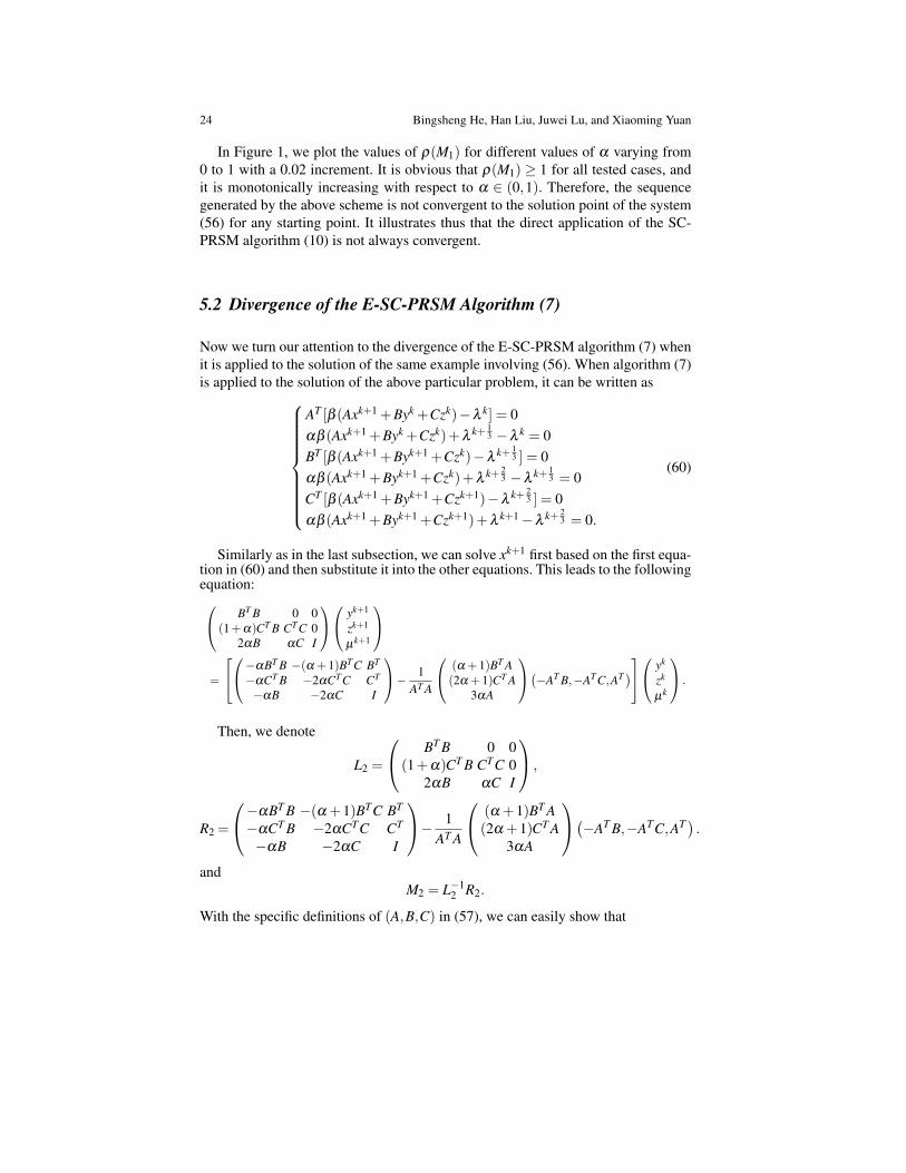
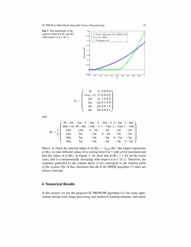


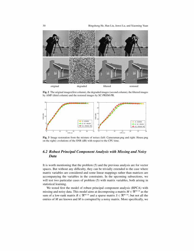


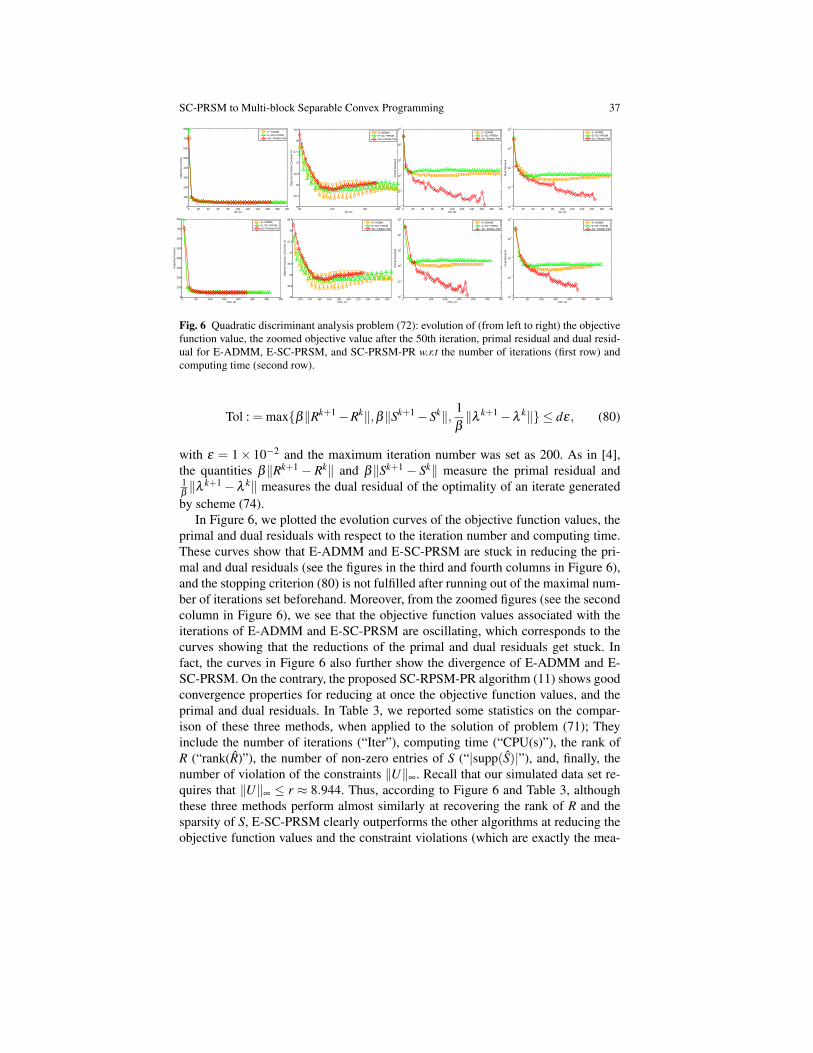


![STRICTLY OBSERVABLE LINEAR SYSETEMSmst.ufl.edu/pdf papers/Strictly observable systems.pdf · 2017. 5. 18. · strictly observable (HAMMER and . HEYMANN [1981b]). We note that a strictly](https://static.documents.pub/doc/80x56/614563f034130627ed50f1f3/strictly-observable-linear-papersstrictly-observable-systemspdf-2017-5-18.jpg)


