Applications of CLP: Robust Optimization - web.stanford.edu · Applications of CLP: Robust...

Conic Linear Optimization and Appl. MS&E314 Lecture Note #15 1

Applications of CLP: Robust Optimization

Yinyu Ye

Department of Management Science and Engineering

Stanford University

Stanford, CA 94305, U.S.A.

http://www.stanford.edu/˜yyye


Standard Optimization Problem

Consider an optimization problem

Minimize f(x, ξ)

(OPT)

subject to F (x, ξ) ∈ K ⊂ Rm.

(1)

where ξ is the data of the problem and x ∈ Rn is the decision vector, and K is

a convex cone.


Data Uncertainty

For deterministic optimization, we assume ξ is known and fixed. In reality, ξ may

not be certain.

• Knowledge of ξ belonging to a given uncertain set U .

• The constraints must be satisfied for every ξ in the uncertain set U .

• Optimal solution must give the best guaranteed value of supξ∈U f(x, ξ).


Stochastic Method

Minimize Eξ[f(x, ξ)]

(EOPT)

subject to Eξ[F (x, ξ)] ∈ K.


Sampling Method

Minimize z

(SOPT)

subject to F (x, ξk) ∈ K

f(x, ξk) ≤ z

for large samples ξk ∈ U.


Robust Counterpart

Minimize supξ∈U f(x, ξ)

(ROPT)

subject to F (x, ξ) ∈ K for all ξ ∈ U.

(2)


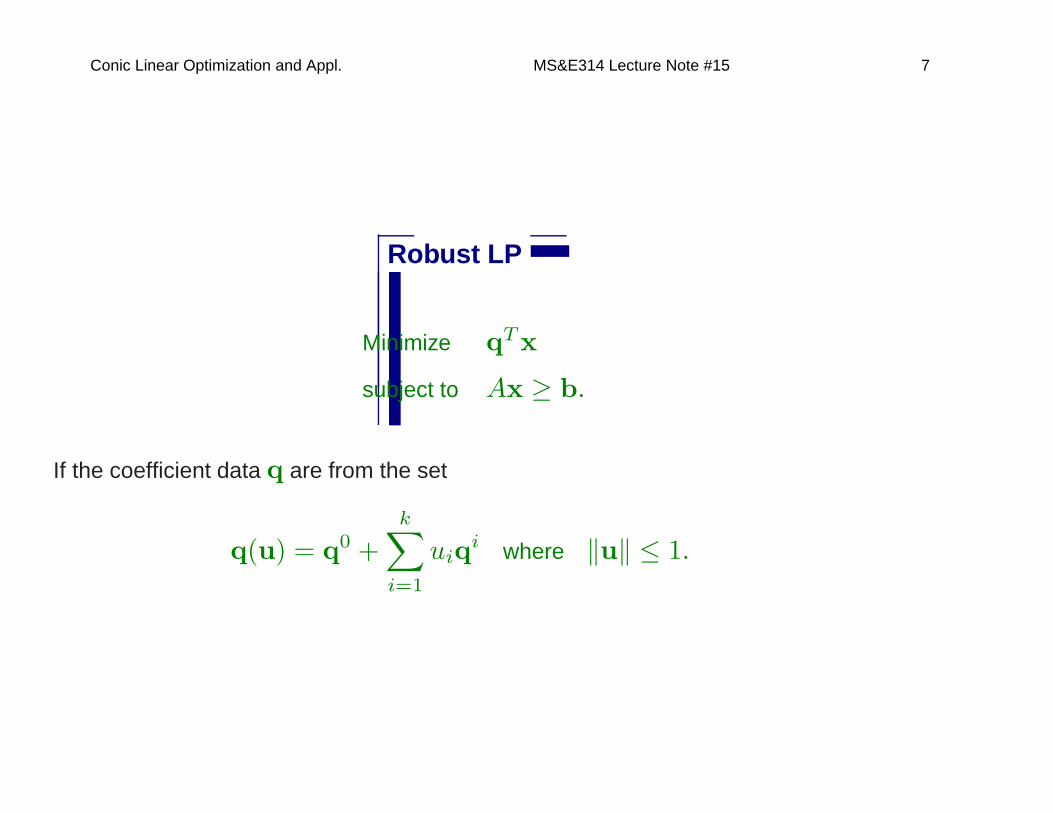
Robust LP

Minimize qTx

subject to Ax ≥ b.

If the coefficient data q are from the set

q(u) = q0 +

k∑i=1

uiqi where ‖u‖ ≤ 1.


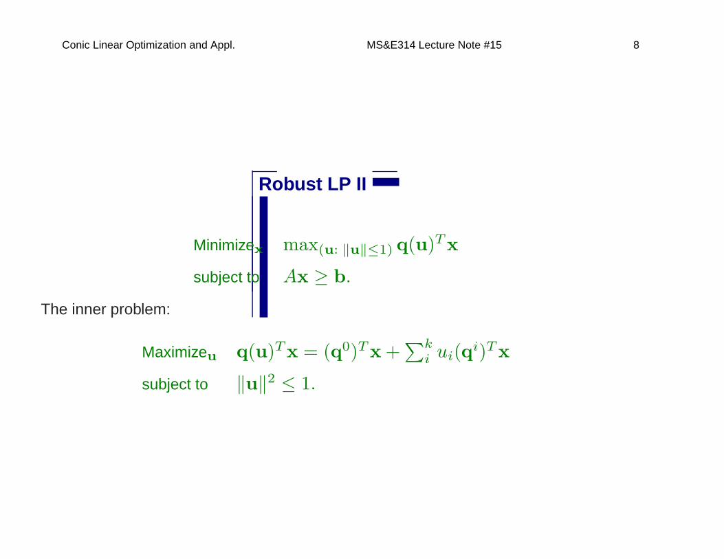
Robust LP II

Minimizex max(u: ‖u‖≤1) q(u)Tx

subject to Ax ≥ b.

The inner problem:

Maximizeu q(u)Tx = (q0)Tx+∑k

i ui(qi)Tx

subject to ‖u‖2 ≤ 1.


Robust LP III

The dual of inner problem:

Minimizeλ (q0)Tx+ λ

subject to λ ≥√∑k

i ((qi)Tx)2.

The integrated SOCP problem:

Minimizex,λ (q0)Tx+ λ

subject to Ax ≥ b,

‖Qx‖ ≤ λ.


Robust Quadratic Optimization

Minimize qTx

(EQP)

subject to ‖Ax‖2 ≤ 1.

(3)

Here, vector q ∈ Rn and A ∈ Rm×n; and ‖.‖ is the Euclidean norm.


2-Norm Uncertainty

A(u) = A0 +

k∑j=1

ujAj where ‖u‖ ≤ 1.

Minimize qTx

(REQP)

subject to ‖(A0 +∑k

j=1 ujAj)x‖2 ≤ 1 ∀‖u‖ ≤ 1.

Let

F (x) = (A0x, A1x, · · · Akx).


Robust Counterpart

‖(A0 +

k∑j=1

ujAj)x‖2 =

⎛⎝ 1

u

⎞⎠

T

F (x)TF (x)

⎛⎝ 1

u

⎞⎠ .

Minimize qTx

(REQP)

subject to

⎛⎝ 1

u

⎞⎠

T ⎛⎝⎛⎝ 1 0

0 0

⎞⎠− F (x)TF (x)

⎞⎠⎛⎝ 1

u

⎞⎠ ≥ 0

∀⎛⎝ 1

u

⎞⎠

T ⎛⎝ 1 0

0 −I

⎞⎠⎛⎝ 1

u

⎞⎠ ≥ 0.


The S-Lemma

Lemma 1 Let P and Q be two symmetric matrices such that there exists u0

satisfying (u0)TPu0 > 0. Then the implication

uTPu ≥ 0 ⇒ uTQu ≥ 0

holds true if and only if there exists λ ≥ 0 such that

Q λP.


Technical Result

⎛⎝ 1

u

⎞⎠

T ⎛⎝⎛⎝ 1 0

0 0

⎞⎠− F (x)TF (x)

⎞⎠⎛⎝ 1

u

⎞⎠ ≥ 0

∀⎛⎝ 1

u

⎞⎠

T ⎛⎝ 1 0

0 −I

⎞⎠⎛⎝ 1

u

⎞⎠ ≥ 0

if and only if there is a λ ≥ 0 such that⎛⎝ 1 0

0 0

⎞⎠− F (x)TF (x) λ

⎛⎝ 1 0

0 −I

⎞⎠ .


The Second Lemma

Lemma 2 Let P a symmetric matrix and A be a rectangle matrix. Then

P −ATA 0

if and only if ⎛⎝ P AT

A I

⎞⎠ 0.


SDP Inequality

⎛⎜⎜⎝⎛⎝ 1 0

0 0

⎞⎠+ λ

⎛⎝ −1 0

0 I

⎞⎠ F (x)T

F (x) I

⎞⎟⎟⎠ 0

which is a SDP constraint since it is linear in x and λ.


SDP Representation

Consider λ and x as variables, REQP finally becomes a SDP problem:

Minimize qTx

(REQP)

subject to

⎛⎜⎜⎝⎛⎝ 1− λ 0

0 λI

⎞⎠ F (x)T

F (x) I

⎞⎟⎟⎠ 0.

This is an SDP problem.


Non-Homogeneous Case

Minimize qTx

(EQP)

subject to −xTATAx+ 2bTx+ γ ≥ 0.

(4)

Here, vector q,b ∈ Rn and and A ∈ Rm×n.


2-Norm Uncertainty

Let A be uncertain and

(A,b, γ) = (A0,b0, γ0) +

k∑j=1

uj(Aj ,bj , γj)| uTu ≤ 1.

Minimize qTx

(REQP)

subject to −xTATAx+ 2bTx+ γ ≥ 0 ∀uTu ≤ 1.

Let again

F (x) = (A0x, A1x, · · · Akx).


Matrix Representation

−xTATAx+ 2bTx+ γ =

(1

u

)T

⎛⎜⎜⎜⎝⎛⎜⎜⎜⎝

γ0 + 2xTb0 γ1/2 + xTb1 · · · γk/2 + xTbk

γ1/2 + xTb1 0 · · · 0

· · · · · · · · · · · ·γk/2 + xTbk 0 · · · 0

⎞⎟⎟⎟⎠− F (x)TF (x)

⎞⎟⎟⎟⎠(

1

u

).


Apply the S-Lemma

If and only if there is λ ≥ 0 such that⎛⎜⎜⎜⎝

γ0 + 2xTb0 γ1/2 + xTb1 · · · γk/2 + xTbk

γ1/2 + xTb1 0 · · · 0

· · · · · · · · · · · ·γk/2 + xTbk 0 · · · 0

⎞⎟⎟⎟⎠− F (x)TF (x))

� λ

(1 0

0 −I

);


SDP Inequality

⎛⎜⎜⎜⎜⎜⎝

⎛⎜⎜⎜⎝

γ0 + 2xTb0 − λ γ1/2 + xTb1 · · · γk/2 + xTbk

γ1/2 + xTb1 λ · · · 0

· · · · · · · · · · · ·γk/2 + xTbk 0 · · · λ

⎞⎟⎟⎟⎠ F (x)T

F (x) I

⎞⎟⎟⎟⎟⎟⎠ � 0.

which is a SDP constraint since the matrix is linear in x and λ.


SDP Representation

Minimize qTx

(REQP)

subject to

⎛⎜⎜⎜⎜⎜⎝

⎛⎜⎜⎜⎝

γ0 + 2xTb0 − λ γ1/2 + xTb1 · · · γk/2 + xTbk

γ1/2 + xTb1 λ · · · 0

· · · · · · · · · · · ·γk/2 + xTbk 0 · · · λ

⎞⎟⎟⎟⎠ F (x)T

F (x) I

⎞⎟⎟⎟⎟⎟⎠ � 0.


General Tool for Robust Quadratic Optimization

Recall

Minimize supξ∈U f(x, ξ)

(ROPT)

subject to F (x, ξ) ≤ 0 for all ξ ∈ U.

(5)


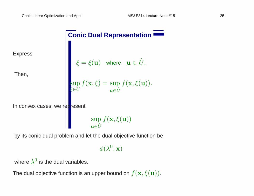
Conic Dual Representation

Express

ξ = ξ(u) where u ∈ U .

Then,

supξ∈U

f(x, ξ) = supu∈U

f(x, ξ(u)).

In convex cases, we represent

supu∈U

f(x, ξ(u))

by its conic dual problem and let the dual objective function be

φ(λ0,x)

where λ0 is the dual variables.

The dual objective function is an upper bound on f(x, ξ(u)).


Robust Counterpart

Minimize φ(λ0,x)

(ROPT)

subject to F (x, ξ(u)) ≤ 0 for all u ∈ U

dual constraints on λ0.

(6)


Conic Constraint Representation

Minimize φ(λ0,x)

(ROPT)

subject to Φ(λ,x) ∈ C

dual constraints on λ0, λ,

(7)

where Φ(λ,x) is, component-wise, the dual objective function of

supu∈U

F (x, ξ(u))

and C is a suitable cone.


Example:

ax+ b ≤ 0

where

(a, b) = (a0, b0) +k∑

i=1

ui(ai, bi)| u ∈ U .


2-Norm Uncertainty

Case of ‖u‖ ≤ 1:

maxu:‖u‖≤1

a0x+ b0 +k∑

i=1

ui(aix+ bi)

which is an SOCP. The dual is

Minimize a0x+ b0 + λ

subject to λ ≥√∑k

i=1(aix+ bi)2.

Thus, the robust constraint becomes

0 ≥ a0x+ b0 + λ ≥ (a0x+ b0) +

√√√√ k∑i=1

(aix+ bi)2.


1-Norm Uncertainty

Case of ‖u‖1 ≤ 1:

maxu:‖u‖1≤1

a0x+ b0 +k∑

i=1

ui(aix+ bi)

which is 1-norm CP. The dual is


subject to λ ≥ maxi{|(aix+ bi)|}.


0 ≥ a0x+ b0 + λ ≥ (a0x+ b0) + maxi

{|(aix+ bi)|}.


∞-Norm Uncertainty

Case of ‖u‖∞ ≤ 1:

maxu:‖u‖∞≤1

a0x+ b0 +

k∑i=1

ui(aix+ bi)

The dual is


subject to λ ≥∑ki=1 |(aix+ bi)|.


0 ≥ a0x+ b0 + λ ≥ (a0x+ b0) +

k∑i=1

|(aix+ bi)|.

Date post:	22-Jul-2019
Category:	Documents
Upload:	vuongkiet
View:	225 times
Download:	0 times

Applications of CLP: Robust Optimization - web.stanford.edu · Applications of CLP: Robust...

Documents