Applications of Convex Analysis within Mathematics - … · Applications of Convex Analysis within...

Noname manuscript No.(will be inserted by the editor)

Applications of Convex Analysis within Mathematics

Francisco J. Aragon Artacho · Jonathan M. Borwein ·Victoria Martın-Marquez · Liangjin Yao

July 19, 2013

Abstract In this paper, we study convex analysis and its theoretical applications. We first apply importanttools of convex analysis to Optimization and to Analysis. We then show various deep applications of convexanalysis and especially infimal convolution in Monotone Operator Theory. Among other things, we recapturethe Minty surjectivity theorem in Hilbert space, and present a new proof of the sum theorem in reflexivespaces. More technically, we also discuss autoconjugate representers for maximally monotone operators.Finally, we consider various other applications in mathematical analysis.

Keywords Adjoint · Asplund averaging · autoconjugate representer · Banach limit · Chebyshev set · convexfunctions · Fenchel duality · Fenchel conjugate · Fitzpatrick function · Hahn–Banach extension theorem ·infimal convolution · linear relation · Minty surjectivity theorem · maximally monotone operator · monotoneoperator ·Moreau’s decomposition ·Moreau envelope ·Moreau’s max formula ·Moreau–Rockafellar duality ·normal cone operator · renorming · resolvent · Sandwich theorem · subdifferential operator · sum theorem ·Yosida approximation

Mathematics Subject Classification (2000) Primary 47N10 · 90C25; Secondary 47H05 · 47A06 ·47B65

Francisco J. Aragon ArtachoCentre for Computer Assisted Research Mathematics and its Applications (CARMA), University of Newcastle, Callaghan, NSW2308, Australia.E-mail: [email protected]

Jonathan M. BorweinCentre for Computer Assisted Research Mathematics and its Applications (CARMA), University of Newcastle, Callaghan, NSW2308, Australia. Laureate Professor at the University of Newcastle and Distinguished Professor at King Abdul-Aziz University,Jeddah.E-mail: [email protected]

Victoria Martın-MarquezDepartamento de Analisis Matematico, Facultad de Matematicas, Universidad de Sevilla, PO Box 1160, 41080 Sevilla, Spain.E-mail: [email protected]

Liangjin YaoCentre for Computer Assisted Research Mathematics and its Applications (CARMA), University of Newcastle, Callaghan, NSW2308, Australia.E-mail: [email protected]

2 Francisco J. Aragon Artacho et al.

1 Introduction

While other articles in this collection look at the applications of Moreau’s seminal work, we have optedto illustrate the power of his ideas theoretically within optimization theory and within mathematics moregenerally. Space constraints preclude being comprehensive, but we think the presentation made shows howelegantly much of modern analysis can be presented thanks to the work of Jean-Jacques Moreau and others.

1.1 Preliminaries

Let X be a real Banach space with norm ‖ · ‖ and dual norm ‖ · ‖∗. When there is no ambiguity we suppressthe ∗. We write X∗ and 〈 · , · 〉 for the real dual space of continuous linear functions and the duality paring,respectively, and denote the closed unit ball by BX := {x ∈ X | ‖x‖ ≤ 1} and set N := {1, 2, 3, . . .}. Weidentify X with its canonical image in the bidual space X∗∗. A set C ⊆ X is said to be convex if it containsall line segments between its members: λx+ (1− λ)y ∈ C whenever x, y ∈ C and 0 ≤ λ ≤ 1.

Given a subset C of X, intC is the interior of C and C is the norm closure of C. For a set D ⊆ X∗, Dw*

is the weak∗ closure of D. The indicator function of C, written as ιC , is defined at x ∈ X by

ιC(x) :=

{0, if x ∈ C;

+∞, otherwise.(1)

The support function of C, written as σC , is defined by σC(x∗) := supc∈C〈c, x∗〉. There is also a naturallyassociated (metric) distance function, that is,

dC(x) := inf {‖x− y‖ | y ∈ C} . (2)

Distance functions play a central role in convex analysis, both theoretically and algorithmically.Let f : X → ]−∞,+∞] be a function. Then dom f := f−1(R) is the domain of f , and the lower level

sets of a function f : X → ]−∞,+∞] are the sets {x ∈ X | f(x) ≤ α} where α ∈ R. The epigraph of fis epi f := {(x, r) ∈ X × R | f(x) ≤ r}. We will denote the set of points of continuity of f by cont f . Thefunction f is said to be convex if for any x, y ∈ dom f and any λ ∈ [0, 1], one has

f(λx+ (1− λ)y) ≤ λf(x) + (1− λ)f(y).

We say f is proper if dom f 6= ∅. Let f be proper. The subdifferential of f is defined by

∂f : X ⇒ X∗ : x 7→ {x∗ ∈ X∗ | 〈x∗, y − x〉 ≤ f(y)− f(x), for all y ∈ X}.

By the definition of ∂f , even when x ∈ dom f , it is possible that ∂f(x) may be empty. For example ∂f(0) = ∅for f(x) := −

√x whenever x ≥ 0 and f(x) := +∞ otherwise. If x∗ ∈ ∂f(x) then x∗ is said to be a subgradient

of f at x. An important example of a subdifferential is the normal cone to a convex set C ⊆ X at a pointx ∈ C which is defined as NC(x) := ∂ιC(x).

Let g : X → ]−∞,+∞]. Then the inf-convolution f�g is the function defined on X by

f�g : x 7→ infy∈X

{f(y) + g(x− y)

}.

(In [45] Moreau studied inf-convolution when X is an arbitrary commutative semigroup.) Notice that, ifboth f and g are convex, so it is f�g (see, e.g., [49, p. 17]).

We use the convention that (+∞) + (−∞) = +∞ and (+∞) − (+∞) = +∞. We will say a functionf : X → ]−∞,+∞] is Lipschitz on a subset D of dom f if there is a constant M ≥ 0 so that |f(x)− f(y)| ≤M‖x− y‖ for all x, y ∈ D. In this case M is said to be a Lipschitz constant for f on D. If for each x0 ∈ D,there is an open set U ⊆ D with x0 ∈ U and a constant M so that |f(x) − f(y)| ≤ M‖x − y‖ for all

Applications of Convex Analysis within Mathematics 3

x, y ∈ U , we will say f is locally Lipschitz on D. If D is the entire space, we simply say f is Lipschitz orlocally Lipschitz respectively.

Consider a function f : X → ]−∞,+∞]; we say f is lower-semicontinuous (lsc) if lim infx→x f(x) ≥ f(x)for all x ∈ X, or equivalently, if epi f is closed. The function f is said to be sequentially weakly lowersemi-continuous if for every x ∈ X and every sequence (xn)n∈N which is weakly convergent to x, one haslim infn→∞ f(xn) ≥ f(x). This is a useful distinction since there are infinite dimensional Banach spaces(Schur spaces such as `1) in which weak and norm convergence coincide for sequences, see [22, p. 384, esp.Thm 8.2.5].

1.2 Structure of this paper

The remainder of this paper is organized as follows. In Section 2, we describe results about Fenchel conjugatesand the subdifferential operator, such as Fenchel duality, the Sandwich theorem, etc. We also look at someinteresting convex functions and inequalities. In Section 3, we discuss the Chebyshev problem from abstractapproximation. In Section 4, we show applications of convex analysis in Monotone Operator Theory. Wereprise such results as the Minty surjectivity theorem, and present a new proof of the sum theorem inreflexive spaces. We also discuss Fitzpatrick’s problem on so called autoconjugate representers for maximallymonotone operators. In Section 5 we discuss various other applications.

2 Subdifferential operators, conjugate functions & Fenchel duality

We begin with some fundamental properties of convex sets and convex functions. While many results holdin all locally convex spaces, some of the most important such as (iv)(b) in the next Fact do not.

Fact 1 (Basic properties [22, Ch. 2 and 4].) The following hold.

(i) The (lsc) convex functions form a convex cone closed under pointwise suprema: if fγ is convex (and lsc)for each γ ∈ Γ then so is x 7→ supγ∈Γ fγ(x).

(ii) A function f is convex if and only if epi f is convex if and only if ιepi f is convex.(iii) Global minima and local minima in the domain coincide for proper convex functions.(iv) Let f be a proper convex function and let x ∈ dom f . (a) f is locally Lipschitz at x if and only f is

continuous at x if and only if f is locally bounded at x. (b) Additionally, if f is lower semicontinuous,then f is continuous at every point in int dom f .

(v) A proper lower semicontinuous and convex function is bounded from below by a continuous affine function.(vi) If C is a nonempty set, then dC(·) is non-expansive (i.e., is a Lipschitz function with constant one).

Additionally, if C is convex, then dC(·) is a convex function.(vii) If C is a convex set, then C is weakly closed if and only if it is norm closed.(viii) Three-slope inequality: Suppose f : R→]−∞,∞] is convex and a < b < c. Then

f(b)− f(a)

b− a≤ f(c)− f(a)

c− a≤ f(c)− f(b)

c− b.

The following trivial fact shows the fundamental significance of subgradients in optimization.

Proposition 1 (Subdifferential at optimality) Let f : X → ]−∞,+∞] be a proper convex function.Then the point x ∈ dom f is a (global) minimizer of f if and only if 0 ∈ ∂f(x).

The directional derivative of f at x ∈ dom f in the direction d is defined by

f ′(x; d) := limt→0+

f(x+ td)− f(x)

t


if the limit exists. If f is convex, the directional derivative is everywhere finite at any point of int dom f , andit turns out to be Lipschitz at cont f . We use the term directional derivative with the understanding that itis actually a one-sided directional derivative.

If the directional derivative f ′(x, d) exists for all directions d and the operator f ′(x) defined by 〈f ′(x), · 〉 :=f ′(x; · ) is linear and bounded, then we say that f is Gateaux differentiable at x, and f ′(x) is called theGateaux derivative. Every function f : X → ]−∞,+∞] which is lower semicontinuous, convex and Gateauxdifferentiable at x, it is continuous at x. Additionally, the following properties are relevant for the existenceand uniqueness of the subgradients.

Proposition 2 (See [22, Fact 4.2.4 and Corollary 4.2.5].) Suppose f : X → ]−∞,+∞] is convex.

(i) If f is Gateaux differentiable at x, then f ′(x) ∈ ∂f(x).(ii) If f is continuous at x, then f is Gateaux differentiable at x if and only if ∂f(x) is a singleton.

Example 1 We show that part (ii) in Proposition 2 is not always true in infinite dimensions without continuityhypotheses.

(a) The indicator of the Hilbert cube C := {x = (x1, x2, . . .) ∈ `2 : |xn| ≤ 1/n,∀n ∈ N} at zero or any othernon-support point has a unique subgradient but is nowhere Gateaux differentiable.

(b) Boltzmann-Shannon entropy x 7→∫ 1

0x(t) log(x(t))dt viewed as a lower semicontinuous and convex func-

tion on L1[0, 1] has unique subgradients at x(t) > 0 a.e. but is nowhere Gateaux differentiable (which fora lower semicontinuous and convex function in Banach space implies continuity).

That Gateaux differentiability of a convex and lower semicontinuous function implies continuity at the pointis a consequence of the Baire category theorem. ♦

The next result proved by Moreau in 1963 establishes the relationship between subgradients and directionalderivatives, see also [49, page 65]. Proofs can be also found in most of the books in variational analysis, seee.g. [25, Theorem 4.2.7].

Theorem 1 (Moreau’s max formula [46]) Let f : X → ]−∞,+∞] be a convex function and let d ∈ X.Suppose that f is continuous at x. Then, ∂f(x) 6= ∅ and

f ′(x; d) = max{〈x∗, d〉 | x∗ ∈ ∂f(x)}. (3)

Let f : X → [−∞,+∞]. The Fenchel conjugate (also called the Legendre-Fenchel conjugate1 or transform)of f is the function f∗ : X∗ → [−∞,+∞] defined by

f∗(x∗) := supx∈X{〈x∗, x〉 − f(x)}.

We can also consider the conjugate of f∗ called the biconjugate of f and denoted by f∗∗. This is a convexfunction on X∗∗ satisfying f∗∗|X ≤ f . A useful and instructive example is σC = ι∗C .

Example 2 Let 1 < p < ∞ . If f(x) := ‖x‖pp for x ∈ X then f∗(x∗) =

‖x∗‖q∗q , where 1

p + 1q = 1. Indeed, for

any x∗ ∈ X∗, one has

f∗(x∗) = supλ∈R+

sup‖x‖=1

{〈x∗, λx〉 − ‖λx‖

p

p

}= supλ∈R+

{λ‖x∗‖∗ −

λp

p

}=‖x∗‖q∗q

.

♦

1 Originally the connection was made between a monotone function on an interval and its inverse. The convex functions thenarise by integration.


By direct construction and Fact 1 (i), for any function f , the conjugate function f∗ is always convexand lower semicontinuous, and if the domain of f is nonempty, then f∗ never takes the value −∞. Theconjugate plays a role in convex analysis in many ways analogous to the role played by the Fourier transformin harmonic analysis with infimal convolution, see below, replacing integral convolution and sum replacingproduct [22, Chapter 2.].

2.1 Inequalities and their applications

An immediate consequence of the definition is that for f, g : X → [−∞,+∞], the inequality f ≥ g impliesf∗ ≤ g∗. An important result which is straightforward to prove is the following.

Proposition 3 (Fenchel–Young) Let f : X → ]−∞,+∞]. All points x∗ ∈ X∗ and x ∈ dom f satisfy theinequality

f(x) + f∗(x∗) ≥ 〈x∗, x〉. (4)

Equality holds if and only if x∗ ∈ ∂f(x).

Example 3 (Young’s inequality) By taking f as in Example 2, one obtains directly from Proposition 3

‖x‖p

p+‖x∗‖q∗q≥ 〈x∗, x〉,

for all x ∈ X and x∗ ∈ X∗, where p > 1 and 1p + 1

q = 1. When X = R one recovers the original Younginequality. ♦

This in turn leads to one of the workhorses of modern analysis:

Example 4 (Holder’s inequality) Let f and g be measurable on a measure space (X,µ). Then∫X

fg dµ ≤ ‖f‖p‖g‖q, (5)

where 1 < p < ∞ and 1p + 1

q = 1. Indeed, by rescaling, we may assume without loss of generality that

‖f‖p = ‖g‖q = 1. Then Young’s inequality in Example 3 yields

|f(x)g(x)| ≤ |f(x)|p

p+|g(x)|q

qfor x ∈ X,

and (5) follows by integrating both sides. The result holds true in the limit for p = 1 or p =∞. ♦

We next take a brief excursion into special function theory and normed space geometry to emphasize that“convex functions are everywhere.”

Example 5 (Bohr–Mollerup theorem) The Gamma function defined for x > 0 as

Γ (x) :=

∫ ∞0

e−ttx−1dt = limn→∞

n!nx

x(x+ 1) · · · (x+ n)

is the unique function f mapping the positive half-line to itself and such that (a) f(1) = 1, (b) xf(x) =f(x+ 1) and (c) log f is a convex function.

Indeed, clearly Γ (1) = 1, and it is easy to prove (b) for Γ by using integration by parts. In order to showthat logΓ is convex, pick any x, y > 0 and λ ∈ (0, 1) and apply Holder’s inequality (5) with p = 1/λ to thefunctions t 7→ e−λttλ(x−1) and t 7→ e−(1−λ)tt(1−λ)(y−1). For the converse, let g := log f . Then (a) and (b)


imply g(n+ 1 + x) = log [x(1 + x) . . . (n+ x)f(x)] and thus g(n+ 1) = log(n!). Convexity of g together withthe three-slope inequality, see Fact 1(viii), implies that

g(n+ 1)− g(n) ≤ g(n+ 1 + x)− g(n+ 1)

x≤ g(n+ 2 + x)− g(n+ 1 + x),

and hence,x log(n) ≤ log (x(x+ 1) · · · (x+ n)f(x))− log(n!) ≤ x log(n+ 1 + x);

whence,

0 ≤ g(x)− log

(n!nx

x(x+ 1) · · · (x+ n)

)≤ x log

(1 +

1 + x

n

).

Taking limits when n→∞ we obtain

f(x) = limn→∞

n!nx

x(x+ 1) · · · (x+ n)= Γ (x).

As a bonus we recover a classical and important limit formula for Γ (x).Application of the Bohr–Mollerup theorem is often automatable in a computer algebra system, as we now

illustrate. Consider the beta function

β(x, y) :=

∫ 1

0

tx−1(1− t)y−1 d t (6)

for Re(x),Re(y) > 0. As is often established using polar coordinates and double integrals

β(x, y) =Γ (x)Γ (y)

Γ (x+ y). (7)

We may use the Bohr–Mollerup theorem with

f := x→ β(x, y)Γ (x+ y)/Γ (y)

to prove (7) for real x, y.Now (a) and (b) from Example 5 are easy to verify. For (c) we again use Holder’s inequality to show f is

log-convex. Thus, f = Γ as required. ♦

Example 6 (Blaschke–Santalo theorem) The volume of a unit ball in the ‖ · ‖p-norm, Vn(p) is

Vn(p) = 2nΓ (1 + 1

p )n

Γ (1 + np )

. (8)

as was first determined by Dirichlet. When p = 2, this gives

Vn = 2nΓ ( 3

2 )n

Γ (1 + n2 )

=Γ ( 1

2 )n

Γ (1 + n2 ),

which is more concise than that usually recorded in texts.Let C in Rn be a convex body which is symmetric around zero, that is, a closed bounded convex set with

nonempty interior. Denoting n-dimensional Euclidean volume of S ⊆ Rn by Vn(S), the Blaschke–Santaloinequality says

Vn(C)Vn(C◦) ≤ Vn(E)Vn(E◦) = V 2n (Bn(2)) (9)

where maximality holds (only) for any symmetric ellipsoid E and Bn(2) is the Euclidean unit ball. It isconjectured the minimum is attained by the 1-ball and the ∞-ball. Here as always the polar set is definedby C◦ := {y ∈ Rn : 〈y, x〉 ≤ 1 for all x ∈ C}.

The p-ball case of (9) follows by proving the following convexity result:


Theorem 2 (Harmonic-arithmetic log-concavity) The function

Vα(p) := 2αΓ

(1 +

1

p

)α/Γ

(1 +

α

p

)satisfies

Vα(p)λ Vα(q)1−λ < Vα

(1

λp + 1−λ

q

), (10)

for all α > 1, if p, q > 1, p 6= q, and λ ∈ (0, 1).

Set α := n, 1p + 1

q = 1 with λ = 1−λ = 1/2 to recover the p−norm case of the Blaschke–Santalo inequality. Itis amusing to deduce the corresponding lower bound. This technique extends to various substitution norms.Further details may be found in [16, §5.5]. Note that we may easily explore Vα(p) graphically. ♦

2.2 The biconjugate and duality

The next result has been associated by different authors with the names of Legendre, Fenchel, Moreau andHormander; see, e.g., [22, Proposition 4.4.2].

Proposition 4 (Hormander2) (See [66, Theorem 2.3.3] or [22, Proposition 4.4.2(a)].) Let f : X →]−∞,+∞] be a proper function. Then

f is convex and lower semicontinuous ⇔ f = f∗∗|X .

Example 7 (Establishing convexity) (See [12, Theorem 1].) We may compute conjugates by hand or using thesoftware SCAT [20]. This is discussed further in Section 5.3. Consider f(x) := ex. Then f∗(x) = x log(x)−xfor x ≥ 0 (taken to be zero at zero) and is infinite for x < 0. This establishes the convexity of x log(x) − xin a way that takes no knowledge of x log(x).

A more challenging case is the following (slightly corrected) conjugation formula [21, p. 94, Ex. 13] whichcan be computed algorithmically: Given real α1, α2, . . . , αm > 0, define α :=

∑i αi and suppose a real µ

satisfies µ > α+ 1. Now define a function f : Rm × R 7→ ]−∞,+∞] by

f(x, s) :=

µ−1sµ

∏i x−αii if x ∈ Rm++, s ∈ R+;

0 if ∃xi = 0, x ∈ Rm+ , s = 0;

+∞ otherwise.

, ∀x := (xn)mn=1 ∈ Rm, s ∈ R.

It transpires that

f∗(y, t) =

ρν−1tν

∏i(−yi)−βi if y ∈ Rm−−, t ∈ R+

0 if y ∈ Rm− , t ∈ R−+∞ otherwise

, ∀y := (yn)mn=1 ∈ Rm, t ∈ R.

for constants

ν :=µ

µ− (α+ 1), βi :=

αiµ− (α+ 1)

, ρ :=∏i

(αiµ

)βi.

We deduce that f = f∗∗, whence f (and f∗) is (essentially strictly) convex. For attractive alternative proofof convexity see [42]. Many other substantive examples are to be found in [21,22]. ♦

2 Hormander first proved the case of support and indicator functions in [38] which led to discovery of general result.


The next theorem gives us a remarkable sufficient condition for convexity of functions in terms of theGateaux differentiability of the conjugate. There is a simpler analogue for the Frechet derivative.

Theorem 3 (See [22, Corollary 4.5.2].) Suppose f : X → ]−∞,+∞] is such that f∗∗ is proper. If f∗ isGateaux differentiable at all x∗ ∈ dom ∂f∗ and f is sequentially weakly lower semicontinuous, then f isconvex.

Let f : X → ]−∞,+∞]. We say f is coercive if lim‖x‖→∞ f(x) = +∞. We say f is supercoercive if

lim‖x‖→∞f(x)‖x‖ = +∞.

Fact 2 (See [22, Fact 4.4.8].) If f is proper convex and lower semicontinuous at some point in its domain,then the following statements are equivalent.

(i) f is coercive.(ii) There exist α > 0 and β ∈ R such that f ≥ α‖ · ‖+ β.(iii) lim inf‖x‖→∞ f(x)/‖x‖ > 0.(iv) f has bounded lower level sets.

Because a convex function is continuous at a point if and only if it is bounded above on a neighborhoodof that point (Fact 1(iv)), we get the following result; see also [38, Theorem 7] for the case of the indicatorfunction of a bounded convex set.

Theorem 4 (Hormander–Moreau–Rockafellar) Let f : X → ]−∞,+∞] be convex and lower semicon-tinuous at some point in its domain, and let x∗ ∈ X∗. Then f −x∗ is coercive if and only if f∗ is continuousat x∗.

Proof. “⇒”: By Fact 2, there exist α > 0 and β ∈ R such that f ≥ x∗+α‖·‖+β. Then f∗ ≤ −β+ι{x∗+αBX∗},from where x∗ + αBX∗ ⊆ dom f∗. Therefore, f∗ is continuous at x∗ by Fact 1(iv).

“⇐”: By the assumption, there exists β ∈ R and δ > 0 such that

f∗(x∗ + z∗) ≤ β, ∀z∗ ∈ δBX∗ .

Thus, by Proposition 3,〈x∗ + z∗, y〉 − f(y) ≤ β, ∀z∗ ∈ δBX∗ , ∀y ∈ X;

whence, taking the supremum with z∗ ∈ δBX∗ ,

δ‖y‖ − β ≤ f(y)− 〈x∗, y〉, ∀y ∈ X.

Then, by Fact 2, f − x∗ is coercive. �

Example 8 Given a set C in X, recall that the negative polar cone of C is the convex cone

C− := {x∗ ∈ X∗ | sup〈x∗, C〉 ≤ 0}.

Suppose that X is reflexive and let K ⊆ X be a closed convex cone. Then K− is another nonempty closedconvex cone with K−− := (K−)− = K. Moreover, the indicator function of K and K− are conjugate toeach other. If we set f := ιK− , the indicator function of the negative polar cone of K, Theorem 4 applies toget that

x ∈ intK if and only if the set {x∗ ∈ K− | 〈x∗, x〉 ≥ α} is bounded for any α ∈ R.

Indeed, since x ∈ intK = int dom ι∗K− if and only if ι∗K− is continuous at x, from Theorem 4 we have that thisis true if and only if the function ιK− − x is coercive. Now, Fact 2 assures us that coerciveness is equivalentto boundedness of the lower level sets, which implies the assertion. ♦


Theorem 5 (Moreau–Rockafellar duality [47]) Let f : X → (−∞,+∞] be a lower semicontinuousconvex function. Then f is continuous at 0 if and only if f∗ has weak∗-compact lower level sets.

Proof. Observe that f is continuous at 0 if and only if f∗∗ is continuous at 0 ([22, Fact 4.4.4(b)])if and onlyif f∗ is coercive (Theorem 4) if and only if f∗ has bounded lower level sets (Fact 2) if and only if f∗ hasweak∗-compact lower level sets by the Banach-Alaoglu theorem (see [59, Theorem 3.15]). �

Theorem 6 (Conjugates of supercoercive functions) Suppose f : X → ]−∞,+∞] is a lower semi-continuous and proper convex function. Then

(a) f is supercoercive if and only if f∗ is bounded (above) on bounded sets.(b) f is bounded (above) on bounded sets if and only if f∗ is supercoercive.

Proof. (a) “⇒”: Given any α > 0, there exists M such that f(x) ≥ α‖x‖ if ‖x‖ ≥M . Now there exists β ≥ 0such that f(x) ≥ −β if ‖x‖ ≤ M by Fact 1(v). Therefore f ≥ α‖ · ‖ + (−αM − β). Thus, it implies thatf∗ ≤ α(‖ · ‖)∗( ·α ) + αM + β and hence f∗ ≤ αM + β on αBX∗ .

“⇐”: Let γ > 0. Now there exists K such that f∗ ≤ K on γBX∗ . Then f ≥ γ‖ · ‖ − K and so

lim inf‖x‖→∞f(x)‖x‖ ≥ γ. Hence lim inf‖x‖→∞

f(x)‖x‖ = +∞.

(b): According to (a), f∗ is supercoercive if and only if f∗∗ is bounded on bounded sets. By [22,Fact 4.4.4(a)] this holds if and only if f is bounded (above) on bounded sets. �

We finish this subsection by recalling some properties of infimal convolutions. Some of their many ap-plications include smoothing techniques and approximation. We shall meet them again in Section 4. Letf, g : X → ]−∞,+∞]. Geometrically, the infimal convolution of f and g is the largest extended real-valuedfunction whose epigraph contains the sum of epigraphs of f and g (see example in Figure 1), consequentlyit is a convex function. The following is a useful result concerning the conjugate of the infimal convolution.

Fact 3 (See [22, Lemma 4.4.15] and [49, pp. 37-38].) If f and g are proper functions on X, then (f�g)∗ =f∗+ g∗. Additionally, suppose f, g are convex and bounded below. If f : X → R is continuous (resp. boundedon bounded sets, Lipschitz), then f�g is a convex function that is continuous (resp. bounded on boundedsets, Lipschitz).

Remark 1 Suppose C is a nonempty convex set. Then dC = ‖ · ‖�ιC , implying that dC is a Lipschitz convexfunction. ♦

Example 9 Consider f, g : R→ ]−∞,+∞] given by

f(x) :=

{−√

1− x2, for − 1 ≤ x ≤ 1,+∞ otherwise,

and g(x) := |x|.

The infimal convolution of f and g is

(f�g)(x) =

{−√

1− x2, −√

22 ≤ x ≤ −

√2

2 ;

|x| −√

2, otherwise.,

as shown in Figure 1. ♦


-1.5 -1 -0.5 0.5 1 1.5

-1

-0.5

0.5

1

1.5

g

ff g•

(f+g)epi

Fig. 1 Infimal convolution of f(x) = −√

1− x2 and g(x) = |x|.

2.3 The Hahn-Banach circle

Let T : X → Y be a linear mapping between two Banach spaces X and Y . The adjoint of T is the linearmapping T ∗ : Y ∗ → X∗ defined, for y∗ ∈ Y ∗, by

〈T ∗y∗, x〉 = 〈y∗, Tx〉 for all x ∈ X.

A flexible modern version of Fenchel’s celebrated duality theorem is:

Theorem 7 (Fenchel duality) Let Y be another Banach space, let f : X → ]−∞,+∞] and g : Y →]−∞,+∞] be convex functions and let T : X → Y be a bounded linear operator. Define the primal and dualvalues p, d ∈ [−∞,+∞] by solving the Fenchel problems

p := infx∈X{f(x) + g(Tx)}

d := supy∗∈Y ∗

{−f∗(T ∗y∗)− g∗(−y∗)}. (11)

Then these values satisfy the weak duality inequality p ≥ d.Suppose further that f , g and T satisfy either⋃

λ>0

λ [dom g − T dom f ] = Y and both f and g are lower semicontinuous, (12)

or the conditioncont g ∩ T dom f 6= ∅. (13)

Then p = d, and the supremum in the dual problem (11) is attained when finite. Moreover, the perturbationfunction h(u) := infx f(x) + g(Tx+ u) is convex and continuous at zero.

Generalizations of Fenchel duality Theorem can be found in [27,26]. An easy consequence is:

Corollary 1 (Infimal convolution) Under the hypotheses of the Fenchel duality theorem 7 (f +g)∗(x∗) =(f∗�g∗)(x∗) with attainment when finite.


Another nice consequence of Fenchel duality is the ability to obtain primal solutions from dual ones, aswe now record.

Corollary 2 Suppose the conditions for equality in the Fenchel duality Theorem 7 hold, and that y∗ ∈ Y ∗is an optimal dual solution. Then the point x ∈ X is optimal for the primal problem if and only if it satisfiesthe two conditions T ∗y∗ ∈ ∂f(x) and −y∗ ∈ ∂g(T x).

The regularity conditions in Fenchel duality theorem can be weakened when each function is polyhedral,i.e., when their epigraph is polyhedral.

Theorem 8 (Polyhedral Fenchel duality) (See [21, Corollary 5.1.9].) Suppose that X is a finite-dimensional space. The conclusions of the Fenchel duality Theorem 7 remain valid if the regularity con-dition (12) is replaced by the assumption that the functions f and g are polyhedral with

dom g ∩ T dom f 6= ∅.

Fenchel duality applied to a linear programming program yields the well-known Lagrangian duality.

Corollary 3 (Linear programming duality) Given c ∈ Rn, b ∈ Rm and A an m × n real matrix, onehas

infx∈Rn{cTx | Ax ≤ b} ≥ sup

λ∈Rm+{−bTλ | ATλ = −c}, (14)

where Rm+ :={

(x1, x2, · · · , xm) | xi ≥ 0, i = 1, 2, · · · ,m}

. Equality in (14) holds if b ∈ ranA+Rm+ . Moreover,both extrema are obtained when finite.Proof. Take f(x) := cTx, T := A and g(y) := ιb≥(y) where b≥ := {y ∈ Rm | y ≤ b}. Then apply thepolyhedral Fenchel duality Theorem 8 observing that f∗ = ι{c}, and for any λ ∈ Rm,

g∗(λ) = supy≤b

yTλ =

{bTλ, if λ ∈ Rm+ ;+∞, otherwise;

and (14) follows, since dom g ∩A dom f = {Ax ∈ Rm | Ax ≤ b}. �One can easily derive various relevant results from Fenchel duality, such as the Sandwich theorem, the

subdifferential sum rule, and the Hahn-Banach extension theorem, among many others.

Theorem 9 (Extended sandwich theorem) Let X and Y be Banach spaces and let T : X → Y be abounded linear mapping. Suppose that f : X → ]−∞,+∞], g : Y → ]−∞,+∞] are proper convex functionswhich together with T satisfy either (12) or (13). Assume that f ≥ −g ◦ T . Then there is an affine functionα : X → R of the form α(x) = 〈T ∗y∗, x〉 + r satisfying f ≥ α ≥ −g ◦ T . Moreover, for any x satisfyingf(x) = (−g ◦ T )(x), we have −y∗ ∈ ∂g(T x).

Proof. With notation as in the Fenchel duality Theorem 7, we know d = p, and since p ≥ 0 becausef(x) ≥ −g(Tx), the supremum in d is attained. Therefore there exists y∗ ∈ Y ∗ such that

0 ≤ p = d = −f∗(T ∗y∗)− g∗(−y∗).

Then, by Fenchel-Young inequality (4), we obtain

0 ≤ p ≤ f(x)− 〈T ∗y∗, x〉+ g(y) + 〈y∗, y〉, (15)

for any x ∈ X and y ∈ Y . For any z ∈ X, setting y = Tz in the previous inequality, we obtain

a := supz∈X

[−g(Tz)− 〈T ∗y∗, z〉] ≤ b := infx∈X

[f(x)− 〈T ∗y∗, x〉]

Now choose r ∈ [a, b]. The affine function α(x) := 〈T ∗y∗, x〉+ r satisfies f ≥ α ≥ −g ◦ T , as claimed.


The last assertion follows from (15) simply by setting x = x, where x satisfies f(x) = (−g ◦ T )(x). Thenwe have supy∈Y {〈−y∗, y〉 − g(y)} ≤ (−g ◦ T )(x)− 〈T ∗y∗, x〉. Thus g∗(−y∗) + g(T x) ≤ −〈y∗, T x〉 and hence−y∗ ∈ ∂g(T x). �

When X = Y and T is the identity we recover the classical Sandwich theorem. The next example showsthat without a constraint qualification, the sandwich theorem may fail.

Example 10 Consider f, g : R→ ]−∞,+∞] given by

f(x) :=

{−√−x, for x ≤ 0,

+∞ otherwise,and g(x) :=

{−√x, for x ≥ 0,

+∞ otherwise.

In this case,⋃λ>0 λ [dom g − dom f ] = [0,+∞[ 6= R and it is not difficult to prove there is not any affine

function which separates f and −g, see Figure 2. ♦

The prior constraint qualifications are sufficient but not necessary for the sandwich theorem as we illustratein the next example.

Example 11 Let f, g : R→ ]−∞,+∞] be given by

f(x) :=

{1x , for x > 0,+∞ otherwise,

and g(x) :=

{− 1x , for x < 0,

+∞ otherwise.

Despite that⋃λ>0 λ [dom g − dom f ] = ]−∞, 0[ 6= R, the affine function α(x) := −x satisfies f ≥ α ≥ −g,

see Figure 2. ♦

f

−g f

−g

Fig. 2 On the left we show the failure of the sandwich theorem in the absence of the constraint qualification; of the right weshow that the constraint qualification is not necessary.

Theorem 10 (Subdifferential sum rule) Let X and Y be Banach spaces, and let f : X → ]−∞,+∞]and g : Y → ]−∞,+∞] be convex functions and let T : X → Y be a bounded linear mapping. Then at anypoint x ∈ X we have the sum rule

∂(f + g ◦ T )(x) ⊇ ∂f(x) + T ∗(∂g(Tx))

with equality if (12) or (13) hold.


Proof. The inclusion is straightforward by using the definition of the subdifferential, so we prove the reverseinclusion. Fix any x ∈ X and let x∗ ∈ ∂(f + g ◦T )(x). Then 0 ∈ ∂(f −〈x∗, · 〉+ g ◦T )(x). Conditions for theequality in Theorem 7 are satisfied for the functions f(·) − 〈x∗, · 〉 and g. Thus, there exists y∗ ∈ Y ∗ suchthat

f(x)− 〈x∗, x〉+ g(Tx) = −f∗(T ∗y∗ + x∗)− g∗(−y∗).

Now set z∗ := T ∗y∗ + x∗. Hence, by the Fenchel-Young inequality (4), one has

0 ≤ f(x) + f∗(z∗)− 〈z∗, x〉 = −g(Tx)− g∗(−y∗)− 〈T ∗y∗, x〉 ≤ 0;

whence,

f(x) + f∗(z∗) = 〈z∗, x〉g(Tx) + g∗(−y∗) = 〈−y∗, Tx〉.

Therefore equality in Fenchel-Young occurs, and one has z∗ ∈ ∂f(x) and −y∗ ∈ ∂g(Tx), which completesthe proof. �

The subdifferential sum rule for two convex functions with a finite common point where one of themis continuous was proved by Rockafellar in 1966 with an argumentation based on Fenchel duality, see [55,Th. 3]. In an earlier work in 1963, Moreau [46] proved the subdifferential sum rule for a pair of convex andlsc functions, in the case that infimal convolution of the conjugate functions is achieved, see [49, p. 63] formore details. Moreau actually proved this result for functions which are the supremum of a family of affinecontinuous linear functions, a set which agrees with the convex and lsc functions when X is a locally convexvector space, see [44] or [49, p. 28]. See also [36,37,27,19] for more information about the subdifferentialcalculus rule.

Theorem 11 (Hahn–Banach extension) Let X be a Banach space and let f : X → R be a continuoussublinear function with dom f = X. Suppose that L is a linear subspace of X and the function h : L→ R islinear and dominated by f , that is, f ≥ h on L. Then there exists x∗ ∈ X∗, dominated by f , such that

h(x) = 〈x∗, x〉, for all x ∈ L.

Proof. Take g := −h+ ιL and apply Theorem 7 to f and g with T the identity mapping. Then, there existsx∗ ∈ X∗ such that

0 ≤ infx∈X{f(x)− h(x) + ιL(x)}

= −f∗(x∗)− supx∈X{〈−x∗, x〉+ h(x)− ιL(x)}

= −f∗(x∗) + infx∈L{〈x∗, x〉 − h(x)}; (16)

whence,

f∗(x∗) ≤ 〈x∗, x〉 − h(x), for all x ∈ L.

Observe that f∗(x∗) ≥ 0 since f(0) = 0. Thus, being L a linear subspace, we deduce from the above inequalitythat

h(x) = 〈x∗, x〉, for all x ∈ L.

Then (16) implies f∗(x∗) = 0, from where

f(x) ≥ 〈x∗, x〉, for all x ∈ X,

and we are done. �


Remark 2 (Moreau’s max formula, Theorem 1)—a true child of Cauchy’s principle of steepest descent—can be also derived from Fenchel duality. In fact, the non-emptiness of the subdifferential at a point ofcontinuity, Moreau’s max formula, Fenchel duality, the Sandwich theorem, the subdifferential sum rule, andHahn-Banach extension theorem are all equivalent, in the sense that they are easily inter-derivable.

In outline, one considers h(u) := infx(f(x)+g(Ax+u)

)and checks that ∂h(0) 6= ∅ implies the Fenchel and

Lagrangian duality results; while condition (12) or (13) implies h is continuous at zero and thus Theorem 1finishes the proof. Likewise, the polyhedral calculus [21, §5.1] implies h is polyhedral when f and g areand shows that polyhedral functions have domh = dom ∂h. This establishes Theorem 8. This also recoversabstract LP duality (e.g., semidefinite programming and conic duality) under condition (12). See [21,22] formore details. ♦

Let us turn to two illustrations of the power of convex analysis within functional analysis.

A Banach limit is a bounded linear functional Λ on the space of bounded sequences of real numbers `∞

such that

(i) Λ((xn+1)n∈N) = Λ((xn)n∈N) (so it only depends on the sequence’s tail),(ii) lim infk xk ≤ Λ

((xn)n∈N

)≤ lim supk xk

where (xn)n∈N = (x1, x2, . . .) ∈ `∞ and (xn+1)n∈N = (x2, x3, . . .). Thus Λ agrees with the limit on c, thesubspace of sequences whose limit exists. Banach limits care peculiar objects!

The Hahn-Banach extension theorem can be used show the existence of Banach limits (see Sucheston [65]or [22, Exercise 5.4.12]). Many of its earliest applications were to summability theory and related fields. Wesketch Sucheston’s proof as follows.

Theorem 12 (Banach limits) (See [65].) Banach limits exist.

Proof. Let c be the subspace of convergent sequences in `∞. Define f : `∞ → R by

x := (xn)n∈N 7→ limn→∞

(supj

1

n

n∑i=1

xi+j

). (17)

Then f is sublinear with full domain, since the limit in (17) always exists (see [65, p. 309]). Define h onc by h := limn xn for every x := (xn)n∈N in c. Hence h is linear and agrees with f on c. Applying theHahn-Banach extension Theorem 11, there exists Λ ∈ (`∞)∗, dominated by f , such that Λ = h on c. Thus Λextends the limit linearly from c to `∞. Let S denote the forward shift defined as S((xn)n∈N) := (xn+1)n∈N.Note that f(Sx− x) = 0, since

|f(Sx− x)| =∣∣∣∣ limn→∞

(supj

1

n(xj+n+1 − xj+1)

)∣∣∣∣ ≤ limn→∞

2

nsupj|xj | = 0.

Thus, Λ(Sx)−Λ(x) = Λ(Sx− x) ≤ 0, and Λ(x)−Λ(Sx) = Λ(x− Sx) ≤ f(x− Sx) = 0; that is, Λ is indeeda Banach limit. �

Remark 3 One of the referees kindly pointed out that in the proof of Theorem 12, the function h can besimply defined by h : {0} → R with h(0) = 0.

Theorem 13 (Principle of uniform boundedness) (See ([22, Example 1.4.8].) Let Y be another Banachspace and Tα : X → Y for α ∈ A be bounded linear operators. Assume that supα∈A ‖Tα(x)‖ < +∞ for eachx in X. Then supα∈A ‖Tα‖ < +∞.


Proof. Define a function fA by

fA(x) := supα∈A‖Tα(x)‖

for each x in X. Then, as observed in Fact 1(i), fA is convex. It is also lower semicontinuous sinceeach mapping x 7→ ‖Tα(x)‖ is continuous. Hence fA is a finite, lower semicontinuous and convex (ac-tually sublinear) function. Now Fact 1(iv) ensures fA is continuous at the origin. Select ε > 0 withsup{fA(x) | ‖x‖ ≤ ε} ≤ 1 + fA(0) = 1. It follows that

supα∈A‖Tα‖ = sup

α∈A

1

εsup‖x‖≤ε

‖Tα(x)‖ =1

εsup‖x‖≤ε

supα∈A‖Tα(x)‖ ≤ 1

ε.

Thus, uniform boundedness is revealed to be continuity of fA. �

3 The Chebyshev problem

Let C be a nonempty subset of X. We define the nearest point mapping by

PC(x) := {v ∈ C | ‖v − x‖ = dC(x)}.

A set C is said to be a Chebyshev set if PC(x) is a singleton for every x ∈ X. If PC(x) 6= ∅ for every x ∈ X,then C is said to be proximal; the term proximinal is also used.

In 1961 Victor Klee [39] posed the following fundamental question: Is every Chebyshev set in a Hilbertspace convex? At this stage, it is known that the answer is affirmative for weakly closed sets. In what followswe will present a proof of this fact via convex duality. To this end, we will make use of the following fairlysimple lemma.

Lemma 1 (See [22, Proposition 4.5.8].) Let C be a weakly closed Chebyshev subset of a Hilbert space H.Then the nearest point mapping PC is continuous.

Theorem 14 Let C be a nonempty weakly closed subset of a Hilbert space H. Then C is convex if and onlyif C is a Chebyshev set.

Proof. For the direct implication, we will begin by proving that C is proximal. We can and do suppose that0 ∈ C. Pick any x ∈ H. Consider the convex and lsc functions f(z) := −〈x, z〉+ ιBH (z) and g(z) := σC(z).Notice that

⋃λ>0 λ [dom g − dom f ] = H (in fact f is continuous at 0 ∈ dom f ∩dom g). With the notation of

Theorem 7, one has p = d, and the supremum of the dual problem is attained if finite. Since f∗(y) = ‖x+y‖and g∗(y) = ιC(y), as C is closed, the dual problem (11) takes the form

d = supy∈H{−‖x+ y‖ − ιC(−y)} = − dC(x).

Choose any c ∈ C. Observe that 0 ≤ dC(x) ≤ ‖x − c‖. Therefore the supremum must be attained, andPC(x) 6= ∅. Uniqueness follows easily from the convexity of C.

For the converse, consider the function f := 12‖ · ‖

2 + ιC . We first show that

∂f∗(x) = {PC(x)}, for all x ∈ H. (18)


Indeed, for x ∈ H,

f∗(x) = supy∈C

{〈x, y〉 − 1

2〈y, y〉

}=

1

2〈x, x〉+

1

2supy∈C{−〈x, x〉+ 2〈x, y〉 − 〈y, y〉}

=1

2‖x‖2 − 1

2infy∈C‖x− y‖2 =

1

2‖x‖2 − 1

2d2C(x)

=1

2‖x‖2 − 1

2‖x− PC(x)‖2 = 〈x, PC(x)〉 − 1

2‖PC(x)‖2

= 〈x, PC(x)〉 − f(PC(x)).

Consequently, by Proposition 3, PC(x) ∈ ∂f∗(x) for x ∈ X. Now suppose y ∈ ∂f∗(x), and define xn =x + 1

n (y − PC(x)). Then xn → x, and hence PC(xn) → PC(x) by Lemma 1. Using the subdifferentialinequality, we have

0 ≤ 〈xn − x, PC(xn)− y〉 =1

n〈y − PC(x), PC(xn)− y〉.

This now implies:

0 ≤ limn→∞

〈y − PC(x), PC(xn)− y〉 = −‖y − PC(x)‖2.

Consequently, y = PC(x) and so (18) is established.Since f∗ is continuous and we just proved that ∂f∗ is a singleton, Proposition 2 implies that f∗ is Gateaux

differentiable. Now −∞ < f∗∗(x) ≤ f(x) = 12‖x‖

2 for all x ∈ C. Thus, f∗∗ is a proper function. One caneasily check that f is sequentially weakly lsc, C being weakly closed. Therefore, Theorem 3 implies that f isconvex; whence, dom f = C must be convex. �

Observe that we have actually proved that every Chebyshev set with a continuous projection mapping isconvex (and closed). We finish the section by recalling a simple but powerful “hidden convexity” result.

Remark 4 (See [5].) Let C be a closed subset of a Hilbert space H. Then there exists a continuous andconvex function f defined on H such that d2

C(x) = ‖x‖2 − f(x), ∀x ∈ H. Precisely, f can be taken asx 7→ supc∈C{2〈x, c〉 − ‖c‖2}.

4 Monotone operator theory

Let A : X ⇒ X∗ be a set-valued operator (also known as a relation, point-to-set mapping or multifunction),i.e., for every x ∈ X, Ax ⊆ X∗, and let graA :=

{(x, x∗) ∈ X ×X∗ | x∗ ∈ Ax

}be the graph of A. The

domain of A is domA :={x ∈ X | Ax 6= ∅

}and ranA := A(X) is the range of A. We say that A is

monotone if

〈x− y, x∗ − y∗〉 ≥ 0, for all (x, x∗), (y, y∗) ∈ graA, (19)

and maximally monotone if A is monotone and A has no proper monotone extension (in the sense of graphinclusion). Given A monotone, we say that (x, x∗) ∈ X ×X∗ is monotonically related to graA if

〈x− y, x∗ − y∗〉 ≥ 0, for all (y, y∗) ∈ graA.

Monotone operators have frequently shown themselves to be a key class of objects in both modern Opti-mization and Analysis; see, e.g., [13,14,15,24], the books [7,22,28,53,61,62,58,66,67,68] and the referencesgiven therein.


Given sets S ⊆ X and D ⊆ X∗, we define S⊥ by S⊥ := {x∗ ∈ X∗ | 〈x∗, x〉 = 0, ∀x ∈ S} and D⊥ byD⊥ := {x ∈ X | 〈x, x∗〉 = 0, ∀x∗ ∈ D} [54]. Then the adjoint of A is the operator A∗ : X∗∗ ⇒ X∗ suchthat

graA∗ :={

(x∗∗, x∗) ∈ X∗∗ ×X∗ | (x∗,−x∗∗) ∈ (graA)⊥}.

Note that the adjoint is always a linear relation, i.e. its graph is a linear subspace.The Fitzpatrick function [33] associated with an operator A is the function FA : X ×X∗ → ]−∞,+∞]

defined by

FA(x, x∗) := sup(a,a∗)∈graA

(〈x, a∗〉+ 〈a, x∗〉 − 〈a, a∗〉

). (20)

Fitzpatrick functions have been proved to be an important tool in modern monotone operator theory. Oneof the main reasons is shown in the following result.

Fact 4 (Fitzpatrick) (See ([33, Propositions 3.2&4.2, Theorem 3.4 and Corollary 3.9].) Let A : X ⇒ X∗ bemonotone with domA 6= ∅. Then FA is proper lower semicontinuous in the norm × weak∗-topology ω(X∗, X),convex, and FA = 〈·, ·〉 on graA. Moreover, if A is maximally monotone, for every (x, x∗) ∈ X × X∗, theinequality

〈x, x∗〉 ≤ FA(x, x∗) ≤ F ∗A(x∗, x)

is true, and the first equality holds if and only if (x, x∗) ∈ graA.

The next result is central to maximal monotone operator theory and algorithmic analysis. Originally itwas proved by more extended direct methods than the concise convex analysis argument we present next.

Theorem 15 (Local boundedness) (See [53, Theorem 2.2.8].) Let A : X ⇒ X∗ be monotone withint domA 6= ∅. Then A is locally bounded at x ∈ int domA, i.e., there exist δ > 0 and K > 0 suchthat

supy∗∈Ay

‖y∗‖ ≤ K, ∀y ∈ x+ δBX .

Proof. Let x ∈ int domA. After translating the graphs if necessary, we can and do suppose that x = 0 and(0, 0) ∈ graA. Define f : X → ]−∞,+∞] by

y 7→ sup(a,a∗)∈graA, ‖a‖≤1

〈y − a, a∗〉.

By Fact 1(i), f is convex and lower semicontinuous. Since 0 ∈ int domA, there exists δ1 > 0 such thatδ1BX ⊆ domA. Now we show that δ1BX ⊆ dom f . Let y ∈ δ1BX and y∗ ∈ Ay. Thence, we have

〈y − a, y∗ − a∗〉 ≥ 0, ∀(a, a∗) ∈ graA, ‖a‖ ≤ 1

⇒ 〈y − a, y∗〉 ≥ 〈y − a, a∗〉, ∀(a, a∗) ∈ graA, ‖a‖ ≤ 1

⇒ +∞ > (‖y‖+ 1) · ‖y∗‖ ≥ 〈y − a, a∗〉, ∀(a, a∗) ∈ graA, ‖a‖ ≤ 1

⇒ f(y) < +∞ ⇒ y ∈ dom f.

Hence δ1BX ⊆ dom f and thus 0 ∈ int dom f . By Fact 1(iv), there is δ > 0 with δ ≤ min{ 12 ,

12δ1} such that

f(y) ≤ f(0) + 1, ∀y ∈ 2δBX .

Now we show that f(0) = 0. Since (0, 0) ∈ graA, then f(0) ≥ 0. On the other hand, by the monotonicity of A,〈a, a∗〉 = 〈a−0, a∗−0〉 ≥ 0 for every (a, a∗) ∈ graA. Then we have f(0) = sup(a,a∗)∈graA, ‖a‖≤1〈0−a, a∗〉 ≤ 0.Thence f(0) = 0.


Thus,

〈y, a∗〉 ≤ 〈a, a∗〉+ 1, ∀y ∈ 2δBX , (a, a∗) ∈ graA, ‖a‖ ≤ δ,

whence, taking the supremum with y ∈ 2δBX ,

2δ‖a∗‖ ≤ ‖a‖ · ‖a∗‖+ 1 ≤ δ‖a∗‖+ 1, ∀(a, a∗) ∈ graA, a ∈ δBX

⇒ ‖a∗‖ ≤ 1

δ, ∀(a, a∗) ∈ graA, a ∈ δBX .

Setting K := 1δ , we get the desired result. �

Generalizations of Theorem 15 can be found in [62,18] and [23, Lemma 4.1].

4.1 Sum theorem and Minty surjectivity theorem

In the early 1960s, Minty [43] presented an important characterization of maximally monotone operators ina Hilbert space; which we now reestablish. The proof we give of Theorem 16 is due to Simons and Zalinescu[63, Theorem 1.2]. We denote by Id the identity mapping from H to H.

Theorem 16 (Minty) Suppose that H is a Hilbert space. Let A : H ⇒ H be monotone. Then A ismaximally monotone if and only if ran(A+ Id) = H.

Proof. “⇒”: Fix any x∗0 ∈ H, and let B : H ⇒ H be given by graB := graA−{(0, x∗0)}. Then B is maximallymonotone. Define F : H ×H → ]−∞,+∞] by

(x, x∗) 7→ FB(x, x∗) +1

2‖x||2 +

1

2‖x∗||2. (21)

Fact 4 together with Fact 1(v) implies that F is coercive. By [66, Theorem 2.5.1(ii)], F has a minimizer.Assume that (z, z∗) ∈ H×H is a minimizer of F . Then we have (0, 0) ∈ ∂F (z, z∗). Thus, (0, 0) ∈ ∂FB(z, z∗)+(z, z∗) and (−z,−z∗) ∈ ∂FB(z, z∗). Then⟨

(−z,−z∗), (b, b∗)− (z, z∗)⟩≤ FB(b, b∗)− FB(z, z∗), ∀(b, b∗) ∈ graB,

and by Fact 4, ⟨(−z,−z∗), (b, b∗)− (z, z∗)

⟩≤ 〈b, b∗〉 − 〈z, z∗〉, ∀(b, b∗) ∈ graB;

that is,

0 ≤ 〈b, b∗〉 − 〈z, z∗〉+ 〈z, b〉+ 〈z∗, b∗〉 − ‖z‖2 − ‖z∗‖2, ∀(b, b∗) ∈ graB. (22)

Hence, ⟨b+ z∗, b∗ + z

⟩= 〈b, b∗〉+ 〈z, b〉+ 〈z∗, b∗〉+ 〈z, z∗〉 ≥ ‖z + z∗‖2 ≥ 0, ∀(b, b∗) ∈ graB,

which implies that (−z∗,−z) ∈ graB, since B is maximally monotone. This combined with (22) implies0 ≤ −2〈z, z∗〉 − ‖z‖2 − ‖z∗‖2. Then we have z = −z∗, and (z,−z) = (−z∗,−z) ∈ graB, whence (z,−z) +(0, x∗0) ∈ graA. Therefor x∗0 ∈ Az + z, which implies x∗0 ∈ ran(A+ Id).

“⇐”: Let (v, v∗) ∈ H × H be monotonically related to graA. Since ran(A + Id) = H, there exists(y, y∗) ∈ graA such that v∗ + v = y∗ + y. Then we have

−‖v − y‖2 =⟨v − y, y∗ + y − v − y∗

⟩=⟨v − y, v∗ − y∗

⟩≥ 0.

Hence v = y, which also implies v∗ = y∗. Thus (v, v∗) ∈ graA, and therefore A is maximally monotone. �


Remark 5 The extension of Minty’s theorem to reflexive spaces (in which case it asserts the surjectivity ofA + JX for the normalized duality mapping JX defined below) was originally proved by Rockafellar. Theproof given in [22, Proposition 3.5.6, page 119] which uses Fenchel’s duality theorem more directly than theone we gave here, is only slightly more complicated than that of Theorem 16.

Let A and B be maximally monotone operators from X to X∗. Clearly, the sum operator A + B : X ⇒X∗ : x 7→ Ax + Bx :=

{a∗ + b∗ | a∗ ∈ Ax and b∗ ∈ Bx

}is monotone. Rockafellar established the fol-

lowing important result in 1970 [57], the so-called “sum theorem”: Suppose that X is reflexive. IfdomA∩ int domB 6= ∅, then A+B is maximally monotone. We can weaken this constraint qualification tobe that

⋃λ>0 λ [domA− domB] is a closed subspace (see [4,62,64,22,2]).

We turn to a new proof of this generalized result. To this end, we need the following fact along with thedefinition of the partial inf-convolution. Given two real Banach spaces X,Y and F1, F2 : X×Y → ]−∞,+∞],the partial inf-convolution F1�2F2 is the function defined on X × Y by

F1�2F2 : (x, y) 7→ infv∈Y

{F1(x, y − v) + F2(x, v)

}.

.

Fact 5 (Simons and Zalinescu) (See [64, Theorem 4.2] or [62, Theorem 16.4(a)].) Let X,Y be real Banachspaces and F1, F2 : X × Y → ]−∞,+∞] be proper lower semicontinuous and convex bifunctionals. Assumethat for every (x, y) ∈ X × Y ,

(F1�2F2)(x, y) > −∞

and that⋃λ>0 λ [PX domF1 − PX domF2] is a closed subspace of X. Then for every (x∗, y∗) ∈ X∗ × Y ∗,

(F1�2F2)∗(x∗, y∗) = minu∗∈X∗

{F ∗1 (x∗ − u∗, y∗) + F ∗2 (u∗, y∗)} .

We denote by JX the duality map from X to X∗, which will be simply written as J , i.e., the subdifferentialof the function 1

2‖ · ‖2. Let F : X × Y → ]−∞,+∞] be a bifunctional defined on two real Banach spaces.

Following the notation by Penot [51] we set

F ᵀ : Y ×X : (y, x) 7→ F (x, y). (23)

Theorem 17 (Sum theorem) Suppose that X is reflexive. Let A,B : X ⇒ X be maximally monotone.Assume that

⋃λ>0 λ [domA− domB] is a closed subspace. Then A+B is maximally monotone.

Proof. Clearly, A+B is monotone. Assume that (z, z∗) ∈ X ×X∗ is monotonically related to gra(A+B).Let F1 := FA�2FB , and F2 := F ∗ᵀ1 . By [9, Lemma 5.8],

⋃λ>0 λ [PX(domFA)− PX(domFB)] is a closed

subspace. Then Fact 5 implies that

F ∗1 (x∗, x) = minu∗∈X∗

{F ∗A(x∗ − u∗, x) + F ∗B(u∗, x)} , for all (x, x∗) ∈ X ×X∗. (24)

Set G : X ×X∗ → ]−∞,+∞] by

(x, x∗) 7→ F2(x+ z, x∗ + z∗)− 〈x, z∗〉 − 〈z, x∗〉+1

2‖x‖2 +

1

2‖x∗‖2.

Assume that (x0, x∗0) ∈ X ×X∗ is a minimizer of G. ([66, Theorem 2.5.1(ii)] implies that minimizers exist

since G is coercive). Then we have (0, 0) ∈ ∂G(x0, x∗0). Thus, there exists v∗ ∈ Jx0, v ∈ JX∗x∗0 such that

(0, 0) ∈ ∂F2(x0 + z, x∗0 + z∗) + (v∗, v) + (−z∗,−z), and then

(z∗ − v∗, z − v) ∈ ∂F2(x0 + z, x∗0 + z∗).


Thence ⟨(z∗ − v∗, z − v), (x0 + z, x∗0 + z∗)

⟩= F2(x0 + z, x∗0 + z∗) + F ∗2 (z∗ − v∗, z − v). (25)

Fact 4 and (24) show that

F2 ≥ 〈·, ·〉, F ∗ᵀ2 = F1 ≥ 〈·, ·〉.

Then by (25),

⟨(z∗ − v∗, z − v), (x0 + z, x∗0 + z∗)

⟩= F2(x0 + z, x∗0 + z∗) + F ∗2 (z∗ − v∗, z − v)

≥⟨x0 + z, x∗0 + z∗

⟩+⟨z∗ − v∗, z − v

⟩. (26)

Thus, since v∗ ∈ Jx0, v ∈ JX∗x∗0,

0 ≤ δ :=⟨

(z∗ − v∗, z − v), (x0 + z, x∗0 + z∗)⟩−⟨x0 + z, x∗0 + z∗

⟩−⟨z∗ − v∗, z − v

⟩=⟨− x0 − v, x∗0 + v∗

⟩= 〈−x0, x

∗0〉 − 〈x0, v

∗〉 − 〈v, x∗0〉 − 〈v, v∗〉

= 〈−x0, x∗0〉 −

1

2‖x∗0‖2 −

1

2‖x0‖2 −

1

2‖v∗‖2 − 1

2‖v‖2 − 〈v, v∗〉,

which implies

δ = 0 and 〈x0, x∗0〉+

1

2‖x∗0‖2 +

1

2‖x0‖2 = 0;

that is,

δ = 0 and x∗0 ∈ −Jx0. (27)

Combining (26) and (27), we have F2(x0 + z, x∗0 + z∗) =⟨x0 + z, x∗0 + z∗

⟩. By (24) and Fact 4,

(x0 + z, x∗0 + z∗) ∈ gra(A+B). (28)

Since (z, z∗) is monotonically related to gra(A+B), it follows from (28) that

⟨x0, x

∗0

⟩=⟨x0 + z − z, x∗0 + z∗ − z∗

⟩≥ 0,

and then by (27),

−‖x0‖2 = −‖x∗0‖2 ≥ 0,

whence (x0, x∗0) = (0, 0). Finally, by (28), one deduces that (z, z∗) ∈ gra(A + B) and A + B is maximally

monotone. �It is still unknown whether the reflexivity condition can be omitted in Theorem 17 though many partial

results exist, see [14,15] and [22, §9.7].


4.2 Autoconjugate functions

Given F : X × X∗ → ]−∞,+∞], we say that F is autoconjugate if F = F ∗ᵀ on X × X∗. We say F is arepresenter for graA if

graA ={

(x, x∗) ∈ X ×X∗ | F (x, x∗) = 〈x, x∗〉}. (29)

Autoconjugate functions are the core of representer theory, which has been comprehensively studied inOptimization and Partial Differential Equations (see [8,9,52,62,22,34]).

Fitzpatrick posed the following question in [33, Problem 5.5]:

If A : X ⇒ X∗ is maximally monotone, does there necessarily exist an autoconjugate representer forA?

Bauschke and Wang gave an affirmative answer to the above question in reflexive spaces by construction ofthe function BA in Fact 6. The first construction of an autoconjugate representer for a maximally monotoneoperator satisfying a mild constraint qualification in a reflexive space was provided by Penot and Zalinescuin [52]. This naturally raises a question:

Is BA still an autoconjugate representer for a maximally monotone operator A in a general Banachspace?

We give a negative answer to the above question in Example 13: in certain spaces, BA fails to be autocon-jugate.

Fact 6 (Bauschke and Wang) (See [8, Theorem 5.7].) Suppose that X is reflexive. Let A : X ⇒ X∗ bemaximally monotone. Then

BA : X ×X∗ → ]−∞,+∞]

(x, x∗) 7→ inf(y,y∗)∈X×X∗

{12FA(x+ y, x∗ + y∗) + 1

2F∗ᵀA (x− y, x∗ − y∗) + 1

2‖y‖2 + 1

2‖y∗‖2}

(30)

is an autoconjugate representer for A.

We will make use of the following result to prove Theorem 18 below.

Fact 7 (Simons) (See [62, Corollary 10.4].) Let f1, f2, g : X → ]−∞,+∞] be proper convex. Assume thatg is continuous at a point of dom f1 − dom f2. Suppose that

h(x) := infz∈X

{12f1(x+ z) + 1

2f2(x− z) + 14g(2z)

}> −∞, ∀x ∈ X.

Then

h∗(x∗) = minz∗∈X∗

{12f∗1 (x∗ + z∗) + 1

2f∗2 (x∗ − z∗) + 1

4g∗(−2z∗)

}, ∀x∗ ∈ X∗.

Let A : X ⇒ X∗ be a linear relation. We say that A is skew if graA ⊆ gra(−A∗); equivalently, if〈x, x∗〉 = 0, ∀(x, x∗) ∈ graA. Furthermore, A is symmetric if graA ⊆ graA∗; equivalently, if 〈x, y∗〉 = 〈y, x∗〉,∀(x, x∗), (y, y∗) ∈ graA. We define the symmetric part and the skew part of A via

P := 12A+ 1

2A∗ and S := 1

2A−12A∗, (31)

respectively. It is easy to check that P is symmetric and that S is skew.


Fact 8 (See [6, Theorem 3.7].) Let A : X∗ → X∗∗ be linear and continuous. Assume that ranA ⊆ X andthat there exists e ∈ X∗∗\X such that

〈Ax∗, x∗〉 = 〈e, x∗〉2, ∀x∗ ∈ X∗.

Let P and S respectively be the symmetric part and skew part of A. Let T : X ⇒ X∗ be defined by

graT :={

(−Sx∗, x∗) | x∗ ∈ X∗, 〈e, x∗〉 = 0}

={

(−Ax∗, x∗) | x∗ ∈ X∗, 〈e, x∗〉 = 0}. (32)

Then the following hold.

(i) A is a maximally monotone operator on X∗ .(ii) Px∗ = 〈x∗, e〉e, ∀x∗ ∈ X∗.(iii) T is maximally monotone and skew on X.(iv) graT ∗ = {(Sx∗ + re, x∗) | x∗ ∈ X∗, r ∈ R}.(v) FT = ιC , where C := {(−Ax∗, x∗) | x∗ ∈ X∗}.

We next give concrete examples of A, T as in Fact 8.

Example 12 (c0) (See [6, Example 4.1].) Let X := c0, with norm ‖ · ‖∞ so that X∗ = `1 with norm ‖ · ‖1,and X∗∗ = `∞ with its second dual norm ‖ · ‖∗ (i.e., ‖y‖∗ := supn∈N |yn|, ∀y := (yn)n∈N ∈ `∞). Fixα := (αn)n∈N ∈ `∞ with lim supαn 6= 0, and let Aα : `1 → `∞ be defined by

(Aαx∗)n := α2

nx∗n + 2

∑i>n

αnαix∗i , ∀x∗ = (x∗n)n∈N ∈ `1. (33)

Now let Pα and Sα respectively be the symmetric part and skew part of Aα. Let Tα : c0 ⇒ X∗ be defined by

graTα :={

(−Sαx∗, x∗) | x∗ ∈ X∗, 〈α, x∗〉 = 0}

={

(−Aαx∗, x∗) | x∗ ∈ X∗, 〈α, x∗〉 = 0}

={(

(−∑i>n

αnαix∗i +

∑i<n

αnαix∗i )n∈N, x

∗) | x∗ ∈ X∗, 〈α, x∗〉 = 0}. (34)

Then

(i) 〈Aαx∗, x∗〉 = 〈α, x∗〉2, ∀x∗ = (x∗n)n∈N ∈ `1 and (34) is well defined.(ii) Aα is a maximally monotone.(iii) Tα is a maximally monotone operator.(iv) Let G : `1 → `∞ be Gossez’s operator [35] defined by(

G(x∗))n

:=∑i>n

x∗i −∑i<n

x∗i , ∀(x∗n)n∈N ∈ `1.

Then Te : c0 ⇒ `1 as defined by

graTe := {(−G(x∗), x∗) | x∗ ∈ `1, 〈x∗, e〉 = 0}

is a maximally monotone operator, where e := (1, 1, . . . , 1, . . .). ♦

We may now show that BT need not be autoconjugate.


Theorem 18 Let A : X∗ → X∗∗ be linear and continuous. Assume that ranA ⊆ X and that there existse ∈ X∗∗\X such that ‖e‖ < 1√

2and

〈Ax∗, x∗〉 = 〈e, x∗〉2, ∀x∗ ∈ X∗.

Let P and S respectively be the symmetric part and skew part of A. Let T,C be defined as in Fact 8. Then

BT (−Aa∗, a∗) > B∗T (a∗,−Aa∗), ∀a∗ /∈ {e}⊥.

In consequence, BT is not autoconjugate.

Proof. First we claim that

ι∗ᵀC |X×X∗ = ιgraT . (35)

Clearly, if we set D := {(A∗x∗, x∗) | x∗ ∈ X∗}, we have

ι∗ᵀC = σᵀC = ιᵀ

C⊥= ιD, (36)

where in the second equality we use the fact that C is a subspace. Additionally,

A∗x∗ ∈ X ⇔ (S + P )∗x∗ ∈ X ⇔ S∗x∗ + P ∗x∗ ∈ X ⇔ −Sx∗ + Px∗ ∈ X⇔ −Sx∗ − Px∗ + 2Px∗ ∈ X ⇔ 2Px∗ −Ax∗ ∈ X ⇔ Px∗ ∈ X (since ranA ⊆ X)

⇔ 〈x∗, e〉e ∈ X (by Fact 8(ii))

⇔ 〈x∗, e〉 = 0 (since e /∈ X). (37)

Observe that Px∗ = 0 for all x∗ ∈ {e}⊥ by Fact 8(ii). Thus, A∗x∗ = −Ax∗ for all x∗ ∈ {e}⊥. Combining (36)and (37), we have

ι∗ᵀC |X×X∗ = ιD∩(X×X∗) = ιgraT ,

and hence (35) holds.Let a∗ /∈ {e}⊥. Then 〈a∗, e〉 6= 0. Now we compute BT (−Aa∗, a∗). By Fact 8(v) and (35),

BT (−Aa∗, a∗)= inf

(y,y∗)∈X×X∗

{ιC(−Aa∗ + y, a∗ + y∗) + ιgraT (−Aa∗ − y, a∗ − y∗) + 1

2‖y‖2 + 1

2‖y∗‖2}. (38)

Thus

BT (−Aa∗, a∗) = infy=−Ay∗

{ιgraT (−Aa∗ − y, a∗ − y∗) + 1

2‖y‖2 + 1

2‖y∗‖2}

= infy=−Ay∗, 〈a∗−y∗,e〉=0

{12‖y‖

2 + 12‖y∗‖2}

= inf〈a∗−y∗,e〉=0

{12‖Ay

∗‖2 + 12‖y∗‖2}

≥ inf〈a∗−y∗,e〉=0

〈Ay∗, y∗〉 = inf〈a∗−y∗,e〉=0

〈e, y∗〉2

= 〈e, a∗〉2. (39)

Next we will compute B∗T (a∗,−Aa∗). By Fact 7 and (38), we have

B∗T (a∗,−Aa∗)

= min(y∗,y∗∗)∈X∗×X∗∗

{1

2ι∗C(a∗ + y∗,−Aa∗ + y∗∗) +

1

2ι∗graT (a∗ − y∗,−Aa∗ − y∗∗) + 1

2‖y∗∗‖2 + 1

2‖y∗‖2}

= min(y∗,y∗∗)∈X∗×X∗∗

{ιD(−Aa∗ + y∗∗, a∗ + y∗) + ι(graT )⊥(a∗ − y∗,−Aa∗ − y∗∗) + 1

2‖y∗∗‖2 + 1

2‖y∗‖2}

(by (36))


≤ ιD(−Aa∗ + 2Pa∗, a∗) + ι(graT )⊥(a∗,−Aa∗ − 2Pa∗) + 12‖2Pa

∗‖2 (by taking y∗ = 0, y∗∗ = 2Pa∗)

= ιgra(−T∗)(−Aa∗ − 2Pa∗, a∗) + 12‖2Pa

∗‖2

= 12‖2Pa

∗‖2 (by Fact 8(iv))

= 12‖2〈a

∗, e〉e‖2 (by Fact 8(ii))

= 2〈a∗, e〉2‖e‖2.

This inequality along with (39), 〈e, a∗〉 6= 0 and ‖e‖ < 1√2, yield

BT (−Aa∗, a∗) ≥ 〈e, a∗〉2 > 2〈a∗, e〉2‖e‖2 ≥ B∗T (a∗,−Aa∗), ∀a∗ /∈ {e}⊥.

Hence BT is not autoconjugate. �

Example 13 (Example 12 revisited) Let X := c0, with norm ‖ · ‖∞ so that X∗ = `1 with norm ‖ · ‖1, andX∗∗ = `∞ with its second dual norm ‖ · ‖∗. Fix α := (αn)n∈N ∈ `∞ with lim supαn 6= 0 and ‖α‖∗ < 1√

2, and

let Aα : `1 → `∞ be defined by

(Aαx∗)n := α2

nx∗n + 2

∑i>n

αnαix∗i , ∀x∗ = (x∗n)n∈N ∈ `1. (40)

Now let Pα and Sα respectively be the symmetric part and skew part of Aα. Let Tα : c0 ⇒ X∗ be defined by

graTα :={

(−Sαx∗, x∗) | x∗ ∈ X∗, 〈α, x∗〉 = 0}

={

(−Aαx∗, x∗) | x∗ ∈ X∗, 〈α, x∗〉 = 0}

={(

(−∑i>n

αnαix∗i +

∑i<n

αnαix∗i )n∈N, x

∗) | x∗ ∈ X∗, 〈α, x∗〉 = 0}. (41)

Then, by Example 12 and Theorem 18,

BTα(−Aa∗, a∗) > B∗Tα(a∗,−Aa∗), ∀a∗ /∈ {e}⊥.

In consequence, BTα is not autoconjugate. ♦

The latter raises a very interesting question:

Problem 1 Is there a maximally monotone operator on some (resp. every) non-reflexive Banach space thathas no autoconjugate representer?

4.3 The Fitzpatrick function and differentiability

The Fitzpatrick function introduced in [33] was discovered precisely to provide a more transparent convexalternative to the earlier saddle function construction due to Krauss [22]—we have not discussed saddle-functions but they produce interesting maximally monotone operators [57, §33 & §37]. At the time, Fitz-patrick’s interests were more centrally in the differentiation theory for convex functions and monotoneoperators.

The search for results relating when a maximally monotone T is single-valued to differentiability of FT didnot yield fruit, and he put the function aside. This is still the one area where to the best of our knowledgeFT has proved of very little help—in part because generic properties of domFT and of dom(T ) seem poorlyrelated.

That said, monotone operators often provide efficient ways to prove differentiability of convex functions.The discussion of Mignot’s theorem in[22] is somewhat representative of how this works as is the treatmentin [53]. By contrast, as we have seen the Fitzpatrick function and its relatives now provide the easiest accessto a gamut of solvability and boundedness results.


5 Other results

5.1 Renorming results: Asplund averaging

Edgar Asplund [3] showed how to exploit convex analysis to provide remarkable results on the existence ofequivalent norms with nice properties. Most optimizers are unaware of his lovely idea which we recast inthe language of inf-convolution. Our development is a reworking of that in Day [31]. Let us start with twoequivalent norms ‖ · ‖1 and ‖ · ‖2 on a Banach space X. We consider the quadratic forms p0 := ‖ · ‖21/2 andq0 := ‖ · ‖22/2, and average for n ≥ 0 by

pn+1(x) :=pn(x) + qn(x)

2and qn+1(x) :=

(pn�qn)(2x)

2. (42)

Let C > 0 be such that q0 ≤ p0 ≤ (1+C)q0. By the construction of pn and qn, we have qn ≤ pn ≤ (1+4−nC)qn([3, Lemma]) and so the sequences (pn)n∈N, (qn)n∈N converge to a common limit: a convex quadratic functionp.

We shall show that the norm ‖ · ‖3 :=√

2p typically inherits the good properties of both ‖ · ‖1 and ‖ · ‖2.This is based on the following fairly straightforward result.

Theorem 19 (Asplund) (See [3, Theorem 1].) If either p0 or q0 is strictly convex, so is p.

We make a very simple application in the case that X is reflexive. In [41], Lindenstrauss showed thatevery reflexive Banach space has an equivalent strictly convex norm. The reader may consult [22, Chapter 4]for more general results. Now take ‖ · ‖1 to be an equivalent strictly convex norm on X, and take ‖ · ‖2 to bean equivalent smooth norm with its dual norm on X∗ strictly convex. Theorem 19 shows that p is strictlyconvex. We note that by Corollary 1 and Fact 3

q∗n+1(x∗) :=q∗n(x∗) + qn(x∗)

2and p∗n+1(x∗) :=

(p∗n�q∗n)(2x∗)

2

so that Theorem 19 applies to p∗0 and q∗0 . Hence p∗ is strictly convex (see also [30, Proof of Corollary 1,page 111]). Hence ‖ · ‖3(:=

√2p) and its dual norm (:=

√2p∗) are equivalent strictly convex norms on X

and X∗ respectively.Hence ‖ · ‖3 is an equivalent strictly convex and smooth norm (since its dual is strictly convex). The

existence of such a norm was one ingredient of Rockafellar’s first proof of the Sum theorem.

5.2 Resolvents of maximally monotone operators and connection with convex functions

It is well known since Minty, Rockafellar, and Bertsekas-Eckstein that in Hilbert spaces, monotone operatorscan be analyzed from the alternative viewpoint of certain nonexpansive (and thus Lipschitz continuous)mappings, more precisely, the so-called resolvents. Given a Hilbert spaceH and a set-valued operator A : H ⇒H, the resolvent of A is

JA := (Id +A)−1.

The history of this notion goes back to Minty [43] (in Hilbert spaces) and Brezis, Crandall and Pazy [29](in Banach spaces). There exist more general notions of resolvents based on different tools, such as thenormalized duality mapping, the Bregman distance or other maximally monotone operators (see [40,1,11]).For more details on resolvents on Hilbert spaces see [7].

The Minty surjectivity theorem (Theorem 16 [43]) implies that a monotone operator is maximally mono-tone if and only if the resolvent is single-valued with full domain. In fact, a classical result due to Eckstein-Bertsekas [32] says even more. Recall that a mapping T : H → H is firmly nonexpansive if for all x, y ∈ H,‖Tx− Ty‖ ≤ 〈Tx− ty, x− y〉.


Theorem 20 Let H be a Hilbert space. An operator A : H ⇒ H is (maximal) monotone if and only if JAis firmly nonexpansive (with full domain).

Example 14 Given a closed convex set C ⊆ H, the normal cone operator of C, NC , is a maximally monotoneoperator whose resolvent can be proved to be the metric projection onto C. Therefore, Theorem 20 impliesthe firm nonexpansivity of the metric projection. ♦

In the particular case when A is the subdifferential of a possibly non-differentiable convex function in aHilbert space, whose maximal monotonicity was established by Moreau [48] (in Banach spaces this is dueto Rockafellar [56], see also [25,22]), the resolvent turns into the proximal mapping in the following sense ofMoreau. If f : H → ]−∞,+∞] is a lower semicontinuous convex function defined on a Hilbert space H, theproximal or proximity mapping is the operator proxf : H → H defined by

proxf (x) := argminy∈H

{f(y) +

1

2‖x− y‖2

}.

This mapping is well-defined because proxf (x) exists and is unique for all x ∈ H. Moreover, there exists thefollowing subdifferential characterization: u = proxf (x) if and only if x− u ∈ ∂f(u).

Moreau’s decomposition in terms of the proximal mapping is a powerful nonlinear analysis tool in theHilbert setting that has been used in various areas of optimization and applied mathematics. Moreau estab-lished his decomposition motivated by problems in unilateral mechanics. It can be proved readily by usingthe conjugate and subdifferential.

Theorem 21 (Moreau decomposition) Given a lower semicontinuous convex function f : H →]−∞,+∞], for all x ∈ H,

x = proxf (x) + proxf∗(x).

Example 15 Note that for f := ιC , with C closed and convex, the proximal mapping turns into the pro-jection onto a closed and convex set C. Therefore, this result generalizes the decomposition by orthogonalprojection on subspaces. In particular, if K is a closed convex cone (thus ι∗K = ιK− , see Example 8), Moreau’sdecomposition provides a characterization of the projection onto K:

x = y + z with y ∈ K, z ∈ K− and 〈y, z〉 = 0 ⇔ y = PKx and z = PK−x.

This illustrates that in Hilbert space, the Moreau decomposition can be thought of as generalizing thedecomposition into positive and negative parts of a vector in a normed lattice [22, §6.7] to an arbitraryconvex cone. ♦

There is another notion associated to an operator A, which is strongly related to the resolvent. That isthe Yosida approximation of index λ > 0 or the Yosida λ-regularization:

Aλ := (λ Id +A−1)−1 =1

λ(Id−JλA).

If the operator A is maximally monotone, so is the Yosida approximation, and along with the resolvent theyprovide the so-called Minty parametrization of the graph of A that is Lipschitz continuous in both directions[58]:

(JλA(z), Aλ(z)) = (x, y)⇔ z = x+ y, (x, y) ∈ graA.

If A = ∂f is the subdifferential of a proper lower semicontinuous convex function f , it turns out that theYosida approximation of A is the gradient of the Moreau envelope of f eλf , defined as the infimal convolutionof f and ‖ · ‖2/2λ, that is,

eλf(x) := f �‖ · ‖2

2λ= infy∈H

{f(y) +

1

2λ‖x− y‖2

}.


This justifies the alternative term Moreau-Yosida approximation for the mapping (∂f)λ = (λ Id +(∂f)−1)−1.This allows to obtain a proof in Hilbert space of the connection between the convexity of the function andthe monotonicity of the subdifferential (see [58]): a proper lower semicontinuous function is convex if andonly its Clarke subdifferential is monotone.

It is worth mentioning that generally the role of the Moreau envelope is to approximate the function, witha regularizing effect since it is finite and continuous even though the function may not be so. This behaviorhas very useful implications in convex and variational analysis.

5.3 Symbolic convex analysis

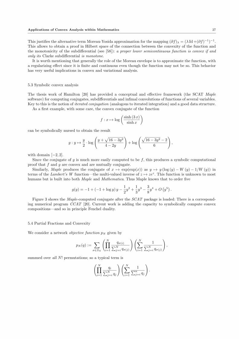
The thesis work of Hamilton [20] has provided a conceptual and effective framework (the SCAT Maplesoftware) for computing conjugates, subdifferentials and infimal convolutions of functions of several variables.Key to this is the notion of iterated conjugation (analogous to iterated integration) and a good data structure.

As a first example, with some care, the convex conjugate of the function

f : x 7→ log

(sinh (3x)

sinhx

)can be symbolically nursed to obtain the result

g : y 7→ y

2· log

(y +

√16− 3y2

4− 2y

)+ log

(√16− 3y2 − 2

6

),

with domain [−2, 2].Since the conjugate of g is much more easily computed to be f , this produces a symbolic computational

proof that f and g are convex and are mutually conjugate.Similarly, Maple produces the conjugate of x 7→ exp(exp(x)) as y 7→ y (log (y)−W (y)− 1/W (y)) in

terms of the Lambert’s W function—the multi-valued inverse of z 7→ zez. This function is unknown to mosthumans but is built into both Maple and Mathematica. Thus Maple knows that to order five

g(y) = −1 + (−1 + log y) y − 1

2y2 +

1

3y3 − 3

8y4 +O

(y5).

Figure 3 shows the Maple-computed conjugate after the SCAT package is loaded: There is a correspond-ing numerical program CCAT [20]. Current work is adding the capacity to symbolically compute convexcompositions—and so in principle Fenchel duality.

5.4 Partial Fractions and Convexity

We consider a network objective function pN given by

pN (q) :=∑σ∈SN

(N∏i=1

qσ(i)∑Nj=i qσ(j)

)(N∑i=1

1∑Nj=i qσ(j)

),

summed over all N ! permutations; so a typical term is(N∏i=1

qi∑Nj=i qj

)(N∑i=1

1∑nj=i qj

).


> >

> >

> >

> >

> >

(1)(1)

(2)(2)

(3)(3)

(4)(4)

restart:

read("scat.mpl"):read("ccat.mpl"):

with(SCAT);with(CCAT);"1. combinat,gfun,student,IntegerRelations,PolynomialTools loaded"

"2. p2s,s2p,r2p,f2p,pslq,find loaded""3. anim and binzetas loaded"

f11:=convert(exp(exp(x)),PWF);

g11:=Conj(f11,y);

sdg11:=SubDiff(g11);

Plot(sdg11,y=-1..1,view=[0..1,-5..0],axes=boxed,labels=["$y$",""]

);

Fig. 3 The conjugate and subdifferential of exp exp.

For example, with N = 3 this is

q1q2q3

(1

q1 + q2 + q3

)(1

q2 + q3

)(1

q3

)(1

q1 + q2 + q3+

1

q2 + q3+

1

q3

).

This arose as the objective function in research into coupon collection. The researcher, Ian Affleck, wishedto show pN was convex on the positive orthant.

First, we tried to simplify the expression for pN . The partial fraction decomposition gives:

p1(x1) =1

x1, (43)

p2(x1, x2) =1

x1+

1

x2− 1

x1 + x2,

p3(x1, x2, x3) =1

x1+

1

x2+

1

x3− 1

x1 + x2− 1

x2 + x3− 1

x1 + x3+

1

x1 + x2 + x3.

In [60], the simplified expression of PN is given by

p(x1, x2, · · · , xN ) :=

N∑i=1

1

xi−

∑1≤i<j≤N

1

xi + xj+

∑1≤i<j<k≤N

1

xi + xj + xk

− . . .+ (−1)N−1 1

x1 + x2 + . . .+ xN.


Partial fraction decompositions are another arena in which computer algebra systems are hugely useful. Thereader is invited to try performing the third case in (43) by hand. It is tempting to predict the “same”pattern will hold for N = 4. This is easy to confirm (by computer if not by hand) and so we are led to:

Conjecture 1 For each N ∈ N, the function

pN (x1, · · · , xN ) =

∫ 1

0

(1−

N∏i=1

(1− txi)

)dt

t(44)

is convex; indeed 1/pN is concave.

One may check symbolically that this is true for N < 5 via a large Hessian computation. But this isimpractical for larger N . That said, it is easy to numerically sample the Hessian for much larger N , and itis always positive definite. Unfortunately, while the integral is convex, the integrand is not, or we would bedone. Nonetheless, the process was already a success, as the researcher was able to rederive his objectivefunction in the form of (44).

A year after, Omar Hjab suggested re-expressing (44) as the joint expectation of Poisson distributions.3

Explicitly, this leads to:

Lemma 2 [17, §1.7] If x = (x1, · · · , xn) is a point in the positive orthant Rn++, then

∫ ∞0

(1−

n∏i=1

(1− e−txi)

)dt =

(n∏i=1

xi

)∫Rn++

e−〈x,y〉max(y1, · · · , yn) dy,

(45)

where 〈x, y〉 = x1y1 + · · ·+ xnyn is the Euclidean inner product.

It follows from the lemma—which is proven in [17] with no recourse to probability theory—that

pN (x) =

∫RN++

e−(y1+···+yN ) max

(y1

x1, · · · , yN

xN

)dy,

and hence that pN is positive, decreasing, and convex, as is the integrand. To derive the stronger result that1/pN is concave we refer to [17, §1.7]. Observe that since 2ab

a+b ≤√ab ≤ (a+b)/2, it follows from (45) that pN

is log-convex (and convex). A little more analysis of the integrand shows pN is strictly convex on its domain.The same techniques apply when xk is replaced in (43) or (44) by g(xk) for a concave positive function g.

Though much nice related work is to found in [60], there is still no truly direct proof of the convexityof pN . Surely there should be! This development neatly shows both the power of computer assisted convexanalysis and its current limitations.

Lest one think most results on the real line are easy, we challenge the reader to prove the empiricalobservation that

p 7→ √p∫ ∞

0

∣∣∣∣ sinxx∣∣∣∣p dx

is difference convex on (1,∞), i.e. it can be written as a difference of two convex functions [5].

3 See “Convex, II” SIAM Electronic Problems and Solutions at http://www.siam.org/journals/problems/downloadfiles/

99-5sii.pdf.

http://www.siam.org/journals/problems/downloadfiles/99-5sii.pdf

http://www.siam.org/journals/problems/downloadfiles/99-5sii.pdf


6 Concluding comments

All researchers and practitioners in convex analysis and optimization owe a great debt to Jean-JacquesMoreau—whether they know so or not. We are delighted to help make his seminal role more apparent to thecurrent generation of scholars. For those who read French we urge them to experience the pleasure of [44,45,46,48] and especially [49]. For others, we highly recommend [50], which follows [48] and of which ZuhairNashed wrote in his Mathematical Review MR0217617: “There is a great need for papers of this kind; thepresent paper serves as a model of clarity and motivation.”

Acknowledgements The authors are grateful to the three anonymous referees for their pertinent and constructive comments.The authors also thank Dr. Hristo S. Sendov for sending them the manuscript [60]. The authors were all partially supportedby various Australian Research Council grants.

References

1. Y. Alber and D. Butnariu, “Convergence of Bregman projection methods for solving consistent convex feasibility problemsin reflexive Banach spaces”, Journal of Optimization Theory and Applications, vol. 92, pp. 33–61, 1997.

2. M. Alimohammady and V. Dadashi, “Preserving maximal monotonicity with applications in sum and composition rules”,Optimization Letters, vol. 7, pp. 511–517, 2013.

3. E. Asplund, “Averaged norms”, Israel Journal of Mathematics vol. 5, pp. 227–233, 1967.4. H. Attouch, H. Riahi, and M. Thera, “Somme ponctuelle d’operateurs maximaux monotones” [Pointwise sum of maximal

monotone operators] Well-posedness and stability of variational problems. Serdica. Mathematical Journal, vol. 22, pp. 165–190, 1996.

5. M. Bacak and J.M. Borwein, “On difference convexity of locally Lipschitz functions”, Optimization, pp. 961–978, 2011.6. H.H. Bauschke, J.M. Borwein, X. Wang, and L. Yao, “Construction of pathological maximally monotone operators on

non-reflexive Banach spaces”, Set-Valued and Variational Analysis, vol. 20, pp. 387–415, 2012.7. H.H. Bauschke and P.L. Combettes, Convex Analysis and Monotone Operator Theory in Hilbert Spaces, Springer, 2011.8. H.H. Bauschke and X. Wang, “The kernel average for two convex functions and its applications to the extension and

representation of monotone operators”, Transactions of the American Mathematical Society, vol. 36, pp. 5947–5965, 2009.9. H.H. Bauschke, X. Wang, and L. Yao, “Monotone linear relations: maximality and Fitzpatrick functions”, Journal of

Convex Analysis, vol. 16, pp. 673–686, 2009.10. H.H. Bauschke, X. Wang, and L. Yao, “Autoconjugate representers for linear monotone operators”, Mathematical Pro-

gramming (Series B), vol. 123, pp. 5-24, 2010.11. H.H. Bauschke, X. Wang, and L. Yao, “General resolvents for monotone operators: characterization and extension”, in

Biomedical Mathematics: Promising Directions in Imaging, Therapy Planning and Inverse Problems, Medical PhysicsPublishing, pp. 57–74, 2010.

12. J.M. Borwein, “A generalization of Young’s `p inequality”, Mathematical Inequalities & Applications, vol. 1, pp. 131–136,1998.

13. J.M. Borwein, “Maximal monotonicity via convex analysis”, Journal of Convex Analysis, vol. 13, pp. 561–586, 2006.14. J.M. Borwein, “Maximality of sums of two maximal monotone operators in general Banach space”, Proceedings of the

American Mathematical Society, vol. 135, pp. 3917–3924, 2007.15. J.M. Borwein, “Fifty years of maximal monotonicity”, Optimization Letters, vol. 4, pp. 473–490, 2010.16. J.M. Borwein and D.H. Bailey, Mathematics by Experiment: Plausible Reasoning in the 21st Century, A.K. Peters Ltd,

Second expanded edition, 2008.17. J.M. Borwein, D.H. Bailey and R. Girgensohn, Experimentation in Mathematics: Computational Paths to Discovery, A.K.

Peters Ltd, 2004. ISBN: 1-56881-211-6.18. J.M. Borwein and S. Fitzpatrick, “Local boundedness of monotone operators under minimal hypotheses”, Bulletin of the

Australian Mathematical Society, vol. 39, pp. 439–441, 1989.19. J.M. Borwein, R.S Burachik, and L. Yao, “Conditions for zero duality gap in convex programming”, Journal of Nonlinear

and Convex Analysis, in press; http://arxiv.org/abs/1211.4953v2.20. J.M. Borwein and C. Hamilton, “Symbolic Convex Analysis: Algorithms and Examples,” Mathematical Programming, 116

(2009), 17–35. Maple packages SCAT and CCAT available at http://carma.newcastle.edu.au/ConvexFunctions/SCAT.

ZIP.21. J.M. Borwein and A.S. Lewis, Convex Analyis andd Nonsmooth Optimization, Second expanded edition, Springer, 2005.22. J.M. Borwein and J.D. Vanderwerff, Convex Functions, Cambridge University Press, 2010.23. J.M. Borwein and L. Yao, “Structure theory for maximally monotone operators with points of continuity”, Journal of

Optimization Theory and Applications, vol 157, pp. 1–24, 2013 (Invited paper).24. J.M. Borwein and L. Yao, “Recent progress on Monotone Operator Theory”, Infinite Products of Operators and Their

Applications, Contemporary Mathematics, in press; http://arxiv.org/abs/1210.3401v2.

http://arxiv.org/abs/1211.4953v2

http://carma.newcastle.edu.au/ConvexFunctions/SCAT.ZIP

http://carma.newcastle.edu.au/ConvexFunctions/SCAT.ZIP

http://arxiv.org/abs/1210.3401v2


25. J.M. Borwein and Q.J. Zhu, Techniques of variational analysis, CMS Books in Mathematics/Ouvrages de Mathmatiquesde la SMC, 20. Springer-Verlag, New York, 2005.

26. R.I. Bot S. Grad, and G. Wanka, Duality in Vector Optimization, Springer, 2009.27. R.I. Bot and G. Wanka, “A weaker regularity condition for subdifferential calculus and Fenchel duality in infinite dimensional

spaces”, Nonlinear Analysis, vol. 64, pp. 2787–2804, 2006.28. R.S. Burachik and A.N. Iusem, Set-Valued Mappings and Enlargements of Monotone Operators, Springer, vol. 8, 2008.29. H. Brezis, G. Crandall and P. Pazy, Perturbations of nonlinear maximal monotone sets in Banach spaces, Communications

on Pure and Applied Mathematics, vol. 23, pp. 123–144, 1970.30. J. Diestel, Geometry of Banach spaces, Springer-Verlag, 197531. M.M. Day, Normed linear spaces, Third edition, Springer-Verlag, New York-Heidelberg, 1973.32. J. Eckstein and D.P. Bertsekas, “On the Douglas–Rachford splitting method and the proximal point algorithm for maximal

monotone operators”, Mathematical Programming, vol. 55, pp. 293–318, 1992.33. S. Fitzpatrick, “Representing monotone operators by convex functions”, in Workshop/Miniconference on Functional Anal-

ysis and Optimization (Canberra 1988), Proceedings of the Centre for Mathematical Analysis, Australian National Uni-versity, vol. 20, Canberra, Australia, pp. 59–65, 1988.

34. N. Ghoussoub, Self-dual partial differential systems and their variational principles. Springer Monographs in Mathematics,Springer, 2009.

35. J.-P. Gossez, “On the range of a coercive maximal monotone operator in a nonreflexive Banach space”, Proceedings of theAmerican Mathematical Society, vol. 35, pp. 88–92, 1972.

36. J.-B. Hiriart-Urruty, M. Moussaoui, A. Seeger, and M. Volle, “Subdifferential calculus without qualification conditions,using approximate subdifferentials: a survey”, Nonlinear Analysis, vol. 24, pp. 1727–1754, 1995.

37. J.-B. Hiriart-Urruty and R. Phelps, “Subdifferential Calculus Using ε-Subdifferentials”, Journal of Functional Analysisvol. 118, pp. 154–166, 1993.

38. L. Hormander, “Sur la fonction d’appui des ensembles convexes dans un espace localement convexe”, Arkiv for Matematik,vol. 3, pp. 181–186, 1955.

39. V. Klee, “Convexity of Chebysev sets”, Mathematische Annalen, vol. 142, pp. 292–304, 1961.40. F. Kohsaka and W. Takahashi, “Existence and approximation of fixed points of firmly nonexpansivetype mappings in

Banach spaces”, SIAM Journal on Optimization, vol. 19, pp. 824–835, 2008.41. J. Lindenstrauss, “On nonseparable reflexive Banach spaces”, Bulletin of the American Mathematical Society, vol. 72,

pp. 967–970, 1966.42. P. Marechal, “A convexity theorem for multiplicative functions”, Optimization Letters, vol. 6, pp. 357–362, 2012.43. G. Minty, “Monotone (nonlinear) operators in a Hilbert space”, Duke Mathematical Journal, vol. 29, pp. 341–346, 1962.44. J.J. Moreau, “Fonctions convexes en dualite”, Faculte des Sciences de Montpellier, Seminaires de Mathematiques Universite

de Montpellier, Montpellier, 1962.45. J.J. Moreau, “Fonctions a valeurs dans [−∞,+∞]; notions algebriques”, Faculte des Sciences de Montpellier, Seminaires

de Mathematiques, Universite de Montpellier, Montpellier, 1963.46. J.J. Moreau, “Etude locale d’une fonctionnelle convexe”, Faculte des Sciences de Montpellier, Seminaires de Mathematiques

Universite de Montpellier, Montpellier, 1963.47. J.J. Moreau, “Sur la function polaire d’une fonctionelle semi-continue superieurement”, Comptes Rendus de l’Academie

des Sciences, vol. 258, pp. 1128–1130, 1964.48. J.J. Moreau, “Proximite et dualite dans un espace hilbertien”, Bulletin de la Societe Mathematique de France, vol. 93,

pp. 273–299, 1965.49. J.J. Moreau, Fonctionnelles convexes, Seminaire Jean Leray, College de France, Paris, pp. 1–108, 1966–1967. Available at

http://carma.newcastle.edu.au/ConvexFunctions/moreau66-67.pdf.50. J.J. Moreau, “Convexity and duality”, pp. 145–169 in Functional Analysis and Optimization, Academic Press, New York,

1966.51. J.-P. Penot, “The relevance of convex analysis for the study of monotonicity”, Nonlinear Analysis, vol. 58, pp. 855–871,

2004.52. J.-P. Penot and C. Zalinescu, “Some problems about the representation of monotone operators by convex functions”, The

Australian New Zealand Industrial and Applied Mathematics Journal, vol. 47, pp. 1–20, 2005.53. R.R. Phelps, Convex Functions, Monotone Operators and Differentiability, 2nd Edition, Springer-Verlag, 1993.54. R.R. Phelps and S. Simons, “Unbounded linear monotone operators on nonreflexive Banach spaces”, Journal of Nonlinear

and Convex Analysis, vol. 5, pp. 303–328, 1998.55. R.T. Rockafellar, “Extension of Fenchel’s duality theorem for convex functions”, Duke Mathematical Journal, vol. 33,

pp. 81–89, 1966.56. R.T. Rockafellar, “On the maximal monotonicity of subdifferential mappings”, Pacific Journal of Mathematics, vol. 33,

pp. 209–216, 1970.57. R.T. Rockafellar, “On the maximality of sums of nonlinear monotone operators”, Transactions of the American Mathe-

matical Society, vol. 149, pp. 75–88, 1970.58. R.T. Rockafellar and R.J-B Wets, Variational analysis. Grundlehren der Mathematischen Wissenschaften [Fundamental

Principles of Mathematical Sciences], 317. Springer-Verlag, Berlin, 1998 (3rd Printing, 2009).59. R. Rudin, Functional Analysis, Second Edition, McGraw-Hill, 1991.

http://carma.newcastle.edu.au/ConvexFunctions/moreau66-67.pdf


60. H.S. Sendov and R. Zitikis, “The shape of the Borwein-Affleck-Girgensohn function generated by completely monotone andBernstein functions”, Journal of Optimization Theory and Applications, in press.

61. S. Simons, Minimax and Monotonicity, Springer-Verlag, 1998.62. S. Simons, From Hahn-Banach to Monotonicity, Springer-Verlag, 2008.63. S. Simons and C. Zalinescu, “A new proof for Rockafellar’s characterization of maximal monotone operators”, Proceedings

of the American Mathematical Society, vol. 132, pp. 2969–2972, 2004.64. S. Simons and C. Zalinescu, “Fenchel duality, Fitzpatrick functions and maximal monotonicity”, Journal of Nonlinear and

Convex Analysis, vol. 6, pp. 1–22, 2005.65. L. Sucheston, “Banach limits”, American Mathematical Monthly, vol. 74, pp. 308–311, 1967.66. C. Zalinescu, Convex Analysis in General Vector Spaces, World Scientific Publishing, 2002.67. E. Zeidler, Nonlinear Functional Analysis and its Applications II/A: Linear Monotone Operators, Springer-Verlag, 1990.68. E. Zeidler, Nonlinear Functional Analysis and its Applications II/B: Nonlinear Monotone Operators, Springer-Verlag,

1990.

Date post:	15-May-2018
Category:	Documents
Upload:	lydung
View:	230 times
Download:	2 times

Applications of Convex Analysis within Mathematics - … · Applications of Convex Analysis within...

Documents