92
APPLICATIONS OF LINEAR PROGRAMMING TECHNIQUES TO SOr-IE PROBLEMS OF PRODUCTION PLANNING OVER TIME by R. M. Ziki and RB L o Anderson Institute of Statistios Mimeograph Series No o 2.88 1961
APPLICATIONS OF LINEAR PROGRAMMING TECHNIQUESTO SOr-IE PROBLEMS OF PRODUCTION PLANNING OVER TIME
by
R. M. Ziki and RB Lo Anderson
Institute of StatistiosMimeograph Series Noo 2.88AprU~ 1961
ivTABLE OF CONTENTS
• • 0 • • • •
• • • • • •
• • •
vi
1
Page
• •
· . .... ..
· ..
.. .• •• • •
• • • •· ..
• •.. .. .• •
.. ..INTRODUCTION 0 •
LIST OF TABLES
2.0
1.0..
2.1 Decision Problems .. • • .. .. • • • • .. • .. • .. .. • • .. •2.2 The Problem of Fluctuations in a Firm's
Production Over Time .. • • • .. .. • • .. .. .. • .. .. • ..2.3 Mathematical Formulation of a Basic Model • .. .. .. • • ..
1
26
3.0 A SIMPLIFIED MODEL .. . • • • • • • • • • • • • •• • • • • .. .. 9
3.11.23.33.43..53.63.7
A Procedure for Obtaining ¢ = Max Z .. • • .. • .. .. .. .. •Allocation to a S:i.ngle Time Period .. .Allocation to Two ~ime Periods .Two Useful Lemmas • .. • .. .. .. • .. • .. .. .. .. .. .. .. .. .. •Allocation to Three Time Periods ......... • .. • • • •Allocati on Theorems .. • .. • • • .. • .. • .. • • • .. • • ..Su.mrnary • • • • • • • • • • • • • • • • • • • • • • • •
9111112131827
The Simplex Computational Procedure • .. .. • .. • • .. .. •The ll1al Problem of Linear Programming ..
The Problem of Line ar Programming .. .. .. • • • • ..Brief Mathematical Background .. .. • • .. .. • .. • •Properties of a Solution to the Linear Programming
Problem • • • • • • .. • • .. • • • • • • ......
4.0 LINEAR PROGRAMMING •
4.14.24.3
4.44.5
.. . . .. . . • • • • .. .. .. . .. .. • • · . .... . ... .. ..
.. . .
29
2930
323540
5.0 USE OF THE LINEAR PROGRAMMING PROCEDURES FOR THE PRODUCTIONSTABILIZATION PROBLEM .... .. .. • • • .. • • • • .. • .. ... .. ..
A Linear Programming Formulation of the ProductionStabilization Problem. .. .. • .. .. • ... .. .. .. .. .. .. ..
A Line ar Programming Formulati on of the SimplifiedModel • • • ., • • • • • • • • •• • ... ••• • • • •
A Solution for the Simplified Problem by the SimplexMethod. • .. .. .. .. .. • .. • • • • • .. .. • • .. • • • ....
A Useful Initial Basis to Start the IterativeProcedure for Solving the General ProductionStabilization Problem .. .. .. .. .. .. .. .. • • .. • 0 0 0 ..
A Criterion for Selecting the Vector to be Introducedinto the Basis .. .. .. • • .. .. .. .. .. ..
.. Procedure for Finding the Optimal Solutions (One orMore) to the General Production StabilizationProblem for Each Value of c in the Interval c ~O ...
41
43
45
60
68
74
TABlE OF CONTENTS (continued) v
.Page
6.0 SUMMARY AND LIMITATIONS AND ElTENSIONS OF THE STUDIED MODEL 77
o e 0' e • • • • • •
601 Sunnnary 0 0- 0 • • • e 0 6 0 e 0 e e & • • 0 • • •
6~2 Limitations and Extensions of the Studied Model •
LIST OF REFERENCES 0 & 0 • & • • • 0 0 0
• •• •
7783
87
3,,1.
.. 5.1•
5.2.
5.3,.
5.. 4.
5.5.
vi
1.0. LIST OF TAB LBS
Page
Optimal allocation plans for the simplified model, (3.01). 28
Simplex tableau for B(l) e .. .. • .. 48
Simplex tableau for B(.f,) .. ".. .. .. • • • • • .. • • .. • .. • •• 52.
Simplex tableau for B(T). • .. • • • • • .. .. • • .. • • .. • ... ~7
Simplex tableau for B(T+l) e .. " " ".. 61
Matrix formulation of linear constraints for the generalstabilization problem <) <) .. .. • ••• 62
2 0 0 INTRODUCTION
2 0 1 Decision Problems
A decision problem arises when it is necessary to choose from arnong
various alternate courses of action9 one of which is best according to a
certain criteriono Although the art of making optimal decisions is as
old as mankind9 the mathematical theory of decision-making is a new
development 0 Careful mathematical formulation of many economic~ mili-
tary and other problems helped in the development of mathematical tools
needed for their solutiono On the other hand, development of statistical
decision theorY9 linear and non=linear prograrnming~ game theory and
queuing theory resulted in new practical disciplines, such as operations
researchjl management science9 and systems analysis o All of these are
basically concerned with the sarne task~ to analyze various feasible courses
of action with a view to determining which course offers the fullest
desired satisfactiono A decision problem typically has four parts
[Karlin9 1959] ~
98(1) A model expressing a set of assumed empirical relationsarnong the set of variables o
(2) A specified subset of decision variables~ whose valuesare to be .chosen by the firm or the decision-makingentity 0
(3) An objective function of the variables, formulated insuch a way that the higher its value~ the better the6ituation is from the viewpoint of the firmo
(4) Procedures for analyzing the effect on the objectivefunction of alternative values of the decisionvariables o
llt
2 0 2 The Problem of Fluctuations ina Firm t s Production Over Time
It has long been realized that fluctuations in a firm's produc-
tion over time may have some disadvantages.. SUch fluctuations cannot
always be avoided; this is the case for many agricultural products,
since seasonal variations in weather conditions may make it impossible
to produce some crops except in a particular season. If weather con-
ditions permit.j) the farmer may avoid having idle land and equipment
by rotating suitable crops in successive seasons within a year"
The problem of fluctuations in production is not, however,
limited to agricultureo A manufacturing firm, for example, may be
faced with a fluctuating monthly demand for its product. If' the
demand is known or can be accurately predicted, the firm faces the
problem of choosing from among many production schedules which
satisfy the monthly requirements.. For example, the firm can produce
each month approximately the amount required in that montho However,
this fluctuating production schedule is costly to maintain because of
overtime costs in high=production months and because of costs asso-
ciated with releasing personnel and machinery in low production
months" On the other hand, the firm can overproduce in months of low
requirements, store the surplus, and use the excess in months of high
requirements" The production can thus be made quite stable" However,
because of storage costs~ such a schedule may not be the most efficient.
This illustrates the diffieulties that can arise if there are conflic-
ting objectives inherent in a problem" What is required, in problems
,,,",
-3-
of this kind is a production schedule that minimizes the sum of the costs
arising from fluctuations in production and from storage.. In other words»
the optimal schedule is one which compromises between the conflicting
objectives 0 For a particular problem, the optimal schedule will depend
on the relative magnitude of the two types of costs o A modification of
this problem is obtained by assuming that there are no market limitations
on the quantity that the firm can sell at any given month but that prices
follow a seasonal patterno Given certain limitations on the producing'
and storing capacities of the firm,l) it is required to find how much the
firm should produce, store,l) or sell during each of a specified number of
months 0 In the programming literature» problems of this type are termed
"production=scheduling and inventory control problems.," Riley and
Gass [1958] give a comprehensive bibliography of published papers
written on the different aspects of these problems o Obviously a basic
characteristic of the commodities involved is that they must be non
perishable.,
For perishable commodities,I) stabilization of production over time
may not be aClhieved by storage o However» if it is technically possible
to produce the commodity at any time within the yearf) it may be advan
tageous to the firm producing such a commodity to explore the possibility
of planning its production over time in such a way as to reduce fluctua=
tions in production., An example of au ch a commodity is the banana/) We
will summarize here some economic characteristics of the banana discussed
by SJ.mm.onds [1959J ~
(1) The banana is a highly perishable fruit which can be
harvested for a distant market during a very limited
period of the life of the buncho
(2) Bananas can be produced at any time of the year o The
producer'can to some extent affect the time at which
the banana tree matures o This could be done by
either varying the time of planting, by pruning (con-
. trolling of fo11owers)~ by changing the rate of ferti
lization used, or by a combination of these o
(3) Factors that can affect the yield per tree are:
location, rate of fertilization, and the time at which
the tree matures o
(4) The price of the banana depends on the availability of
other fresh fruits and in general follows a seasonal
pattern 0
(,) The peculiar demands made by a banana cargo are such
that ships mst be especially designed and constructed
for the job; they~e not, in general, suitable for
carrying other cargoes o
(6) One effect of the perishability of the fruit is that
the producer is at the economic mercy of the shipping
organization0 As a result, some producing companies
found it necessary to own the ships needed for trans
porting their bananas to world markets o
-4-
....
From these characteristics it can be seen that (a. firm engaged in
producing bananas has an interesting decision problem" The firm has to
decide on a production schedule that maximizes its profits in the face
of certain restrictions. In gener,al, the 'restrictions faced by any firm
maybe classified into two groups: those set by technological restric-
tions (e"g", available methods of production and shipping requirements)
and those set by conditions in the market (e"g", prices and market
capacities).. W.e will follow a suggestion made by Charnes, Cooper and
Farr [195$.) :UtA useful beginning to many facets of optimal programmingmay be made by determining what might be called thecompany8s 'plant profit potential. I By assuming purelycompetitive conditions so that current prices constitutethe only market limitation, a measure of maximum profitpotential can be securedo "
It must be recognized, as the authors point out, that the magnitude of
profits and the character of the optimal solution vary with changes in
the structure of prices" Moreover practical sales considerations may
make it impossible to s ell what is technologically, at given ,prices,
the best to produce.
The optimal solution obtained under the a bove assumptions, is,
nevertheless, of interest.. It provides a basis of long range sales
and prcduction planning. It also provides a basic structure of
computations which can be used as a baginning for other calculations ..
For example, restrictions on the amounts that can be sold in any given
time period may be added to modify the solution obtained without these
restrictions ..
In the next section a mathematical model is formulated to study the
decision problem f aced by a tirmthat has to spend large amounts of
capital on a specialized factor that could be idled part of the time by
fluctuations in productionc
2,,3 Mathematical Formulation of a Basic Model
Assume that a firm has under its control f different resources;
e"g"9 areas of land available to the firm at different time periods for
starting a new production process9 or areas of land in different locations"
Let Nr be the amount of the r th resource (r ... 19"",,~f) that is available
to the firm" The time interval in which it is technically feasible for
the firm to produce1 using any of the the f resources, is divided into T
equal time periods 0 We make use of the following ~
~t ... the p art allocated by the firm from resource r to
produce in the t th time period (t := l~ 0 0 0 ~T) 9
Yrt ... the yield or output per unit of nrt; ioeo,9 the yield
obtained in the t th time period from a unit of the
thr resource o
the price per unit of the commodity in the tth time
period minus the direct variable costs needed to obtain
one unit of the commodity in the tth time period from
the r th resource" 1/
1/ D'irect variable costs in 'Prt are to include any variable costs
realized in either the production process or in transportingthe commodity to markets (e"g,,~ fertilizer costs and fuel costs)"
a ~ the cost per unit of a certain factor 5 (e"go, a ship)
for being available in any of the T tim.e periods o We
will assume that the units of the factor S, are of the
same type and thus are completely interchangeable in
their useso
b ~ the quantity of the commodity that can be accommodated
by a unit of factor a in a tim.e periodo
The number of units of the factor S needed during the T time periods
is the maxinro.rn output by the firm in any of the T time periods divided by
b; if this ratio is not an integer, use the next largest integer" If b
is relatively large compared With the maximum output that can be pro-
duced by the firm in any of the T time periods, the number of units of g:
needed by the firm is approximately the same for any production plan.. In
this case
C ""' a 0 [the number of needed units of SJcould be taken as a fixed costo However, if b is relatively small
compared with the maximum feasible output, we cannot consider C fixed,
since this maxinro.rn is a function of the allocation plan chosen by the firmo
The number of needed units of S, can be approximated tlby
~ [the max:i.mum output by the firm in any of the T time period~
~ ~ Max [ ] nrtyrt] 0
t T""l
tI The approximation is a result of the above~mentioned iildivis~ .-,ibilityo
-8-
This approximation obviously imp~oves with the increase in the relative
magnitude of the maximum output to b. Hence,
o
e:= a Max'6' t
where c =alb.
Under the above aSSlllllptions, the decision problem faced by the firm
may be summarized as follows:
Find the allocation plan:
Which maximizes the objective function
Sllbjectto the restrictions
T
]nrt~ Nr and nrt~O; r = l, ...,f; t =1, ...,T.tal
3.0 A SIMPLIFIED MeDEL
In this section the analysis of a simple model will be used to
illustrate some basic characteristics of the problem.
If there is a single resource that could be channeled to yield an
output in time periods, t = 1,2" ...,t, ... "T, the subscript r(in Section
2.3) could be dropped from Nr,nrt'Yrt and Prt.
Assuming that PI = P2 =: ••• =: Pt = PT =: P> 0, the problem
is to maximize
T
Z; = P~ ntYt - c Max rIl:1Yl' ...,ntYt' •""~YT1 "t=l L'
subject to the conditions
T
]~~Nt=l
and
(3.01)
(3.02 )
(3.03)
t =1, •••"T. (3.04)
Definition: A feasible solution to the problem is a solution
~I = (nl,n2' •••"~' •••'~) which satisfies conditions
(3.03) and (3.04).
It is clear that there are infinitely many feasible solutions to the
problem. Among these, it is required to find a solution which maximizes
3.1 A Procedure for Obtaining ¢ = Max Z,
'Without any loss of generality, let the yields be arranged. "as follows:
(3.11)
-10-
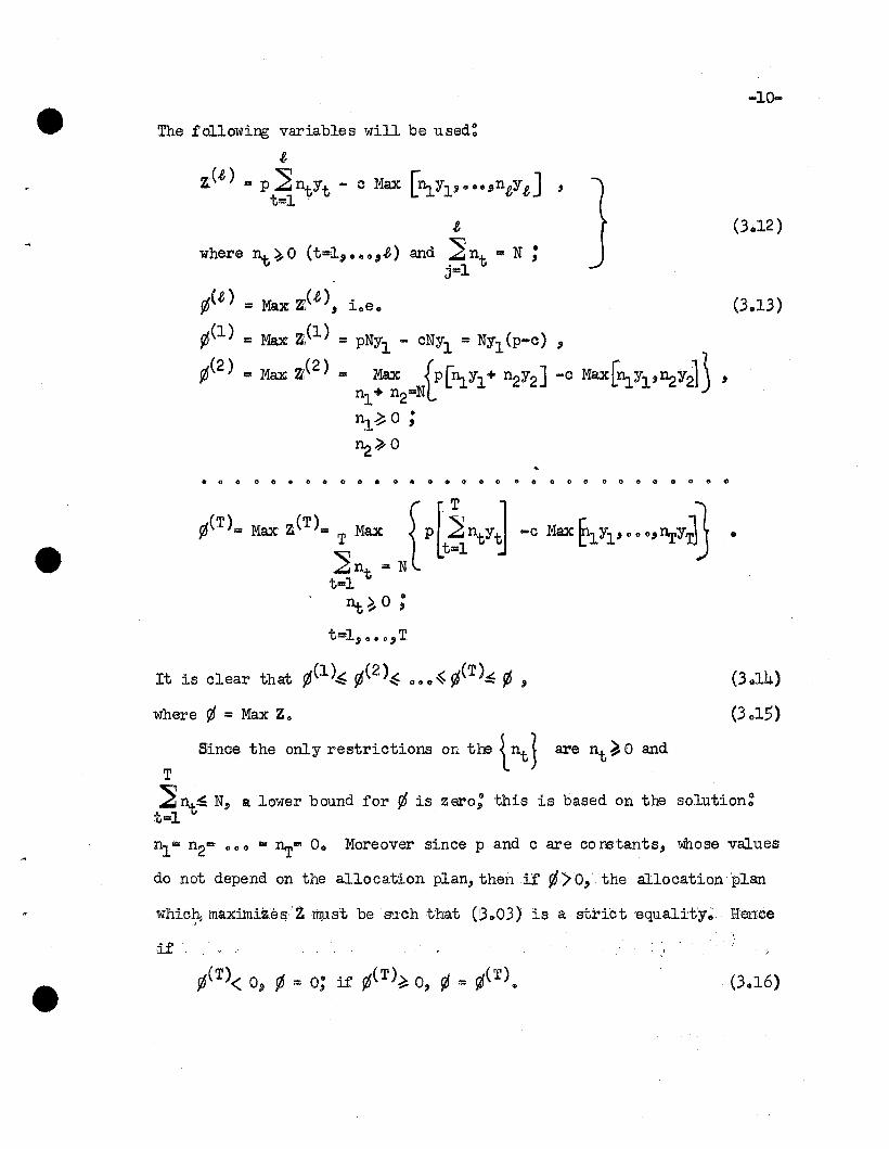
The following variables will be used:
tz.(t) =p~ntYt - c Max [tl:1.Yp .. u,n,eYtJ '
tel
,e (3.12)where nt ~ 0 (t=l.ll" u"t) and ~ nt = N ;
j=l
¢(t) = Max z:(t), i"e. (3.13)
¢(1) = Max ~(l) = pNYl .. cNY1 = NYl (p-c) ,
¢(2) ... Max ~(2) = Max [P[~Yl+ n2Y2] -c Max[~Yl'~Y21J 'nl+ ~=NL
nl~ 0 ;
~~O
.0000.0.00 ••••• 0-000.0000-0000000
t=l, 0"'" T
It is clear that ¢(l)",¢(2)~ "o,,~¢(T)~¢,
where ¢ = Max Zo
Since the only restrictions on the tntJ are nt ~ 0 and
T
~nt~ N, a lower bound for ¢ is zero; this is based on thetel
(3.14)
(3015)
solution:
~ 0= n2= 0"" '" ~= 0.. Moreover since p and c are co nstants, whose values
do not depend on the allocation plan, theni! ¢>O,the allocation plan
whic~, maximiz,8I:j'Zmp.s"t be SUch that (13 ..03) is astrict 'equality; Hence
(3016)
(3.21)
-11
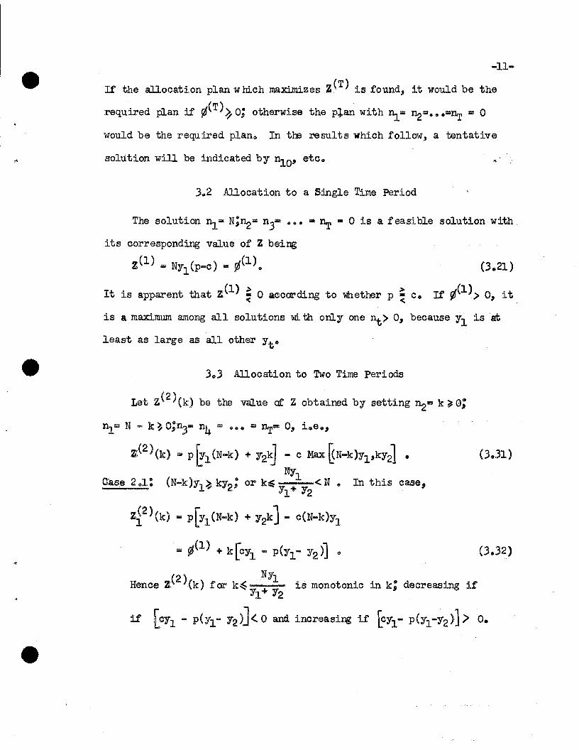
If the allocation plan wmch maximizes Z(T) is found, it would be the
required plan if !I(T)~ 0; otherwise the p~an with Il:L"" ~=.H=~ • 0
would be the required plano In tJ::e results which follow, a tentative
solution will be indicated by n10, etc.
3..2 Allocation to a S:ing1e Time Period
The solution n1'"' N;~= n3= .... '"' n.r = 0 is a feasible solution with
its corresponding value of Z being
Z(l) ~ NYl(P-c) '"' !I(l) ..
It is apparent that Z,(l) ~ 0 according to whether p Sc. If !tel»~ 0, it
is a maximum among all solutions 'Wi. th only one ~> 0, because Yl is at
least as large as all other Yt"
303 Allocation to Two Time periods
Let z(2)(k) be the value at Z obtained by setting n2= k ~O;
...
nr= N = k ~ 0;n3"" n4 '"' ..... == ~- 0, i.e.,
z;(2)(k) § P~I(N-k) + Y28 - c Max~N-k)Yl'kY21 •
NYlcrase 2 01: (N-k)Yl~ kY2; or k~ < N.. In this case"Y1+ Y2
Z~2) (k) "" P[Y1(N-k) + Y2k) - C(N-k)Yl
"" flI(l) + k[cYl ... P(Yl- Y2)] .. (3.32)
(2) NYIHence Z: (k) for k~ is monotonic in k; decreasing if
Yl+ Y2
if [ 011'" pC Yl- Y2)J <. 0 and increasing if [cYl- P(Yl-Y2)] > O.
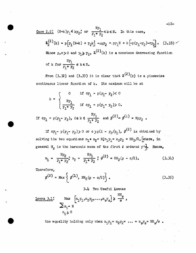
-12-NYl
c.a.se 2 0 2: (N-k)Yl~ kY2; or Yl
+ Y2 ~k~N. In this case,
~2)(k) "" P[Y1(N-k) + Y2kJ - ckY2 =.Py1N + k~P(YI-Y2)-CY~. (3.33)'/
Since p,c>°and Yl~ Y2' z,(2) (k) is a monotone decreasing function
NYlof k for ~ k ~ N.
Yl+ Y2
From (3.32) and (3.33) it is clear that Z(2)(k) is a piecewise
continuous linear functi on of k. Its maximum will be at
(3.34)
NYl (2) (1)If oY.l "" P(Yl- Y2):; O~ k ~ and ¢ c, ¢ = Npy •
Yl+ 1a 2
If 0Yl- P(Yl- Ya»O or c)p(l- Ya/Yl)' ¢(a) is obtained by
solving the two equations nl + ~= N;~Y1= naYa = NHa/a, ~here$ in
general H.e is the harmonic mean of the first .e ordered y.~. Hence,
NY2 NYl (2)n.. "" : na =< ; rj ::0 NHa(p - c/2).
.L Yl+ Y2 . Yl+ Y2
Therefore!)
¢(2) - llaxt¢(l), ~(p - 0/2») • (3.3.5)
.. -
-13-
Proof: The solution to this set of s independent equations:
s
~lni :=0 N, ~Yl= n2Y2= 0 .. = nsys is niYi = NHs/s.J.=
Any depa.rture from equality of the lniYiJ must make at least one
of the { ni YiJgreater than NHs/s.
r, 1 NHsLemma 3.2: Min lnlYl'~Y2)O"JnsYsJ ~ S- J
]ni = N
ni~ 0
the equality holding when ~Yl= ~Y2= ... =' nsys· NHs/So
Proof': As above, any departure from equality or the i~1i}also mst make at least one of the 1niYi) less than NRs/s.
3.5 Allocation to Three Time Periods
Let zO) (k) be the value of ZOtbtained by setting n3= k ~O.. Then
¢O) (k) =- Max. [zr~) (k)] ; ¢O)= Max r¢cn(kil,nl + ~:=o N-k O~ k~Nr
~,~~O
where z(3)(k) ... P(~Yl+ ~Y2+ ky3) - c Max &YlI~12,kY~ • Hence"
¢(» (k) • pI,,),,· Max [p(":!.YJ.+ "2Y2) - • Max [":!.Yl.'''2Y2'ky3]1 •. ~+~ ... N-kl J
~,n2~ 0
12Case 3.1: 011- P(Yl- 12) ~ 0 or c/p~l - 1. .. In this case, the interval
1
(o~ k~ N) is divided into the follow:ing three sub-intervals:
In II' Max rI1.Yl'~Y2,kY3]'" '. Max . [I1.Yl'~Y2J ' since11..+ ~= N-k'- n1+ ~= N-k
NHby Lemma 3.1 -l- ~ Max: [~Yl'~Y2,kY31 ' the equality holding only when
I1.Yl= n2Y2= kY3= NH3/3. Hence, from the results in section 3.3,
~Yl= ~Y2= (N-k)H2/2 and
¢f~)(k) = pkY3 + (N-k)H2(p - c:,/2) = ¢(2)+ k [C~2 .: p(H2'- Y3)] •
(3.51)
In ~, it appears that ¢~3)(k) is obtained bysalving the follow:ing
equations:
niY2- [N-k(1 + 1/'"1>] '"2 &; (N -~ (Yi + Yi">] '"2
r. H3 3 1] NH3=NY2 Ll - "3 (ifj -12) ... T 0
NH3 NH3 r: ]Since nlYl'" kY3 ~ T am n2Y2 ~ T ' Max (1.Yl'~Y2,kY3
z~3)(k) =< kY3(2p-c) + PY2 [N - k(l+ Y3/Y1)J
== NPY2 - k [Y3(CY1- PYl+ PY2)/Y1'" P(Y2- Y3)J •
..
SUppose we change .(3.52) as follows:
I1:l0 = 11. + 5 and ~O = ~ - 5, 0< 5~N - k(l + Y3/Yl)'
In this case, Max [I1:l0Yl'~OY2,kY~ == (11.+ 5)Yl and ~~3)(k) would be
changed by 5 [P(Yl- Y2) - eYlJ ~ O. Similarly if
I1:lo == nl - 5 and ~O = ~ + 5, 0<' 5~ kY3/Yl ,
Max [~OYl'~OY2' kY3] == Max [n20Y2,kY31 ==
== Max L(N-k - ky3Yl + 5)Y2,ky3J •
Hence z~3) (k) would be changed by -5p(Yl- Y2) - cA, A~ 0"
where
[
0.' if ky3~(N-k-ky3/Yl+ 5)Y2';A= .
(N - k - kY3/Yl + 5) Y2- ky3 at 'k:'Z3«N-k~:,IYi~·8)Y2 :~.
In either case, ~3)(k) would be decreased; hence ¢~3"(k) is given
by (3 ..53)e Since cYl- PYI+ PY21t 0 and Y2~ Y3' ¢~3)(k) is a monotonically
non-increasing function of ko Hence ¢~3) (k) is a maximum. when
kY3= NH3/3; i.e.,
(3) NH3 [NH3 ]¢a .. T (2p-c) + PY2 N - 3Y3 (1 + Y3/Yl)
NH3 r H3 1 1 J== T (2p-c) + NPY2 L1 - )' (Yj + Yi)
"" NH3(p - c/3} :0 ¢13>[k == NH/3J •This checks that the maximum value of ¢~3) is the same as the value of
¢i3) at its maximum value of k; hence, ¢(3) is not in the second
interval.
(.3.56)
-16-
In I.3' it appears that ¢iJ,) (k) is obtained by setting ~.. N - k,
~ - O. In this case kY.3~ (N-k)Y1; hence,
Max: [~yp~Y2,kY.3J ~ ky.3.
Therefore,
1l1.3)(k) :=0 P [(N-k)Y1+ ky.31-CkY.3- NPY1- k [P(Y1- Y.3) + CyJ ,(.3.55)
which is a monotone decreasing function of k.
Suppose ~O ... 5 and ~O = N - k - 5, 0< 5~N-k;Max [~OYl'~oY2,ky.31
i~ still ky.3 and z,~.3) (k) is changed by 5P(Y2- 11) ~ O. Therefore,
¢~3)(k) is given by (.3.55) and
0) NY1 r: J NY1Y.3¢) - NPY1- Y1+ Y.3 t.:(Y1- Y.3) '* cY3 ... 11+ Y.3 (ap - c)
(.3) C· . Ny± 1III ¢2 .k ... Y1+ YiJ •
.. be concerned with the first interval; i.e.,
-17..
Case .3.2: cYl- p (Yl- Y2) <O. For this case, we have s IDwn previously
that ¢(2) =¢(l) = NYl(P-c)o We also assume that ¢(3)(k) is
obtained by setting ~ = N - k am ~ = oi in vh ich case
Max [nlYp~Y2,kY31:1 Max U-N-k)YPky3] <)
z,(J) (k) • ) Nh (P-.O) + k [- P(Y1- Y3) + OY1] , if k ="iLNYIP + k fr(Yl- Y3) - cy3J:I if k = k2"
Suppose we consider ~O "'" 8 and I1.0 I: N - k .. 8, 0 < 8 ~ N-ko
For k I: k1' Max [<N-kl,,",8)Y1'8Y2,klY31 can be anyone of the three,\)
depending on the magnitude of 80 Hence the change in z,(3)(~)
will be ~ 8 [( ... P(Yl- Y2) + CYll < 0 0 For k =' ~.Il
Max ~N-k2-8 )Y1' 8Y2,9k2Y3] =- Mo: [8Y2.1lk2Y3J 0 In this case the
change is ~ .... 8p(Yl- Y2)<"00 Hence ¢(3)(k) for Case 30 2 is given
by (3059).. Again we note that ¢(3)(kl ) is a monotonic decreasing
function of ~,9 since .. P(Yl.... Y3) ... cYl~ - P(Yl- Y2) + cYl<0;
similarly for ¢(3)(k2)o Therefore for Case 3 0 2, /:~'\
91(3)= NY1(P ... c) I: ¢(l)o
-18-
3.6 JUlocation Theorems
The allocation plan for two time periods is one of the following
cases:
(a) nl "" N, n2 "" 0;
(b) nlYl "" n2Y2' nl + ~ "" N.
W:e note that both solutions have the following property:
Similarly, the allocation plan for three time periods is one of the
follow:ing:
(a) ~ "" N, ~ "" 0, n3 "" 0;
(b) ~Yl = n2Y2' ~ + ~ = N, n3 = 0;
(c) ~Yl = ~Y2 "" n3Y3' I1. ... ~ + n3 =:0 No
Again for (a), (b), or (c), ~Yl~ ~Y2~ n3Y30
This suggests the following theorem.
Theorem 3.1:
..
two positive constants, the allocation plan Which maximizes
T() ~... [ Jz. T == P ~~Yt ... c Max~lYl'oo •.9~YT ,
t=l
subject to the restrictionsT
nt~O.9 t "" 1,,,oollTll and ~nt = N"tal
has the following property: ~Yl~ n2Y2~ ••• ~¥T"
Proof: Let Z~T) be the value of Z{T) when
nt oY£ "'" ~+l oYt+' and ~ 0 + nt +Lo =< no' for Yt> Yt+l .9, ,:J. , '"where O~no< N. Therefore,
()[
2n 1. Y ~. [n y: Y ]z: ~ ... p ··0 t t+l + ~ _ c Max 0 t t+l , U ,o Yt+ Yt+l Yt"" Yt+l
In general, let llt"'" nt,o + 6~0 and llt+l= nt+l,o- 01-0, so that
nt + nt +l = no; hence»
(T) [2nbYtYt+l ~z: .... p Y +0 Y + et + 6(Yt- Yt+l)t t+l
Since Max [lltYVllt+olYt+l] ~ nt»oYt
that can occur are:
by Lemma 3.1, the only cases
...
(a) U ~Max: [lltYt"llt+1Yt+~ llt"oYt ;
~(T) = ~(T) ... p6(v ... v )o ~t ~t+l 0
(b) MaJe" [lltYt.!Jnt+1Yt+l]>u~nt"oYt ;
Z(Tt Z~T)... p6(Yt"" Yt+l) - cLMax ~tYt.tllt+1Yt+~ ... UJ"(c) Max: [ntYtj)nt+1Yt+lJ~nt.!JOYt> U ;
Z(T)_ zeiT). P5(Y~- Yt+l) - • {Max EtYt'''t+1Yt+~ - "t,oYt) •
In all cases, if 8 <0, Z;(Tt Z(T)< 0; ·therefore, 6 ~ 0; i~eo,o
nt Ytf nt+1Yt+P for all to In other words, a necessary condition
for a solution to be the maximum solution is that
Theorem 3.2:
.&-1 .&
If (.&-1). - Yo ~ L <clp <.& _ Y ~ 111 t=l Yt .&+1 t=l Yt
, for
-20-
T
"a: = p~ntYt - c Max rnlYl' ... ,ntYt'''.'~Y'l'J 't=l L I
T
subject to the conditions ~nt~N ~nd nt~ 0, t=l, ...,T,t=l
is given by .&
{
N/~ Lt=l Yt
n y. = 't to
,
,
t=l, ••• ,.&,
t = t.t1, •• • ,T •
Proof: We will first prove that the optimum allocation using
"... '&-1
:e period~ wh~~ c/p) ('&-1) - Yo ~ (Ly ) is given by (3.61).. 1It~ t
.&-1
Then we will further prove that, if c/p. <(.&-1) - Y.& ~ (1..),, t=l Yt
the optimum allocation has n.& = O. These results have already
been proven for .& = 2 and 3. The method of proof is to assume the
above is true for .& periods and prove it holds for ('&+1) periods.
In other words, it is assumed that if
.&-1
c/p >.&-1 - Y.& ~ (1..)t=l Yt
.&~··l
= N(.&p-c)1~~--).t=l Yt
(3.62 )
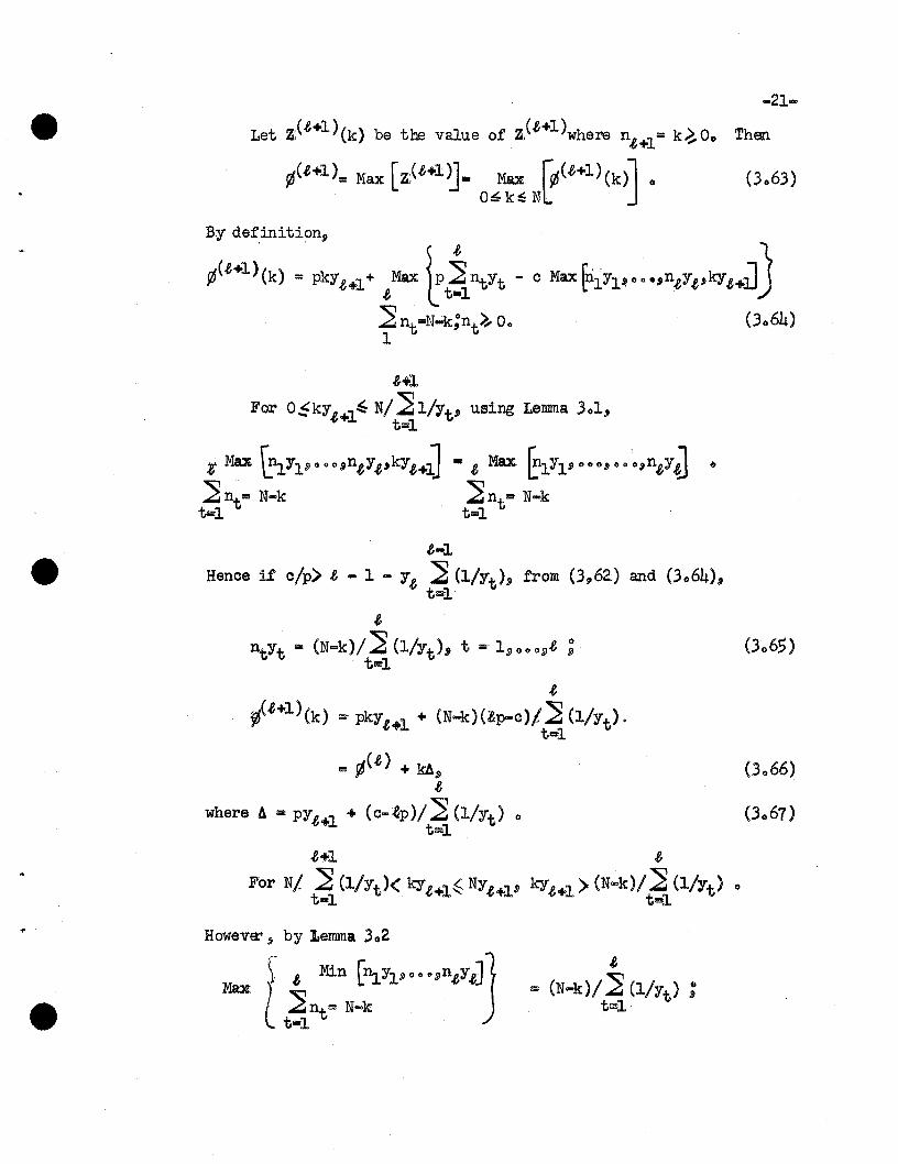
-21
Let Z;(t+l)(k) be the va.lue of Z,(t+l)where nt
+1= k~Oo Then
¢(t+l). Max [z:(t+l~lII!l Max r¢(t+l) (k)] 0 (.3063)O~k~ NL
t+l
For O~kYt+l~N/~ l/Yt, using Lemma 301,t=l
:p; Max GIY19 0 00 "ntYt,kYt+J
~nt· N-kt=l
t-l
Hence if c/p> t ... 1 ... Yt ~ (l/Yt), from (.3,62:) and (.3064),t=tl
t
D..tYt - (N=k)/~ (l/Yt)' t ... I" ()O o,9t ; (.3()6,)tal
t
ilt +1 )(k) =< pkYt+l + (N-k)(:&p-e)/~ (l/Yt).tal
lII!l ¢(t) + ~9 (3066)t
where A :: PYt+l + (c-:tp)/~ (l/Yt) 0 (3 0 67)t=l
t~ t
For Nl·~ (l/Yt)< kyt+l~NYt+p kyt+l> (N"'k)/~ (l/Yt) 0
t~ t~
...
t>= (N-k)/~ (l/Yt) ;. t!ilill
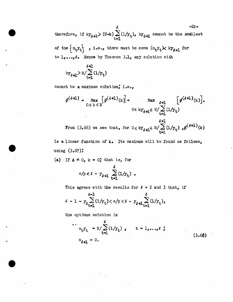
, ~-
therefore, if kY'+l> (N-k) ~ (l/Yt), ky'+l cannot be the .smallesttal
of the tIl.tYt3 ' i.e." there must be some (ntYt)< kY'+l for
t= 1, ...,'. Hence by Theorem 3.1, any solution with
.e+l
kY.e+1> Nl~ (l/Yt)tal
cannot be a maximum solution; i.e.,
91(.e+1) = Max [¢<'+l)(k~ = Max [91(.e+1)(k)].o~k~N .e~
o~ kY.e+l.f N/~ (l/Yt)tal
'+1From O.66} we see that, for o~ ky.e+l~ N/~ (l/Yt) ,¢('+l}(k)
tal
is a linear function of k. Its rnax:i.mum will be found as follows,
using (3.67):
(a) If A " 0, k == 0; that is, far
.ea/p <, - Y.e+1 ~ (l/Yt) •
t=l
This agrees with the results for' = 2 and 3 that, if
'-1 ,.e -1- y,~(l/Yt)<C/P<.e- Y.e+l~(l/Yt}'
tal tal
the optimum solution is,... 'ntYt == N/~ (l/Yt) ,
t=lt = l, ••• ,.e ;
(3068) ,
$+1
(b) For A> 0, kY$+l == Nt] (l!Yt); that is, fort=l
.eo/p) $ - Y$+l] (l!Yt). Henoe from (3.65),
t!l!ll
$+1
ntYt = kY$+l = N!] (l!Yt)~ t =1, 00 o~.e.t!l!ll
$ .e-l
Since Y.e+1~Y.e,ll .e ... Y.e+1 ] (l/Yt)~ .e-l-y.e ] (l!Yt) ;tal t=l
-23...
henoe, this solution also holds for the postulated interval.
.e-l
o/p).t ... 1 - Y.t ] (l/Yt) 0
t-1
(0) For A := 0, any value or k in the interval
.e+l
O~ kY.e+l" N!] (l/Yt) is optimal; the remainingt=l .
nt (t .. 1» 0 oO.jl.e) are given by
.entYt = (N...k)!] (l!Yt) 0
t=l
Henoe we have shown t ha.t ¢(.e) is given by (3062).9 us ing the
solution (3061), if .e-l
c/p /'" (.t-l) ... Y.t] (l!Yt) ;t=l
also that "r(.e+1) 88 d(.e) (n • 0) if)£'. P .t+l
.t
c!p<./, ... Y./,+l ] (l!Yt) 0
tal
-24-
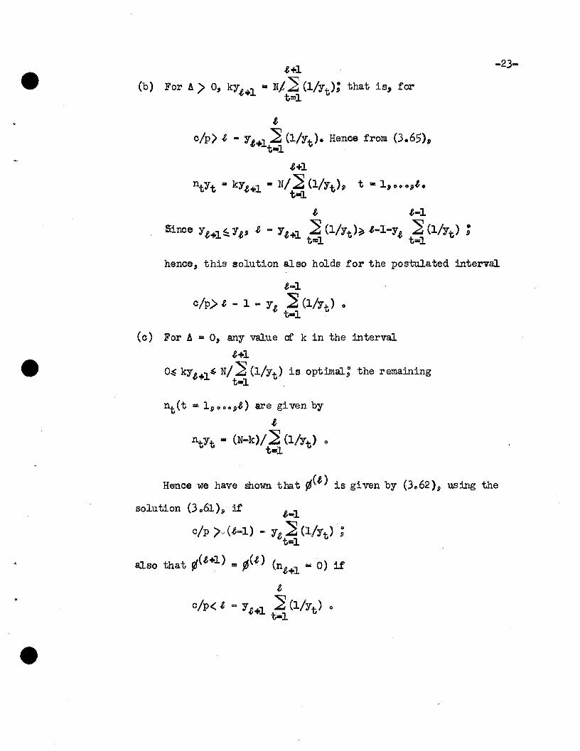
There remains to prove that in the interval
8~ 8
(8-1) - Y8 ~ (l/Yt)< c/p <8 - Y8+1 ~ (l/Yt)t~ t~
, t =8+1, 000' T 0
In other words" we wish to prove that all ~.. t >8.. are zero.
tetus·consider
¢(8+2 ) (k) = MsJc. z:(8+2) (k)8+1
n8+2= k; ~~ lit N ... kt=l
(3 0 611)
8+2:
For kY8+2> N/ ~ (l/Yt)~ no maxinnun solution could be obtained"t=l
8+2
using the same argument as above 0 If' O~ky8+2~ N/~ (l/yt)" thetal
Max: t 1of (30611) is simply 91($+1) with N replaced by (N-k)o But
for interval (3069), the opt:i.nnun solution is (3068) with N
replaced by N - k o If k> 8,n8+1Y8+1 .. O( kY8+2 =n8+2Y8+2:: ;
however this cannot be an opt:i.nnun solution by Theorem 2 01. There
fore k must equal 0;i.e09 91(8+2) is obtained from the solution
ft
tN/~ l/Ytt8Ol1
o t • t+1,t+2: 0
rIi
'" .
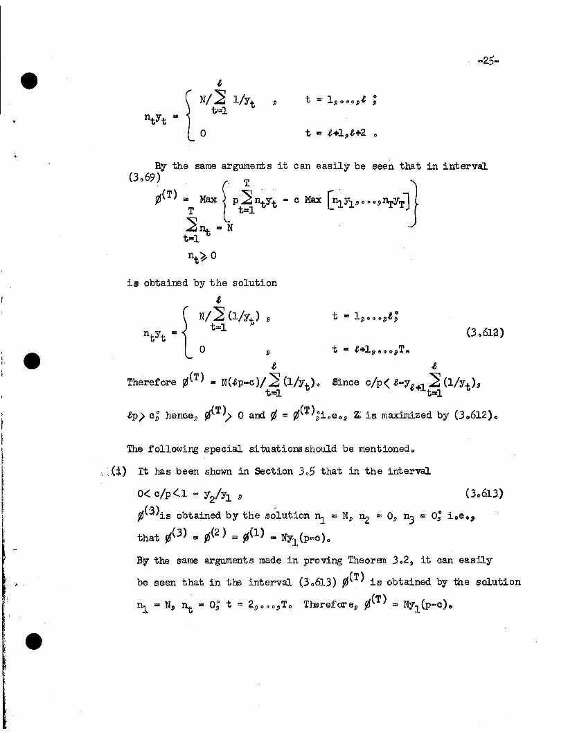
BW the same arguments it can easily be seen that in interVal
(3069), . 'n ~¢(T). I!aJ< \. p]11t7t - c !lax [":1.71" ."¥T1
T Lt=l ~J
~Ilt = Nt-l
nt~O
is obtained by the solution
ft
tN/t~ (l/Y:t) 9
ntYt =o ~
ft ft
Therefore ¢(T) "" N(tp-c)/~ (1/Yt) 0 Since c/p( t"Yft+1~ (l/Yt),t~ t~
ftp) c; hence, ¢(T») 0 and ¢ = ¢(T);Leo, Z; is maximized by (0612)0
The folloWing special situations should be mentioned o
It has been shown in Section 305 that in the interval
0< c/p <'1 "" Y2/Y1 9 (30613)
¢(;))is obtained by the so'lution ~ 118 N, ~ "" 0, n3 "" 0; ioeo"
that ¢(3) Ill! ¢(2) 18 !del) ... NY1 (p"'C) 0
Ry the same arguments made in proving Theorem 3 02, it can easily
be seen that in tre interval (30613) !I(T) is obtained by the solution
~ ~ N, Ilt = 0; t "" 2~ooo9To Trerefare, ¢(T) = NY1(P-c).
-26-
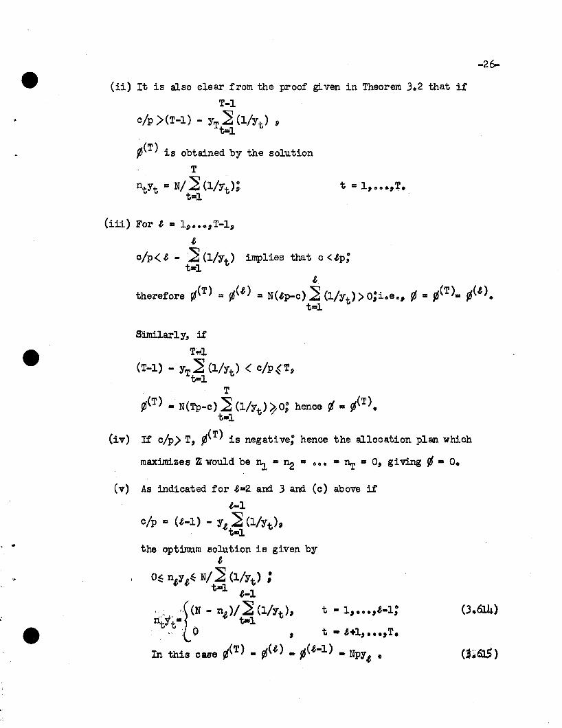
(ii) It is also clear from the proof given in Theorem 3.2 that if
T-l
c/p )(T-l) - YT·~ (l/Yt) 9t-l
¢(T) is obtained by the solution
T
ntYt - NI~ (l/Yt);t-l
(iii) For t ... 1~•••~T-19
tc/p<t -~(l/Yt) implies that c<.ep;
t-lt
therefore fi(T) = ¢(t) = N(.ep-c)~ (l/Yt) >O;i.e., ¢ • ¢(T). ¢(.e).tal
$iJnilarly, if
T~l
(T-l) - YT~ (l/Yt) <c/p(T,tal
T'¢(T) ... N(Tp-c) ~ (l/Yt) ~O; hence fi _ ¢(T).
tal
(iv) If c/p) T, ¢(T) is negative; hence the allooation plan whioh
maximizes ~ would be Il:L - ~ ... 1)0. =- ~ - 0, giving ¢ - O.
(v) As indioated for t-2. and 3 and (c) above if
t-l
alp ... (.e-l) - Y.e ~ (l/Yt)'t-l
t ... 1, •••,.e-l;
wi the optimum solution is given by.e
O~ n.eYt!:: NI~ (l/Yt) :tal t-l
.;.;.. c'[(N - n.e)1~ (l/Yt),rliit-. t-l. ,~O , t • .e+l, ...,T.
In this ease ¢(T) - ¢(t) _J6(.e-l) -NPY.e 0
(3.61.4)
'...
-27-
307 summary
In this section we have analyzed a simplified model to illustrate
some basic characteristics of the pnofulemo The optimal allocation plans
were obtained for every value of c/p in the interval c/p)Oo This
interval was divided into (T+I) sub-intervals, in each or which an
explicit optimal solution was obtainedo Given c, p and Yt (t = 19 0 oo.\lT)
one can easily find the appropriate sub-interval and thus the optimal
allocation plano These results are presented in Table 301 The simpli
fying assumption that the firm is concerned with the optimal allocation
of a single resource made it possible to obtain the above results with
the analytic tools used o However, for studying the more realistic and
thus more complicated model formulated in Section 2 0 3, we will need a
set of analytic tools more powerful and flexible than "lhose used in
analyzing the simplified modelo The methods of linear programming pro
vide us with such tools o
e.. ~
e
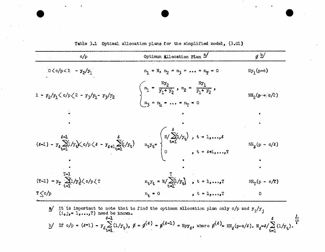
Table 3.1 optimal allocation plans for the simplified model, (3.01)
e
c/p
0< c/p<: 1 - '12/'11
1 ~ '12/'11< c/p<2 - '13/'11- '13/~2
..•
optimum Allocation Plan !I
~ • N, ~ - n3 • ... • Dr .... 0
NY2 Ny!n.. ,n..= ,
.L '11+ '12 .. " Yl+ '12
""~ • ~ • 0
!l
•
¢!¥
NYl(P-c)
NH2(p-,e,/O/2)
•
"
t~ t
(t...l) - Yt~l/y'J<c/p<t - Yt+l~~/Yt)tel tal
•
"
ntYt-
t
N/ ~~/Yt) ~ t '. l, ...,~tal
, t • t+l, ••• ,T
••
NH~(p ... cit)
••
T-l
(T-l) - YT'~l/Y~(C/P<Ttal .
TS;c/p
T
nt'1t - N/~~/yJ ' tal, oe .,T. tal
nt - 0 , t • 1,.oo,T
NHT(p - cil')
o
!I It' is important to note that to find the optimum allocation plan only c/p and y. /'1.(i,j,. 1,,, ••,T) need be known. ~ J I
t~ . t NCXl
2/ It' c/p u (t-l) - '1e.~ (l/Yt)" ¢ - ¢(t) == ¢(t-l) =NPYt , where ¢(t). NHt(p-clt). HtUt/~ (l/yt). •
t-l." ,.. tal
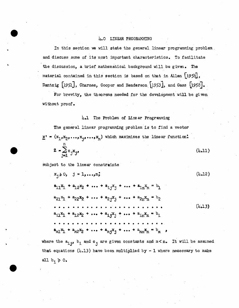
4.0 LINEAR PROGRAMMING
In this section we will state the general linear programming problem.
and discuss some of its most important characteristics. To facilitate
the discussion, a brief mathematical background will be given. The
material contained in this section is based on that in Allen [1956],
Dantzig (195J.], Charnes, Cooper and Henderson [1953], and Gass [1958J.
For brevity, theth eoreins needed for the development will be givan
without proof.
4.1 The Problem of Lire ar Programmirg
The general linear programming problem is to find a vector
Xl .. (xp~,••• ,xj ' •••,~) which maximizes the linear function:
n
z: .~c.x.,j=l J J
subject to the linear constraints
X j ~ 0, j =1,.. ••,n;
(4.11)
(4.12 )
+a..x. +~J J
+ a2··x . +J J
• • • • • • • • • • • • • • • • • •. • • 0 ••• (4~3)
+ a. x = b.mn J.
4
• • • • • • • • • • • • • • • • • • • • • • • •
where the aij, bi and c j are given constants and m<n. It will be assumed
that equations (4.13) have been multiplied by - 1 where necessary to make
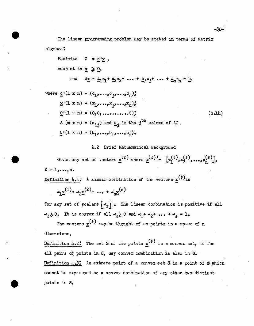
The linear programming problem may be stated in terms of matrix
algebra:
Maximize Z a ~t! ,
subjeot to ! ~.Q,
and ~ a ~x.t+ !2~+ ... + !jXj + ... + ::'n~ a ~,
where ~t(l x n) a (Ol, ••• ,Oj, •••,On);
!'(l X n) a (x:!.' ...,xj ' ...,Xn );
£1(1 x n) a (O,O,o ••• ~ ••••••O);
A (m::x n) a (aij ) and !oj is the jth oolumn of A;
~'(l x n) a (bl, •••,bi, •••,bm).
4.2 Brief Mathematioal Background
(4.l4)
Given any set of veotors x(.e) where x(.e) 'a rx.,(.e) x1.e} x(.e}lGJ. ,--~ , ... , n J,
.e = l, •••,s.Definition 4.1: A linear oombination or the veotors x(I)is
for arry set of soalars [-":e]. The linear oombination is positive if all
"".e~ O. It is convex if all "".e~ 0 and -<:t+ ""2+ ... + ""s a 1.
The vectors !(.e) may be thought of as points in a space of n
dimensions.
FIefinition 4.2: The set 5: of the points !(.e) is a convex set, if for
all pairs of points in S~ any convex combination is also in S.
Definition 4.3: .An extreme :point of a convex set a is a point of S which
oannot be expressed as a convex combination of arr:r other two distinct
points in S.
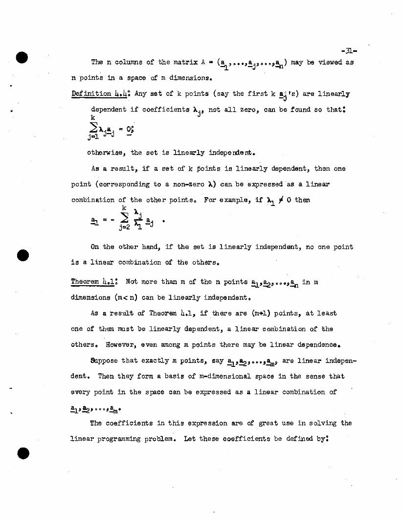
-31The n columns of the matrix A = (a p ..,a.,o ... ".~,.J may be viewed as
~ -J -n
n points in a space of m dimensions.
Definition 4.4: A.ny set of k points (say the first k a-l IS) are linearly-J
dependent if coefficients A., not all zero, can be found so that:k J
] Aj.a
j= 0;-
j=l - -
otherwise, the set is linearly indepen:ient.
As a result, if a set of k points is linearly dependent, then one
point (corresponding to a non-zero A) can be expressed as a linear
combination of the other pointso For example, if Al r! 0 thenk A
!J. =- j~ it!j ·On the other hand, if the set is 1 inearly independent, no one point
is a linear combination of the others.
Theorem 4.1: Not more than m of the n points !;J..'!:2,ooe"!n in m
dimensions (m< n) can be linearly independento
As a result of Theorem 4.1, if there are (m+l) points, at least
one of them m:u.st be linearly dependent, a linear combination of the
others. However, even among m points there may be linear dependence.
Suppose that exactly m points, say .!J..,!2," ""!m' are linear indepen
dento Then they form a basis of m-dimensional space in the sense that
every point in the space can be expressed as a. linear combination of
The coefficients in this expression are of great use in solving the
linear programming problem. Let these coefficients be defined by:
a. = a.. x.. . + a...x..- .+-J ~-.LJ .-r::Ui:::J ••• .. a. x..+ ••• + ~X • ,-~ ~J ~.. InJ
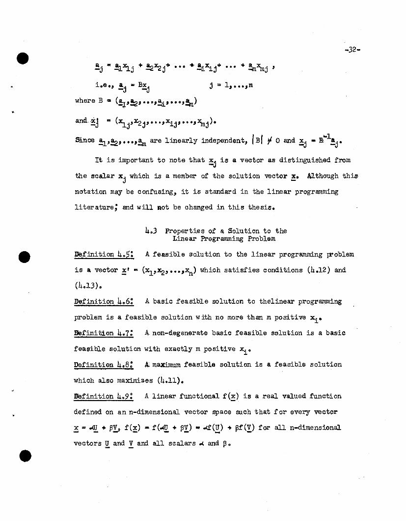
-32-
i.e., a. = Bx.-J -J
where B • (~'!2, •••,:a' ...'!m)
and;oc!-J
j .. 1, ...,n
It is important to note that !j is a vector as distinguished from
the scalar x j which is a member of the solution vector!. A.lthough this
notation may be confusing, it is standard in the linear programming
literature; and will Rot be changed in this thesis.
4..3 Properties of a 50lution to theLinear Programming Problem
Definition 4.. 5= A feasible solution to the linear programming p:oblem
is a vector Xl = (X1'X2' •••'~) which satisfies conditions (4.12) and
(4.13)&
Definition 4.6: A basic feasible solution to thelinear programming
problem is a feasible solution with no more than m positive ~.
Definition 4.7: Anon-degenerate basic feasible solution is a basic
feasible solution with exactly m positive Xi.
Definition 4&S: kmax~ feasible solution is a feasible solution
which also maximizes (4.11).
Definition 409: A linear functional f(!) is a real valued function
defined on an n-dimensional vector space such that f or every vector
25 := -<! + ~L f(!) = f(-4!L + ~!) == -d<!!) + ~r(!) for all n-dimensional
vectors U and V and all scalars .( and ~ &
-33-Note that the objective function (4 ..11) is a linear functional for
those ~ satisfying (4.12) and (4,,13).
Theorem 4.2: The set of all feasible sOlutions to the linear programming
problem is a convex set.
we shall denote the convex set of the feasible solutions to the
linear programming problem by r. Since r is determined by the inter
section of the finite set of linear constraints (4.12) and (4,,13),
it can either be void, a convex polygon, or a convex region which is
unbounded in some diJioectiono If' r is void, the problem doe s not
have any sOlutions; if it is a convex polygon, the problem has a
solution with a finite value for the objective function; and if r
is unbounded, the problem has a solution, but the maximum :might be
unbounded. If' r is a convex polygon, it has a finite number of
extrema. points and every feasible solution in roan be represented
as a convex oombination of the extreme, feasible solutions in r.
An unbounded r also has a finite number of extreme points but not
all points in r can be represented as convex combinations of these
extreme points. For computational purposes r is assumed to be a
convex polygon.
Theorem 4&3: The objective function (4,,11) assumes its maximum at an
extreme point of the convex set r generated by the set of feasible
solutions to the linear programming problem. If' it assumes its maximum
at more than one extreme point, then it takes on the same value for
every convex combination of those particular points o
As a result of Theorem 4.3 we need only look at the extreme
points of r in order to determine the maxinn.lm feasible solution~
Theorem 4.4:-34-
If a set of k~ m vectors .=a"!2'. ""!k can be f!ound that
are linearly independent and such that
and all xi~ 0, then the point ~' = (Xi"x2' ••• 'Xk,0, •••"O) is an extreme
point of the convex set of feasible solutionso
Theorem 4.,:the vectors associated with positive X1 form a linearly independent set.
From this it follows that" at most, m of the xi are positive.
Yiithout any loss of generality the set of vectors ~, ".'!n
can be assumed to contain a set of m linearly independent vectors.
If this is not evident when a particular problem is being solved,
the original set of vectors is augmented by a set of m linearly
independent vectors and a 13 alution to the extended problem is
sought.
Clfurollary: Associated with every extreme point of r is a set of
m linearly independent vectors from the given set ~,~, •••'!n.
The preceding theorems may be summariz~d by the following:
Theorem 4.6: .!' = (Xi"X2' oe og~) is an extreme point of r if and only
if the positive x j are coefficients of linearly independent vectors in
n
~ &;XJ
9 "" b •j=l-u -
From the assumptions and theorems of this section we can conclude
that only extreme points need to be investigated and thus we can l:i.mit
our search to those solutions which are generated by m linearly indepen-
dent vectorso There are a: finite number of such solutions since there
-35-are at most (:) sets of m linearly independent vectors from the given
set of n. However for large n am m it would be almost impossible to
evaluate all the possible solutions and choose the one which maximizes
the objective functiono
The simplex procedure, devised by G.. Bo Dantzig [1951J finds an
extreme point and determines whether it is the maximumo If it is not"
the procedure finds a neighboring extreme point whose corresponding
value of the objective function is greater than or equal to the pre
ceding value" In a finite number of such steps (usually between m and
2m) a maximum feasible solution is found o The simplex procedure makes
it possible to discover whether the problem has no finite maximum
solution or no feasible solutions ..
404 The Simplex Computational Procedure
Assume that the linear programming problem is feasible, that every
basic feasible solution is non-degenerate and that a basic feasible
solution is given. As will be seen later these assumptions are not
restrictive.. Let this given solution be ~ "" (~.lI~~ 0 ooSlJCln), where
the zero elements have been deleted from ~ and the associated set of
:llJ.!:.L + ~!:! +
and :;,~ .. ~c2 +
000
000 +xc ""Z:O.1lmm
(4 .. lU)
(4042)
where all xi> O. In matrix notation1l these can be written as
-36-
In order to determine if Max Z, = ~O we need to determine the change
in Z as a result of replacing ~ by some other extreme point solution.
The simplex method does this by determining the sign of the change in Z
resulting from the replacement Of !o by anyone of the neighboring
extreme point solutionso This is accomplished without computing these
neighboring extreme point solutions.
Suppose we introduce Q units: of one of the variables, say the jth
one.!> whose corresponding vector is not in Bo The solution ccntaining Q
units of the variable j has to fulfil the linear constraints (4012) and
(4013) in order to be feasible o
As a result of introducing Q units of variable j, let the variables
XJ.Sl~.!> 000.!>:Jtn be changed to JIl- QJIlj9~"'-Q~j"H.9:Jtn-Q:Jtnj' respectively,
or in general !o is changed to ~ em Q.!j' where !j = (JI1.j'~j' 0& O.ll~j).
To satisfy condition (4013), x. must be chosen SUch that-J
B [!Co Q!j] ... Q!j =£; j'" M+l.!>ooo»no (4044)
Since B is non-singular and in order to satisfy (4044), x. is g1ven by-J
[ =1 ~ I =1 -1x. "'" B b... Ie ... B a .... B a. 0
-J - -J-J Oh45)
To satisfy condition (4012),1) Q must be such that ~.... Q!j?.Q.
ioe o.!> :x:t "" @Xij~ 0,1) ~ ... @~j ~ 090" °9Xm ... @:Jtnj ~ 0 0 (4046)
Given x. as in (4045) and some Q Which satisfies (4046), the change in-J
Z will be
where
(4049)
If for a fixed j.9 c. = Z.• >0 and some Q) 0 satisfying (4046) canJ J
be found» then the new Z. will be greater than ZO° This leads to the
follow:ing theoremo
Theorem 40n If for any fixed j the condition c j - z,j> 0 holds,9 then
a set of feasible solutions can be constructed such that Z>Zo for any
member of the set where the upper bound of Z is either finite or
infinite 0
mase.I: If finite,!) a feasible solution consisting of exactly
m positive variables whose value of the objective function is
greater than the value for the preceding solutiono
Case II~ If infinite, a feasible solution consisting of
exactly m .. I positive variables can be constructed where the
vvalue of the objective function could be arbitrarily large"
Since Xi> 0 for all i in (4046),!) it is clear that there is for
@}O either a finite range of values @j)@)O or an infinite range of
values such the xi = @Xij.9 i "'" l,9a.9 ""0.\lm.\l remain positiveo It is clear
from the assumption in the theorem that for a fixed j» cf" Z:j> 09
Z § Zo .. @(cj = z,j) is a strictly monotone increasing function of @o
~se I: If for a fixed j with c j = Z:j> 0 at least one Xij ) 0 in
~;__l (4 ..45) and (4046)$) for i "'" 1.fi2.\l 00 0.\lm$) the largest value of @ for
which all elements (xi = @~j) remain positive is given by
Q. ... Minf ; 1)1 0 .fiJ i Lij
.•
If i ... i. yields @'J) it is clear that the variable corresponding toJ J
i l;;l i. in (4046) will vanish; hence» a new feasible solution isJ
obtaine4> consisting of Qj and (m-l) of xi"" @jXij; i=l,90oo»mg i I if"
A new basis is obtained consisting of a. and (m-l) of the m-J
vectors previously used o With this basis, we can perform a new set
of computationsJ) as above.
If' a new cj'" Zj> 0 and a corresponding xij>O,\) another solution
can be obtained with a greater value of Zo This process will con-
tinue either until all cj"" Z;j~ 0, or untilJ) for some c j"" Z;j> 0,9
all x ..~ 00 If all c.= Z" >O,\) the process terminateso~J J J
case II: If at any stage for some j.\l Cj
"" Zh> 0 and all x .. ~ 0,J . ~J
then there is no finite upper boundll and for any Q> 0 all elements
of (4046) are positive; hence a feasible sOlution consisting of
m+l positive xi is obtained o Therefore by taking @ large enoughg
the corresponding value of the objective function~Z: = ZO+ Q(cj"''' Zj)
can be made arbitrarily large o
Theorem 4,,8~ If for any basic feasible solution ~ "" (:x:t.\l0 OOSlXm) the
condition c j = Zj6-0 holds for all j "" 11l000.\lnll then (4041) and (4042)
constitute a maximum feasible solution"
The results of Theorems 406 and 4,,8 enable us to start with a
basic feasible solution and generate a set of new feasible solutions
that converge to the maximum solution or determine that a finite
solution does not existo The non=degeneracy assumption was made to
insure the convergence to the max:i.muln solutiono W'iithout this
assumption,\) the procedure can conceivably repeat a basis and hence keep
-39-
returning to the same basis. The s:ilnplex procedure is then said to have
cycled, and the computational routine for determining the maximum
solution breaks down.
However, Dantaig, Orden and Wolfe (1954J and Charnes, Cooper and
Henderson (1953] have resolved degeneracy from both the theoretical and
computational points of view, using the basic ideas of the s:ilnplex
procedure" This "makes the simplex method available without blemish as
a crisp tool for proving pure theorems," Hoffman [1955].Dantzig (195Y points out that the number of iterations needed to
obtain a maximum feasible solution is expected to be greatly reduced
not by arbitrarily selecting any vector a. satisfying Zj< c. to be-J J
introduced in the basis, but by selecting the one which gives the
greatest immediate increase in Z.
one which corresponds to
The vector a. should thus be the-J
~x Qj (c j - z,j)J
Where for each j, ~. := Min lXi ~ >o.J 0 x..~ ~J
A criterion which involves considerably fewer computations, and
which has proved to bean excellent one is to select the vector which
corresponds to
Max(c.- Z:j).j J
-40-4.5 The Dual Problem of Linear Programming
Associated with every linear programming problem as stated in
section 4.1 is a corresponding optimization problem called the dual
problem. The original problem is termed the primal. The primal is
stated as in Section 4.1, i.e.,
Find! which maximizes ~ =~'! subject to the linear constraints:
!~o2
am A! = E"Where ~, ~, A, 02, b are defined· in (4014). The associated dual
problem is:
Find :!i(mxl) which minimizes V =£':!i subject to the linear .
constraints:
AI!~~o (4.52)
In the dual problem the variables up i =1, •• ",m, are not restricted
to be non-negative. However, if the restrictions in the primal are
written A.! ~ E" the variables ui in the dIal are restricted to be non
negative.
The importance of the dual problem can be seen from the following
theorem known as "The Duality Theorem."
Theorem 4.9: If either the primal or the dual problem has a finite
optimum solution, then the other problem has a finite opt:innlm solution
and the extremes of the linear functions are equal; i.e o , Max Z:: = Min V.
If either problem has an unbounded optimum solution, then the other
problem has no feasible solutions.
..
e-, .0 USE OF L:lliEAR PROGRAMM:lliG PROCEDURES FOR
THE PRODUCTION STABILIZATION PROBLEM
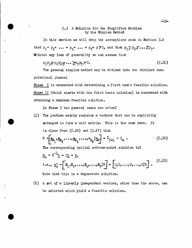
In sections '01 and , ..2 we will :r;resent a linear programming formu.-
lation for the general and s:implified production stabilization problems.
In section '03 a solution will be given to the simplified :r;roblem using
the simplex method o In this we will not assume as in (3.01) that
Pl = P2 = 0 •• =Pi = 000 = PTo A useful initial basis will be suggested
in Section '04 for starting the iterative procedure of solving the general
production stabilization problem o A criterion for selecting the vector
to be introduced into the basis will be given in Section '0'. The
properties or the initial basis suggested in section '04 and the criterion
suggested in Section ,., will be used in Section ,.6 to obtain the optimal
solution to the general production stabilization problem, associated
with each value of the cost parameter c in the interval c~Q;.
'01 A Linear Programming Formulation ofthe Production Stabilization Problem
Recall that our objective was to find the allocation plan:
subject to the constraints~
T
~t ,?O and t~nrt~Nr ;
('oIl)
(,012 )
.. (,.13)
-42-.f
Let Gt = ~ nrtYrt = total output in time period t"
and G* = !lax r:-J1 = !lax r] '\-1yr1' ] '\-2Yr2' ..., ] "rTYJ.t L &=1 r=l r=l ~
The variable G* has the following relations with the other variables:
f
~nrtYrt - G*~O;r=1
t ... l" ..."T • (5 o~5)
Hence if we include (5.15) among the:restrictions on the allocation
variables, the problem is restated as:
Maximize the linear objective function
f T
~ ~ ~YrtPrt - c G*"r=l t=l
subjeot to the linear inequalities
Ilz-t~ O;G*~ 0;
(5.16)
Let
T
t~Ilz-t"!:-Nr ,,
f
Et "" G* - ~ Ilz-tYrt ~ 0"r=l
r =l" ..."f.
t ... 1" •••"T,
(5018)
(5.110)
T
and D'r == Nr - ~~t ;;'0,t=l
r ... 1" •••,f. (5.111)
We oan now state the problem in the general linear programming form
given in Section 4.1 as follows:
-4.3-
Find the vector:
[!1, ...,~;Dl,.·.,Df;"21"··'"2T;"';~1"·"~T;.··;nfl'.·"nfT;G:J(,.112)
which maximizes the linear objective function
subject to the l:inear constraints:
(,.113)
f
and Et + ]nrtYrt - G* = 0,r=l
r=l, •••,f;t=l, ••• ,T,
tal, oe .,T;
T
Dr + t~nrt == N,r r=I, •••,f. (5,,116)
Note that the number of variables: n = T + f + Tf + 1 ... (T+l)(f+l);
and the number of constraints: m ... T + f'<; n.
,.2 A Linear Programming Formulationof the Simplified Model
If there is only one resource that could be channeled to yield an
output in time periods t ... 1,2, ••• ,T, the problem can be stated in the
general linear programming form as follows:
Find the vector !' =[El' ooo'ET;D;~ ..~, o..,nr;G*] ,which maximizes the lirear function:
T Tz: ... 0]Et + OD + ] ~YtPt - c G* ..
t=1 tal
-44-subject to the linear constraints:
It ?,o;uz O;nt ~ O;G*~ 0,
*and Et + ntYt - G = 0, t=l~...,T;
T
D+~ut=Not=l
For this simplified model the number of variables:n = 2.(T + 1); and the
number of constraints: m = T + 1.
I -1 E1 0, \_,
--I E 01-1 2f, 0 .. 0
I-1 Et, 0,, .. .. - ..,
1-1 ET 0,;- - -
0 D N
~
~
..nt
0
~
G*
o
"
o
o
o
•
•
•
It
•
o
..
It
o
Y1 0 • 0
o Y2 It 0
Constraints (,.24) and ('02,) may be stated in matrix form:
I I•
• 0.0 10 1• I,
.0.0 '01, I,
• • • • ,. I •, I
.' 1 • 0 ~ 0: 0 0 .. Yt" 0, ,• .. • • '. I •
l I~ 0 • 1 I 0 I 0 0 • 0 " YT
, I-,-t----~ 0 .0,1,11 _,1.1o 0
1 0
0 1
• •
"0 0
• •
0 0
The column vectors of the matrix A maN' be identified
A • [.'!&.t'~l :~!!Et' "!!&r:.:n:~.~•.•" •.•~:~] •as follows:
5.3 A Solution for the Simplified Problemby the Simplex Method
In this section we will drop the assumptions made in section 3..0
that Pl= P2= .... = Pt= ... = PT= p'O, and that Ylt. Y27, .. • 'ZYT"
Without any loss of generality we can assume that
(5.31)
The general simplex method may be divided into two distinct com-
putational phases:
Phase I is concerned with determining a first basic feasible solution"
Phase II (which starts with the first basic solution) is concerned with
obtaining a max:i.m.um feasible s elution.
In Phase I two general cases can arise:
(1) The problem matrix contains m vectors that can be explicitly
arranged to form a unit matrix. This is the case here. It
is clear from (5.26) and (5.27) that
B Dr:~'!E2' •••'!Et' •••'~;~ DIT+1 = 1m • (5.32)
The corresponding initial extreme-point solution is:
x =B-~ = Ib == b.~ - - -"
i.e., !6 ==[~,E2'''' .,Et , H o'E.r;~ == ~,o, I>U,O, u.,O;N] •
Note that this is a degenerate solution..
(2) A set of m linearly independent vectors, other than the above, can
be selected which yield a feasible solution.
-46-
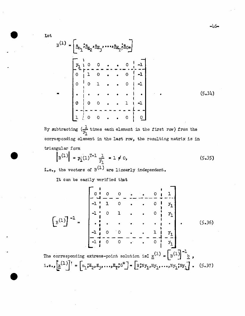
Let
\!
Yl \ 0 0 • • 0 , -1_. r- - - - - ----_ .. _--
0 I 1 0 0 r -1• ..I
0 I 0 1 0 I -1• ..I I
= I I (5.34)• I • .. • • • • •I I
0 I 0 0 • • 1 \ -1I _ L _
- -1- - - - - - - - - -I I
1 I 0 0 .. .. 0 I 0l,
By subtracting (..l times each element in the first row) from theYl
corresponding element in the last row, the resulting matrix is in
triangular form
IB(l)1 = 7i(1)T-l ~ • 1 , 0,
i.e., the vectors of B(l) are linearly independent.
It can be easily verified that
(5.36)•~(l~ -1 =
I
0 1 000 .. 0 1- -.I _ - -- -- -- - or ----
-1' 1 0 .. • 0' YlI ,
-1" 0 1 .. 0 0' y.I , 1• I
-0 I 0 .. .. 0 "I ..I l
-1, 0 ' 0 .. .. 1 I Yl- -11---- --I-1: 0 0 .. .. 0: Yl
The corresponding extreme-point solution is: !(l) =[B (l~ -1£ ,
i.e., ~(lj ~ = [~;E2,E3'." .,ET;G*J =~;NYl'NYl' ••• ,NY1;NY1] ..
-47-Note that this is a non-degenerate basic feasible solution. We will
start Phase II with the initial basic feasible solution given by (,.37) •
.Also note that here we prefer the notation x(l) instead of x , because- -0
of its connection with the number of time periods used.
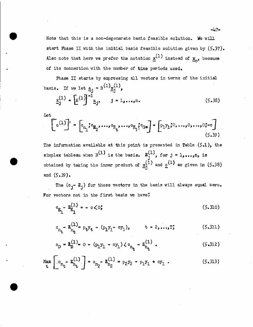
Phase II starts by expressing all vectors in terms of the initial
basis. If we let a. =B(l)x~l),-J -J
x(.l) = CB,(ln -la .-J ~ ~ -J' j =1, •••,n.
Let
[0(1~1 • rn/'B:1' ...."Et....."E.r~OGit]. [PJ.Yl;O, ••••0••.••0;-oJ
(5.39 )
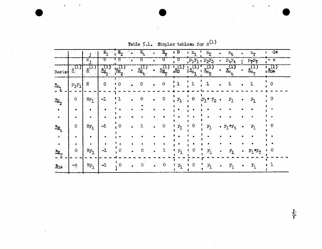
The information available at this point is presented in Table (,.1), the
s:ilnplex tableau when B(l) is the basis. Z;~1), for j = 1, ... ,n, is
obtained by taking the inner prcxluct of x~l) and c(l) as given in (,.38)-J -
and (,.39).
The (c j - ~j) for those vectors in the basis will always equal zero.
For vectors not in the first basis we have:
c - Z'11) = - c<o;El J!i1
t = 2, ...,T;
(5.310)
(,.311)
(, .312)
(,.313)
e e
Table 5.1. Simplex tableau for B(1)
(
e
j . .E1 ·: .E2 ... • ·E.t • 'E.r ~ D ~ 11. : ~ • nt • ~ 'G*
C j e : e • () • 0 ,0 ,P1Yl' P'2Y2 • PtYt : PTYT ,- 0
. otlJ xtl) ~..lIJ ,xS..~.1.J. • xi.I. .J. • ~.,(I.. J 'xilJ Ixtl) I x(1) • x(1) .. Xt1.,) '~:)Bas~s - - -~-'~2 ""'llI.it , ,-Jj ,~' -~ -llt -~ 'OOJ,j'R, . , , , ,a P1Yl N 0 '0 • 0 • 0 ,I 1,1 • 1 • 1 0-~ , ' ,- - - - - - - ~ - - - - ~ ~ - - - - - - - - - ~ ~ - - ~ - - 1- _ _ _ _ _ _ _ _ _ _ _ _ ~ _ _ _ _, , , , ,~2 0 NYI -1 : 1 • 0 • 0 ,11' 0 ,11~ ¥'2· Yl • Yl ,0
'II ", I• ' 0 .. ,. ,. , 0 ,0
· : '. '. ' '.I , , I
I I.!E 0 NYI -1 , 0 • 1 • 0 '11' 0 Yl. Yl+Yt • Yl I 0t I , ' ,, ,
• • 0 • , ••••• '. ' •• 0" •• I.I , I ,• ••• ' ••••• ,II ,. , ...... ,.
!J!: 0 NYl -1 : 0 • 0 • 1 '11' 0 I Yl • 11 • 11i'YT ' 0T , , ' ,- - - - - - - - - - - - ~ - - - - - - - - - - - - ~ - - - - r - - ~ - - - - ~ - - - - ~ - - ~ -, ' , ,!Q..i~ -0 NY1 -1 lOco 0 • 0 'Yl' 0 'Y1 • Y1 • Yl ,1
I , , , ,
I.I:='"'
'f
-49-If (5.313) is non-positive, the solution given in (,5.37) is a final
.. solution with the corresponding value of the objective function:
~(l) =NY1(Pl-c)' (5.314)
Since P2Y2 - P1Yl of; cYl~O implies (Pl-c),?P2Y2/Yl> O,,-z.,(l).>,C i£2'5(l) is
a'maxinn.un:s.oluti'on.
If' P2Y2 - P1Yl + cYl70, !~ is introduced into the basis" The
vector to be eliIninated from the basis is the one corresponding to:
Mini
(5.315)
(5.316)"
~ rows
J, -1
, -1,1 "I, -1o
"o 0 " 1~' 0 0 "- - - - - - - -f- - - - - - - - -t- -
therefore,!E is eliminated from tl:'e basis.2
The second basis is B(2) =[ ~'!n2;.!:E3' ."'!ET;!o.J.
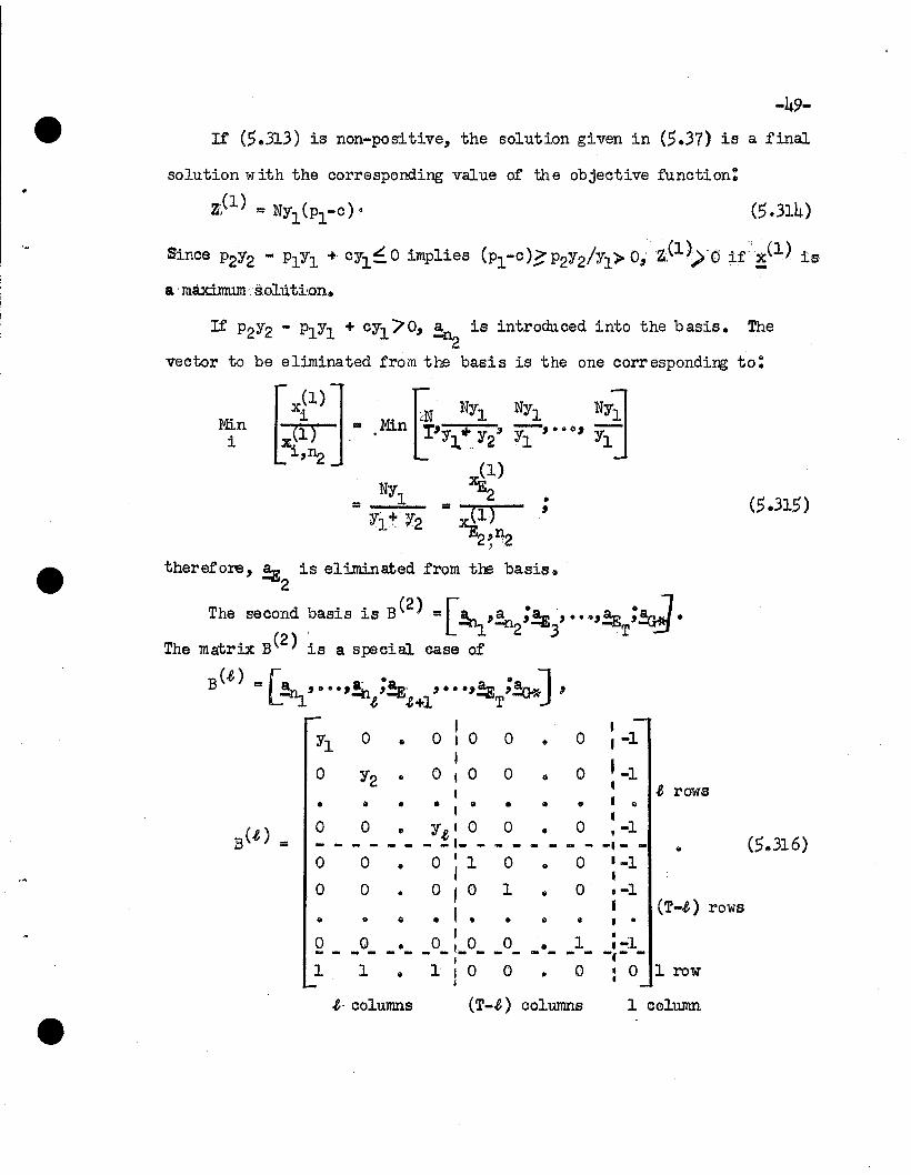
The matrix B(2) is a special case of
B(.t)-[ -" .. J- ~" ".. '!n,!E ' "",~,,~ ,~1. ~ $+1 T
o .. 0: 0 0 " 0I
12 " 0 I 0 0 " 0I
" • • I" " " "
0 0 0 I 1 0 0 1-1• I ••0 0 • 0 I 0 1 " 0 • -1
I I (T~) rows" • " " " • .. .. • •0 0
I1 •
" 0-'-0 0 It .-1-- - - - -- - - - - - - - -,- -I1 1 " 1 I 0 0 " 0 0 1 row
I
:e. columns (T-:e) columns 1 column
I I_ K(~)
I 0 0 • 0f K(~)
Y1Y~ I I Yl• I
_ K(~) ,0
IK(~~, 0 0 • I
Y2Y.e ,I Y2,
•
•
1~
~ (l/Yt)tal
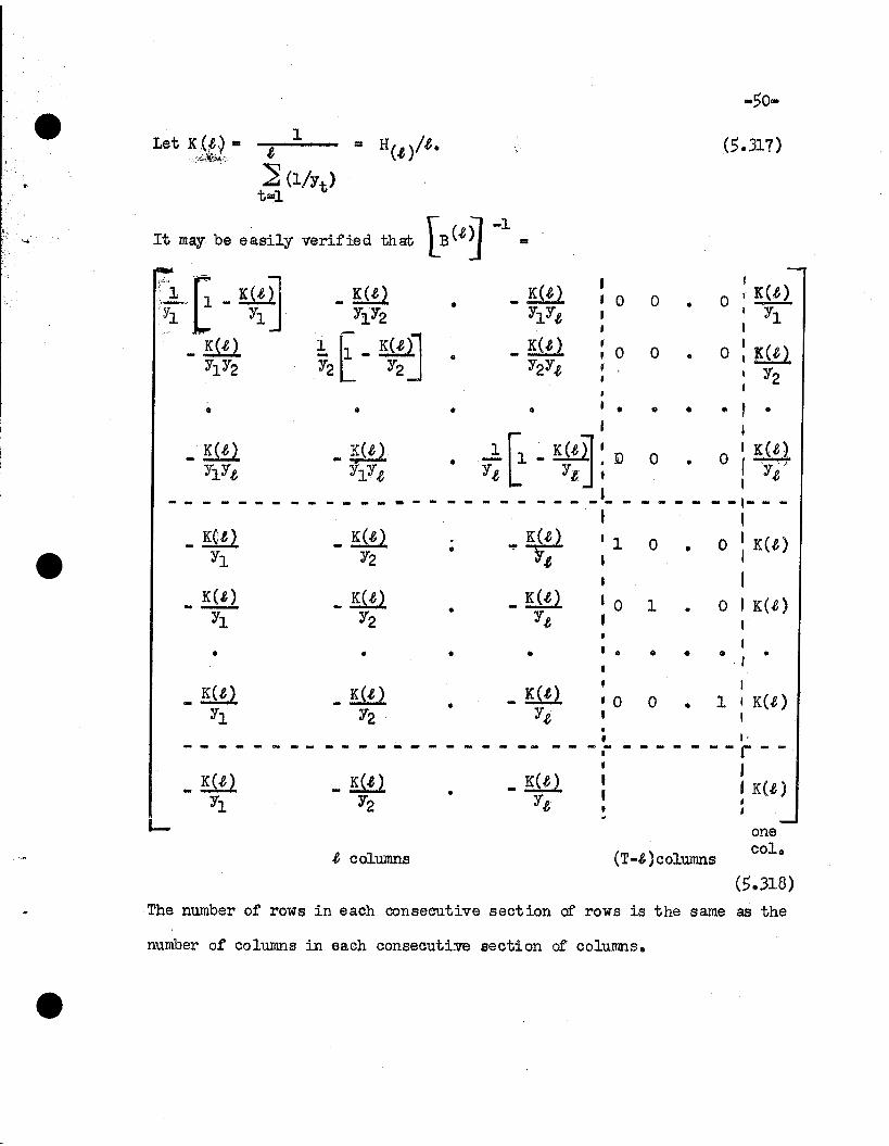
It may be easily verified that [B(~~ -1 =
Let Kte,~ a.--.:_&.~~;.
••
K(.e ).,. Y.e
_llily~
•
•
·•
•
•
•
•,I. • • • I •I I
• ..!. [1 -K(.elf ~ DO. 0I K(.e~Y~ Y:e:J' f Y.e'
I- - - - - - - ... - - - .. - - - -- - - - -- .. - -- -,-- - -I
1 0 • 0: K(~)
Io 1 • 0 I K(~)
1I
• • • • , I
1o 0 • 1 I K(~)
I
•
-,'.
-------
•
onecol.
II K(~)j
j
I'---------j--
(T-~ )colunms~ columns
- - - -- .. - .. -- - - .. - _.. --•,,,,~
(5.318)
The number of rows in each consecutive section of rows is the same as the
number of columns in each consecutive section of columns.
-.51-
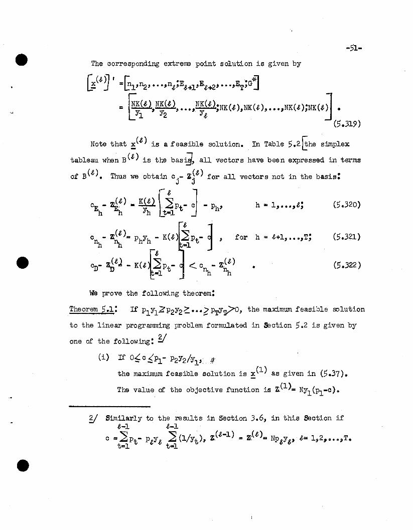
The corresponding extrellB point solution is given by
[~(.e~ t =Gl'~' •••"n.e;E.e+l'E:e+2" ••• ,ET;Gj
= ~~~t).N~~t)•••••N~;t);NK(t).NK(t)""'NK(t);NK(tiJ•(.5.319)
(5.322 )
(.5 ..321)
(.5 ..320)h = 1" • ..".e;
•
Note that !.(.e) is a feasible solution. In Table .5.25he s:iJnplex
tableau when B(.e) is the basil, all vectors have been expressed in terms
of B(.e). Thus we obtain c.- Z;~.e) for all vectors not in the basis:J J
"E - ~t) = K(t) r~Pt- J-Ph'h h Yh hal J
C - z(t)= PhYh - K(t) ~Pt-]' for h = t+1• ••••~;~ ~ =1 J
"D- ~(J. - K(t{ipt- <. C'1,.- z;~)
We prove the following theorem:
Theorem .5.1: If P1Yl,ZP2y2-2: ...ZPTY~' the maximum feasible oolution
to the linear programming problem formulated in Section .5.2 is given by
one of the following: Y(i) If O~ c .{Pl- P2Y2!YV {!
the maximum feasible solution is !.(l) as given in (.5.37).
The value of the objective function is ~(l)= NY1(Pl-C).
Y Similarly to the results in Section 3 .. 6, in this Section if.e-l .e-l
c =~Pt- P.eY.e ~(l/Yt), Z;(.e-l) = z:(.e)= NP.eY.e" .e= 1,2, .... ,T.tal tal
e e e
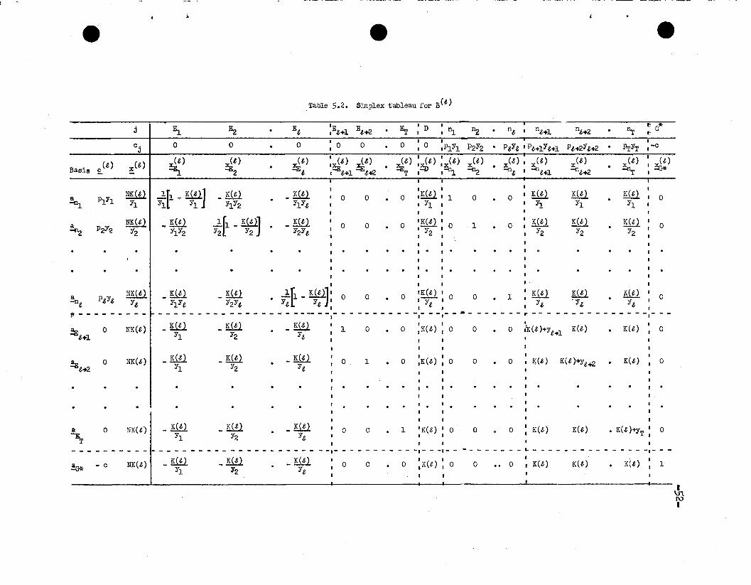
Table 5.2. Simplex tableau for B(t)
~t PtYe NK(t)Y
~-------~-
j
-~
Basis £,(t) x($)
a NK(~)
-D1P1Y1 Y1
a NK(t)
~ P2Y~ Y2
~NI
o
o
, 0
••1 •
I
••
K(e)
K(t)Ye
K(e)
~ .' G*.',PrYT -c1
(e) 1 (e)~~ '~
1
i1
K(e) , 0Y1 ,
1
K(e) : 0Y2
• K(e)+YT: 0K(t)
K(e)Y1
K(e)'Ye
K(e)
Y2
K(t)Y2
K(e)Ye
K(e)
Ylo
o
1o
o
o
o
1
o ,K(t) K(t)+Ye+2I
I
I,I,,
o : K(t)
I 1-- - - - - - - .. - - - - - - - - - - - - - - -,- - -, . 1
o •• 0 I K(t) K(e) • K(e) 1 1,
I
1 •
1,1 1I ,
1 IK(e) 1 0, ,1 ,
- - -,- - -1- -, ,o ,K(e) 1 0
Er I D ,ne+21
, n1 ~ · ne, ne+1
1 0 1,
01 IP1Y1 P2Y2 · PeYe I Pe+1Ye+1 Pe+2Ye+2 .
~e) :~e) :x(e)1. x(e) · x(e) I x(e) x(e)
Til"""). -~ -Dt I -ile+1 -De+2--,----- ---------
o
o
o
o
o
1
o
o
1
1
IEH1 Ee+2
, 0 01
:~e) ~t)1 e+1 e+2T
1
, 0
1
11 01
•I •
1
1
I,, 0•1- -,- - - - - - - -
o
(e)~t
Ee
_ K(e)Ye
K(t)- Ye
_ K(e)Ye
_ K(e)Ye
_ K(e)
Y2Ye
_ K(e)Y1Ye
o
E2
(e)
~2
_ K(e)
Y2
_ K(t)
Y2
_ K(e)
Y2
K(e)- Y2Yt
_ K(t)
Y2
_ K(e)
Y1Y2
.1:.f1 _ K(e )]Y2[ Y2 ]
oEi
~)
K(e)-Yl"
_ K(e)
Y1
_ K(e)
Y1
_ K(e)Y1
_llllY1Ye
K(e)- Y1Y2
1 1o ,K(e) I 1
'Y1 11 ,
IK(e) ,o 1 Y I 0
1 2 1
1 1I· ,.
I I
'. '1 1, ,
.1:.f1 _ K(e)} 0 0 0 IK(e) 1 0Ytt Ye]' • 'Ye I
1 I I- - - - - - - - - - - - - - - - - - - -- - --,- - - - - - - - - - -,- - -,- - • - - - - - - - r - - - - - - - - - - - - - - - - - -
1 , I
o .K(e) 1 0 0 • 0 1'K(e)+Yt +1 K(e)1 1
I
1 1o IK(e) 1 0
1,1 •
.1:.[1 - K(t)]h Y1
NK(e)
NK(t)
NK(e)
NK(e)
o
o
o
- c
a~T
~
~e+2
~t+1
-53-
• for ~ =2,ooo,T-l,
the maximum feas ible solution is :.(~) as given in (5 (319) •
The value of the objective function is
1.($) a NK($) ~Pt- cJ.T-l T-l T
(iii) if ]Pt- PrYT ] (l/Yt)<:'c ~ ]Pt't=l tal - tal
the max:i.mu.m feasible solution is x(T) where-~(T~' =[~S~'OOOIn.r;G*J
_ rNK(T) NK(T) NK(T) °NK(TJ) : hence~LYl ~ Y2 ,000' YT ' ~, "
Z;(T) a NK(Tr~Pt- J.hal JT
(iv) If c >]Pt 'tal
the max:i.mu.m feasible solution is x(T+l) where-
proof: (i) waspDoved above. To prove (ii) we need to prove that
all [C j - Z3~~ for vectors not in B(~) are non-positive.
-54-
From (5.320) we have, for h =1,2, •••,t,
0E - zi$) .. !illl r~Pt- J-!'hh h Yh ~=l ~.
= K($) ~Pt- ° - !'hYh]~h..J= Ky:h:l t:it_ P$Y$$]:~:J - oJ + ,[(p$yr PhYh) ~Q./ylL •
tal tal . tal ~
Since PtYt- PhYh ~ 0, for h = 1, • •• ,t, ~ - zit )foO ifh h
t-l t-l
c Z]Pt - PtYt] (l/Yt) • (5.323)tal tal
For all other vectors not in B(t) we have from (5.321) and (5.322)
= K( t ) [p$+1Y$+1~ (l/Yt) - ~ Pt+J·tal tal J
t t
Hence cn - 3:(t) ~O if c.5]Pt- Pt+1Yt+l]tl/Yt) •t+l nt +l tal tal
Combining (5.323) and (5.324), we have that if
t-l t-l t t
~Pt- PtYt] (l/Yt)~ C~]Pt- Pt+1Yt+l] l/Yt 'tal tal tal
(5.324)
all-Gj- z~tj fO; thus by Theorem 4.7, ~(t) as given in (5.319) is
a maximum feasible solution.
To prove (iii) we note that
B(T) = (a ,a ,. ••,a ;~) =~ -~ -nt
Y1 0 • 0 • 0 -1
0 Y2 • 0 • 0 -1
• • • • • • •
0 0 • Yt • 0 I -1 •
• • • • • • I •I
0 0 • 0 • YT l -1
- - - --- - - -- - - - .l - -
-55-
1 1 • 1 •I
1 I 0I•
It can be easily verified that [B(T)] -1 =I'iE-K(T~ _ K(T) _ ~(T) _ K(T) ~ K(T)
•'jl'l Yl YIY2 l Yt • YJIT I Y1
I
_ K(T) i~ - K(T9_ K~T) _ K(T) I
K(T)•
YIY2 Y2 Yl Y2Yt •Y2YT Y2
• • • • • • •
_ K(T) K(T) -ir -£!ll _ K(T) I K(T)-- • y'. 1 . '1. --, • IYIYt Y2 Yt YtYT Yt,t_ tJ I
• • • • • • •
K(T)I
_ K(T) _ K(T) -it-K(TjI K(T)-- •
YIYT Y2YT YtYT YT YT YT
-- -- - - - - - - - - - - - - - - ------- - - - - - -.- --K(T)--Y1
• K(T)
(5 ..326 )
-56-
The associated extreme point solution is:
(56327)
In Table 503 [the s :im.plex tableau when B(T) is the basis] ,all
vectors have been ""Pressed :in terms of B (T). Thus we obtain tj- Z~Tjfor all vectors not in the basis:
'.
CE - ziT) .K(T) r]pt- ~ -Pt ~ t =1" •• oaT;t ~t Yt liml .]
CD - ~T) • - K(Tl]pt- J.~=l J
T-l T..l
A.s in (ii) it is clear that if c~~Pt - PTYT 2 (l/Yt) 9
tel t=l
cE - ~T)<:..O, for t:= l"""o,,T.t t
T
Moreover if ~Pt~O, CD - ~T)L. 0.. Hence ift=l
T-l T-l T
2Pt- I:YT7~ ~ (l/Yt)~C ~2Pt ' ,t=l tal t=l
the maximum feasible solution is x(T) 6 T
To prove (iv) we note that if 2pt 4-.c: at=l .
T
CD - Z~T) := - K(T) (~Pt- 0)70;t=l
(50328)
(5 ..329)
e • ~
e
Table ,.3. Simplex tableau for B(T)
,e
I IG*j El E2 · Et · ~ I D I n
l ~ · nt · nT I
I
OJ 0 0 · 0 · 0 I 0 IPIYl P2Y2 · PtYt · PTYT I - c
x(T) (T) (T) I x(T) I x(T) x(T) x(T) iT)I
~}oCT) x(T) (T' I~I · ~t · ~ · ·Basis ~2 I =D :-~ -~ -:at -nT I
II
IINK(T)
Yitl-~_ K(T) · _ K(T) _ K(T) I K(T) : 1 0 0 · 0 I 0a PIYl · ·~ Yl Yl Yl YI Y2 YIYt YIYT I Y1 I I
I II
I II
I
y}[1 - ®.] I
~ P2Y2NK(T) _ K(T) _ K(T) _ K(T)
I K.~T) : 0 1 · 0 · 0 I 0Y2 Y1Y2 Y2 Y2 · Y2 Yt · Y2YT I 12 I I
I II
II . I . . · · . I .. . . . · I. · . II I
II I
a PtYtNK(T) _ K(T) _ K(T) · ..1-. [1 _ K(T)]
_ K(T) I K(T) : 0 0 · 1 · 0 I 0~t Yt 71Yt Y2Yt Yt Yt · YtYT I Yt I I
I "II I
I. · I . · . · . I .. . . . . · . . I •I I
III
NK(i') _ K(T) _ K(T) .. K(T) ..1:.[1 _ K(T)] : K(T) : 0I
a PfYT · · 0 · 0 · 1 I 0~ YT Y1YT Y2YT yilT YTYT I ;IT I I
I----------- -- - - - - - - - - - - - - - - - - - - - - - - -- - - --- - - - _.- ... - -- - - - - - - - -- -- - .- - - - - - - .. -- ---I
II
G* _ K(T) _ K(T) _ K(T) _ K(T) II- c NK(T) · · I K(T) I 0 0 · 0 · 0 1
71 Y2 ···'t YT I II
I II
II
~

-58..
hence, ~(T) is not a maximum solution, and the iterative process would
crontirme by introducing !n into the basis. To determine which vector is
to be eliminated from the basis, we note first that all elements of
~T) (in Table 5.3) are positive. Hence!n would replace the vector that
corresponds to
MinNK(T)/Y2
, K(T)!Y2 ,..., NK(T)/YT
K'(T)!YT
= N for all ratios.
i.e.'!n can replace any of the vectors in the basis.. If we eliminate
~, we have
YI 0 .. 0 .. 0 , 0II
0 Y2 • 0 .. 0 I 0II.. .. .. .. • 0 I ..II
0= 0 0 • Yt • 0 III.. • .. • • I •II
0 0 • 0 .. YT I 0I- - - - - - - _.- -1- -I
1 1 I I ! 1.. .. •
= [~l_ ~ ~2j ,. B3 : B4.
-59-
where Bl (T x T) is a. .diagonal matrix ,
•
It can be easily verified that
B1 =ail; B2 =g; B3= _;h' a+ =[- 1/Y1, ....- l/Yt;'~"~ l/YT] ;
B4 • 1.
B(T+1) -1Hence •
1 0 0 0 0- • •Y1
0 1 0 0 0- • •Y2
• • • • • • •
0 01 0 0...... ..... • •
v Yt
• • • • • • •
0 0 01 0• 0 -YT
--- - - .. - - - - - - - - - - - - - -1 .. -
1 1 1 1 1-- -- " -- • --Yt Y2 Yt YT
...60'"
The associated extreme point solution is
"'" [~'~$OOO$nt'0009~;~"'" [o,OgOOO.\lO,l)ooo,pO;N] 0
Note that ~(T+l) is a degenerate feasible solutiono
In Table 504 [the simplex tableau when the basis is B(T+l)], all
(T+l) , r l .vectors are ;;expressed in tenns of B o·The LCf" ZjJ for vectors not
in the basis are
Z~.T+l) (0~ ... ,; "'" ... Pt $
t t
c z-:(T+l)0*'" G*
T
=... c + ~Ptt""'l
o
Since ~ Pt< c$ all cj
... z:~T+l) <'0; thus g x(T+l) is a max:imwn. feasible
solution.
A Useful Initial Basis to Start the Iterative Procedurefor Solving the General Production Stabilization Problem
The linear constra:ints (5 oll5) and (5 ..116) for the general production
stabilization problem are stated in matrix farm in Table 5 ..50 It may be
noted here that the assumption made in section 2.. 3 that it is technically
feasible to allocate any of the f resources to any of the T time! periods
is not' restrictive" For example, if' it is not technically feasible to
allocate units' of the r vth resource to the t vth t:ilne period, the variable
~ It g is deleted from the solution vector! and !n from the matrix .A~, rit v
As a practical comput:ing matter any Il:rt that has a non-positive Pr-t
cannot possibly be used :in the max:ilnum solution since it would obviously
e e..
e
Table 5.4 Simplex tableau for B(T+l) Y• • 0*j I E1 E2 • Et • ET :n 8I1. n2 .. nt .. nr 8
8 . 8 dc. 0 0 .. 0 " 0 i 0 ,PIYl P2Y2 .. PtYt • PTYT , ." C
J,,'c- ,.... C x
~ :g2x
~ 8!D , !I1. x x x ~Basis - .." /I> .....Et " ~ .. -nt .. -nr I. I I ,
.~ PIYl o I 10 0 0 ' 0 I 1 0 0 0 I 1- 0 .. .. '" =-
Yl , I I YlI I I
=_1 R I I 1a P2Y2 01 0 - 0 0 1 0 I 0 1 0 0~ Y2 • .. .. .. I c= .-
I 8 I Y2
~ .. .. I • .. .. .. 0 .. I • I .. .. .. I.. .. .. '"I 8 I
.. .. .. I " • .. .. " "I .. I .. .. .. • .. .. 8 ..I 8 I
a01
1 6 , I 1PtYt 0 0 - 0 i 0 I 0 0 1 0
-.nt..
Yt.. • '" I t=:l --
. YtI 1
I) " .. I .. .. • " " " I .. I .. .. .. .. .. • I ..I I I.. .. .. I " .. .. .. .. .. i .. I .. '" .. co .. .. ..I
I I
aP~YT o I 0 0 0
1 , 0 I 0 0 0 1.....D.r
.. .. - • .. 1I ... _
YT 8 i I YT
18 I
!D 0 N I 1 1 181 I 0 I I(T)eD....,.._~ .. ""- .. <=- 0 0 0
Yl Y2 Yt YT " ..I 8 I. • I
T,('ll+1) I
I I'
"" C + ~Ptc. <= Z.. ' "" Pl ." P2 <I> ... Pt .. ." PT ,0 0 0 .. 0 .. 0J J tgl
n~
!I For convenience, the superscript CT+l) has been omitted from the vector designations ..n
f1><,r ":"
e- -.~ I ~ ~ ,.,.
~. .e e
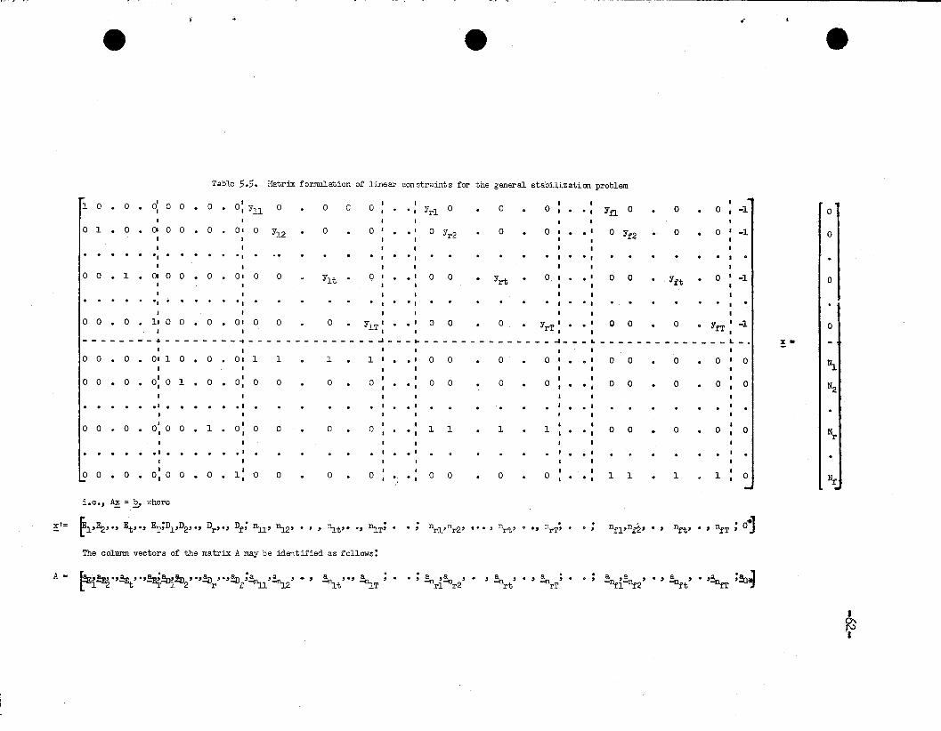
Table 5.5. I'latrix formulation of linear constraints for the general stabilizaticm problem
1 0' 0I 1 1 1 10 · 0 · I
0 · 0 · 0, Yll 0 · 0 C 0 , · ·, Yrl 0 · 0 · 0 , · • 1 Yfl. 0 · 0 · 0 1 -11 I 0, , I , , 10 1 · 0 · ()J 0 0 · 0 · O. 0 Y12 · 0 · 0 I · ·' 0 Yr 2 · 0 · 0 , · • 1 0 Yf2 · 0 · 0 1 -11 I 0
11
" · · · · · ·, · .. · . · · , · ·, · · · · · · 1 · • 1I 1 , I 1
0 0 1 01 0 0 · 0 · 01 0 0 · Ylt · 0 , · • 1 0 0 · Yrt · 0 1 · • 1 0 0 · . Yft · 0 I -11 I 0· · 1 1 I I I 11 1 1 1 1 1
'1 · · · · · ·, · · · . · · 1 · ·, · · · · · · I · ·,1 I 1 , 1 1
0 0 · 0 · 11 0 0 · 0 · 0' 0 0 · 0 · YlT : · · ' 0 0 · 0 · YrT : · • 1 0 0 · 0 · YfT 1 -1 I 0I , , , 1
--~--------~--------------~---~----- _________ ~ ___ L ____ __________ L __ !.-1 , , I I 1 ,
0 0 · 0 · 01 1 0 · 0 · 01 1 1 0 1 · 1 , · ·, 0 0 · 0 · 0 1 · o 1 0 0 · 0 · 0 1 0
I~1 , 1 , 1 1 1
0: 0 0' 1 , I 1 10 0 · 0 · 1 · 0 · I 0 0 · 0 · 0
I · • 10 0 · 0 · 0 1 · • 1
0 0 · 0 · 0 1 01 1 1
.1 · · · · · ·, · · · . · · , · ·, · · · · · · I · • I . . · . · . I
1 I I , 1 I
I0' I 1 I 1 1
0 0 · 0 0 0, 0 0 · 1 · 0 0 · 0 · 0 , · • 11 1 · 1 · 1 1 · • 1
0 0 · 0 · 0 1 01 I NrI, 1 , 1 1.1 · · · · · • I · · · 0 · · , · · ' 0 0 · · · · 1 0 • 1, , I , 1 1
I I' I I0
1 I1 1 1 1
~0 0 · 0 · 0, 0 0 · 0 · 0 0 · 0 · 0 I · · , 0 0 · 0 · , · • 1 · · 1 l N~. 1
i.e •• ~ = E" where
x '= fi.~.·. Et ••• ET;!1.·D2,·· Dr'" Df ; nu· ~2' • , • ~t" •• ~T; •. nrl,nr2 , ••• , nrt, o .J nrT~
.nfl·nf~· nft' • • nfT ; Gi· , · · , • •
The colunm vectors of the matrix A may be identified as follows:
A = r:'~"!g ,..~.:v'!D •••.:v ,••~ ;~ '~ , • • ~ "'!n, ; • ; a ,a , , a , o , a ; · . a a o , a , ••a ;~· . o ,-nri-Ilr2'1 -'I; 1 2 r f 1 2 t .LT -nr1-nr2 -nrt -nrT -nft -nfT
•0",~
..
-63-
be better to use the corresponding Dr. Hence, such a variable and its
corresponding column vector in the matrix .4 can be deleted_, We may
assume that for each r there exists at least one nrt with a corresponding
Prt '>o;otherwise, the resource should not have been considered.
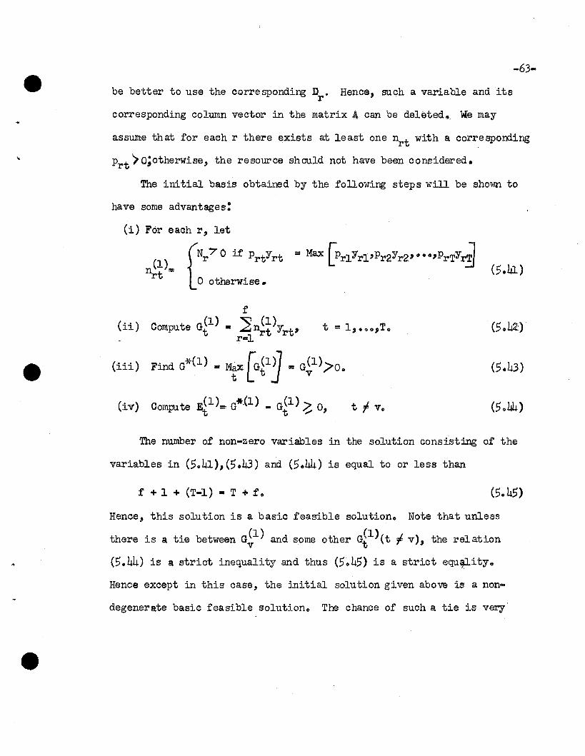
The initial basis obtained by the following steps will be shown to
have some advantages:
(iv) t r vo
The number of non-zero variables in the solution consisting of the
variables in (5.41),(5.43) and (5.44) is equal to or less than
f + 1 + (T-l) =T + f o
..
Hence, this solution is a basic feasible solutiono Note that unless
there is a tie between G~l) and some other Gi1)(t r v), the relation
(5.44) is a strict inequality and thus (5.45) is a strict equ~ityo
Hence except in this case, the initial solution given above is a non-
degenerate basic feasible solution. The chance of such a tie is very'
-64-
small and even if it oc~s, degeneracy can be avoided by changing
slightly the value of some Nr • To simplify the following development~
we will. assume that all basic solutions obtained are non-degenerate.
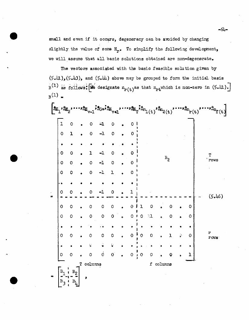
The vectors associated with the basic feasible solution given by
(5.41),(5.43), and (5.44) above may be grouped to form the initial basis
B(l) as fo±idW~: ~~ designate ~(t)as that ~twhich is non-zero in (5.L1)J
B(l) =
~ . .. ~!E '!E, •••'!E '~'!E ' ..•'!E ,!~ ~~ '···'!n '···~!n1 2 v-l v+l T .L(t) 4::(t) r(t) :t'(t
1 0 • 0 ~l 0 • 0 II
0 1 0 -1 0 0I
• • II
• • • • • • .. I• I
0 0 1 -1 0 0 I• • Te I B20 0 0 -1 0 0 I 'rows
• • I
0 0 0 -1 1 0I
• • I
I~. • • • • • • • I
I0 0 • 0 -1 0 .. 1 I= -- - - -- - - --- -- - -1 - - - - (5.46)
0 0 • 0 0 0 • 0,1 0 .. 0 .. 0
•0 0 • 0 0 0 .. 0 , 0 :'_1 • 0 .. 0~
I.. • .. • . .. • .. .. .. • .. .. .. •,0 0 0 0 0
,0 0 1 0
r0 • • .. ,~'\
rows.. •W
,.. .. .. .. ... .. • , .. .. .. • .. ..•0 0 .. 0 0 0 • 0 , 0 0 .. 0 .. 1,
T columns f columns
~l_:_B~,
= ,B3 : B4
-65...where Bl (T x: T) is a speciaJ. f onn of an elementary matrixo It is an
identity matrix except for the vth column which consists of ~ual
elements" -1;B2 (T x f)' is such. that the t th element in the r th column
~ ~rt if ~ti. in the baBis,
(0 otherwise;
B3(f x T) is a null matrix and B4(f x f) : If 0
B1 has the following properties:
(i) J Bl ): -1 ; (ii) Bil : Blo
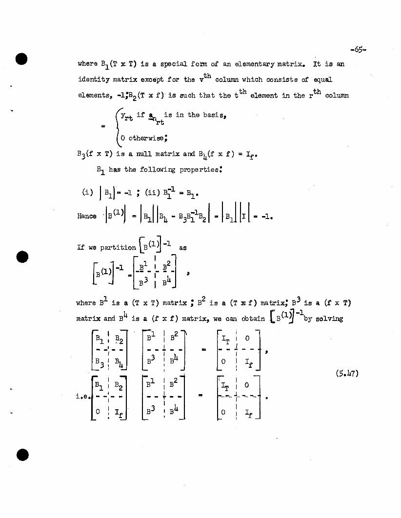
Hence !B(l>j a I~IIB4 ~ Bfli1B21-1BJ II I- -1.
where Bl is a (T x T) matrix; B2 is a (T :Jll: f) matrix; B3 is a (f x T)
matrix and B4 is a (f x f) matrix, we can obtain [B(lH -lby solving
I Bl I B2 IBl , ~2 I IT I 0
--I - - - - .!. - - • - - 1 - -( IB4
, ,B3
I B4 B3 I 0 I IfI I,
(5.47)I
Bl B2 {Bl I B2 Ir I 0
i.e. • t- = - J-- - - - -.. - ..-~- -- --I 1- 0
I B3I
B4 I0 • If I 0 I If• I
-66-
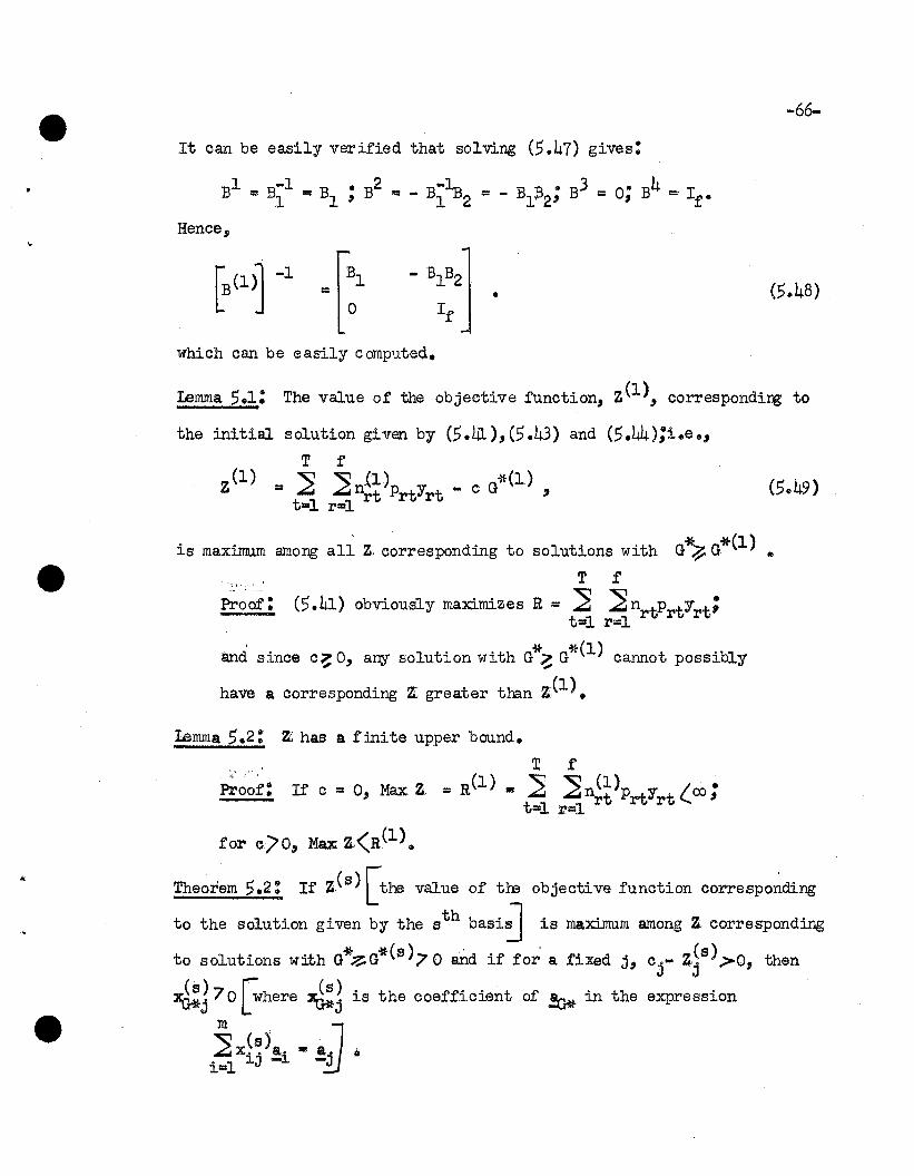
It can be easily verified that solving (5.47) gives:
Hence,
• (5.48)
which can be easily computed.
Lemma 5.1: The value of the objective function, Z(l), correspondirg to
the initial solution given by (5.41),(5.43) and (5.44);i.e.,
T fZ(l) == ] ]n{l)p y. _ c G*(l) ,
t==l ral rt rt rt
o ° 11 Z dO t 1 t' °th G*Z G*(l)J.s max:unum among a, correspon mg 0 so u J.ons WJ. ~. •
'-;.-
Proof:
T f
(5.41) obviously maximizes R = ] ]n tPtYt;t 1 1
r r r== r=
and since c~ 0, any solution with G*~ G~~(l) cannot possibly
have a corresponding z:: greater than Z:(l).
Lemma 5.2: Z:: has a fmite upper bound.
Proof:
for c/O, Max Z::(R(l) ..
Theorem 5.a: If Z(s) [the value of tre objective function corresponding
to the solution given by the sth basi~ is maximum among Z. corresponding
to solutions with G*~G*(S)70 and if for' a fixed j, cj - z.~s)>0, then
~J 70 [where ~5 is the coefficient of ~ in the expression
]x~~jai = a.;l.i=l J.J - ~
-67
Proof: If for a fixed j" c j - J:3S)/ 0" there exists by Theorem 4.7
and Lemma S 02 a f inite
.[x~S)~Q.... Minl ..~ '70,J .; .... \SJ
J. x .., J.J
(S.llO)
such that
exist llA-:l] 01 + [r:\st llj>4j~ 02 +•••+ [ ~s)_ llj";'~~ "m
+ Qjc. := z,(s) + Q. [C.- z,~s 51 ... z.(s+l),> z:(s) , (S.lAa-)J J J J J
."
where'in (S .. 410) and (Solll)
[x,(s)l t ... r2:,.(s) . ~s) xes~ is obtained by ._ ~ ~~ '000' ~ , .. o",_~ J
:~x(s) ",,~(s)f-lb ..L- 11 J -
S:ilnilarly.9
[x~s)l' .fx..(~~"ooO~X~~)'GOO"X(~~is obtained by-J J ~~J. J.J mJ]
x~s) • [B(s)l-l a. (>
-J j-J
Without any loss of generality, let
xeS) !!Jl a*(s) 7'0 and xes) "" xes)m mj G*j"
From (5.41.1) and (S.ll2)
(a+1) (s) QX(.S) G*(s) Q (s)~OJIhi "" ~ - j-tIlj" - j~j" ,
• 1'>__ G*(s+l) G*(s) _ Q; (s) '" 0J.,,-., ... jXG*j'~ 0
• I-
..
(s)Assume x"...... <. 0 ~U"C"J-/
We then have from (5",L13) that G*(S+1)~G*(8),
~(s+1)7~(s) 0
-68
(5.L14)
This contradicts the assumption in the theorem'that Z(s) is maximum
among all Z corresponding to solutions with G*~ G*(8); hence,.....
(5<)414) must be false; ioe,,~ ~~>o.
5~5 A Criterion for ~electing the Vectorto be Introduced into the Basis
Theorem 5<\>3: If Z(s) is maximum among all Z corresponding to solutions
With G~ G*(s)7 0, and if among the vectors with c.- Z~S)70, the vector
corresponding to ~ rCj-(:jS)l is introduced ~to :he (s+l)th basis,J [ xO*j J
then Z(s+l) is max:i.mu.m among all Z, corresponding to solutions with
G*? G*(8+l) ·h G*(8,+1)/ G*(8)E/ . , were .... 0
Proof: If for a fixed j,ll c j - Z,3 S );>O, then ~170 (by Theorem 5.2).
By TheDrem 407 and Lemma 50 2 there exists a finite
Qj & ~ rxf:~;> 0,1 Gj 1/
such'that Z(s+l) 00l Z;(s) + ~. rc .... Z:~8~ / Z;(S), (5 .. 51)J Ll
J J.J
and G*(13+l) !lli G*~s) .. Q.x~~~ <G*(8) co (5.52-)J ~J
-69-
5\1bstituting in (,.51) we obtain
Z;(s+l) =:a(S) + b-(:i1 ~i>(~? _ 0*(s+12 •
XU*j
In (5.54) tj~A '7 0 represent s the increase in Z; resulting
from raising the level of the j th variable enough to decrease G*
by one unit. Hence if among the vectors with c j - Z3s )/0" the
vector corresponding to
~ [~j~FJis introduced into the (S+l)th basis, the corresponding ~(S+l) is
maJl=imum in the interval G*(s+l)L (;.*<. G*(S)" where G*(s+l) is'
determined by ~bstituting in (,.,2.) the Qj
cor;responding to the
vector chosen by this criterion.' Moreover since by assumption in
the theorem" z:(s) is max:im:um in the interval G*~G*(Sl" we have
that z:(s+l)rz:(s) is maximum among all Z corresponding to solutions
with G*Z G*(s+l).
Theorem ,.4: Assume the following conditions are satisfied:
corresponding to feasible solutions with
T f
all R = ~ ~ l'lz.t1'rtYrt corresponding tot=l r=l
a) z:(s) is maximum among all Z
G*~G*(S»o•
b) Ri(S) is max:i.nIum among
..
feasible solutions with G*~ G*(s) 0; i.e., if G* is decreased" Hi
cannot be increas~d. Note that R(l) has this property.
-70-
c) Among the vectors with c. - Z;~s)70, the vector that correspondsJ J
to~ ["J~~~J is introduoed into the (S+l)th basis.
Then R(s+l) is max:inn.un among all R corresponding to solutions with
G*~G*(s+l)•
Proof: If condition (a) is satisfied, and if c. - Z;~s»o, thenJ J
x&~) .>0 by Theorem 5..2. Consider a fixed a. such that c.- Z~~S» 0,U*,J -J J J
where condition (a) is satisfied and let x~s)= G*(s) and
x(s~ = ~~). It
m,J -U*,J
c.- Z;(s)J j
== c.J
= c. -J
m-l~ (s) ,,(8)~ Xi' c. + cxG* ji=l J ~ ,
,"
=- A)s) + cxd:~)O ;
. (8) _ (s) ( (8»~.e., A. - c~.~. - c. - Z,. •
J " IJ'R'J J J
We first show that A~s)~O.J
(5055)
If
..
•
-71-
but this contradicts assumption ·~b); hence if conditions (a) and
(b) are satisfied, AYI)~ o.
[
0 z;(s)] [A(S) j~ j:a:i . · IIaX -.J~,. + 0 oorresponds to:
,j -~,j
(5.56)
~n E3·)/~;J ;. o.
Hence if condition (c), as well as conditions (a) and (b h are
satisfied, R(s+~) as given in (5.55) is maximum among all'R
corresponding to feasible solutions with G*£: G*(a+l). we also
have proved:
C.orollarz: Under conditions (a) and (b) in Theorem 5.4,A(s) .. exi~) _ fe _ z(s)l ~ 0
j .li*j tj jJ~ •
•
-72-
In the following development we will assume that:
(1) The iterative procedure is started with the initial basis B(1) and
the associated extreme point solution obtained by steps (i), (ii),
(iii) and (iv) in section S04•
(2) The vector to be introduced into the (s+l)th basis is that which
corresponds to Mi.'n [IJ. ~s) / ~~~J >. o.(s) J \fll-J"/
XOil-j 70
(3) The vector to be eliminated from the basis is determined by the
regular simplex rule (Case I of Theorem 4.7; since by Lemma S.2
Z', haa a finite upper bound, there is no possibility of encountering
Case II of Theorem 4.7).
(4.) The problem is non-degenerate.
Let .Min rlJ.~S) /xd:J] == ).(13)'
xd:J? 0 L'We need to prove the following lenuna.
Lenuna S.. 3: The sequence of ).(s) obtained in the success i ve changes of
basis is monotone non...decreasing;ioeo, A.(l)~ >..(a~ .... ~~(S)~).(S+l~....
Proof:
(a) we first prove that ).(2)~).(1).
(i) If >..(1) == 0 the proof is obvious, since ).(2)~ 0 by the
corollary to Theorem S.4.
(ii) Assume A.(l)~Oo For any c.- Z;~1) with ~~~)O, we canJ JU*J
write: or 1lJl) = ~~ rc - A~~~J. (S.S7)L ~j
(ii)
-73-
In the interval,
o ~ c ~ A(1)
no c.- z:~l) can be positive; hence, x(l) would be anJ J
optimal solution.
(iii) Assume that A(2)4 A(1). This implies that for any value
of c in the interval,
O~c~lo(2) , (5.59)
x(2) is an optimal solution. This is a contradiction,
since the interval (5.59) is contained in the interval
(5.58). Hence lo(2){. },(l), i.e., lo(2)~ lo(I).
(b) Vie next prove that lo(3)~lo(2)?lo(1). If lo(2) =t lo(l) == 0,
the proof is obvious (as above). Assume A(2).> O. Two cases
can arise:
(i) lo(2) "lo(l)~ O. In this case~(l) is an optimal
solution in the interval ~ c~ A(l)J , and ~(a) is
an optimal solution for
c = A(1) == A(2) , [Max Z(l) == Max z:(2) for t his value
of c7§
A(2) A(I)~ O. In this case 2:(1) is an optimal solution
for any value of c such that 0 ~ c~lo (1) .. (Note that if
>..(1) ... 0, 2:(1) is optimal only for c = 0.) Similarly,
2:(2) is an optimal solution for any value of c such
that A(l)~ co( A(2) ..- -
-74-
The assumption that A.(3)~ A. (2) implies that for
c = A.(.3~ 1.(2), '!:.(3) is an optimal solution. This contra
dicts either (i), (ii) or bothe Hence, 'A(3){ A.(2), and
in general 'A(3) ~ A. (2)~ A.(1).
(c) By an obvious extension of the se arguments, it is easy to see
that the lemma is true.
The results of the lemmas and theorems of Sections 5.4 and 5.5
suggest the following procedure ...
5,,6 A. Procedure for Findillg the Optimal Solutions (One or More)to the Gener al Production Stabilization Problem
f or Each Value of c in the Interval c ~ 0
(1) Find the initial basis B(1) and the asso ciated extreme point
solution, '!:.(1), by steps (i), (ii), (iii) and (iv) of Section 5.4.
(2)
(4)
(5)
If c = O~ this is an optimal solution.
Compute [B(lfl-1
as given in (5.48) ..
Obtain x~l) "" rB(l),-lQ. j = l!Juo,n.-J L::J -J'
Determine Min LA~1 }/x~G • 1.(1};
~j~O
If A(1) "" 0, :(1) is optimal only if c = 00 If 'A(1);> 0, '!:.(l) is
optimal for any value of c wch that 0 ~c ''A(1) •
Introduce the vector that corresponds to 'A(1) into the second basis
and eliminate a vector by the regular simplex rule (Case I,
Theorem 4,,7) ..
-75-(6) Determine l(2). By Lemma $.3, A(2)~l(1). If l(2):1 l(l),
!(2) or ~(l) are alternative optimal solutions, for c = A(2):I l(l).
If A(2) >A(1), ~(2) is an optimal solution for c in the interval
A(l~ C~A(2).
(7) If the above criterion is successively used, we can, for each basis,
determine a closed sub-interval of c such that the extreme point
solution associated with the given basis is an optimal solution for
any value of c in that alb-interval. It is possible that the
lower and upper limits for a sub-interval obtained at a given basis
are equal; i.e., that there is only one value of c such that the
corresponding solution is opt:ilnalo In this case the solution
corresponding to this particular basis and that obtained in the
preceding basis are alternative optimal solutions for this value of
c.
(8). As long as the value of Z corresponding to any particular value of
c in a sub-interval derived by following this procedure is greater
than zero, the pro ces s can be co nt inued I)
(9) We cannot remain indefinitely at a value of l (a)= Co (say). For
suppose that we want to solve the problem for some c v~co. It is
clear that we can write any cj- Z.3 s ) that might be positive in the
sth basis as:
x~~ t' -$iJ ·Hence the steps that would be followed to solve the problem for
C :I c' must be exactly tb3 same as those followed until we reach
•
""76
the value X(s)=. cO* The asswmption of non-degeneracy guarantees
that we must be able to solve the problem for c := Ci. Hence we
cannot obtain a value A(s) = Co such that the lower and. upper
limits obtained in each succeeding iteration remain indef:initely
equal to cO. After we leave a basis, we cannot return to it or
to any basis corresponding to a lower value of c.
~: The remarks made in step (9) are suggested by some remarks
made by Gass G-958) in a similar si tua tiono
(10) The process will terminate by finding a finite value
T
C ~ ~ Max(PrtJ such that if C4C, the optimal allocation plantal r '
has a corresponding value of Z = 00
One can summarize these resu.lts as follows:
(a) If c = 0, !(l) is an optimal solution"
If c = a = A(l) = 0 •• =A(h)~A(h+l)9 ~(l)$~(2)$ooOg~(h) are
all optimal solutions.
(b) If O~C(A(l), !(l) is an optimal solution.
(e) If A(t-l) (. C <A(t),' !(t) is an optimal solution.
(d) If·· O(c. ,(h) .,(h+l) _ . ,(t)/,(t+1) (u.) (h+l) (t+l)= A ... A - ...... A ~ A $~'! $" •• ,.!
are all optimal solutions •
6.0 Surrnnary and Limitations and Extensionsof the Studied MOdel
6 01 Sunnnary
This dissertation is concerned with the decision problem faced by a
firm which produces a non-storable connnodity and has to spend large
amounts of capital on a specialized factor that could be idled part of
the t:ime by fluctuation in production., In partimlar, it is assumed that
the firm uses f resources, Nr units of the r th resource being available
for production., These resources are to be allocated to one or more of
th thT different time periods, nrt units of the r resource to the t
period. Each of these I1:rt units can produce Yrt units of output at a
price less direct variable costs of Prt each;ioeo~ the total returns
f
are It = ~r=l
T
~nrtYrtPrt·tal
The decision problem is to determine the
which maximizes . ~f ~
z: := R - c Max ] I1:rtYrtt r=l
subject to the restriction ~I):.t4fNr and !1:rt~O., The cost of thet
specialized factor for being available :1n any of the T time periods is
approxLmated by a constant nmltiple of the maxinmm production in any
one time period. A detailed discussion of this matter is presented in
Section 2.30
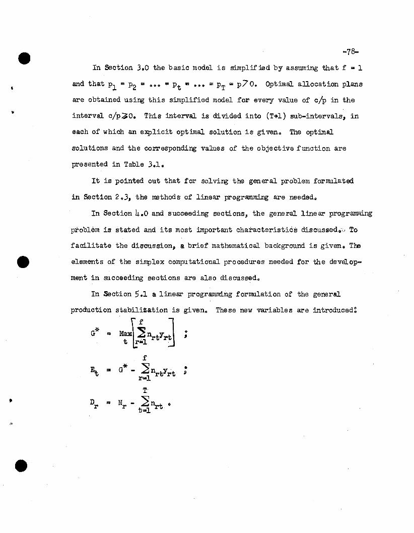
•,
,
•
-78-
In Section 3.0 the basic model is simplified by assuming that f =: 1
and that Pl = P2 == 00. =Pt == .... == PT =p7 O. Optimal allocation plans
are obtained using this simplified model for every value of c/p in the
interVal c/p~O. This interval is divided into (T+l) sub-intervals, in
each of which an explicit optimal solution is given. The optimal
solutions and the corresponding values of the objective function are
presented in Table 3.1.
It is pointed out that for solving the general problem forIlUllated
in Section 2.3, the methods of linear programming are neededo
In Section 4.0 and succeeding sections, the general linear programnlng
problem is stated and its most important characteristics discuslBedo:' To
facilitate the discussion, a brief mathematical background is given. Th9
elements of the simplex computational procedures needed for the deveU.op-
ment in succeeding sections are also discussed.
In Section 5.1 a linear programming formulation of the general
production stabiliZation is given. These new variables are introduced~
G* = MaEI~"rtyJt '~=l ~
T
-~nnotal
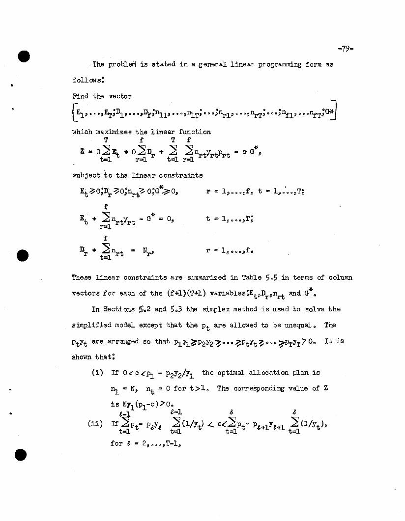
-79-
The probleni is stated in a general linear programming form as
follows:
which maximizes the linear functionT £ T f
z: = O~Et + O~D~ + ~ ~nrtYrtPrttal r=l t=l r=l
subject to the linear constraints
'"
£
Et· + ~n t Y t. - G* = 0,1
r rr=
T
n~ + t~nrt = Nr ,
These linear constraints are mmmarized in Table $,,$ in terms of column
vectors for each of the (f+l){T+l) variables~EVDr9~tand G*.-
In sections $,,2 and $,,3 the simplex method is used to solve the
simplified model except that the Pt are allowed to be unequal" The
PtYt are arranged so that PlYl~P2Y2 ~"u ~PtYt ~ "0" ~PrYT 7 00 It is
shown that:
(1) If 0 < c <'PJ. - P2Y2/Yl the optimal allocation plan is
~ "" N, nt "" 0 for t >1" The corresponding value of Z
is NYl (Pl-c) .> 0",.e-l .e=l .e .e
(ii) If ]Pt- P.eY.e. ~ (l!Yt) <.. c<'~Pt= P.e+lY.e+l ~ (l!yt ),t=l t=l t=l t=l
for.e = 2,o •• ,T-l~
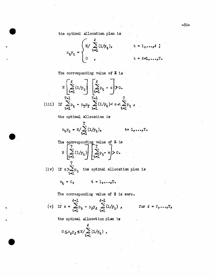
the optimal allocation plan is
~
N/ ~ (l/Yt)'tal
,
The corresponding value of Z: is
t ... 1, •••,~ ;
t i= ~+l, ...,T.
-80-
Nr] (l/Yt1 r]Pt - ;)0.~=l ,:J ~=l :J
T-l T-l T
(iii) If' ~Pt - PTYT ] (l/Yt)<: eL.]pt 'tal tal t;:l
the optimal allocation is
T.
l1.tYt =- N/] (l/Yt),tal
t= 1, ... ,T.
The corresponding value ofZis
N f] (In) f]pt- J o.b=l J Lt=l J
T
(iv) If' c>~Pt the opt:i1nal allOCation plan istal
l1.t = 0, t ... 1, ... ,T.
The corresponding value of Z i~ ~ero.
~-l ~-l
(v) If c = ~Pt - PiY~ ~ (l/Yt) ,tal t;:l
the optimal allocation plan is
.eO$n~Y~~N/~ (l/Yt) ,
tal
for ~ = 2, o ••,T,
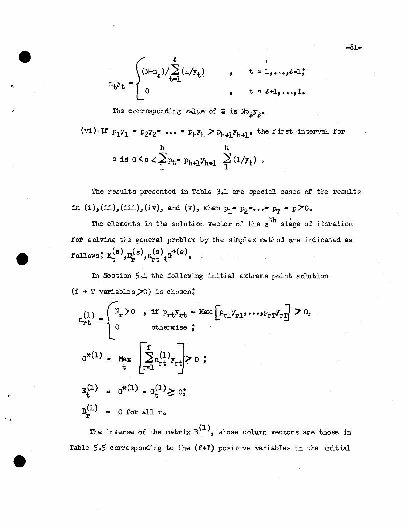
.t(N-n.t)/] (l/Yt)
t=l
o
, t = 1, ... ,.t-l;
t - .t+l, •••, T.
-81-
~ 0,
The corresponding value of Z is NP.tY.t.
(v.O::J:f PlYl = P2Y2= ... • PhYh;> Ph+lYh+l' the first interval for
h h
c is 0 <c <~Pt- Ph+lYh.l ] (l/Yt) •1 1
The results presented in Table 3.1 are special oases of the results
in (i),(ii),(iii),(iv), and (v), when PI= P2-•••- PT =p;>O.
The elements in the solution veotor of the sth st~ge of iteration
for salving the general problem by the simplex method are irrlicated as
follows " E(.S) "",(s) n(S).G*(S)o . t ,~ '-~t I •
In seotion 504 the following initial extreme point s olution
(f .. T variable s /0) is chosen:
~) • 0r:>O • i:t PrtYrt • Mal< [PrlYrl'....Pr~r~~o otherwise ;
"
.~
E(l)t
n:(l)r I: 0 for all ro
The inverse of the matrix B(l), whose oolumn veotors are those in
Table 505 corresponding to the (f+T) positive variables in the initial
•
-82-
solution, can be easily computed. The initial solution has the following
properties: T f
(1) R(l) = ] ] n~~)PrtYrt is a maximum R.t=l r=l
(2) Z(l) = R(l) - c G*(l) is maximum among all Z, corresponding to
solutions with G*~G*(l).
The linear programming procedure starts with an initial solution,
such as that, given above; determines if one of the omitted variables
can profitably be added; and, if one can profitably be added, deter
mines which of the original set should be removed. Z(1) would be
changed by an amount c j- zjl); for each unit of'the j:tli variable if intro
duced into the system, where c j represents the added returns due to
the jth variable and Z~l) the change in Z(l) due to changes in the otherJ
variables needed to satisfy the constraints. If at least one c.- ~~l)J J
is positive, that variable is added for which cj - z31»0 and
c.- Z;~l)J (i~ is a maximum, where ~~ >0 is def:ined in Theorem 5.2. .4XO*j
criterion is given in Case I, Theorem 4.7 for determining which of the
original f + T variables associated with B(l) is replaced by the jth
one. The suggested criterion for determining which variable should be
added:m~imizes the increase :in Z(l) for a unit decrease in G*.(l).
By successively following this procedure, starting with the vari
ables associated with B(l), every solution obtained will have the
following properties:
(1) R(s) is maximum among all R corresponding to solutions with
G*~ G*.(s) ..
-8.3-
(2) Z:(s) is maxinrum among all solutions with G*~ G*(s).
A procedure is suggested for finding the optimal solutions to the general
production stabilization problem for each value of c in the interval"
c~O" The details of this procedure are presented in Section 5.6.
6 0 2 Limitations and Extensions of the Studied Model
It must be realiZed that no mathematical model simple enough to be
manageable can provide complete solutions for the complicated decision
problems that confront a firm in the real world. However, as Dorfman
L195~ states:
II'Simplified models serve a real purpose in enablingus to deal intellectually with at least some ,forcesat work in the real economic world. They perform,partlY9 the function or an experiment under controlled laboratory conditions .. '"
Model building is a multi-stage .process. .A useful beginning
tOWjl.rds obtaining approximate solutions for the complicated decision
problems of the real world may be made by formulating a simplified model
which omits some factors that are present in the true situation, arrl;
solving the problems presented by the simplified model. The model may
then be enlarged to a more comprehensive model by including some of the
factors that have been omitted in the initial formulation. Solutions
are then sought for the problems presented by the enlarged model 0 The
solutions already obtained will usually help in attempting to solve the
more complex problems of the enlarged model 0
-84-
The model studied in this thesis could be extended in many directions:
(1) It might be desirable to relax the assumptions that the firm can sell
any quantity it can produce, in any of the given t:ime periods" and
without affecting the market price at that time period. TIlis may be
achieved by one of the following:
(a) In solving the linear programming problem formulated in
Section 5.1, additional constraints may be imposed on the
allocation variables. For example:~.
] nrtYrt ~ ~t' t = 1, ..., T,r=l
where Qt is an upper limit on the quantity that the firm
can sell in time period t.
(b) Instead of aSS1.Uning that the price at any given time period
does not depend on the firm's production in that time
period, we can assume a knowledge of the demand function
that relates the firm's production in any given time period
to the price it receives for the commodity at that time
period. If these demand functions are assumed to be linear,
the problem can be formulated as a problem of quadratic
programming.
(2 ) We have assumed that the only costs that may make a fluctuating
production schedule an unefficient one are those investment costs
incurred by the firm in order to have enough units of a specialiZed
factor to accommodate the maximum production by the firm in any of
T time periods. This assumption was made to emphasize the effects
•
-85-
of such costs on the firm's allocation plan. Other costs associated
with a fluctuating production schedule (e.g., costs of hiring and
releasing personnel) may also be included in the model if they are
considered important. For example, we can write
f f
~nrtYrt - ~nr t-1Yr t-l = qt - st' t = 1, ... ,T,r=l r=l'.9
where qt~ 0 represents an increase in production, and St~ 0
represents a decrease in production;i.e., if qt:( O,St => °and vice
versa, we can include qt'St (t=l, ...,T) among the decision variables
and assign to them appropriate costs in the objective function.
The restrictions on the decision variables would thus be augmented
by the set of equations:f f
r~nrtYrt - r~nr,t-1Yr.9t-l - qt + St == 0, t => 1, ...,T,
0) We have assumed that the amount of the r th resource (I' => 1, 0 ..,f)
that can be allocated by tb3 firm to produce in any of tb3 T time
periods is limited by a constant, Nr , which does not depend on the
allocation plan chosen by the firm. For any unit of this resource,
we are concerned with a single allocation to any of the T time
periods 0 In other words, we are not concerned with how that unit
will be re-allocated once a production process terminates. How-
ever, if the time interval over which the allocation plan is
required is long enough so as to permit successive production
processes on the same unit of any of these resources, the quantity
available from any resource for starting new production processes
•
-86-
at a given time period will depend on how the units of that resource
were allocated at some previous time periods. The model studied in
this thesis could be extended so as to account for such dynamic
features in the allocation plan chosen by the fir.m.
(4) The model discussed in this dissertation is deterministic. By
assuming that the relevant market and technologipal conditions are
known with certainty, we have evaded some of the most critical
problems that confront the firm. Fu.rther research to introduce
random errors into the studied model is needed. Random errors
might be introduced in one or more of the following:
a) The prices received by the firm for its products.
b) The yields Yrt; r =l, •••,f, t =1, ••• ,T.
c) The time needed for a production process to be completed.
If random errors are introduced into the model, a problem of a
different nature arises. The subjective attitude of the entre
preneur towards risk has to be taken into consideration.
•
-87-
LIST OF REFERENCES
Allen, R. G. Do 19560 Mathematical Economics. The MacMillan Co.,New York ..
Charnes" AO $ Cooper:.> W. W" and Farr$ Do 195Jo Linear programming andprofit preference scheduling for a manufacturing firm .. Journal ofOperations Research Society of America, Vol. 1.
Charnes" Ao , Cooper, W. W. and Henderson, A.. 1953. Introduction toLinear Programming" John Wiley and Sons, Inc., New York.
Dantzig.ll G. Bo 1951.. Maximization of a linear function of variablessubject to linear inequalities. Chapter XXI in Activity Analysisof Production and .Allocati ono Edited by T. n: Koopmans. CowlesCommission Monograph 13$1 John Wiley and Sons, InG. New York.
Dantzig:.> G. B"$! Orden$) A" and Wolfe.9 P~ 1954" Generalized SimplexMethod for Minimizing a Linear Form Under Linear InequalityRestraints.. RAND Report RM-1264" The RAND Corporation,Santa Monica,\) California..
Dorfman$) Ro
Firm.1951.. Application of Linear Programming to Theory of the
University of California Press, Berkeley, California.
Gass, S" 10 1958.. Linear Programming)! Methods and Applications.McGraw;=Hill,Book COo$l Inc.. New Yorko
Hoffman$) A. Jo 1955" How to solve a linear programming problem.ppo 397-424 in Directorate of Management Analysis: Proceedingsof the SeconaSymposium in Linear Programming.. Edited byH.. Antosiewicz" DeS/Comptroller)! Headquarters, UoS .. Air Force,Washington$) D. Co
Karlin, So 1959.. Mathematical Methods and Theory in Games,Programming and Economics 0 VoL 1.9 Addison-Wesley PublishingCo".9 Inc.. Reading,\) Massachusetts"
Riley, V" and Gass,\l So I.. 19580 Bibliography on Linear Programmingand Related Techniques" Johns Hopkins Press, Baltimore, Maryland.
Simmonds, No W'" 1959.. Bananas.. Longmans Green and Coo, Ltd., London,England..
INSTITUTE OF STATISTICS
NORTH CAROLINA STATE COLLEGE
(Mimeo Series available for distribution)
258. Hoeffding,Wassily. On sequences of sums of independent random vectors.
259. Webster, J. T., A. H. E. Grandage, R. J. Hader, R. L. Anderson. A decision procedure for the inclusion of an indepen-dent variate in a linear estimator. June, 1960.
260. Chakravarti, I. M. On some methods of construction of partially balanced arrays. July, 1960.
261. Roy, S. N. and R. Gnanadesikan. On certain altemative hypotheses on dispersion matrices. August, 1960.
262. Murthy, V. K. On the distribution of averages over the val'ious lags of certain statistics related to the serial correlationcoefficients. August,}960.
263. Anderson, R. L. Some needed developments in multivariate analysis. August, 1960.
264. Chapman, D. G., W. S. Overton and A. L. Finkner. Methods of estimating dove kill. October, 1959.
265. Eicker, FriedheIm. Consistency of parameter-estimates in a linear time-series model. October, 1960.
266. Eicker, FriedheIm. A necessary and sufficient condition for consistency of the LS estimates in linear regression. October,1960.
267. Smith, W. L. On some general renewal theorems for nonidentically distributed variables. October, 1960.
268. Duncan, D. B. Bayes rules for a common multiple comparisons problem and related Student-t problems. November,1960.
269. Bose, R. C. Theorems in the additive theory of numbers. November, 1960.
270. Cooper, Dale and D. D. Mason. Available soil moisture as a stochastic process. December, 1960.
271. Eicker, FriedheIm. Central limit theorem and consistency in linear regression. December, 1960.
272. Rigney, Jackson A. The cooperative organization in wildlife statistics. Presented at the 14th Annual Meeting, SoutheasternAssociation of Game and Fish Commissioners, Biloxi, Mississippi, October 23-26, 1960. Published in Mimeo Series, January, 1961.
273. Schutzenberger, M. T. On the definition of a certain class of automata. January, 1961.
274. Roy, S. N. and J. N. Shrizastaza. Inference on treatment effects and design of experiments in relation to such inferences.January, 1961.
275. Ray-Chaudhuri, D. K. An algorithm for a minimum cover of an abstract complex. February, 1961.
276. Lehman, E. H., Jr. and R. L. Anderson. Estimation of the scale parameter in the Weibull distribution using samples cen·sored by time and by number of failures. March, 1961.
277. Hotelling, Harold. The behavior of some standard statistical tests under non-standard conditions. February, 1961.
278. Foata, Dominique. On the construction of Bose-Chaudhuri matrices with help of Abelian group characters. February,1961.
279. Eicker, Friedheim. Central limit theorem for sums over sets of random variables. February, 1961.
280. Bland, R. P. A minimum average risk solution for the problem of choosing the largest mean. March, 1961.
281. Williams, J. S., S. N. Roy and C. C. Cockerham. An evaluation of the worth of some selected indices. May, 1961.
282. Roy, S. N. and R. Gnanadesikan. Equality of two dispersion matrices against altematives of intermediate specificity.April, 1961.
283. Schutzenberger, M. T. On the recurrence of patterns. April, 1961.
284. Bose, R. C. and I. M. Chakravarti. A coding problem arising in the transmission of numerical data. April, 1961.
285. Patel, M. S. Investigations on factorial designs. May, 1961.
286. Bishir, J. W. Two problems in the theory of stochastic branching processes. May, 1961.
287. Konsler, T. R. A quantitative analysis of the growth and regrowth of a forage crop. May, 1961.
288. Zaki, R. M. and R. L. Anderson. Applications of linear programming techniques to some problems of production planning over time. May, 1961.


