40
Applications of Neural Networks in Time-Series Analysis Adam Maus Computer Science Department Mentor: Doctor Sprott Physics Department
| Date post: | 01-Jan-2016 |
| Category: |
Documents |
| Upload: | armand-fowler |
| View: | 41 times |
| Download: | 1 times |

Applications of Neural Networks in Time-Series Analysis
Adam MausComputer Science Department
Mentor: Doctor Sprott Physics Department

Outline
• Discrete Time Series • Embedding Problem• Methods Traditionally Used• Lag Space for a System• Overview of Artificial Neural Networks
– Calculation of time lag sensitivities
– Comparison of model to known systems
• Comparison to other methods• Results and Discussions

Discrete Time Series
• Scalar chaotic time series– i.e. average daily temperatures
• Data given discrete intervals– i.e. seconds, days, etc.
• We assume a combination of past values in the time series predict the future
[45, 34, 23, 56, 34, 25, …]
Discrete Time Series (Wikimedia)

Time Lags
• Each discrete interval refers to a dimension or time lag
542 kkkk xxxx[45, 34, 23, 56, 34, 25, …]
Current Value
1st Time Lag
2nd Time Lag Current Value
2nd Time Lag ….

Outline
• Discrete Time Series • Embedding Problem• Methods Traditionally Used• Lag Space for a System• Overview of Artificial Neural Networks
– Calculation of time lag sensitivities
– Comparison of model to known systems
• Comparison to other methods• Results and Discussions

Embedding Problem
• The embedding dimension is related to the minimum number of variables required to construct the data
Or
• Exactly how many time lags are required to reconstruct the system without any information being lost but without adding unnecessary information
– i.e. a ball seen in 2d, 3d, and 3d + Time
Problem: How do we choose the optimal embedding dimension that the model can use to unfold the data?
-1.5
-1
-0.5
0
0.5
1
1.5
-1.5 -1 -0.5 0 0.5 1 1.5
Xk-1
Xk
Xk

Outline
• Discrete Time Series • Embedding Problem• Methods Traditionally Used• Lag Space for a System• Overview of Artificial Neural Networks
– Calculation of time lag sensitivities
– Comparison of model to known systems
• Comparison to other methods• Results and Discussions

ARMA Models
• Autoregressive Moving Average Models– Fits a polynomial to the data based on linear combinations of past
values
– Produces a linear function
– Can create very complicated dynamics but has difficulty with nonlinear systems
q
iiki
d
iikitk xßx
11

Autocorrelation Function
• Finds correlations within data
• Much like the ARMA model, shows weak periodicity within nonlinear time series.
• No sense of the underlyingdynamical system
Logistic Map
11 14 kkk xxx
The Nature of Mathematical Modeling (1999)

Correlation Dimension
• Introduced in 1983 by Grassbergerand Procaccia to find the fractal dimension of a chaotic system
• One can determine the embedding dimension by calculating the correlation dimension in increasing dimensions until it ceases to change
• Good for large datasets with little noise
Measuring the Strangeness of Strange Attractors (1983)
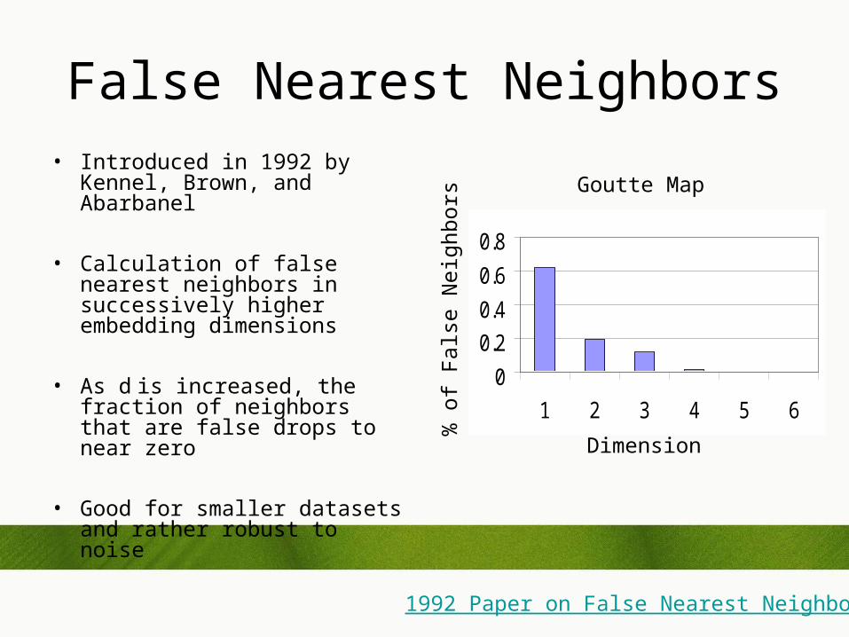
False Nearest Neighbors• Introduced in 1992 by Kennel,
Brown, and Abarbanel
• Calculation of false nearest neighbors in successively higher embedding dimensions
• As d is increased, the fraction of neighbors that are false drops to near zero
• Good for smaller datasets and rather robust to noise
1992 Paper on False Nearest Neighbors
% o
f F
alse
Nei
ghbo
rsDimension
Goutte Map
0
0.2
0.4
0.6
0.8
1 2 3 4 5 6

Outline
• Discrete Time Series
• Embedding Problem
• Methods Traditionally Used
• Lag Space for a System
• Overview of Artificial Neural Networks– Calculation of time lag sensitivities– Comparison of model to known systems
• Comparison to other methods
• Results and Discussions
542 kkkk xxxx
54321 00 kkkkkk xxxxxx

Lag Space• Not necessarily the same dimensions
as embedding space
• Goutte Map dynamics depend only on the second and fourth time lag
422 3.04.11 kkk xxx
Lag Space Estimation In Time Series Modelling (1997)
Goutte Map
Problem: How can we measure both the embedding dimension and lag space?

Outline
• Discrete Time Series • Embedding Problem• Methods Traditionally Used• Lag Space for a System• Overview of Artificial Neural Networks
– Calculation of time lag sensitivities
– Comparison of model to known systems
• Comparison to other methods• Results and Discussions

Artificial Neural Networks
• Mathematical Models of Biological Neurons
• Used in Classification Problems
– Handwriting Analysis
• Function Approximation
– Forecasting Time Series
– Studying Properties of Systems
m
jjkjkk xaby
1

Function Approximation
• Known as Universal Approximators
• The architecture of the neural network uses time-delayed data
Structure of a Single-Layer Feed forward Neural Network
x = [45, 34, 23, 56, 34, 25, …]
d
jjkiji
n
iik xaabx
10
1
tanhˆ
Xk-d
n
1
Multilayer Feedforward Networks are Universal Approximators (1989)

Function Approximation
• Next Step Prediction– Takes d previous points and predicts the next step
d
jjkiji
n
iik xaabx
10
1
tanhˆ

Training
1. Initialize a matrix and b vector
2. Compare predictions to actual values
3. Change parameters accordingly
4. Repeat millions of times
c
xxc
kkk
1
2ˆMean Square Error
c = length of time series
Fitting the model to data (Wikimedia)
kxkx
kx
1kx

Convergence
• The global optimum is found at thelowest mean square error– Connection strengths can be any
real number
– Like finding the lowest point in a mountain range
• Numerous low points so we must devise ways to avoid these local optimum

Outline
• Discrete Time Series • Embedding Problem• Methods Traditionally Used• Lag Space for a System• Overview of Artificial Neural Networks
– Calculation of time lag sensitivities
– Comparison of model to known systems
• Comparison to other methods• Results and Discussions

Time Lag Sensitivities
• We can train a neural network on data and study the model• Find how much the output of the neural network varies when
perturbing each time lag• “Important” lags will have higher sensitivity to changes in values
542 kkkk xxxx
1 2 3 4 5 6 7
Lags
Sen
siti
viti
es

Time Lag Sensitivities
• We estimate the sensitivity of each time lag in the neural network:
n
i
d
mmkimiiij
jk
k xaabax
x
1 10
2sechˆ
c
jk jk
k
x
x
jcjS
1
ˆ1ˆ
1 2 3 4 5 6 7
LagsS
ensi
tivi
ties

Expected Sensitivities
• For known systems we can estimate what the sensitivities should be
• After training neural networks on data from different maps the difference between actual and expected sensitivities is <1%
c
jk jk
k
x
x
jcjS
1
ˆ1
3.0
8.2
3.04.11
2
11
221
k
k
kk
k
kkk
x
x
xx
x
xxx
Outline
• Discrete Time Series • Embedding Problem• Methods Traditionally Used• Lag Space for a System• Overview of Artificial Neural Networks
– Calculation of time lag sensitivities
– Comparison of model to known systems
• Comparison to other methods• Results and Discussions
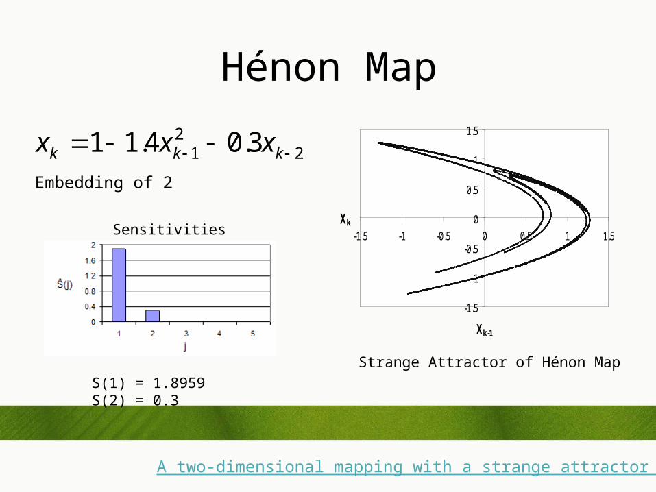
Hénon Map
221 3.04.11 kkk xxx
Strange Attractor of Hénon Map
A two-dimensional mapping with a strange attractor (1976)
-1.5
-1
-0.5
0
0.5
1
1.5
-1.5 -1 -0.5 0 0.5 1 1.5
Xk-1
Xk
Embedding of 2
Sensitivities
S(1) = 1.8959 S(2) = 0.3

Delayed Hénon Map
Strange Attractor of Delayed Hénon Map
High-dimensional Dynamics in the Delayed Hénon Map (2006)
dkkk xxx 1.06.11 21
Embedding of d
Sensitivities
S(1) = 1.9018 S(4) = .1

Preface Map “The Volatile Wife”
-1
-0.5
0
0.5
1
1.5
2
-1 -0.5 0 0.5 1 1.5 2
Xk-1
Xk
32121 6.09.02.0 kkkkk xxxxx
Embedding of 3
Strange Attractor of Preface Map
0
0.3
0.6
0.9
1.2
1 2 3 4 5
j
Ŝ(j) (a)
Sensitivities
S(1) = 1.1502 S(2) = 0.9 S(3) = 0.6
Chaos and Time-Series Analysis (2003)
Images of a Complex World: The Art and Poetry of Chaos (2005)

Goutte Map
422 3.04.11 kkk xxx
(d) Goutte Map
-1.5
-1
-0.5
0
0.5
1
1.5
-1.5 -1 -0.5 0 0.5 1 1.5
Xk-1
Xk
Strange Attractor of Goutte Map
Embedding of 4
0
0.4
0.8
1.2
1.6
2
1 2 3 4 5
j
Ŝ(j) (a)
Sensitivities
Lag Space Estimation In Time Series Modelling (1997)
S(2) = 1.8959 S(4) = 0.3

Outline
• Discrete Time Series • Embedding Problem• Methods Traditionally Used• Lag Space for a System• Overview of Artificial Neural Networks
– Calculation of time lag sensitivities
– Comparison of model to known systems
• Comparison to other methods• Results and Discussions

Results from Other Methods
Hénon Map Neural Network
False NearestNeighbors
CorrelationDimension
221 3.04.11 kkk xxx
Optimal Embedding of 2

Results from Other MethodsDelayed Hénon Map Neural
Network
False NearestNeighbors
CorrelationDimension
421 1.06.11 kkk xxx
Optimal Embedding of 4

Results from Other MethodsPreface Map Neural
Network
False NearestNeighbors
CorrelationDimension
32121 6.09.02.0 kkkkk xxxxx
Optimal Embedding of 3

Results from Other MethodsGoutte Map Neural
Network
False NearestNeighbors
CorrelationDimension
422 3.04.11 kkk xxx
Optimal Embedding of 4

Comparison using Data Set Size
• Varied the length of the Hénon map time series by powers of 2
• Compared methods to actual values using normalized RMS error E
d
j
d
j
jS
jSjS
E
1
2
1
2
)(
)()(ˆ
32 2048256
%
70
0
Where is predicted value for a test data set size
is actual value for an ideal data set size
j is one dimension of d that we are studying
S
S

Comparison using Noisy Data Sets
• Vary the noise in the system by adding Gaussian White Noise to a fixed length time series from the Hénon Map
• Compared methods to actual values using normalized RMS error
• Used noiseless case values for comparison of methods
High Noise Low Noise
%
0
100
180

Outline
• Discrete Time Series • Embedding Problem• Methods Traditionally Used• Lag Space for a System• Overview of Artificial Neural Networks
– Calculation of time lag sensitivities
– Comparison of model to known systems
• Comparison to other methods• Results and Discussions

Temperature in Madison
0
0.05
0.1
0.15
0.2
0.25
0.3
0.35
1 2 3 4 5 6 7 8 9 10 11 12 13 14 15 16 17 18 19 20
Dimensions
Se
ns
itiv
itie
s
4 neurons
16 neurons

Precipitation in Madison
0
0.02
0.04
0.06
0.08
0.1
0.12
0.14
0.16
1 2 3 4 5 6 7 8 9 10 11 12 13 14 15 16 17 18 19 20
Dimensions
Se
ns
itiv
itie
s
4 neurons
16 neurons

Summary
• Neural networks are models that can be used to predict the embedding dimension
• They can handle small datasets and accurately predict sensitivities for a given system
• They prove to be more robust to noise than other methods used
• They can be used to determine the lag space where methods cannot
-1.5
-1
-0.5
0
0.5
1
1.5
-1.5 -1 -0.5 0 0.5 1 1.5
Xk-1
Xk

Acknowledgments
• Doctor Sprott for guiding this project
• Doctor Young and Ed Hopkins at the State Climatology Office for the weather data and insightful discussions


