110

AFIT/GA/ENY/95D-02
Applications of Nonlinear Control Using
the State-Dependent Riccati Equation
THESIS
David K. ParrishCaptain, USAF
AFIT/GA/ENY/95D-02
Approved for public release; distribution unlimited
The views expressed in this thesis are those of the author and do not re ect the o�cial policy or
position of the Department of Defense or the U. S. Government.

AFIT/GA/ENY/95D-02
Applications of Nonlinear Control Using
the State-Dependent Riccati Equation
THESIS
Presented to the Faculty of the School of Engineering
of the Air Force Institute of Technology
Air University
In Partial Ful�llment of the
Requirements for the Degree of
Master of Science
David K. Parrish, B.S.E., Aerospace Engineering
Captain, USAF
December, 1995
Approved for public release; distribution unlimited
Acknowledgements
I would like to thank my reading committee, Dr. Can�eld and Dr. Spenny, for their comments
and suggestions, which have truly improved the quality of this thesis. I am also grateful to Dr.
Hall and Dr. Wiesel for their assistance, especially since I know they were both busy with thesis
students of their own. Most importantly I would like to express my thanks to my advisor Dr.
Ridgely for his support and guidance. He has taught me a great deal about modern control and
has motivated me to continue my education in this �eld.
I think I would be amiss to fail to acknowledge all the help my fellow students have also pro-
vided, from help with LaTEX to a multitude of other computer and control theory related questions.
I have certainly enjoyed the friends I have made here at AFIT.
My last thanks is to my family. Although they are far away, they provide the love and support
I need in the tasks that I undertake.
David K. Parrish
ii
Table of Contents
Page
Acknowledgements : : : : : : : : : : : : : : : : : : : : : : : : : : : : : : : : : : : : : : : ii
List of Figures : : : : : : : : : : : : : : : : : : : : : : : : : : : : : : : : : : : : : : : : : vii
List of Tables : : : : : : : : : : : : : : : : : : : : : : : : : : : : : : : : : : : : : : : : : : x
Abstract : : : : : : : : : : : : : : : : : : : : : : : : : : : : : : : : : : : : : : : : : : : : : xi
I. Introduction : : : : : : : : : : : : : : : : : : : : : : : : : : : : : : : : : : : : : : : 1-1
1.1 Overview : : : : : : : : : : : : : : : : : : : : : : : : : : : : : : : : : : 1-1
1.2 Objectives : : : : : : : : : : : : : : : : : : : : : : : : : : : : : : : : : 1-3
1.3 Outline : : : : : : : : : : : : : : : : : : : : : : : : : : : : : : : : : : : 1-4
II. Background Theory : : : : : : : : : : : : : : : : : : : : : : : : : : : : : : : : : : 2-1
2.1 The Nonlinear Regulator Problem : : : : : : : : : : : : : : : : : : : : 2-1
2.2 State Dependent Coe�cient Form : : : : : : : : : : : : : : : : : : : : 2-2
2.3 State-Dependent Riccati Equation Technique : : : : : : : : : : : : : : 2-2
2.4 Optimality : : : : : : : : : : : : : : : : : : : : : : : : : : : : : : : : : 2-3
2.5 Solution to the SDARE Using a Hamiltonian Matrix : : : : : : : : : : 2-5
2.6 Nonlinear State Estimation : : : : : : : : : : : : : : : : : : : : : : : : 2-6
III. Numerical Approach To SDARE Control : : : : : : : : : : : : : : : : : : : : : : : 3-1
3.1 State-Dependent Coe�cient Factorization : : : : : : : : : : : : : : : : 3-1
3.1.1 Controllable Parameterization : : : : : : : : : : : : : : : : : 3-1
3.1.2 Optimal Parameterizations : : : : : : : : : : : : : : : : : : : 3-2
3.1.3 Ill-Conditioned Parameterizations : : : : : : : : : : : : : : : 3-2
3.2 Numerical Implementation : : : : : : : : : : : : : : : : : : : : : : : : 3-2
3.3 Numerical Issues : : : : : : : : : : : : : : : : : : : : : : : : : : : : : : 3-4
iii
Page
3.3.1 Zero Eigenvalue Pairs : : : : : : : : : : : : : : : : : : : : : : 3-4
3.3.2 Singularity : : : : : : : : : : : : : : : : : : : : : : : : : : : : 3-5
IV. Satellite Dynamics : : : : : : : : : : : : : : : : : : : : : : : : : : : : : : : : : : : 4-1
4.1 Rigid Body with 3-axis External Torques : : : : : : : : : : : : : : : : 4-1
4.2 Rigid Body with Internal Stabilizing Rotors : : : : : : : : : : : : : : : 4-1
4.3 Attitude Coordinates : : : : : : : : : : : : : : : : : : : : : : : : : : : 4-2
4.4 Cross Product Notation : : : : : : : : : : : : : : : : : : : : : : : : : : 4-4
V. Suboptimal SDC Controllers : : : : : : : : : : : : : : : : : : : : : : : : : : : : : : 5-1
5.1 SDC Parameterization : : : : : : : : : : : : : : : : : : : : : : : : : : : 5-1
5.2 Results : : : : : : : : : : : : : : : : : : : : : : : : : : : : : : : : : : : 5-3
5.3 Summary : : : : : : : : : : : : : : : : : : : : : : : : : : : : : : : : : : 5-9
VI. Satellite Control Results : : : : : : : : : : : : : : : : : : : : : : : : : : : : : : : : 6-1
6.1 State Regulation vs. Tracking : : : : : : : : : : : : : : : : : : : : : : 6-1
6.2 Despin of Satellite Using External Torques : : : : : : : : : : : : : : : 6-2
6.2.1 SDC Parameterization : : : : : : : : : : : : : : : : : : : : : : 6-2
6.2.2 Initial Conditions and Weighting Functions : : : : : : : : : : 6-3
6.2.3 Simulation Results : : : : : : : : : : : : : : : : : : : : : : : : 6-3
6.3 Reorientation of Internally Stabilized Satellite : : : : : : : : : : : : : 6-4
6.3.1 SDC Parameterization : : : : : : : : : : : : : : : : : : : : : : 6-9
6.3.2 Initial Conditions and Weighting Functions : : : : : : : : : : 6-10
6.3.3 Simulation Results : : : : : : : : : : : : : : : : : : : : : : : : 6-12
6.4 Summary : : : : : : : : : : : : : : : : : : : : : : : : : : : : : : : : : : 6-12
VII. Arti�cial Pancreas Model : : : : : : : : : : : : : : : : : : : : : : : : : : : : : : : 7-1
7.1 Nonlinear Dynamics : : : : : : : : : : : : : : : : : : : : : : : : : : : : 7-1
7.2 Trigger function : : : : : : : : : : : : : : : : : : : : : : : : : : : : : : 7-6
7.3 Control Objectives and Concerns : : : : : : : : : : : : : : : : : : : : : 7-7
iv
Page
7.4 Control Implementation : : : : : : : : : : : : : : : : : : : : : : : : : : 7-7
7.4.1 Equilibrium : : : : : : : : : : : : : : : : : : : : : : : : : : : : 7-7
7.4.2 Pseudo-Linearization : : : : : : : : : : : : : : : : : : : : : : : 7-8
7.4.3 SDC Parameterization : : : : : : : : : : : : : : : : : : : : : : 7-9
VIII. State Regulation of Blood Glucose : : : : : : : : : : : : : : : : : : : : : : : : : : 8-1
8.1 Continuous Controller Solution : : : : : : : : : : : : : : : : : : : : : : 8-1
8.2 Table Lookup Solution : : : : : : : : : : : : : : : : : : : : : : : : : : : 8-10
8.3 Control without Full State Feedback : : : : : : : : : : : : : : : : : : : 8-10
8.4 Performance to Large Disturbances : : : : : : : : : : : : : : : : : : : 8-12
8.5 Summary : : : : : : : : : : : : : : : : : : : : : : : : : : : : : : : : : : 8-15
IX. Conclusions and Recommendations : : : : : : : : : : : : : : : : : : : : : : : : : : 9-1
9.1 Further Research Areas : : : : : : : : : : : : : : : : : : : : : : : : : : 9-1
9.1.1 Internally Stabilized Satellites : : : : : : : : : : : : : : : : : : 9-1
9.1.2 Arti�cial Pancreas Studies : : : : : : : : : : : : : : : : : : : : 9-1
9.1.3 Gain Scheduling Alternative : : : : : : : : : : : : : : : : : : : 9-2
9.1.4 Discrete Implementation : : : : : : : : : : : : : : : : : : : : : 9-2
9.2 Summary : : : : : : : : : : : : : : : : : : : : : : : : : : : : : : : : : : 9-3
Appendix A. MATLAB Implementation of NQR : : : : : : : : : : : : : : : : : : : A-1
A.1 Rigid Body Dynamics : : : : : : : : : : : : : : : : : : : : : : : : : : : A-1
A.2 Internal Rotor and Satellite Dynamics : : : : : : : : : : : : : : : : : : A-1
A.3 Arti�cial Pancreas : : : : : : : : : : : : : : : : : : : : : : : : : : : : : A-2
A.4 Satellite Controller using External Torques : : : : : : : : : : : : : : : A-3
A.5 Satellite Controller of Internal Momentum Wheels : : : : : : : : : : : A-4
A.6 Partially Linearized Pancreas Controller : : : : : : : : : : : : : : : : : A-4
Appendix B. Reduction of Neutrally Stable System : : : : : : : : : : : : : : : : : : B-1
v

Page
Bibliography : : : : : : : : : : : : : : : : : : : : : : : : : : : : : : : : : : : : : : : : : : BIB-1
Vita : : : : : : : : : : : : : : : : : : : : : : : : : : : : : : : : : : : : : : : : : : : : : : : VITA-1
vi
List of Figures
Figure Page
3.1. SIMULINK NQR Controller Model : : : : : : : : : : : : : : : : : : : : : : : : : 3-3
5.1. PA with Q = 10R: State Deviations : : : : : : : : : : : : : : : : : : : : : : : : : 5-4
5.2. PA with Q = 10R: Control History : : : : : : : : : : : : : : : : : : : : : : : : : 5-4
5.3. PB with Q = 10R: State Deviations : : : : : : : : : : : : : : : : : : : : : : : : 5-5
5.4. PB with Q = 10R: Control History : : : : : : : : : : : : : : : : : : : : : : : : : 5-5
5.5. PB2 with Q = 10R: State Deviations : : : : : : : : : : : : : : : : : : : : : : : : 5-6
5.6. PB2 with Q = 10R: Control History : : : : : : : : : : : : : : : : : : : : : : : : 5-6
5.7. PC with Q = 10R: State Deviations : : : : : : : : : : : : : : : : : : : : : : : : 5-7
5.8. PC with Q = 10R: Control History : : : : : : : : : : : : : : : : : : : : : : : : : 5-7
5.9. PA with R = 10Q: Control History : : : : : : : : : : : : : : : : : : : : : : : : : 5-10
5.10. PA with R = 10Q: State Deviations : : : : : : : : : : : : : : : : : : : : : : : : : 5-10
5.11. PC with R = 10Q: State Deviations : : : : : : : : : : : : : : : : : : : : : : : : 5-11
5.12. PC with R = 10Q: Control History : : : : : : : : : : : : : : : : : : : : : : : : : 5-11
5.13. PC with R = 105Q: State Deviations : : : : : : : : : : : : : : : : : : : : : : : : 5-12
5.14. PC with R = 105Q: Control History : : : : : : : : : : : : : : : : : : : : : : : : 5-12
5.15. PC with Q = 10R, maxjuij = 2: State Deviations : : : : : : : : : : : : : : : : : 5-13
5.16. PC with Q = 10R, maxjuij = 2: Control History : : : : : : : : : : : : : : : : : : 5-13
6.1. SIMULINK Regulator Model : : : : : : : : : : : : : : : : : : : : : : : : : : : : 6-1
6.2. External Control, Heavy State Penalty: ! : : : : : : : : : : : : : : : : : : : : : 6-5
6.3. External Control, Heavy State Penalty: q : : : : : : : : : : : : : : : : : : : : : 6-5
6.4. External Control, Heavy State Penalty: u : : : : : : : : : : : : : : : : : : : : : 6-6
6.5. External Control, Heavy State Penalty: �, �, and : : : : : : : : : : : : : : : : 6-6
6.6. External Control, Heavy Control Penalty: ! : : : : : : : : : : : : : : : : : : : : 6-7
6.7. External Control, Heavy Control Penalty: q : : : : : : : : : : : : : : : : : : : : 6-7
vii
Figure Page
6.8. External Control, Heavy Control Penalty: u : : : : : : : : : : : : : : : : : : : : 6-8
6.9. External Control, Heavy Control Penalty: �, �, and : : : : : : : : : : : : : : 6-8
6.10. Internal Control, Heavy State Penalty: � : : : : : : : : : : : : : : : : : : : : : : 6-13
6.11. Internal Control, Heavy State Penalty: x : : : : : : : : : : : : : : : : : : : : : : 6-13
6.12. Internal Control, Heavy State Penalty: ! : : : : : : : : : : : : : : : : : : : : : : 6-14
6.13. Internal Control, Heavy State Penalty: q : : : : : : : : : : : : : : : : : : : : : : 6-14
6.14. Internal Control, Heavy State Penalty: u : : : : : : : : : : : : : : : : : : : : : : 6-15
6.15. Internal Control, Heavy State Penalty: �, �, and : : : : : : : : : : : : : : : : 6-15
6.16. Internal Control, Heavy Control Penalty: � : : : : : : : : : : : : : : : : : : : : 6-17
6.17. Internal Control, Heavy Control Penalty: x : : : : : : : : : : : : : : : : : : : : 6-17
6.18. Internal Control, Heavy Control Penalty: ! : : : : : : : : : : : : : : : : : : : : 6-18
6.19. Internal Control, Heavy Control Penalty: q : : : : : : : : : : : : : : : : : : : : : 6-18
6.20. Internal Control, Heavy Control Penalty: u : : : : : : : : : : : : : : : : : : : : 6-19
6.21. Internal Control, Heavy Control Penalty: �, �, and : : : : : : : : : : : : : : : 6-19
7.1. Linear vs. Nonlinear Response : : : : : : : : : : : : : : : : : : : : : : : : : : : : 7-2
7.2. Plot of y = trigh(x; 60; 140) : : : : : : : : : : : : : : : : : : : : : : : : : : : : : 7-6
7.3. Response of Nonlinear Dynamics and Partially Linearized Dynamics : : : : : : 7-9
8.1. SIMULINK Tracking Diagram : : : : : : : : : : : : : : : : : : : : : : : : : : : : 8-1
8.2. Glucose Dynamics for the Cheap Control Problem : : : : : : : : : : : : : : : : : 8-4
8.3. Insulin Dynamics for the Cheap Control Problem : : : : : : : : : : : : : : : : : 8-4
8.4. Glucose Dynamics for Q = 100 : : : : : : : : : : : : : : : : : : : : : : : : : : : 8-5
8.5. Insulin Dynamics for Q = 100 : : : : : : : : : : : : : : : : : : : : : : : : : : : : 8-5
8.6. Glucose Dynamics for Limited Magnitude Controller : : : : : : : : : : : : : : : 8-6
8.7. Insulin Dynamics for Limited Magnitude Controller : : : : : : : : : : : : : : : : 8-6
8.8. Glucose Dynamics for Reduced Usage Controller : : : : : : : : : : : : : : : : : 8-8
8.9. Insulin Dynamics for Reduced Usage Controller : : : : : : : : : : : : : : : : : : 8-8
viii

Figure Page
8.10. Controlled Diabetic Response vs. Healthy Response : : : : : : : : : : : : : : : : 8-9
8.11. Glucose Dynamics for Discretized Controller : : : : : : : : : : : : : : : : : : : : 8-11
8.12. Insulin Dynamics for Discretized Controller : : : : : : : : : : : : : : : : : : : : 8-11
8.13. Glucose Dynamics: Non xgl gains set equal to zero : : : : : : : : : : : : : : : : 8-13
8.14. Insulin Dynamics: Non xgl gains set equal to zero : : : : : : : : : : : : : : : : : 8-13
8.15. Glucose Dynamics: Zeroed gains with reduced control : : : : : : : : : : : : : : 8-14
8.16. Insulin Dynamics: Zeroed gains with reduced control : : : : : : : : : : : : : : : 8-14
8.17. Glucose Dynamics: 0.5 g/min disturbance : : : : : : : : : : : : : : : : : : : : : 8-16
8.18. Insulin Dynamics: 0.5 g/min disturbance : : : : : : : : : : : : : : : : : : : : : : 8-16
8.19. Glucose Dynamics: 0.5 g/min disturbance, no insulin cuto� : : : : : : : : : : : 8-17
8.20. Insulin Dynamics: 0.5 g/min disturbance, no insulin cuto� : : : : : : : : : : : : 8-17
ix
List of Tables
Table Page
7.1. AEMG State Variables : : : : : : : : : : : : : : : : : : : : : : : : : : : : : : : : 7-2
7.2. Half Life Values in Minutes : : : : : : : : : : : : : : : : : : : : : : : : : : : : : 7-5
7.3. Basal Levels : : : : : : : : : : : : : : : : : : : : : : : : : : : : : : : : : : : : : : 7-5
7.4. Diabetic Equilibrium Values : : : : : : : : : : : : : : : : : : : : : : : : : : : : : 7-8
x

AFIT/GA/ENY/95D-02
Abstract
This thesis examines the relatively new theory of nonlinear control using state dependent
coe�cient factorizations to mimic linear state space systems. The control theory is a nonlinear
quadratic approach, analagous to linear quadratic regulation. All implementations examined in
this thesis are done strictly numerically.
This thesis is meant to provide a proof of concept for both satellite control and for an arti�cial
pancreas to regulate blood glucose levels in diabetics by automatic insulin injection. These simu-
lations represent only a �rst step towards practical use of the NQR method, and do not address
noise rejection or robustness issues.
xi

Applications of Nonlinear Control Using
the State-Dependent Riccati Equation
I. Introduction
1.1 Overview
The majority of control work presently done is based on linear methods and analysis. For
many dynamical systems, it is possible to linearize about a desired equilibrium and design a con-
troller about that equilibrium. This is e�ective as long as the perturbations away from the equi-
librium are small enough to be reasonably modelled by the linear system dynamics.
One of the most fundamental linear control synthesis methods is linear quadratic regulation
(LQR). This method uses a trade-o� between state deviations away from equilibrium and control
usage by relative weighting of the states and controls. This method is the basis for least squares
and Kalman �ltering. Control usage is assumed to be a function of the states. Assume we have
the following linear system in state space form
_x = Ax +Bu (1.1)
where A and B are matrices and x and u are vectors. LQR assumes that all states are available to
calculate the control needed. We then wish to choose our feedback control as
u = �Kx (1.2)
The system now behaves as if the dynamics were
_x = (A �BK)x (1.3)
1-1
which is stable as long as (A� BK) has eigenvalues with negative real parts. Di�erent choices of
K with desired performance measures can be calculated using an algebraic Riccati equation (ARE)
with various state and control weighting. There are many more advanced methods of linear control
beyond LQR, but we will not be examining their nonlinear counterparts, if any, in this thesis.
Unfortunately, not all dynamical systems are handled well by linearized approximations. Since
linear quadratic regulation is well understood and established, it is only natural to try to extend the
LQR methods to regulate highly nonlinear systems. Based on the theory developed by Cloutier,
D'Souza, and Mracek [CDM95], a nonlinear system can be factored into a form which mimics state
space form. Analogous to linear methods there is a corresponding algebraic Riccati equation which
is now a function of the states, rather than a constant as in LQR. The positive semide�nite solution
of the Ricatti equation can be used to construct a stabilizing nonlinear feedback controller. This
method will be referred to as nonlinear quadratic regulation (NQR).
The original intention of this thesis was to examine linear mixed-norm control methods for
an arti�cial human pancreas. While attempting to linearize the biological dynamics of glucose and
other hormones, it was found that the linearized dynamics did not capture the important dynamics
of various states, the most important of these being glucose. For large external perturbations of
the system, the glucose state's response was insigni�cant. Since it is the most important state that
we wish to control through insulin injection, it appeared that linear control methods would not be
adequate.
The nonlinear methods of Cloutier, et al. were then applied to the nonlinear pancreas dy-
namics to create a glucose state regulator, with encouraging results. Because of the complexity
of the system, the control was implemented numerically. However, because of those complexities,
simpler satellite dynamics were also examined to provide insight and validity to the numerical
methods. While examining those simpler models, some valuable lessons were learned in numerical
implementation, which will also be presented.
1-2
Presently, gain scheduling is commonly used as a method to extend linear control to systems
which operate about many di�erent equilibria. Using one or more measured quantities as scheduling
variables, a di�erent linear control is chosen for the appropriate values of the scheduling variables.
From the arti�cial pancreas model we shall see that NQR can be implemented in a manner analogous
to gain scheduling.
1.2 Objectives
The objectives of this thesis are twofold:
1. Examine numerical implementation of nonlinear quadratic regulation.
2. Provide a proof of concept using NQR on problems with practical application.
We will examine a numerical approach to get an initial feel for the applicability of NQR to
certain problems. It is easily implemented in numerical simulations, plus alterations and permuta-
tions can be examined rather quickly. Analytical solutions for the problems we will examine can
be quite complex, and with each new permutation investigated, a new solution would have to be
found. The savings in time are more apparent when investigating nonlinear weights applied to the
states and controls.
For the second objective, we will investigate one problem that has been getting increased
attention lately. There is signi�cant interest in trying to establish an automatic control system
to regulate blood glucose levels in diabetics. Any such controller would be serving the role of an
arti�cial pancreas. Linear controllers have not had signi�cant success, partly due to the nonlinear
nature of the dynamics. This thesis will examine a nonlinear controller, which could behave in a
more natural manner than previously proposed nonlinear controllers.
This thesis also investigates NQR as applied to satellite control. Although there are many
su�cient control schemes already in use, this investigation helps con�rm the validity of the NQR
1-3

methodology, and could possibly provide more alternatives with di�erent behaviors than current
controllers.
1.3 Outline
Chapter II introduces the necessary theory from Cloutier, et al. In addition to the basic fun-
damentals of nonlinear quadratic regulation, optimality conditions and nonlinear state estimation
theory are also presented for completeness. Because the implementation of NQR examined in this
thesis is strictly numerical, Chapter III covers those numerical issues. It covers both how to choose
a factorization suitable for numerical simulation, and how the simulations were implemented.
Chapters IV through VI examine nonlinear quadratic control of di�erent satellite models.
The dynamics are developed in Chapter IV for both externally and internally controlled satellites.
Chapter V uses a basic satellite model to examine the issues in choosing di�erent factorizations
to represent the nonlinear system. Chapter VI looks at the applicability and e�ectiveness of NQR
applied to more realistic satellite problems.
The next system examined is that of an arti�cial pancreas. There is current interest in
developing automatic feedback controllers for the control of diabetes, which would both be safe and
reduce the health risks associated with elevated glucose levels. Chapter VII presents the model
developed by Naylor, Hodel, and Schumacher [NHS95]. The results of various implementation
strategies are presented in Chapter VIII.
Conclusions and directions for follow-on work are given in Chapter IX. The appendices give
additional information, including the MATLAB scripts of the nonlinear dynamics and controllers
given in Appendix A. Appendix B presents the derivation on how the seven state externally
controlled satellite model can be reduced to six states, to form a completely controllable problem.
1-4
II. Background Theory
This chapter presents the background theory of nonlinear regulation as developed by Cloutier,
D'Souza, and Mracek [CDM95]. Speci�cally, the method involves �nding a state-dependent coe�-
cient (SDC) linear structure for which a stabilizing nonlinear feedback controller can be constructed.
The following development is taken with only very minor modi�cation from Cloutier, et al.
2.1 The Nonlinear Regulator Problem
We shall be considering the quadratic in�nite-horizon cost function of the form
minimize J =1
2
Z 1t0
�xTQ(x)x+ uTR(x)u
�dt (2.1)
subject to the nonlinear di�erential constraint
_x = f(x) + B(x)u (2.2)
given state x 2 Rn, control u 2 Rm; f(x) 2 Ck; B(x) 2 Ck and Q(x) = HT (x)H(x) � 0, and
R(x) > 0 for all x. We seek stabilizing solutions of the form
u = �K(x)x (2.3)
which should be familiar from linear quadratic theory except that the matrices Q, R, and K all
have elements that are functions of x.
2-1
2.2 State Dependent Coe�cient Form
The constraint dynamics, Eqn. (2.2), can be written with a linear structure having state
dependent coe�cients
_x = A(x)x +B(x)u (2.4)
so that
f(x) = A(x)x (2.5)
The following de�nitions are associated with the SDC form:
De�nition: A(x) is an observable parameterization of the nonlinear system if the pair fH(x); A(x)g
is observable for all x.
De�nition: A(x) is a controllable parameterization of the nonlinear system if the pair fA(x); B(x)g
is controllable for all x.
De�nition: A(x) is a detectable parameterization of the nonlinear system if the pair fH(x); A(x)g
is detectable for all x.
De�nition: A(x) is a stabilizable parameterization of the nonlinear system if the pair fA(x); B(x)g
is stabilizable for all x.
2.3 State-Dependent Riccati Equation Technique
Associated with the nonlinear quadratic cost function is the state-dependent algebraic Riccati
equation (SDARE):
AT (x)P (x) + P (x)A(x)� P (x)B(x)R�1(x)BT (x)P (x) + Q(x) = 0 (2.6)
2-2
Accepting only P (x) � 0, we can construct the nonlinear feedback control by
u = �R�1(x)BT (x)P (x)x (2.7)
These equations can be solved analytically to produce an equation for each element of u, or solved
numerically at a su�ciently high sampling rate.
The stability of the SDRE technique is given by the following theorem.
Stability Theorem. Given a detectable and stabilizable state dependent coe�cient parameteri-
zation, the SDRE method has a closed loop solution which is locally asymptotically stable. For a
proof, see [CDM95].
2.4 Optimality
Our performance index J is convex, so any stationary point is at least locally optimal. From
our performance index and constrained dynamics we form the Hamiltonian function
H =1
2xTQ(x)x+
1
2uTR(x)u+ �T [A(x)x+ B(x)u] (2.8)
with stationary conditions
Hu = 0 (2.9)
_� = �Hx (2.10)
_x = A(x)x+B(x)u (2.11)
Using Eqs. (2.7) and (2.8) we have
Hu = R(x)u+BT (x)� (2.12)
2-3

= R(x)[�R�1(x)BT (x)P (x)x] +BT (x)� (2.13)
= BT (x)[�� P (x)x] (2.14)
Thus, Hu = 0 if
� = P (x)x (2.15)
Satisfying Eqn. (2.15) for all time will satisfy the Hu optimality condition. From here we will drop
the argument (x) notation for simplicity. Di�erentiating Eqn. (2.15) with respect to time gives
_� = _Px+ P _x (2.16)
Using the optimality condition Eqn. (2.10) we also have
_� = �Qx�1
2xTQxx�
1
2uTRxu� (xTAT
x +AT + uTBTx )� (2.17)
Equating Eqs. (2.16) and (2.17) with substitutions from Eqs. (2.2) and (2.7) gives
_Px+P (Ax�BR�1BTPx) = �Qx�1
2xTQxx�
1
2uTRxu�(x
TATx +A
T+xTPBR�1BTx )Px (2.18)
Rearrange to form
_Px+1
2xTQxx+
1
2uTRxu+ xTAT
xPx� xTPBR�1BTx Px+ [ATP + PA� PBR�1BTP +Q]x = 0
(2.19)
Furthermore, from Eqn. (2.6) note that the term in brackets is our SDARE, which equals zero, and
substituting for u one more time, Eqn. (2.19) reduces to
_Px+1
2xTQxx+
1
2xTPBR�1RxR
�1BTPx+ xTATxPx� xTPBR�1BT
x Px = 0 (2.20)
2-4

This is the SDRE Optimality Criterion which, if satis�ed, guarantees the closed loop solution is
locally optimal and may be the global optimum.
2.5 Solution to the SDARE Using a Hamiltonian Matrix
One method of �nding the stabilizing solution to an algebraic Riccati equation involves the
eigenvalues of an associated Hamiltonian matrix. The associated Hamiltonian matrix is given by
Md=
2664 A(x) �B(x)R�1(x)BT (x)
�Q(x) �AT (x)
3775 (2.21)
The Hamiltonian matrix M has dimension 2n� 2n, with the property that all its eigenvalues
are symmetric about both the real and imaginary axes. A stabilizing solution exists only ifM has
n eigenvalues in the open left-half plane from whose corresponding eigenvectors a solution P can
be found to Eqn. (2.6). If the n eigenvectors are used to form a 2n� n matrix, and we denote the
n� n square blocks as X and Y , so that
26666664
......
......
�1 �2 � � � �n
......
......
37777775=
2664 Y
X
3775 (2.22)
The solution to Eqn. (2.6) is then given by
P = XY �1 (2.23)
An excellent reference is Zhou, et al. [ZDG95], which gives more detailed developments and proofs
for solving various forms of the algebraic Riccati equation.
2-5
For some of our problems we will be interested in solutions where, because of our parameter-
ization, n eigenvalues with negative real parts might not be available. We shall see in the satellite
dynamics section how a certain parameterization will guarantee zero eigenvalues. If this is a result
of an algebraic constraint where all the states cannot be driven to zero, and we can remove this
state from our cost function J , then we can still construct a \stabilizing" controller.
If there are m < n left half plane eigenvalues and n � m zero eigenvalues with at least
n�m2
corresponding linearly independent eigenvectors, then we can construct the 2n � n matrix
of Eqn. (2.22) using the m eigenvectors of left half plane eigenvalues and the independent n�m2
eigenvectors associated with the zero eigenvalues. The usable solution P is still given by Eqn.
(2.23). This solution is known as a neutrally stabilizing solution.
2.6 Nonlinear State Estimation
Analagous to linear methods, Mracek, Cloutier, and D'Souza [MCD95] have also developed
theory for a nonlinear state estimator. Using the dual formulation to the nonlinear quadratic
regulator problem, a nonlinear estimator can formed. The development for this section was taken
from [MCD95].
Assuming our measurement is a nonlinear function of x such that
y = g(x) (2.24)
we need to form a state dependent coe�cient measurement
y = C(x)x (2.25)
For the optimal estimation problem, we will use a cost function of the form
2-6
minimizex J =
1
2E
�Z 1t0
�(x� x)T�TW�1�(x� x) + (y �Cx)TV �1(y � Cx)
�dt
�(2.26)
subject to the nonlinear di�erential constraints
_x = A(x)x+ �w (2.27)
y = C(x)x+ v (2.28)
where W = E[wTw], the variance of the process noise, and V = E[vTv], the variance of the
measurement noise.
Associated with the SDC measurement form we have the following de�nitions:
De�nition: A(x) and C(x) form an observable parameterization of the nonlinear system if the pair
fC(x); A(x)g is observable for all x.
De�nition: A(x) is a controllable parameterization of the nonlinear system if the pair fA(x);�g
is controllable for all x.
De�nition: A(x) and C(x) form a detectable parameterization of the nonlinear system if the pair
fC(x); A(x)g is detectable for all x.
De�nition: A(x) is a stabilizable parameterization of the nonlinear system if the pair fA(x);�g is
stabilizable for all x.
Using the dual of the regulator problem, the nonlinear estimator is given by
dx
dt= A(x)x+Kf (ym � y) (2.29)
where
y = C(x)x (2.30)
2-7
Kf = Y (x)CT (x)V �1 (2.31)
and Y (x) is the positive semide�nite solution to
A(x)Y (x) + Y (x)AT (x)� Y (x)CT (x)V �1C(x)Y (x) + �TW� = 0 (2.32)
The estimator will not be optimal unless a time dependent parameterization meeting the optimality
condition is used. However, not requiring optimality may still result in a su�cient estimator.
2-8
III. Numerical Approach To SDARE Control
3.1 State-Dependent Coe�cient Factorization
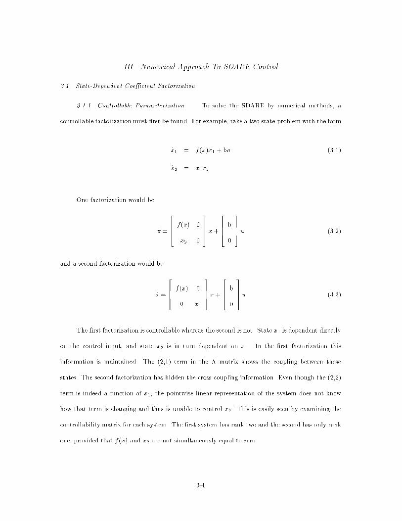
3.1.1 Controllable Parameterization. To solve the SDARE by numerical methods, a
controllable factorization must �rst be found. For example, take a two state problem with the form
_x1 = f(x)x1 + bu (3.1)
_x2 = x1x2
One factorization would be
_x =
2664 f(x) 0
x2 0
3775x+
2664 b
0
3775u (3.2)
and a second factorization would be
_x =
2664 f(x) 0
0 x1
3775x+
2664 b
0
3775u (3.3)
The �rst factorization is controllable whereas the second is not. State x1 is dependent directly
on the control input, and state x2 is in turn dependent on x1. In the �rst factorization this
information is maintained. The (2,1) term in the A matrix shows the coupling between these
states. The second factorization has hidden the cross coupling information. Even though the (2,2)
term is indeed a function of x1, the pointwise linear representation of the system does not know
how that term is changing and thus is unable to control x2. This is easily seen by examining the
controllability matrix for each system. The �rst system has rank two and the second has only rank
one, provided that f(x) and x2 are not simultaneously equal to zero.
3-1

3.1.2 Optimal Parameterizations. Di�erent factorizations of the same problem can have
di�erent control histories. When examining a �xed parameterization to solve the SDARE, any
given SDC choice will not necessarily be optimal. To establish optimality, Cloutier, et al. estab-
lish a parameterization set which spans a hyperplane of possible solution parameterizations using
spanning variables f�ig. To achieve this optimality, each f�ig must be solved for as a function of
time which involves solving a two point boundary value problem.
However, a numerical approach using a �xed suboptimal SDC choice can provide insight
into increasingly complex systems for which �nding the positive de�nite solution with associated
boundary conditions is not a trivial undertaking. It is not implied that any factorization in the
following chapters is the optimal solution. Chapter V will show variations in control usage between
two parameterizations with equal weighting functions. One parameterization might be more nearly
optimal than the other, but it might just take changing the Q and R weightings to create a practical
solution. Also, from an implementation point of view, optimality might not be signi�cant. Any
stabilizable and detectable parameterization will achieve the same �nal result, i.e. perturbed states
will return to zero. If the state or control deviations or settling time are unacceptable no matter
what the Q and R weights are, then pursuing an optimal solution will most likely be necessary.
3.1.3 Ill-Conditioned Parameterizations. Numerical problems can arise when one state
di�erential equation is parameterized in a way which is nearly the same as another, i.e., a multiple
of the other. This is best seen using a real example, which will be illustrated in Section 6.3.1, Eqn.
(6.10). Further discussion of this issue will be deferred to that section.
3.2 Numerical Implementation
All simulations in this thesis were accomplished using MATLAB and SIMULINK [MAT].
One function contained the nonlinear di�erential equations. A second function created the A, B,
Q, and R matrices of the SDC parameterizations. At each time step, the state dependent algebraic
3-2
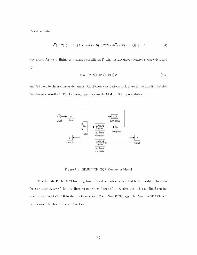
Riccati equation
AT (x)P (x) + P (x)A(x)� P (x)B(x)R�1(x)BT (x)P (x) + Q(x) = 0 (3.4)
was solved for a stabilizing or neutrally stabilizing P. The instantaneous control u was calculated
by
u = �R�1(x)BT (x)P (x)x (3.5)
and fed back to the nonlinear dynamics. All of these calculations took place in the function labeled
\nonlinear controller". The following �gure shows the SIMULINK representation.
Mux
Mux
MATLABFunction
nonlinearcontroller
MATLABFunction
nonlineardynamics
1/sIntegrator
xdot
derivatives
x
states
u
controls
Clock
tmtime
Figure 3.1 SIMULINK NQR Controller Model
To calculate P, the MATLAB algebraic Riccati equation solver had to be modi�ed to allow
for zero eigenvalues of the Hamiltonian matrix as discussed in Section 2.5. This modi�ed routine
was invoked in MATLAB in the the form SDARE(A, B*inv(R)*B', Q). The function SDARE will
be discussed further in the next section.
3-3

3.3 Numerical Issues
3.3.1 Zero Eigenvalue Pairs. An interesting problem arose in the simulations of satellite
attitude control. Originally set up using Euler angles, it was suggested by Hall [Hal95a] that
they be examined using quaternions since that is the more standard coordinate system. Because
quaternions describe 3 space with 4 parameters, there is an inherent constraint. Due to this
constraint, the associated Hamiltonian of the SDARE will have a zero eigenvalue pair, because of
symmetry, implying a nonstabilizable mode, i.e. the constraint itself. However, if the nature of this
nonstabilizable mode is something we can neglect, we can construct a neutrally stabilizing solution
and use it.
Our goal in nonlinear quadratic regulation is to drive the state deviations and control usage
to zero. If we have a constrained state as above, it may only be possible to drive all but one state
to zero. The last state will settle at a non-zero value, consistent with its zero eigenvalue. This
state should be left unweighted and therefore undetectable. This prevents its inclusion in the cost
function, which would otherwise be in�nite. If the value the unconstrained state will settle at is
known and acceptable, then the neutrally stabilizing solution to the SDARE is acceptable.
This can result in fairly e�ective controllers; however, there is one precaution. If there is
more than one solution to the constrained states, there is no guarantee that the unweighted state
will go to the desired solution. As a regulator this could pose a problem when a disturbance is
large enough to move the states into the vicinity of the other solutions. In this sense the system is
not completely controllable to the desired equilibrium. For example, take a two state vector that
is constrained to have magnitude of 1, and you wish to keep it in an equilibrium value of [0 1]T by
penalizing only the �rst state. Starting from equilibrium the controller might work �ne. If however,
the states are disturbed to a value close to [0 �1]T , the controller will probably then drive the �rst
state to zero leaving the second state at its new value. The system will now be regulated about
this undesired equilibrium.
3-4
The standard MATLAB algebraic Riccati equation solver is designed to return only stabilizing
solutions. Because we are now interested in neutrally stabilizing solutions as well, the function
ARE(a,b,c) was altered into a new function SDARE(a,b,c). This was done by eliminating the error
checking routine which checked for n negative eigenvalues. The eigenvectors are sorted by their
respective eigenvalue sign from negative to zero and then positive. The modi�ed routine would now
return a neutrally stabilizing solution because it used the eigenvector associated with an imaginary
axis eigenvalue. Admittedly, this is not a robust error checking method, but it worked for the
satellite examples examined. More coding and error checking would have to be done for the routine
to be used on any example. The pancreas dynamics required only the standard ARE solver.
3.3.2 Singularity. A problem can be factored into a form where there is division by any
one of the states. This is numerically disastrous as the states approach zero. For a problem as
complex as the pancreas in Chapter VII, this factorization may be unavoidable. If so, it may be
necessary to introduce a dead band where the states are nearly zero and no control is used since
the states are su�ciently close to zero. This deadband was introduced into the controller for the
arti�cial pancreas, because of division by the glucose state. The numerics were well behaved for
very small values of the glucose state, so a deadband for values less than 0.0001 only was used.
This is su�ciently close to our desired value and results in no performance loss.
3-5

IV. Satellite Dynamics
This chapter gives the simpli�ed satellite dynamics for the problems considered in this thesis,
and then incorporates those dynamics into a state dependent coe�cient form.
The notation kvk will be used to denote the Euclidean norm of a vector; i.e., its magnitude.
4.1 Rigid Body with 3-axis External Torques
Assuming a rigid body, a satellite controlled with external torques obeys Euler's equation
given by
_! = �J�1! � J! + J�1T (4.1)
where ! is the body axis angular velocity vector, J is the inertia tensor, and T is the external
torques about each body axis. The derivation of rigid body motion can be found in most dynamics
texts. A good reference is Chobotov [Cho91], which concentrates speci�cally on satellites.
4.2 Rigid Body with Internal Stabilizing Rotors
Another interesting problem we will examine for which nonlinear quadratic regulation could
have practical application is a satellite stabilized by internal spinning rotors. The internal rotors
provide not only stability, but by changing the angular rates of each rotor, the satellite can be
brought to a new orientation. The total angular momentum of the satellite will be constant since
no external forces are present.
We will de�ne the vector �, containing three states, to have elements representing the axial
angular momentum of each rotor relative to inertial space. The vector x, also containing three
states, is the angular momentum expressed in body axes and is scaled such that kxk = 1. The
control vector u will be the torque applied to each rotor. The system dynamics are
4-1
_� = u (4.2)
_x = x� J�1(x� A�) (4.3)
Given n rotors (controllers), then � 2 Rn, u 2 Rn, x 2 R3, J 2 R3�3, and A 2 R3�n. J is a scaled
inertia tensor given by
J = Jsat � ATJrotA (4.4)
where Jsat is the satellite inertia tensor, and Jrot is a diagonal n � n matrix with elements cor-
responding to each rotor's inertia. The matrix A has columns of unit vectors representing the
direction of each rotor's axis of spin in body axes, and whose order corresponds to the order of Jrot.
The equations of motion for this section were developed by Hall [Hal95b]. Leaving the notation the
same unfortunately leads to another use of A and x. Since these variables will appear as elements
of A(x)x their meaning should be taken from context.
We will also need the angular rates, !, given by
! = J�1(x� A�) (4.5)
Notice the satellite is stationary when x = A�. Also note that Eqn. (4.3) can be simply written as
_x = x� !.
4.3 Attitude Coordinates
The above sections give the equations for body axis angular rates. If in addition to angular
velocities we want to regulate an inertial position, then we must also include an inertial coordinate
system. To express the orientation of the satellite there are several options. Euler angles are
a common representation, but because the equation of motions can become singular for certain
4-2
angles, quaternions are a preferable coordinate system. Initial quaternion values can be found from
the initial rotation matrix.
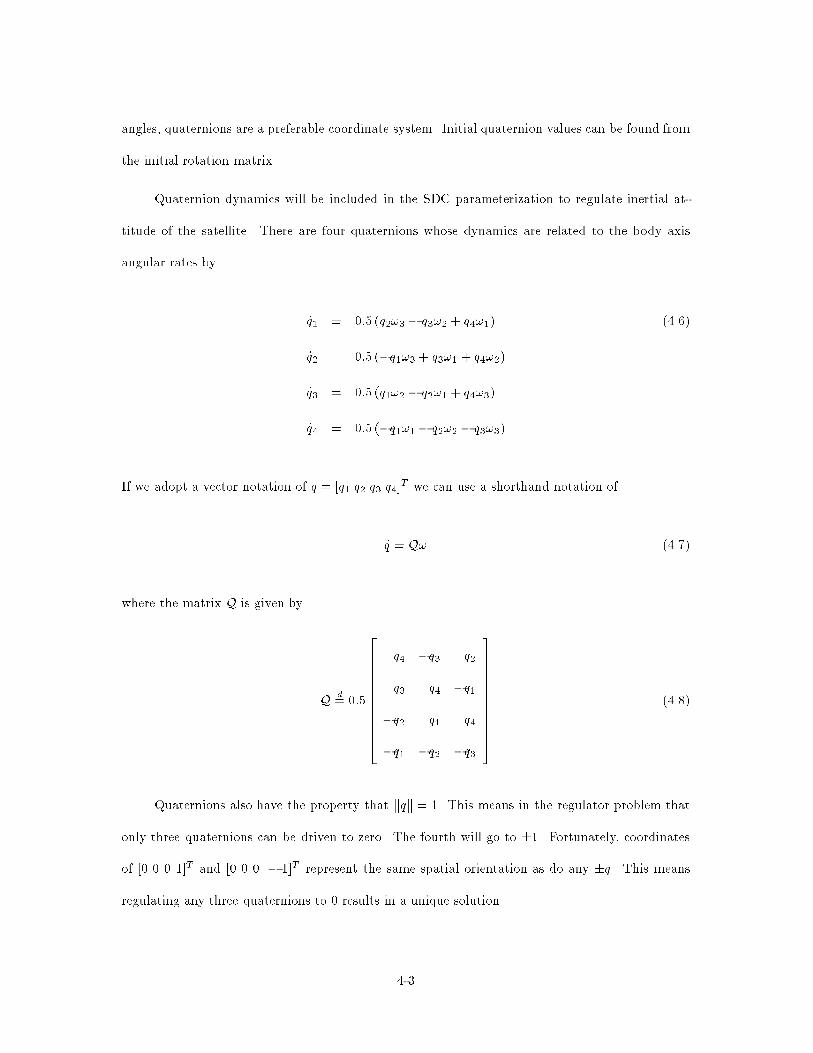
Quaternion dynamics will be included in the SDC parameterization to regulate inertial at-
titude of the satellite. There are four quaternions whose dynamics are related to the body axis
angular rates by
_q1 = 0:5 (q2!3 � q3!2 + q4!1) (4.6)
_q2 = 0:5 (�q1!3 + q3!1 + q4!2)
_q3 = 0:5 (q1!2 � q2!1 + q4!3)
_q4 = 0:5 (�q1!1 � q2!2 � q3!3)
If we adopt a vector notation of q = [q1 q2 q3 q4]T we can use a shorthand notation of
_q = Q! (4.7)
where the matrix Q is given by
Qd= 0:5
266666666664
q4 �q3 q2
q3 q4 �q1
�q2 q1 q4
�q1 �q2 �q3
377777777775
(4.8)
Quaternions also have the property that kqk = 1. This means in the regulator problem that
only three quaternions can be driven to zero. The fourth will go to �1. Fortunately, coordinates
of [0 0 0 1]T and [0 0 0 � 1]T represent the same spatial orientation as do any �q. This means
regulating any three quaternions to 0 results in a unique solution.
4-3
As we shall see later, the properties of quaternions result in a rank defective controllability
matrix. This would appear to cause problems; however, we will be able to use the neutrally
stabilizing solution to the SDARE as discussed previously.
There are several di�erent ways quaternions can be de�ned. The quaternions used in this
thesis are the same as found in Chobotov [Cho91].
4.4 Cross Product Notation
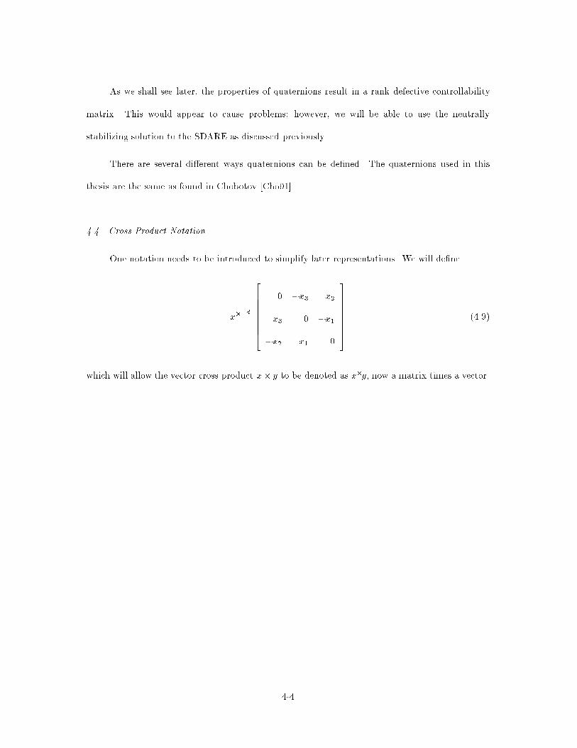
One notation needs to be introduced to simplify later representations. We will de�ne
x�d=
26666664
0 �x3 x2
x3 0 �x1
�x2 x1 0
37777775
(4.9)
which will allow the vector cross product x� y to be denoted as x�y, now a matrix times a vector.
4-4
V. Suboptimal SDC Controllers
This chapter provides a conceptual feel for both how to choose a �xed SDC parameterization,
and how optimality can impact performance.
5.1 SDC Parameterization
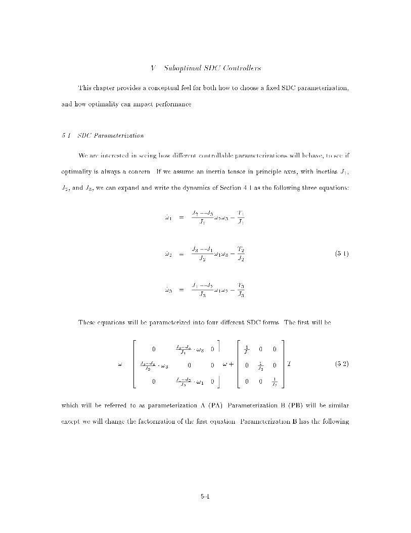
We are interested in seeing how di�erent controllable parameterizations will behave, to see if
optimality is always a concern. If we assume an inertia tensor in principle axes, with inertias J1,
J2, and J3, we can expand and write the dynamics of Section 4.1 as the following three equations:
_!1 =J2 � J3
J1!2!3 +
T1
J1
_!2 =J3 � J1
J2!1!3 +
T2
J2(5.1)
_!3 =J1 � J2
J3!1!2 +
T3
J3
These equations will be parameterized into four di�erent SDC forms. The �rst will be
_! =
26666664
0 J2�J3J1
� !3 0
J3�J1J2
� !3 0 0
0 J1�J2J3
� !1 0
37777775! +
26666664
1J1
0 0
0 1J2
0
0 0 1J3
37777775T (5.2)
which will be referred to as parameterization A (PA). Parameterization B (PB) will be similar
except we will change the factorization of the �rst equation. Parameterization B has the following
5-1
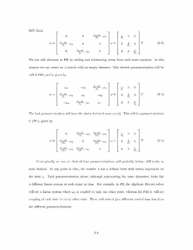
SDC form
_! =
26666664
0 0 J2�J3J1
� !2
J3�J1J2
� !3 0 0
0 J1�J2J3
� !1 0
37777775! +
26666664
1J1
0 0
0 1J2
0
0 0 1J3
37777775T (5.3)
We can add elements to PB by adding and subtracting terms from each state equation. In this
manner we can create an A matrix with no empty elements. This altered parameterization will be
called PB2, and is given by
_! =
26666664
!2 �!1J2�J3J1
� !2
J3�J1J2
� !3 !3 �!2
�!3J1�J2J3
� !1 !1
37777775! +
26666664
1J1
0 0
0 1J2
0
0 0 1J3
37777775T (5.4)
The last parameterization will have the states factored more evenly. This will be parameterization
C (PC), given by
_! =
26666664
0 J2�J32J1
� !3J2�J32J1
� !2
J3�J12J2
� !3 0 J3�J12J2
� !1
J1�J22J3
� !2J1�J22J3
� !1 0
37777775! +
26666664
1J1
0 0
0 1J2
0
0 0 1J3
37777775T (5.5)
Conceptually we can see that all four parameterizations will probably behave di�erently in
some fashion. At any point in time, the matrix A has a de�nite form with values dependent on
the state !. Each parameterization above, although representing the same dynamics, looks like
a di�erent linear system at each point in time. For example, in PA the algebraic Riccati solver
will see a linear system where !3 is coupled to only one other state, whereas for PB2 it will see
coupling of each state to every other state. These will indeed give di�erent control laws based on
the di�erent parameterizations.
5-2
5.2 Results
Now let's examine how each model performs in a numerical simulation. We will use an inertia
matrix of
J =
26666664
10 0 0
0 15 0
0 0 20
37777775
(5.6)
All control simulations for this chapter will have initial angular velocities of
!0 =
26666664
4
4
2
37777775
(5.7)
To compare all four factorizations we will use a state penalty weight of Q = 10I3�3 and a
control penalty weight of R = I3�3. The results of parameterization A can be seen in Figures
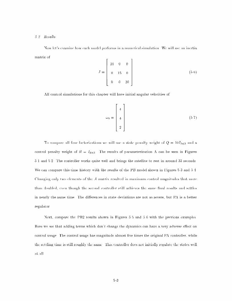
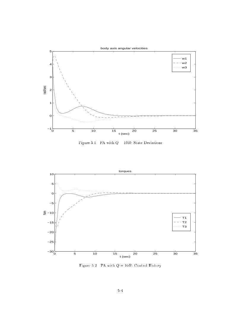
5.1 and 5.2. The controller works quite well and brings the satellite to rest in around 35 seconds.
We can compare this time history with the results of the PB model shown in Figures 5.3 and 5.4.
Changing only two elements of the A matrix resulted in maximum control magnitudes that more
than doubled, even though the second controller still achieves the same �nal results and settles
in nearly the same time. The di�erences in state deviations are not as severe, but PA is a better
regulator.
Next, compare the PB2 results shown in Figures 5.5 and 5.6 with the previous examples.
Here we see that adding terms which don't change the dynamics can have a very adverse e�ect on
control usage. The control usage has magnitude almost �ve times the original PA controller, while
the settling time is still roughly the same. This controller does not initially regulate the states well
at all.
5-3
w1
w2
w3
0 5 10 15 20 25 30 35−1
0
1
2
3
4
5body axis angular velocities
t (sec)
rad/s
ec
Figure 5.1 PA with Q = 10R: State Deviations
T1
T2
T3
0 5 10 15 20 25 30 35−30
−25
−20
−15
−10
−5
0
5
10torques
t (sec)
Nm
Figure 5.2 PA with Q = 10R: Control History
5-4
w1
w2
w3
0 5 10 15 20 25 30 35−2
−1
0
1
2
3
4
5body axis angular velocities
t (sec)
rad/s
ec
Figure 5.3 PB with Q = 10R: State Deviations
T1
T2
T3
0 5 10 15 20 25 30 35−80
−60
−40
−20
0
20
40
60torques
t (sec)
Nm
Figure 5.4 PB with Q = 10R: Control History
5-5

w1
w2
w3
0 5 10 15 20 25 30 35−1
−0.5
0
0.5
1
1.5
2
2.5
3
3.5
4body axis angular velocities
t (sec)
rad/
sec
Figure 5.5 PB2 with Q = 10R: State Deviations
T1
T2
T3
0 5 10 15 20 25 30 35−150
−100
−50
0
50
100
150torques
t (sec)
Nm
Figure 5.6 PB2 with Q = 10R: Control History
5-6
w1
w2
w3
0 5 10 15 20 25 30 35−1
0
1
2
3
4
5body axis angular velocities
t (sec)
rad/s
ec
Figure 5.7 PC with Q = 10R: State Deviations
T1
T2
T3
0 5 10 15 20 25 30 35−30
−25
−20
−15
−10
−5
0
5
10torques
t (sec)
Nm
Figure 5.8 PC with Q = 10R: Control History
5-7
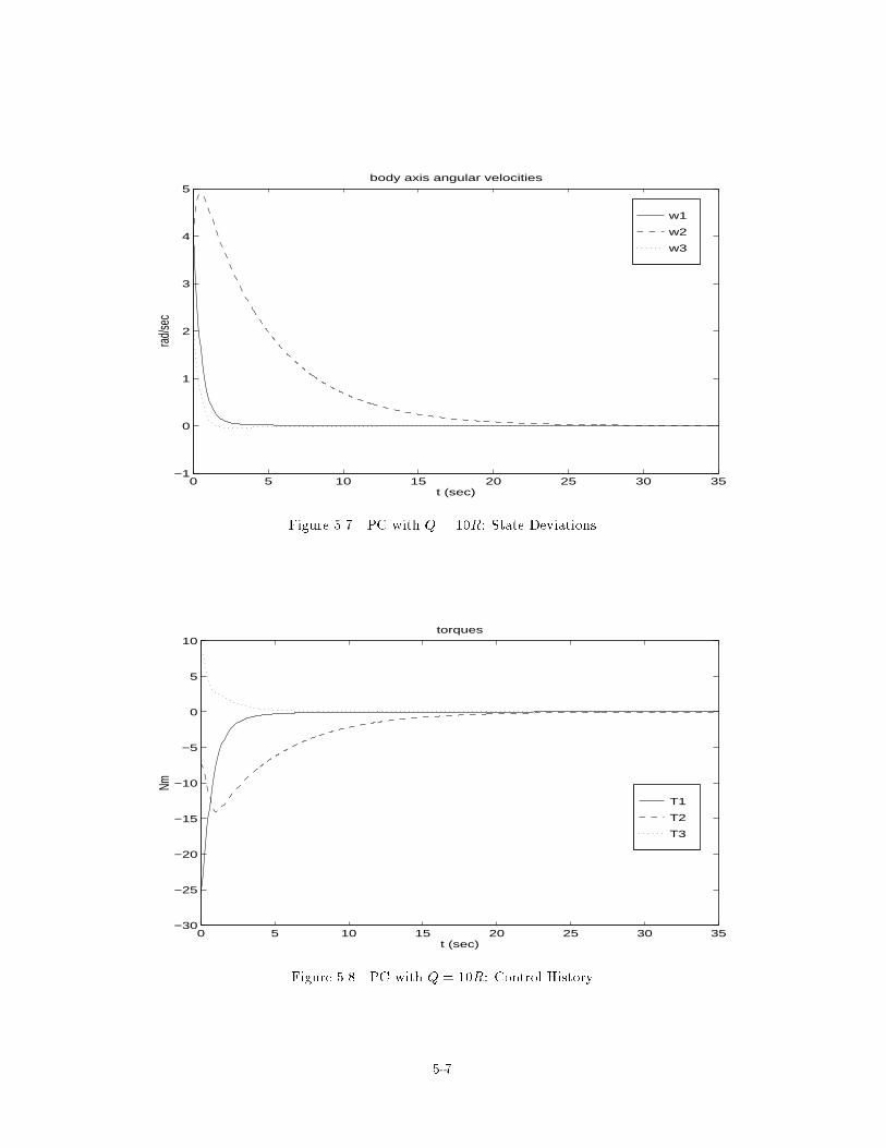
The last SDC form, PC, gives a controller with the results seen in Figures 5.7 and 5.8. This
controller produces considerably smoother time histories with maximum control magnitudes less
than all previous SDC forms. The �rst and third angular velocities are regulated very quickly; the
second is much slower, but still settles in the same amount of time as the previous controllers. This
is an excellent regulator, especially if !2 is not as critical. Increasing state weighting will bring !2
back to equilibrium quicker, but at the cost of more control usage.
We can evaluate the cost function associated with each parameterization using numerical
integration. Using a trapezoidal approximation, the cost functions were 1:71e + 3, 3:35e + 3,
1:19e+4, and 1:73e+3 respectively. Since parameterizations A and C had the closest performance
of the four forms examined, we will now see how di�erent weightings a�ect these two controllers.
The next simulations will have state weighting of Q = I and control weighting of R = 10I.
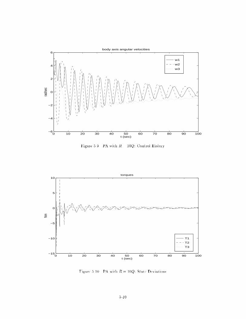
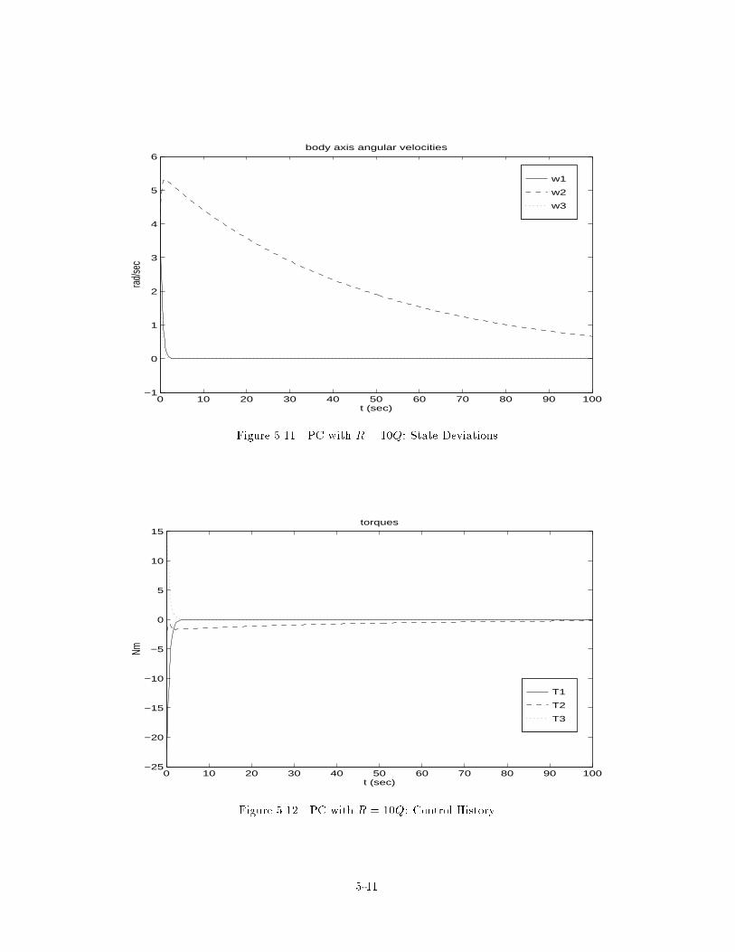
Figures 5.9 and 5.10 show PA's performance, and PC's performance is shown in Figures 5.11
and 5.12. Here the performance is considerably di�erent. Parameterization A has a more rapidly
changing control usage. The state deviations and control usage are oscillatory as compared to the
still exponential nature of parameterization C. Time to settle for both controllers is around �ve
minutes. Parameterization A now has a cost function of 2:07e + 3 while PC's cost function is
4:46e + 3. Here we can see that although one parameterization is more optimal than another, it
may not necessarily have desirable characteristics.
Figures 5.13 and 5.14 show parameterization C with an even larger control penalty of R =
105I. Notice that !1 and !3 still have the same behavior, while !2 is directly related to the control
weighting. Parameterization C tries to stop the tumbling motion of the satellite as quickly as
possible, and then brings the third state to rest at a rate directly related to control weighting.
We will examine one last simulation. Since parameterization C has maximum control magni-
tudes that are almost invariant to changes in the penalty matrices Q and R, we will see if limiting
control usage still results in a stable controller. Figures 5.15 and 5.16 show the results of parameter-
5-8
ization C using the original weights of the �rst example, except that control usage is sent through
a limiter of �2 Nm. Notice that the controller uses maximum control until the state deviations are
reduced to a level where the control exponentially dies out. The controller is still quite e�ective
even though the reduction in control usage could not be accomplished by control weighting.
5.3 Summary
We have seen that di�erences between factorizations produce di�erent state and control histo-
ries, and can be very sensitive to state and control weightings. For the examples considered, heavy
control penalties greatly enlarged the di�erences between parameterizations A and C, which had
relatively similar performance under heavy state weighting. We also saw that although relatively
little changes in the A matrix could e�ect the control and state histories, there was little change in
�nal settling time.
Adding elements to the A matrix so that dynamics cancel out is a trick used by Cloutier,
et al., [CDM95] for a system that has a zero A matrix. In the example here, it was seen that
there were adverse e�ects from adding those terms to an A matrix that was already well behaved.
Adding terms should probably only be done to handle such special cases like the one examined in
[CDM95].
Conceptually, we have learned a little about forming a good state dependent coe�cient fac-
torization for a given system. Of the four parameterizations examined, parameterization C appears
to give the overall better performance. It di�ers from the other parameterizations in that its dy-
namics are more evenly distributed among all the terms. State Dependent Coe�cient form is a way
to make a nonlinear system look linear at each point in time. By distributing the dynamics, the
linear representation shows all the coupling between states and their relationships to one another.
Therefore, a nonlinear term like x1x2x3 might be better represented by dividing it in thirds and
factoring out each state, rather than factoring one state and leaving the rest as a single coe�cient.
5-9
w1
w2
w3
0 10 20 30 40 50 60 70 80 90 100−6
−4
−2
0
2
4
6body axis angular velocities
t (sec)
rad/s
ec
Figure 5.9 PA with R = 10Q: Control History
T1
T2
T3
0 10 20 30 40 50 60 70 80 90 100−15
−10
−5
0
5
10torques
t (sec)
Nm
Figure 5.10 PA with R = 10Q: State Deviations
5-10
w1
w2
w3
0 10 20 30 40 50 60 70 80 90 100−1
0
1
2
3
4
5
6body axis angular velocities
t (sec)
rad/s
ec
Figure 5.11 PC with R = 10Q: State Deviations
T1
T2
T3
0 10 20 30 40 50 60 70 80 90 100−25
−20
−15
−10
−5
0
5
10
15torques
t (sec)
Nm
Figure 5.12 PC with R = 10Q: Control History
5-11
w1
w2
w3
0 10 20 30 40 50 60 70 80 90 100−1
0
1
2
3
4
5
6body axis angular velocities
t (sec)
rad/s
ec
Figure 5.13 PC with R = 105Q: State Deviations
T1
T2
T3
0 10 20 30 40 50 60 70 80 90 100−25
−20
−15
−10
−5
0
5
10
15torques
t (sec)
Nm
Figure 5.14 PC with R = 105Q: Control History
5-12
w1
w2
w3
0 10 20 30 40 50 60−6
−4
−2
0
2
4
6body axis angular velocities
t (sec)
rad/s
ec
Figure 5.15 PC with Q = 10R, maxjuij = 2: State Deviations
T1
T2
T3
0 10 20 30 40 50 60−3
−2
−1
0
1
2
3torques
t (sec)
Nm
Figure 5.16 PC with Q = 10R, maxjuij = 2: Control History
5-13
The importance of optimality depends on each control problem examined. For our examples,
each �xed sub-optimal parameterization resulted in an e�ective controller. If the control usage
was too high for what would be implemented, the control could be limited. Implementing and
testing a �xed SDC form was relatively quick, and many permutations of penalty matrices could be
evaluated. If none of the controllers provided acceptable state and control histories, then at least
the insight gained from the �xed form could help in choosing penalty matrices before solving the
optimal problem.
5-14
VI. Satellite Control Results
This chapter will show the e�ectiveness of the numerical SDARE solutions using the dynam-
ics of Chapter IV. The two examples presented here provide more practical examples than the
illustrative problem of Chapter V.
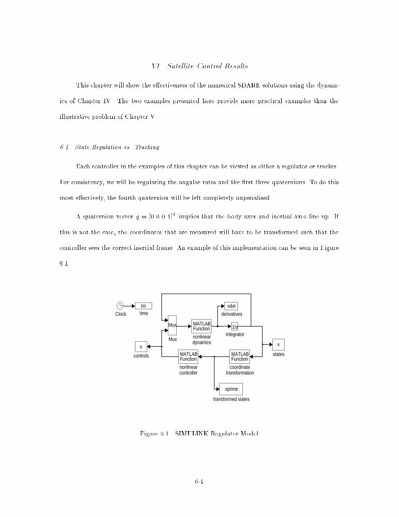
6.1 State Regulation vs. Tracking
Each controller in the examples of this chapter can be viewed as either a regulator or tracker.
For consistency, we will be regulating the angular rates and the �rst three quaternions. To do this
most e�ectively, the fourth quaternion will be left completely unpenalized.
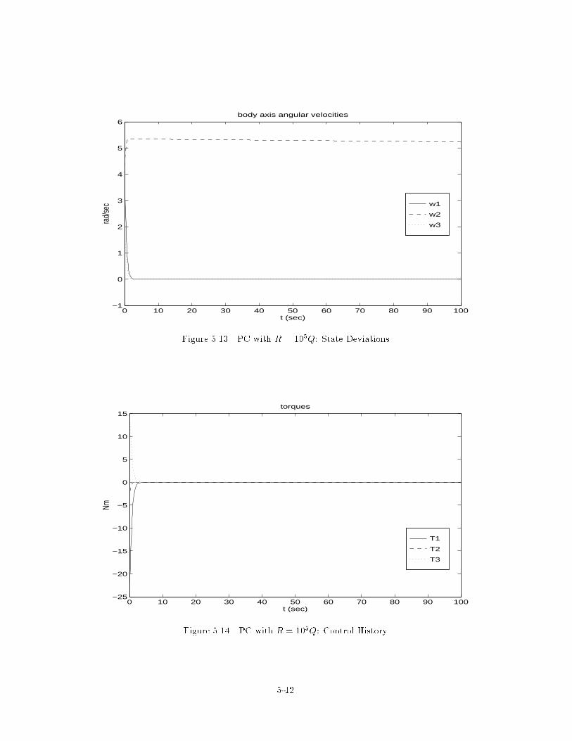
A quaternion vector q = [0 0 0 1]T implies that the body axes and inertial axes line up. If
this is not the case, the coordinates that are measured will have to be transformed such that the
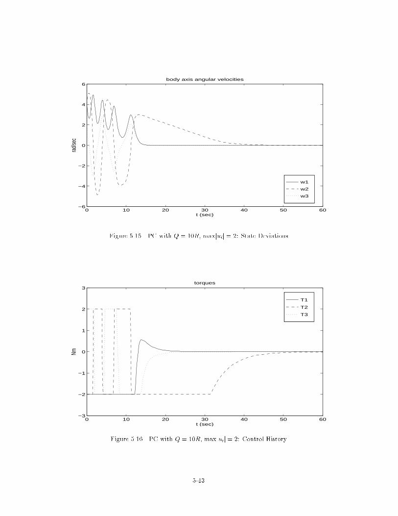
controller sees the correct inertial frame. An example of this implementation can be seen in Figure
6.1.
Mux
Mux
MATLABFunction
nonlineardynamics
1/sIntegrator
xdot
derivatives
u
controls
Clock
tmtime
MATLABFunction
nonlinearcontroller
MATLABFunction
coordinatetransformation
xprime
transformed states
x
states
Figure 6.1 SIMULINK Regulator Model
6-1
In this same manner, the regulator can be made a tracker. To reorient the satellite, a di�erent
coordinate transformation merely needs to be done on the measured coordinates and then fed to
the controller. To accomplish this, the quaternions would be transformed to a rotation matrix, then
multiplied by the coordinate transformation. From this �nal rotation matrix the new quaternions
can be calculated.
For systems whose states can all be driven to an equilibrium value, the coordinate transfor-
mation is not as complex. The tracking diagram for the pancreas model in Chapter VIII shows the
more familiar method of subtracting reference values from the actual state values.
6.2 Despin of Satellite Using External Torques
This section will look at the following problem: given a perturbed rotating satellite, bring it
to rest in a speci�c orientation.
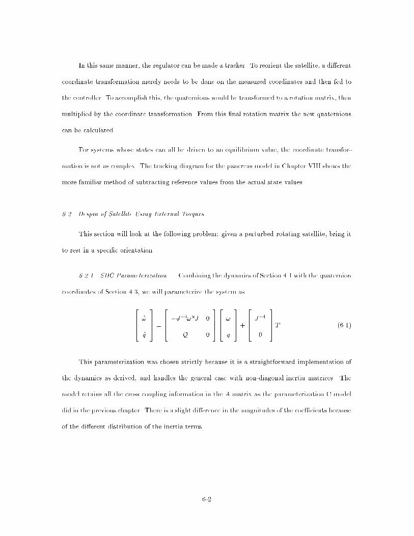
6.2.1 SDC Parameterization. Combining the dynamics of Section 4.1 with the quaternion
coordinates of Section 4.3, we will parameterize the system as
2664 _!
_q
3775 =
2664 �J�1!�J 0
Q 0
37752664 !
q
3775+
2664 J�1
0
3775T (6.1)
This parameterization was chosen strictly because it is a straightforward implementation of
the dynamics as derived, and handles the general case with non-diagonal inertia matrices. The
model retains all the cross coupling information in the A matrix as the parameterization C model
did in the previous chapter. There is a slight di�erence in the magnitudes of the coe�cients because
of the di�erent distribution of the inertia terms.
6-2
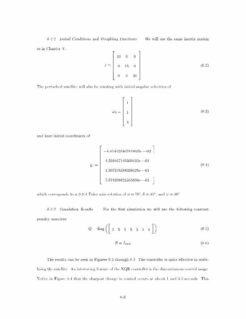
6.2.2 Initial Conditions and Weighting Functions. We will use the same inertia matrix
as in Chapter V,
J =
26666664
10 0 0
0 15 0
0 0 20
37777775
(6.2)
The perturbed satellite will also be rotating with initial angular velocities of
!0 =
26666664
1
1
4
37777775
(6.3)
and have initial coordinates of
q0 =
266666666664
�1:614529367818635e� 02
4:399467145509192e� 01
4:307255588328425e� 01
7:878208621355699e� 01
377777777775
(6.4)
which corresponds to a 3-2-1 Euler axis rotation of � = 70o; � = 45o, and = 30o.
6.2.3 Simulation Results. For the �rst simulation we will use the following constant
penalty matrices:
Q = diag
��5 5 5 5 5 5 0
��(6.5)
R = I3�3 (6.6)
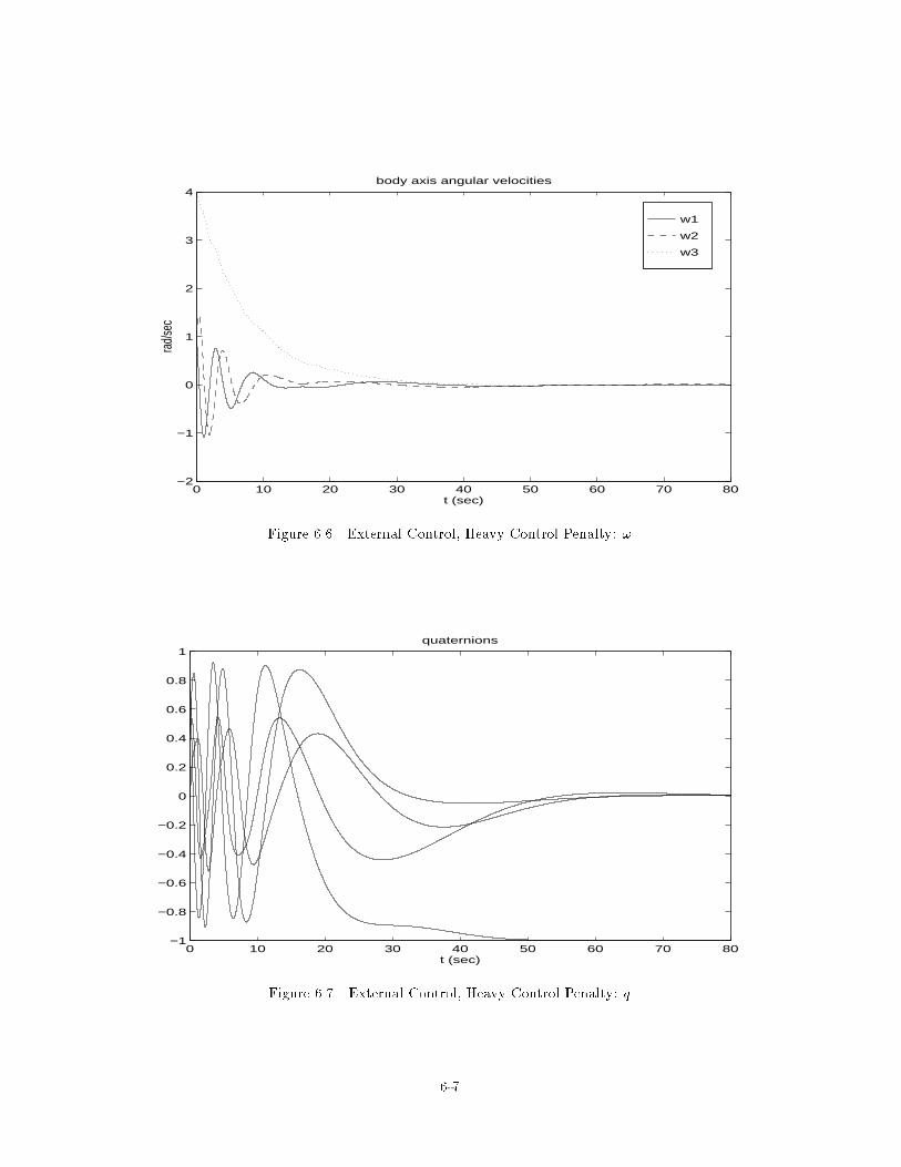
The results can be seen in Figures 6.2 through 6.5. The controller is quite e�ective in stabi-
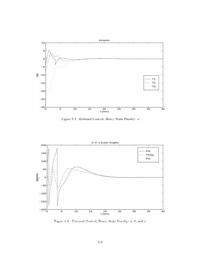
lizing the satellite. An interesting feature of the NQR controller is the discontinuous control usage.
Notice in Figure 6.4 that the sharpest change in control occurs at about 1 and 3.5 seconds. This
6-3
corresponds to where the unweighted quaternion q4 is zero, which is also where � takes its largest
value.
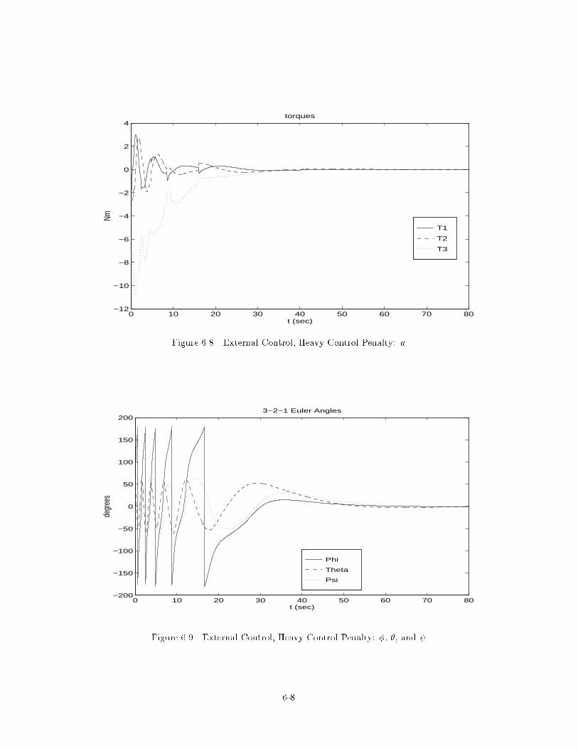
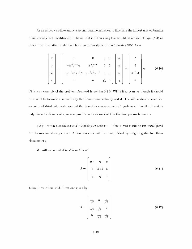
For comparison, we will do a second simulation using the following constant penalty matrices:
Q = diag
��1 1 1 1 1 1 0
��(6.7)
R = 5I3�3 (6.8)
The results of the second weighting can be seen in Figures 6.6 through 6.9. This controller
behaves as we would expect it to. With the reduced control usage, it takes almost twice as long
to stabilize. The behavior is more oscillatory since the satellite will undergo more rotations during
the regulation process. What is interesting to note here is that the unweighted quaternion q4 went
to �1, unlike +1 in the previous simulation, yet the �nal orientation of the satellite is the same.
This con�rms that we can pose a \stabilizable" problem, even though we had a nonstabilizable
Hamiltonian matrix.
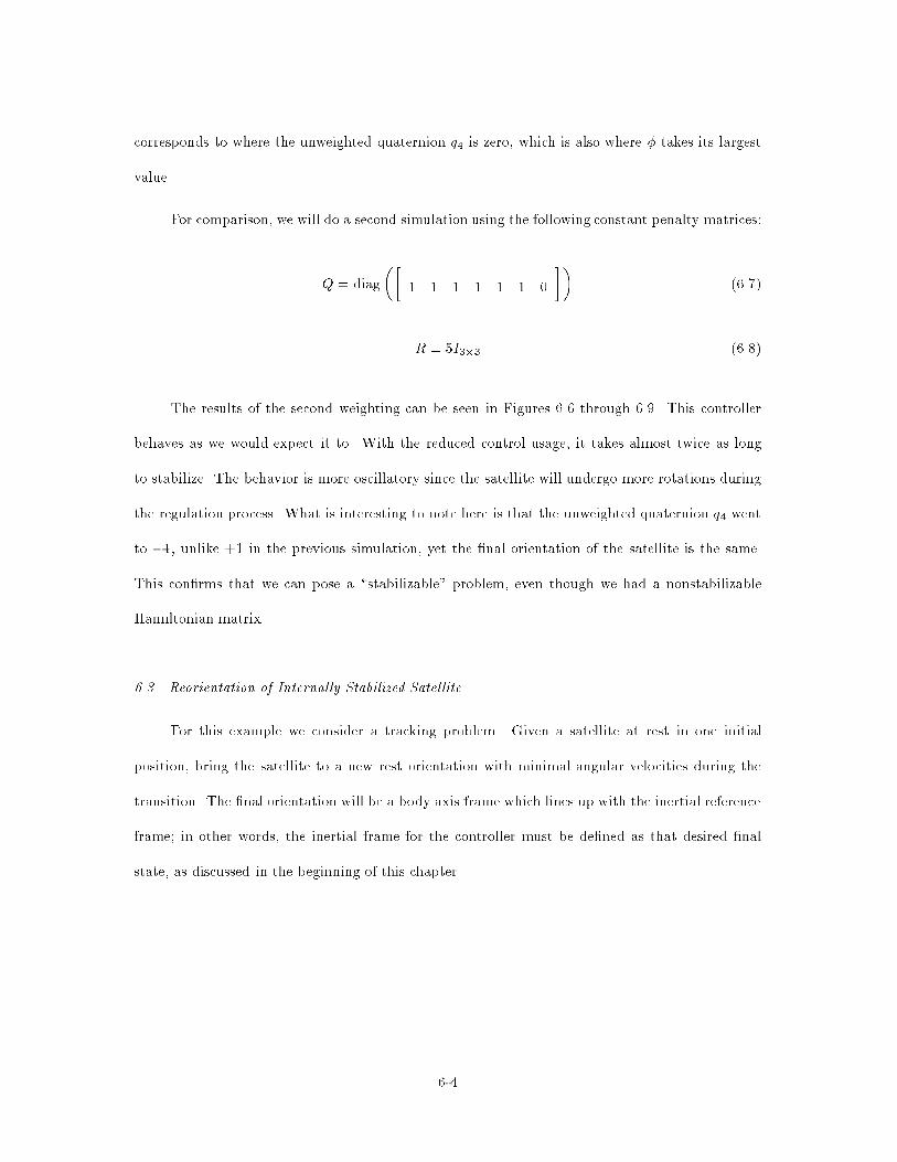
6.3 Reorientation of Internally Stabilized Satellite
For this example we consider a tracking problem. Given a satellite at rest in one initial
position, bring the satellite to a new rest orientation with minimal angular velocities during the
transition. The �nal orientation will be a body axis frame which lines up with the inertial reference
frame; in other words, the inertial frame for the controller must be de�ned as that desired �nal
state, as discussed in the beginning of this chapter.
6-4
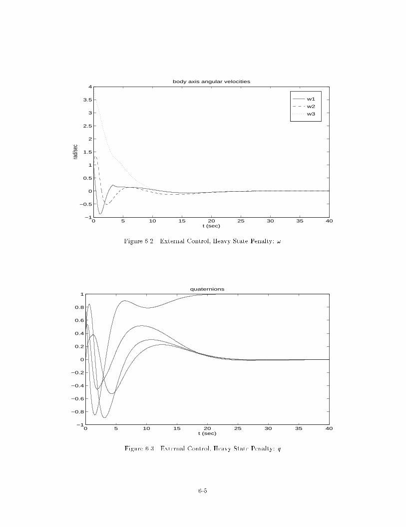
w1
w2
w3
0 5 10 15 20 25 30 35 40−1
−0.5
0
0.5
1
1.5
2
2.5
3
3.5
4body axis angular velocities
t (sec)
rad/
sec
Figure 6.2 External Control, Heavy State Penalty: !
0 5 10 15 20 25 30 35 40−1
−0.8
−0.6
−0.4
−0.2
0
0.2
0.4
0.6
0.8
1quaternions
t (sec)
Figure 6.3 External Control, Heavy State Penalty: q
6-5
T1
T2
T3
0 5 10 15 20 25 30 35 40−30
−25
−20
−15
−10
−5
0
5
10torques
t (sec)
Nm
Figure 6.4 External Control, Heavy State Penalty: u
Phi
Theta
Psi
0 5 10 15 20 25 30 35 40−200
−150
−100
−50
0
50
100
150
2003−2−1 Euler Angles
t (sec)
degr
ees
Figure 6.5 External Control, Heavy State Penalty: �, �, and
6-6
w1
w2
w3
0 10 20 30 40 50 60 70 80−2
−1
0
1
2
3
4body axis angular velocities
t (sec)
rad/s
ec
Figure 6.6 External Control, Heavy Control Penalty: !
0 10 20 30 40 50 60 70 80−1
−0.8
−0.6
−0.4
−0.2
0
0.2
0.4
0.6
0.8
1quaternions
t (sec)
Figure 6.7 External Control, Heavy Control Penalty: q
6-7
T1
T2
T3
0 10 20 30 40 50 60 70 80−12
−10
−8
−6
−4
−2
0
2
4torques
t (sec)
Nm
Figure 6.8 External Control, Heavy Control Penalty: u
Phi
Theta
Psi
0 10 20 30 40 50 60 70 80−200
−150
−100
−50
0
50
100
150
2003−2−1 Euler Angles
t (sec)
degr
ees
Figure 6.9 External Control, Heavy Control Penalty: �, �, and
6-8

6.3.1 SDC Parameterization. Using the dynamics of Section 4.2 and di�erentiating Eqn.
(4.5), we can form the following SDC factorization
266666666664
_�
_x
_!
_q
377777777775=
266666666664
0 0 0 0
0 0 x� 0
�J�1x�J�1A J�1x�J�1 0 0
0 0 Q 0
377777777775
266666666664
�
x
!
q
377777777775+
266666666664
I
0
J�1A
0
377777777775u (6.9)
remembering that � is each rotor's angular momentum expressed in body axes, and x is the scaled
angular momentum of the entire satellite expressed in body coordinates. For our examples, � and
x are three dimensional vectors.
This factorization is rather large and has some advantages and disadvantages associated with
it. With this form, both angular rates and positions can be regulated and penalized accordingly.
This SDC form does, however, contain redundant information; i.e., specifying the quaternions will
uniquely de�ne the body axis momentum. This parameterization expresses the dynamics more
e�ciently using the state x.
It is important to notice that the state � is not desired to be regulated to zero, since it is the
rotors' angular rates that will keep the satellite stationary. Therefore, � should be left unpenalized
and thus undetectable.
Satellite attitude is best regulated through q, and therefore x should also be unweighted. The
reason x is not a good choice for attitude control, even though it is an inertially constant vector,
involves the constraint kxk = 1. Like q, we could choose to make all but one coordinate go to zero.
This is easily done; however, unlike q the position of the satellite is not uniquely de�ned in two
senses. The xn which is unweighted can go to either +1 or �1, which are indeed di�erent answers.
Also, even if x did achieve the desired �nal values, this only guarantees that the body vector and
inertial vector are colinear. There is no unique rotation of the satellite about that axis.
6-9
As an aside, we will examine a second parameterization to illustrate the importance of forming
a numerically well conditioned problem. Rather than using the simpli�ed version of Eqn. (4.3) as
above, the _x equation could have been used directly as in the following SDC form
266666666664
_�
_x
_!
_q
377777777775=
266666666664
0 0 0 0
�x�J�1A x�J�1 0 0
�J�1x�J�1A J�1x�J�1 0 0
0 0 Q 0
377777777775
266666666664
�
x
!
q
377777777775+
266666666664
I
0
J�1A
0
377777777775u (6.10)
This is an example of the problem discussed in section 3.1.3. While it appears as though it should
be a valid factorization, numerically the Hamiltonian is badly scaled. The similarities between the
second and third submatrix rows of the A matrix causes numerical problems. Here the A matrix
only has a block rank of 2, as compared to a block rank of 3 in the �rst parameterization.
6.3.2 Initial Conditions and Weighting Functions. Here � and x will be left unweighted
for the reasons already stated. Attitude control will be accomplished by weighting the �rst three
elements of q.
We will use a scaled inertia matrix of
J =
26666664
0:5 0 0
0 0:75 0
0 0 1
37777775
(6.11)
Using three rotors with directions given by
A =
26666664
1p2
0 1p2
1p2
1p2
0
0 1p2
1p2
37777775
(6.12)
6-10
and given initial rotor momentum of
�0 =
26666664
0:2
0:6
0:4
37777775
(6.13)
we calculate the normalized initial satellite momentum vector to be
x0 =
26666664
4:2426e� 01
5:6569e� 01
7:0711e� 01
37777775
(6.14)
where x = A� so the satellite starts from rest.
We will use the same initial coordinates from our externally controlled satellite of
q0 =
266666666664
�1:614529367818635e� 02
4:399467145509192e� 01
4:307255588328425e� 01
7:878208621355699e� 01
377777777775
(6.15)
corresponding to a 3-2-1 Euler axis rotation of � = 70o; � = 45o, and = 30o.
The penalty matrices for the �rst simulation will be:
Q = diag
��0 0 0 0 0 0 10 10 10 10 10 10 0
��(6.16)
R = I3�3 (6.17)
6-11
while the second simulation will have increased relative control weighting. The penalty matrices
for this set up will be:
Q = diag
��0 0 0 0 0 0 1 1 1 1 1 1 0
��(6.18)
R = 50I3�3 (6.19)
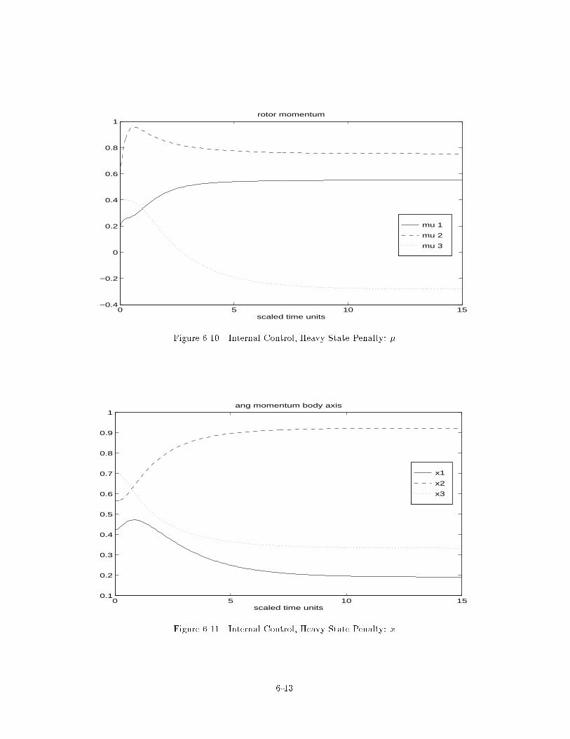
6.3.3 Simulation Results. Results for the �rst weighting set are given in Figures 6.10
through 6.15. Notice that this controller is very e�ective in reorienting the satellite. Of all the
examples presented in this thesis, this is perhaps the most promising in real application. The
controller induces a quick increase in body axis angular velocities, and then exponentially decays
them back to their rest position. Control usage is very smooth. Also remember that the dynamics
are scaled, so that the time to settle does not represent real seconds, but rather scaled time units.
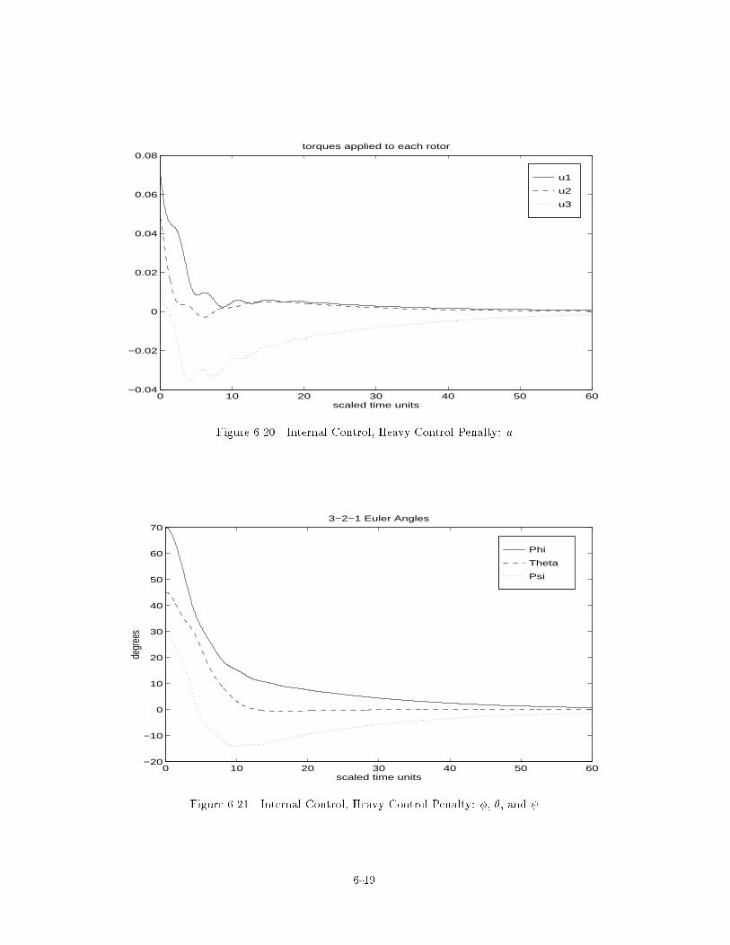
For our second example we will see how a larger control penalty impacts the problem. The
results are seen in Figures 6.16 through 6.21. This controller still provides excellent stability
properties. Now, however, instead of the sharp rise and exponential decay in angular velocities,
a sinusoidal pattern is superimposed over the growth and decay. Additionally, the settling time
has also increased. Further penalizing control usage only increases this sinusoidal nature, with a
continuing increase in time to settle.
6.4 Summary
This chapter shows that using a state dependent algebraic Riccati equation results in e�ec-
tive control usage which can be used to both stabilize and reorient a satellite. The �rst system
demonstrated the ability of NQR to command external torques to bring a satellite to rest. Since
control usage is limited by the fuel reserves of the satellite, this is not a very practical example.
This example was meant to help validate NQR as a control method.
6-12
mu 1
mu 2
mu 3
0 5 10 15−0.4
−0.2
0
0.2
0.4
0.6
0.8
1rotor momentum
scaled time units
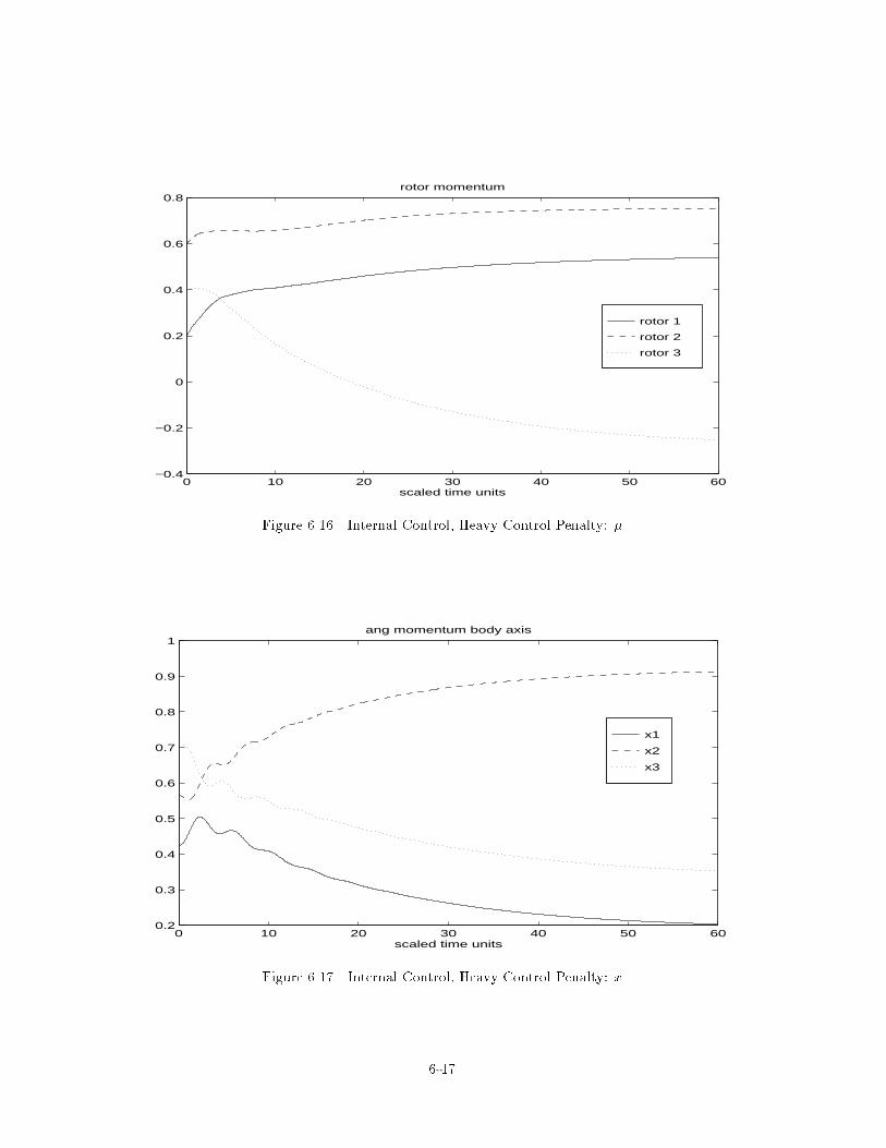
Figure 6.10 Internal Control, Heavy State Penalty: �
x1
x2
x3
0 5 10 150.1
0.2
0.3
0.4
0.5
0.6
0.7
0.8
0.9
1ang momentum body axis
scaled time units
Figure 6.11 Internal Control, Heavy State Penalty: x
6-13

w1
w2
w3
0 5 10 15−0.4
−0.35
−0.3
−0.25
−0.2
−0.15
−0.1
−0.05
0
0.05body axis ang velocities
scaled time units
Figure 6.12 Internal Control, Heavy State Penalty: !
0 5 10 15−0.2
0
0.2
0.4
0.6
0.8
1
1.2quaternions
scaled time units
Figure 6.13 Internal Control, Heavy State Penalty: q
6-14

u1
u2
u3
0 5 10 15−0.5
0
0.5
1
1.5
2torques applied to each rotor
scaled time units
Figure 6.14 Internal Control, Heavy State Penalty: u
Phi
Theta
Psi
0 5 10 15−10
0
10
20
30
40
50
60
703−2−1 Euler Angles
scaled time units
degr
ees
Figure 6.15 Internal Control, Heavy State Penalty: �, �, and
6-15
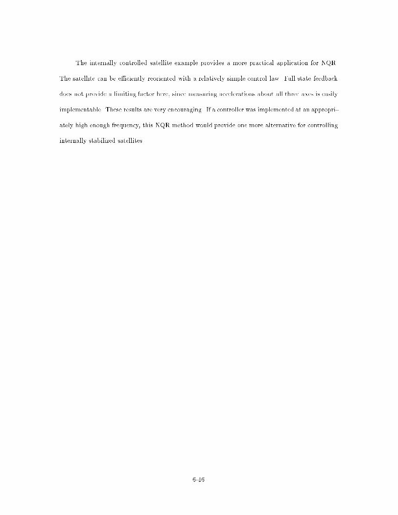
The internally controlled satellite example provides a more practical application for NQR.
The satellite can be e�ciently reoriented with a relatively simple control law. Full state feedback
does not provide a limiting factor here, since measuring accelerations about all three axes is easily
implementable. These results are very encouraging. If a controller was implemented at an appropri-
ately high enough frequency, this NQR method would provide one more alternative for controlling
internally stabilized satellites.
6-16
rotor 1
rotor 2
rotor 3
0 10 20 30 40 50 60−0.4
−0.2
0
0.2
0.4
0.6
0.8rotor momentum
scaled time units
Figure 6.16 Internal Control, Heavy Control Penalty: �
x1
x2
x3
0 10 20 30 40 50 600.2
0.3
0.4
0.5
0.6
0.7
0.8
0.9
1ang momentum body axis
scaled time units
Figure 6.17 Internal Control, Heavy Control Penalty: x
6-17
w1
w2
w3
0 10 20 30 40 50 60−0.14
−0.12
−0.1
−0.08
−0.06
−0.04
−0.02
0
0.02body axis ang velocities
scaled time units
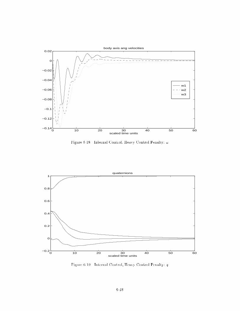
Figure 6.18 Internal Control, Heavy Control Penalty: !
0 10 20 30 40 50 60−0.2
0
0.2
0.4
0.6
0.8
1quaternions
scaled time units
Figure 6.19 Internal Control, Heavy Control Penalty: q
6-18
u1
u2
u3
0 10 20 30 40 50 60−0.04
−0.02
0
0.02
0.04
0.06
0.08torques applied to each rotor
scaled time units
Figure 6.20 Internal Control, Heavy Control Penalty: u
Phi
Theta
Psi
0 10 20 30 40 50 60−20
−10
0
10
20
30
40
50
60
703−2−1 Euler Angles
scaled time units
degr
ees
Figure 6.21 Internal Control, Heavy Control Penalty: �, �, and
6-19
VII. Arti�cial Pancreas Model
This chapter covers the modeling of human glucose and insulin dynamics as developed by
Hodel and Naylor [NHS95] of Auburn University. The model was developed in SIMULINK and
uses modules written in C. This model, the Advanced Endocrine Management of Glucose (AEMG)
model, is divided into four compartments simulating the liver, pancreas, and blood and tissue
chemistry. For further information, see the individual papers by Hodel [Hod94] and Naylor [Nay94].
The dynamics presented here consolidate the information of those four modules. No claims are made
in this thesis as to the accuracy or validity of these equations, since veri�cation is beyond the scope
of this thesis. We are merely concerned with the following problem: assuming these dynamics,
what kind of performance does a nonlinear quadratic regulator achieve?
The complexity of the AEMG model is an attempt to present a better model of glucose and
insulin dynamics. The original intent of this thesis was to investigate linear controllers for this
model. Linear controllers examined in earlier papers and in Hodel's paper were based on simpler
models and were determined to be inadequate. When this author tried to linearize the larger
AEMG model dynamics, it was determined that linearizing about equilibrium was valid for only
insigni�cant perturbations. A comparison of the linear and nonlinear dynamics in response to an
external glucose disturbance is shown in Figure 7.1. The linear response is not large enough to
warrant any control, whereas the `real' response is signi�cant and requires insulin to counter the
e�ect. This prompted the investigation into nonlinear control techniques.
7.1 Nonlinear Dynamics
The current AEMG model contains nine states given in Table 7.1, and it is highly nonlinear.
The only changes to the dynamics presented here were altering the high and low limits of some
trigger functions and the addition of a constant term in the glucose state equation. This was done
so the equations would have a steady state value equal to average normal levels in humans. The
7-1
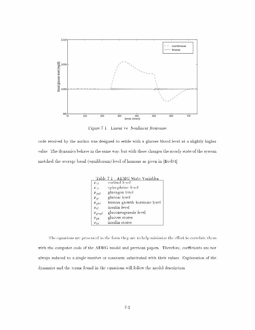
nonlinear
linear
0 10 20 30 40 50 60 7095
100
105
110
time (min)
blood
gluc
ose
level
(mg/
dl)
Figure 7.1 Linear vs. Nonlinear Response
code received by the author was designed to settle with a glucose blood level at a slightly higher
value. The dynamics behave in the same way, but with these changes the steady state of the system
matched the average basal (equilibrium) level of humans as given in [Hod94].
Table 7.1 AEMG State Variablesxcl cortisol levelxel epinephrine levelxggl glucagon levelxgl glucose levelxghl human growth hormone levelxil insulin levelxgngl gluconeogenesis levelxgs glucose storesxis insulin stores
The equations are presented in the form they are to help minimize the e�ort to correlate them
with the computer code of the AEMG model and previous papers. Therefore, coe�cients are not
always reduced to a single number or constants substituted with their values. Explanation of the
dynamics and the terms found in the equations will follow the model description.
7-2
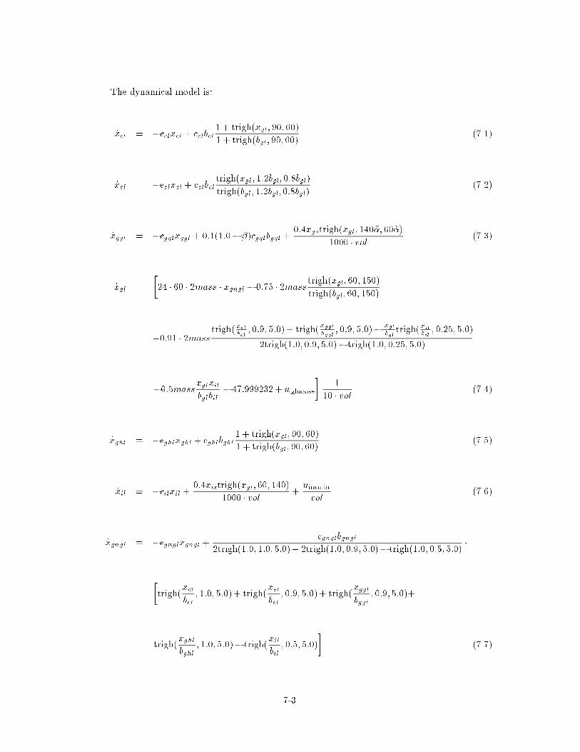
The dynamical model is:
_xcl = �cclxcl + cclbcl1 + trigh(xgl; 90; 60)
1 + trigh(bgl; 90; 60)(7.1)
_xel = �celxel + celbeltrigh(xgl; 1:2bgl; 0:8bgl)
trigh(bgl; 1:2bgl; 0:8bgl)(7.2)
_xggl = �cgglxggl + 0:1(1:0� �)cgglbggl +0:4xgstrigh(xgl; 140~�; 60~�)
1000 � vol(7.3)
_xgl =
�24 � 60 � 2mass � xgngl � 0:75 � 2mass
trigh(xgl; 60; 150)
trigh(bgl; 60; 150)
+0:91 � 2masstrigh(xel
bel; 0:9; 5:0)+ trigh(
xgglbggl
; 0:9; 5:0)�xglbgl
trigh(xilbil; 0:25; 5:0)
2trigh(1:0; 0:9; 5:0)� trigh(1:0; 0:25; 5:0)
�0:5massxglxil
bglbil� 47:999232+wglucose
�1
10 � vol(7.4)
_xghl = �cghlxghl + cghlbghl1 + trigh(xgl; 90; 60)
1 + trigh(bgl; 90; 60)(7.5)
_xil = �cilxil +0:4xistrigh(xgl; 60; 140)
1000 � vol+uinsulin
vol(7.6)
_xgngl = �cgnglxgngl +cgnglbgngl
2trigh(1:0; 1:0; 5:0)+ 2trigh(1:0; 0:9; 5:0)� trigh(1:0; 0:5; 5:0)�
�trigh(
xcl
bcl; 1:0; 5:0)+ trigh(
xel
bel; 0:9; 5:0)+ trigh(
xggl
bggl; 0:9; 5:0)+
trigh(xghl
bghl; 1:0; 5:0)� trigh(
xil
bil; 0:5; 5:0)
�(7.7)
7-3
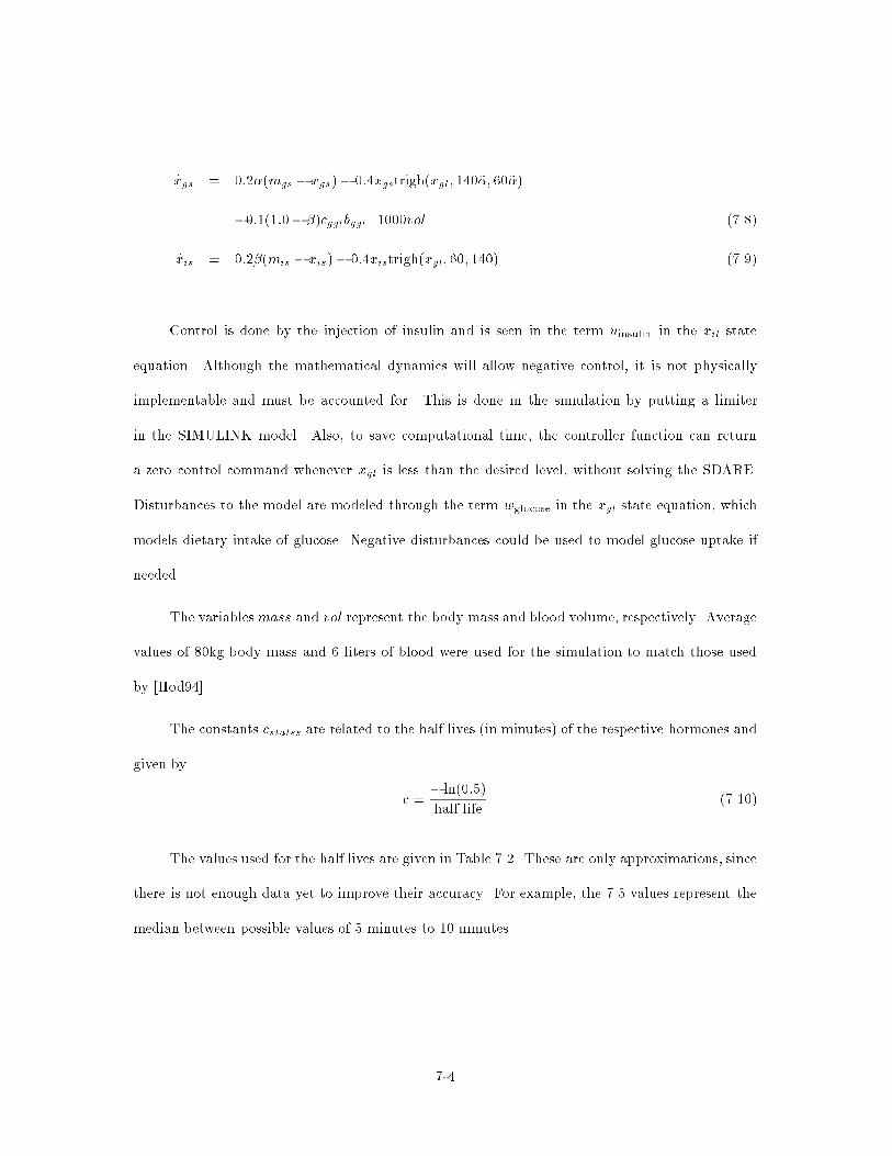
_xgs = 0:2�(mgs � xgs)� 0:4xgstrigh(xgl; 140~�; 60~�)
�0:1(1:0� �)cgglbggl � 1000vol (7.8)
_xis = 0:2�(mis � xis)� 0:4xistrigh(xgl; 60; 140) (7.9)
Control is done by the injection of insulin and is seen in the term uinsulin in the xil state
equation. Although the mathematical dynamics will allow negative control, it is not physically
implementable and must be accounted for. This is done in the simulation by putting a limiter
in the SIMULINK model. Also, to save computational time, the controller function can return
a zero control command whenever xgl is less than the desired level, without solving the SDARE.
Disturbances to the model are modeled through the term wglucose in the xgl state equation, which
models dietary intake of glucose. Negative disturbances could be used to model glucose uptake if
needed.
The variablesmass and vol represent the body mass and blood volume, respectively. Average
values of 80kg body mass and 6 liters of blood were used for the simulation to match those used
by [Hod94].
The constants cstates are related to the half lives (in minutes) of the respective hormones and
given by
c =� ln(0:5)
half life(7.10)
The values used for the half lives are given in Table 7.2. These are only approximations, since
there is not enough data yet to improve their accuracy. For example, the 7.5 values represent the
median between possible values of 5 minutes to 10 minutes.
7-4
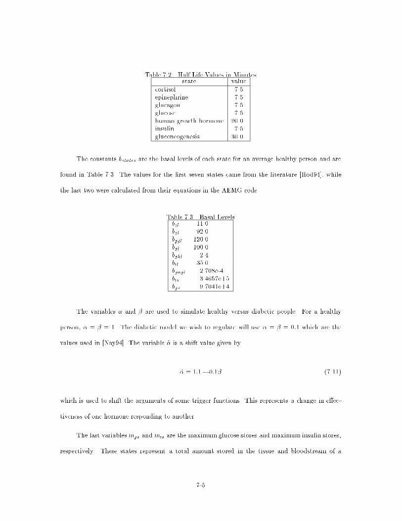
Table 7.2 Half Life Values in Minutesstate value
cortisol 7.5epinephrine 7.5glucagon 7.5glucose 7.5human growth hormone 90.0insulin 7.5gluconeogenesis 30.0
The constants bstates are the basal levels of each state for an average healthy person and are
found in Table 7.3. The values for the �rst seven states came from the literature [Hod94], while
the last two were calculated from their equations in the AEMG code.
Table 7.3 Basal Levelsbcl 11.0bel 92.0bggl 120.0bgl 100.0bghl 2.4bil 35.0bgngl 2.708e-4bis 3.4657e+5bgs 9.7041e+4
The variables � and � are used to simulate healthy versus diabetic people. For a healthy
person, � = � = 1. The diabetic model we wish to regulate will use � = � = 0:1 which are the
values used in [Nay94]. The variable ~� is a shift value given by
~� = 1:1� 0:1� (7.11)
which is used to shift the arguments of some trigger functions. This represents a change in e�ec-
tiveness of one hormone responding to another.
The last variables mgs and mis are the maximum glucose stores and maximum insulin stores,
respectively. These states represent a total amount stored in the tissue and bloodstream of a
7-5
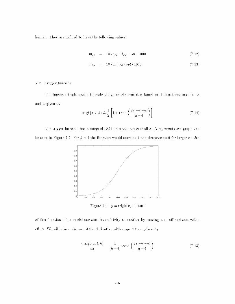
human. They are de�ned to have the following values:
mgs = 10 � cggl � bggl � vol � 1000 (7.12)
mis = 10 � cil � bil � vol � 1000 (7.13)
7.2 Trigger function
The function trigh is used to scale the gains of terms it is found in. It has three arguments
and is given by
trigh(x; l; h)d=
1
2
�1 + tanh
�2x� l � h
h� l
��(7.14)
The trigger function has a range of (0,1) for a domain over all x. A representative graph can
be seen in Figure 7.2. For h < l the function would start at 1 and decrease to 0 for larger x. Use
0 20 40 60 80 100 120 140 160 180 2000
0.1
0.2
0.3
0.4
0.5
0.6
0.7
0.8
0.9
1
Figure 7.2 y = trigh(x; 60; 140)
of this function helps model one state's sensitivity to another by causing a cuto� and saturation
e�ect. We will also make use of the derivative with respect to x, given by
dtrigh(x; l; h)
dx=
1
(h� l)sech2
�2x� l � h
h� l
�(7.15)
7-6
7.3 Control Objectives and Concerns
The purpose of examining automatic control is to eliminate the dangers diabetics face with
elevated glucose levels. Type I diabetes, or insulin-dependent diabetes mellitus, requires daily
injection of insulin to allow the body to use its glucose for energy and metabolism. The blood
glucose levels of diabetics are often elevated above normal values. Long term a�ects of this can
include vision loss, kidney failure, and neurological damage.
An automatic insulin delivery system, or arti�cial pancreas, could help reduce the long term
e�ects by providing a more natural, gradual injection of insulin based on the body's needs. One
thing to be kept in mind is that the control is strictly one way, the injection of insulin. Naturally,
this means that our controller will be ine�ective against hypoglycemia, which is when blood glucose
is at an abnormally low level. The only robustness that the arti�cial pancreas can guard against is
to make sure that the controller does not result in or send the person into hypoglycemia. However,
it is hoped that any device which is constantly monitoring blood glucose would at least provide some
warning before hypoglycemia is achieved. For further information on automatic control strategies,
see [Hod94].
We will only be simulating external disturbances of increased blood glucose to evaluate the
performance of our controllers, since the only response to a disturbance which lowers glucose, like
exercise, would be for the controller to turn o�. This e�ect is readily seen in the simulations when
glucose levels drop or are brought close to the desired level.
7.4 Control Implementation
7.4.1 Equilibrium. To use the nonlinear dynamics, we must �rst do a coordinate trans-
formation so that each transformed state settles at zero. Letting q be the equilibrium value we will
use the substitution
x = q + �x (7.16)
7-7
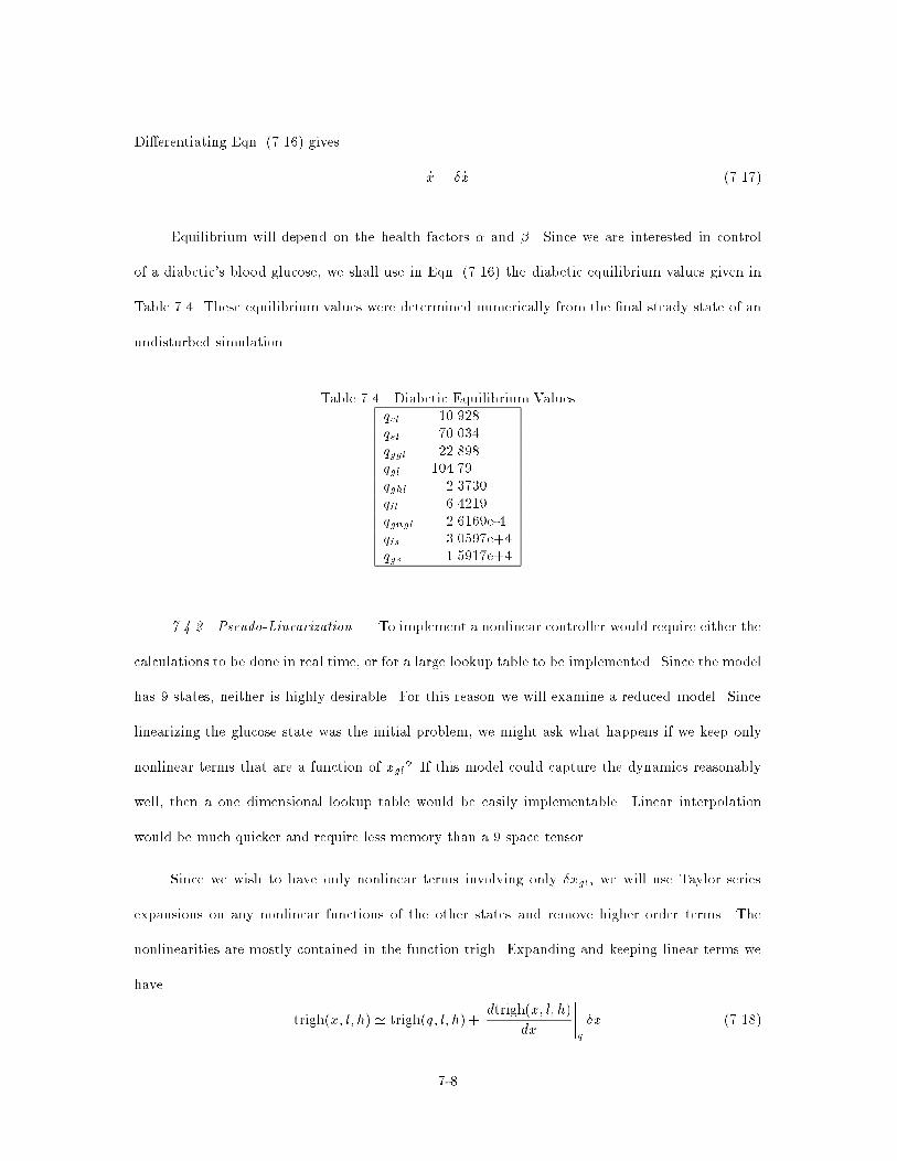
Di�erentiating Eqn. (7.16) gives
_x = � _x (7.17)
Equilibrium will depend on the health factors � and �. Since we are interested in control
of a diabetic's blood glucose, we shall use in Eqn. (7.16) the diabetic equilibrium values given in
Table 7.4. These equilibrium values were determined numerically from the �nal steady state of an
undisturbed simulation.
Table 7.4 Diabetic Equilibrium Valuesqcl 10.928qel 70.034qggl 22.898qgl 104.79qghl 2.3730qil 6.4219qgngl 2.6169e-4qis 3.0597e+4qgs 1.5917e+4
7.4.2 Pseudo-Linearization. To implement a nonlinear controller would require either the
calculations to be done in real time, or for a large lookup table to be implemented. Since the model
has 9 states, neither is highly desirable. For this reason we will examine a reduced model. Since
linearizing the glucose state was the initial problem, we might ask what happens if we keep only
nonlinear terms that are a function of xgl? If this model could capture the dynamics reasonably
well, then a one dimensional lookup table would be easily implementable. Linear interpolation
would be much quicker and require less memory than a 9 space tensor.
Since we wish to have only nonlinear terms involving only �xgl, we will use Taylor series
expansions on any nonlinear functions of the other states and remove higher order terms. The
nonlinearities are mostly contained in the function trigh. Expanding and keeping linear terms we
have
trigh(x; l; h) ' trigh(q; l; h) +dtrigh(x; l; h)
dx
����q
�x (7.18)
7-8
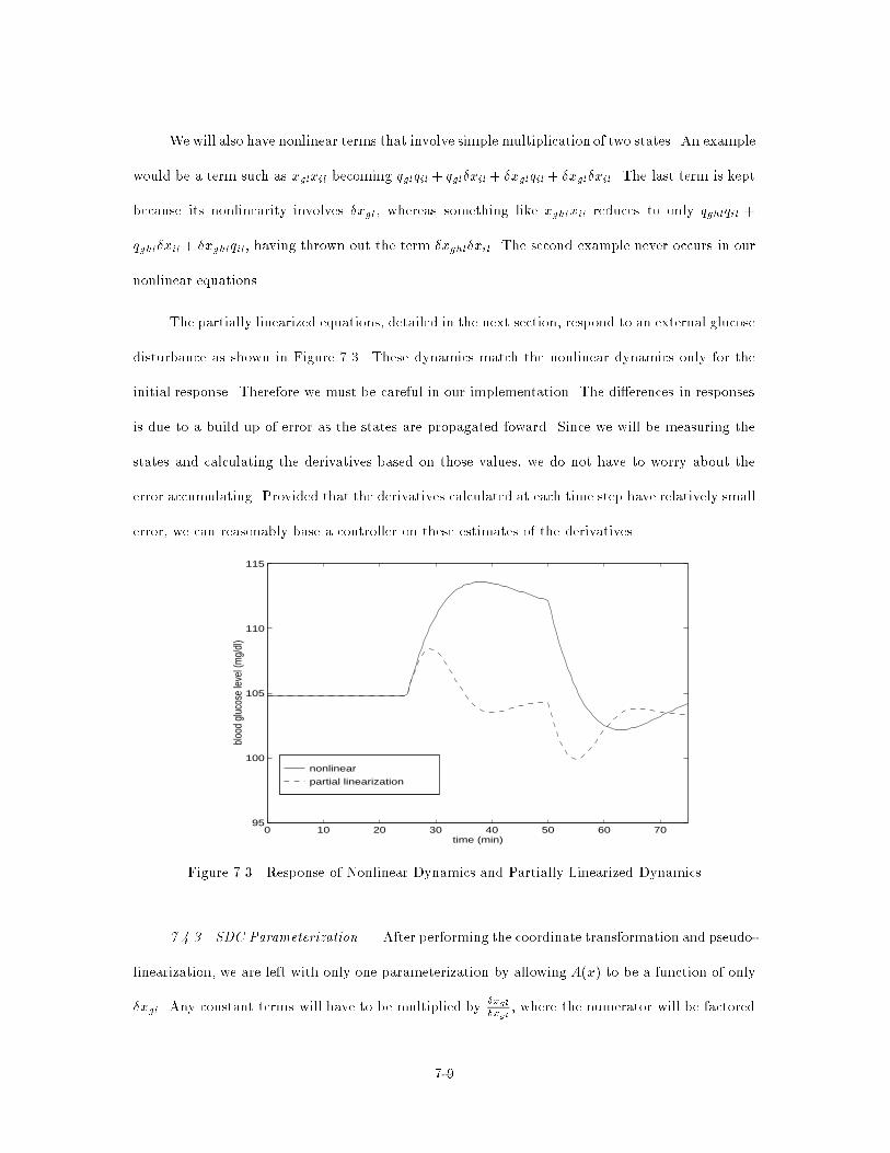
Wewill also have nonlinear terms that involve simple multiplication of two states. An example
would be a term such as xglxil becoming qglqil + qgl�xil + �xglqil + �xgl�xil. The last term is kept
because its nonlinearity involves �xgl, whereas something like xghlxil reduces to only qghlqil +
qghl�xil + �xghlqil, having thrown out the term �xghl�xil. The second example never occurs in our
nonlinear equations.
The partially linearized equations, detailed in the next section, respond to an external glucose
disturbance as shown in Figure 7.3. These dynamics match the nonlinear dynamics only for the
initial response. Therefore we must be careful in our implementation. The di�erences in responses
is due to a build up of error as the states are propagated foward. Since we will be measuring the
states and calculating the derivatives based on those values, we do not have to worry about the
error accumulating. Provided that the derivatives calculated at each time step have relatively small
error, we can reasonably base a controller on these estimates of the derivatives.
nonlinear
partial linearization
0 10 20 30 40 50 60 7095
100
105
110
115
time (min)
bloo
d gl
ucos
e le
vel (
mg/
dl)
Figure 7.3 Response of Nonlinear Dynamics and Partially Linearized Dynamics
7.4.3 SDC Parameterization. After performing the coordinate transformation and pseudo-
linearization, we are left with only one parameterization by allowing A(x) to be a function of only
�xgl. Any constant terms will have to be multiplied by�xgl�xgl
, where the numerator will be factored
7-9

out leaving the coe�cient for the �xgl state. In the following equations we will denote in bold the
�x that are factored out leaving the elements of our nonlinear matrix A(xgl). The �nal form can
be seen in Appendix A. The next chapter will detail the results of designing controllers for this
model.
Our perturbed nonlinear equations become:
� _xcl = �ccl�xcl +
��cclqcl + cclbcl
1 + trigh(qgl + �xgl; 90; 60)
1 + trigh(bgl; 90; 60)
��xgl
�xgl(7.19)
� _xel = �cel�xel +
��celqel + celbel
trigh(qgl + �xgl; 1:2bgl; 0:8bgl)
trigh(bgl; 1:2bgl; 0:8bgl)
��xgl
�xgl(7.20)
� _xggl = �cggl�xggl +
��cgglqggl + 0:1(1:0� �)cgglbggl +
0:4qgstrigh(qgl + �xgl; 140~�; 60~�)
1000 � vol
��xgl
�xgl
+0:4trigh(qgl + �xgl; 140~�; 60~�)
1000 � vol�xgs (7.21)
7-10
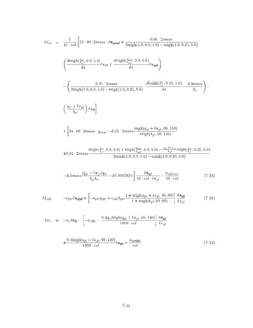
� _xgl =1
10 � vol
�24 � 60 � 2mass � �xgngl +
0:91 � 2mass
2trigh(1:0; 0:9; 5:0)� trigh(1:0; 0:25; 5:0)�
dtrigh( qel
bel; 0:9; 5:0)
dx�xel +
dtrigh(qgglbggl
; 0:9; 5:0)
dx�xggl
!
�
0:91 � 2mass
2trigh(1:0; 0:9; 5:0)� trigh(1:0; 0:25; 5:0)�dtrigh( qil
bil; 0:25; 5:0)
dx�
0:5mass
bil
!�
�qgl + �xgl
bgl
��xil
�
+
�24 � 60 � 2mass � qgngl � 0:75 � 2mass
trigh(qgl + �xgl; 60; 150)
trigh(bgl; 60; 150)
+0:91 � 2masstrigh( qel
bel; 0:9; 5:0)+ trigh(
qgglbggl
; 0:9; 5:0)�qgl+�xgl
bgltrigh( qil
bil; 0:25; 5:0)
2trigh(1:0; 0:9; 5:0)� trigh(1:0; 0:25; 5:0)
�0:5mass(qgl + �xgl)qil
bglbil� 47:999232+
��xgl
10 � vol � �xgl+wglucose
10 � vol(7.22)
� _xghl = �cghl�xghl +
��cghlqghl + cghlbghl
1 + trigh(qgl + �xgl; 90; 60)
1 + trigh(bgl; 90; 60)
��xgl
�xgl(7.23)
� _xil = �cil�xil +
��cilqil +
0:4qistrigh(qgl + �xgl; 60; 140)
1000 � vol
��xgl
�xgl
+0:4trigh(qgl + �xgl; 60; 140)
1000 � vol�xgs +
uinsulin
vol(7.24)
7-11
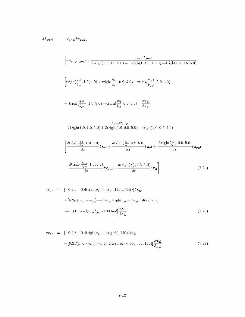
� _xgngl = �cgngl�xgngl +
��cgnglqgngl +
cgnglbgngl
2trigh(1:0; 1:0; 5:0)+ 2trigh(1:0; 0:9; 5:0)� trigh(1:0; 0:5; 5:0)�
�trigh(
qcl
bcl; 1:0; 5:0)+ trigh(
qel
bel; 0:9; 5:0)+ trigh(
qggl
bggl; 0:9; 5:0)
+ trigh(qghl
bghl; 1:0; 5:0)� trigh(
qil
bil; 0:5; 5:0)
���xgl
�xgl
+cgnglbgngl
2trigh(1:0; 1:0; 5:0)+ 2trigh(1:0; 0:9; 5:0)� trigh(1:0; 0:5; 5:0)�
"dtrigh( qcl
bcl; 1:0; 5:0)
dx�xcl +
dtrigh( qelbel; 0:9; 5:0)
dx�xel +
dtrigh(qgglbggl
; 0:9; 5:0)
dx�xggl
+dtrigh(
qghlbghl
; 1:0; 5:0)
dx�xghl �
dtrigh( qilbil; 0:5; 5:0)
dx�xil
#(7.25)
� _xgs = [�0:2�� 0:4trigh(qgl + �xgl; 140~�; 60~�)] �xgs
+ [0:2�(mgs � qgs)� 0:4qgstrigh(qgl + �xgl; 140~�; 60~�)
�0:1(1:0� �)cgglbggl � 1000vol]�xgl
�xgl(7.26)
� _xis = [�0:2� � 0:4trigh(qgl + �xgl; 60; 140)]�xis
+ [0:2�(mis � qis)� 0:4qistrigh(qgl + �xgl; 60; 140)]�xgl
�xgl(7.27)
7-12
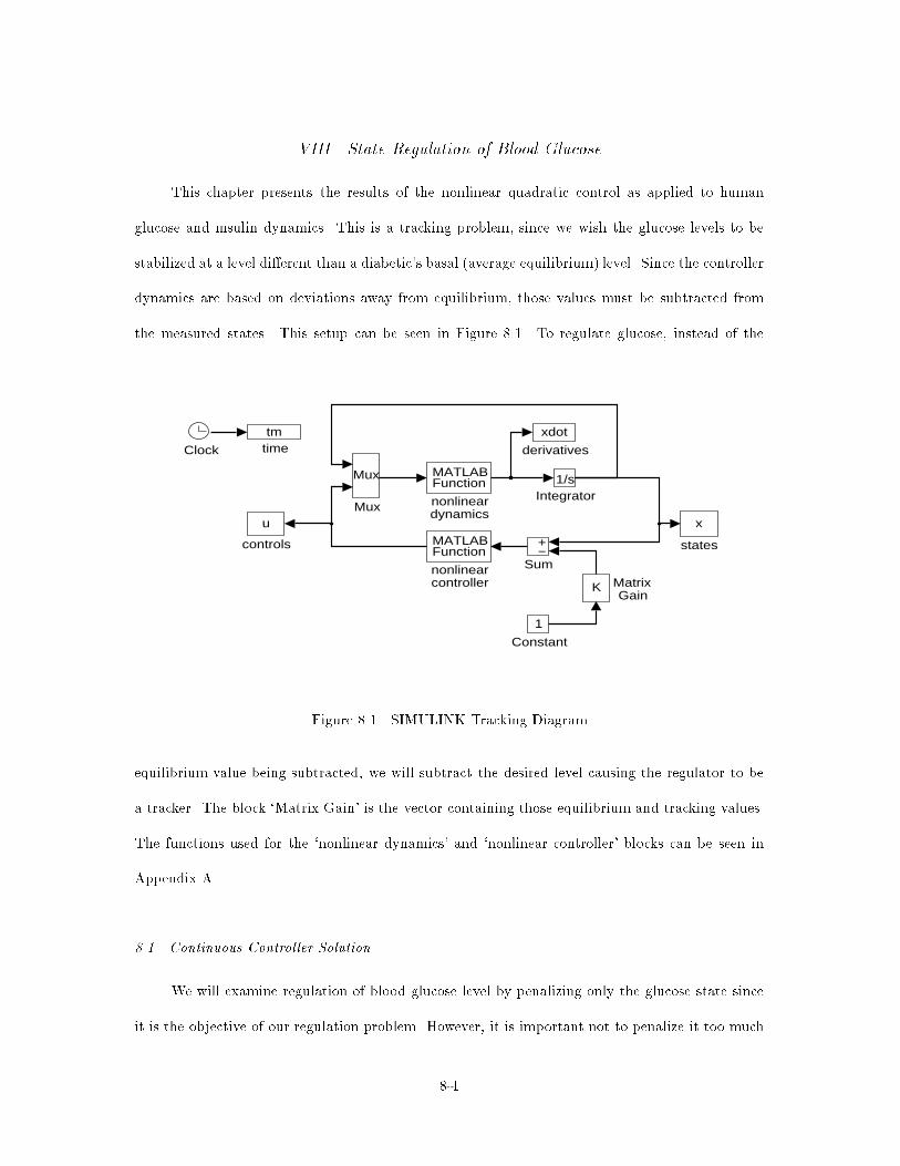
VIII. State Regulation of Blood Glucose
This chapter presents the results of the nonlinear quadratic control as applied to human
glucose and insulin dynamics. This is a tracking problem, since we wish the glucose levels to be
stabilized at a level di�erent than a diabetic's basal (average equilibrium) level. Since the controller
dynamics are based on deviations away from equilibrium, those values must be subtracted from
the measured states. This setup can be seen in Figure 8.1. To regulate glucose, instead of the
Mux
Mux
MATLABFunction
nonlinearcontroller
MATLABFunction
nonlineardynamics
1/sIntegrator
xdot
derivatives
u
controls
Clock
tmtime
+−
Sum
x
states
1
Constant
K MatrixGain
Figure 8.1 SIMULINK Tracking Diagram
equilibrium value being subtracted, we will subtract the desired level causing the regulator to be
a tracker. The block `Matrix Gain' is the vector containing those equilibrium and tracking values.
The functions used for the `nonlinear dynamics' and `nonlinear controller' blocks can be seen in
Appendix A.
8.1 Continuous Controller Solution
We will examine regulation of blood glucose level by penalizing only the glucose state since
it is the objective of our regulation problem. However, it is important not to penalize it too much
8-1
relative to insulin injection (i.e. control usage), since large doses of insulin and fast rate changes in
hormone levels are both dangerous.
We should also leave the other states unpenalized for another reason. With the injection of
insulin and change in blood glucose level, the other states will depart from their diabetic basal levels
as well. This e�ect is necessary, and we do not wish to further reduce our controller e�ectiveness
by penalizing those deviations. It might be possible to �nd a desirable level for those other states
and weight deviations from the desired levels, but this is risky and could cause a situation where
glucose will be driven below its desired value for some disturbance, resulting in hypoglycemia.
All the simulations in this section use the partially linearized equations developed in the
previous chapter. To evaluate the performance of the nonlinear quadratic regulator, we will examine
the response to a disturbance in blood glucose. The external disturbance will start at 25 minutes
and last until 50 minutes which will represent the intake of glucose from food.
To develop a feasible controller, we are �rst interested in verifying that our SDC parameter-
ization works, and that a solution to regulate glucose exists. To examine this we will �rst set up a
cheap control problem. Using as much control as is needed, we will see if the controller is e�ective.
The penalty matrices for the cheap control problem are:
Q = diag
��0 0 0 108 0 0 0 0 0
��(8.1)
R = 1 (8.2)
Figures 8.2 and 8.3 shows the cheap controller results of NQR in response to the external
glucose injection (i.e. food). The controller is indeed quite e�ective in regulating glucose level.
There is a slight steady state error because of the tracking nature of the problem, which requires
control usage as long as glucose is away from its real equilibrium. Also, there is an initial insulin
8-2
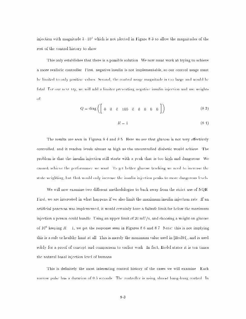
injection with magnitude 5 � 104 which is not plotted in Figure 8.3 to allow the magnitudes of the
rest of the control history to show.
This only establishes that there is a possible solution. We now must work at trying to achieve
a more realistic controller. First, negative insulin is not implementable, so our control usage must
be limited to only positive values. Second, the control usage magnitude is too large and would be
fatal. For our next try, we will add a limiter preventing negative insulin injection and use weights
of:
Q = diag
��0 0 0 100 0 0 0 0 0
��(8.3)
R = 1 (8.4)
The results are seen in Figures 8.4 and 8.5. Here we see that glucose is not very e�ectively
controlled, and it reaches levels almost as high as the uncontrolled diabetic would achieve. The
problem is that the insulin injection still starts with a peak that is too high and dangerous. We
cannot achieve the performance we want. To get better glucose tracking we need to increase the
state weighting, but that would only increase the insulin injection peaks to more dangerous levels.
We will now examine two di�erent methodologies to back away from the strict use of NQR.
First, we are interested in what happens if we also limit the maximum insulin injection rate. If an
arti�cial pancreas was implemented, it would certainly have a failsafe limit far below the maximum
injection a person could handle. Using an upper limit of 20 mU/s, and choosing a weight on glucose
of 106 keeping R = 1, we get the response seen in Figures 8.6 and 8.7. Note: this is not implying
this is a safe or healthy limit at all. This is merely the maximum value used in [Hod94], and is used
solely for a proof of concept and comparison to earlier work. In fact, Hodel states it is ten times
the natural basal injection level of humans.
This is de�nitely the most interesting control history of the cases we will examine. Each
narrow pulse has a duration of 0.5 seconds. The controller is using almost bang-bang control. In
8-3
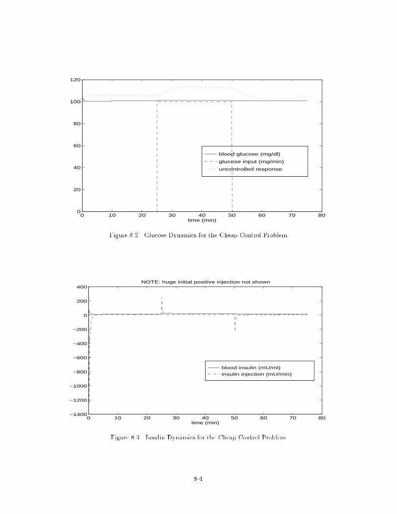
blood glucose (mg/dl)
glucose input (mg/min)
uncontrolled response
0 10 20 30 40 50 60 70 800
20
40
60
80
100
120
time (min)
Figure 8.2 Glucose Dynamics for the Cheap Control Problem
blood insulin (mU/ml)
insulin injection (mU/min)
0 10 20 30 40 50 60 70 80−1400
−1200
−1000
−800
−600
−400
−200
0
200
400
time (min)
NOTE: huge initial positive injection not shown
Figure 8.3 Insulin Dynamics for the Cheap Control Problem
8-4
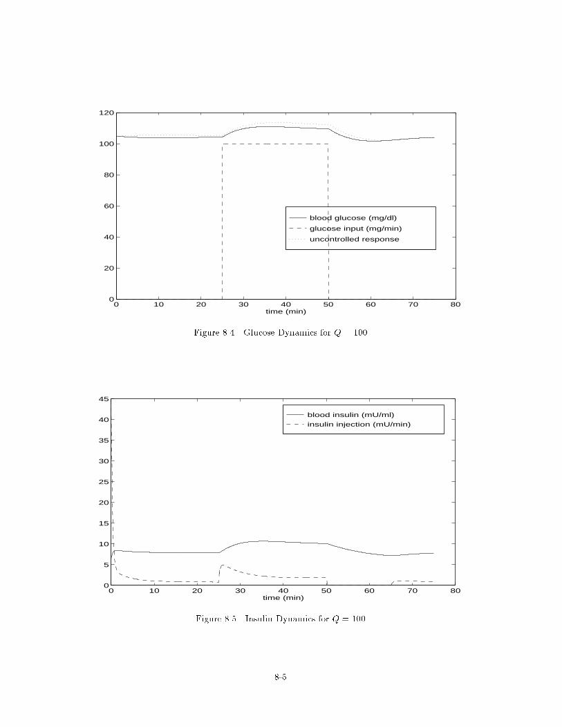
blood glucose (mg/dl)
glucose input (mg/min)
uncontrolled response
0 10 20 30 40 50 60 70 800
20
40
60
80
100
120
time (min)
Figure 8.4 Glucose Dynamics for Q = 100
blood insulin (mU/ml)
insulin injection (mU/min)
0 10 20 30 40 50 60 70 800
5
10
15
20
25
30
35
40
45
time (min)
Figure 8.5 Insulin Dynamics for Q = 100
8-5
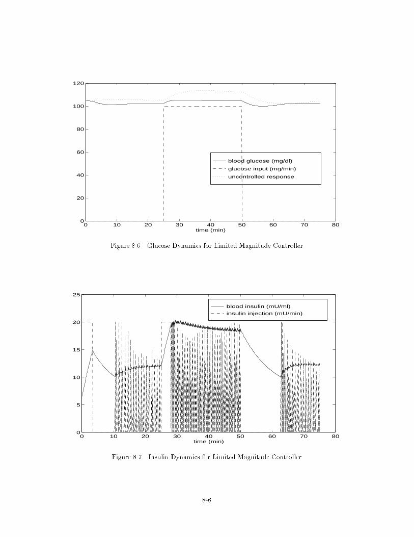
blood glucose (mg/dl)
glucose input (mg/min)
uncontrolled response
0 10 20 30 40 50 60 70 800
20
40
60
80
100
120
time (min)
Figure 8.6 Glucose Dynamics for Limited Magnitude Controller
blood insulin (mU/ml)
insulin injection (mU/min)
0 10 20 30 40 50 60 70 800
5
10
15
20
25
time (min)
Figure 8.7 Insulin Dynamics for Limited Magnitude Controller
8-6
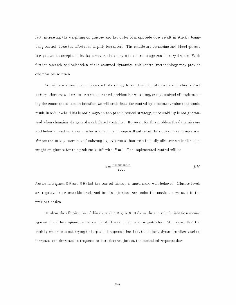
fact, increasing the weighting on glucose another order of magnitude does result in strictly bang-
bang control. Here the e�ects are slightly less severe. The results are promising and blood glucose
is regulated to acceptable levels; however, the changes in control usage can be very drastic. With
further research and validation of the assumed dynamics, this control methodology may provide
one possible solution.
We will also examine one more control strategy to see if we can establish a smoother control
history. Here we will return to a cheap control problem for weighting, except instead of implement-
ing the commanded insulin injection we will scale back the control by a constant value that would
result in safe levels. This is not always an acceptable control strategy, since stability is not guaran-
teed when changing the gain of a calculated controller. However, for this problem the dynamics are
well behaved, and we know a reduction in control usage will only slow the rates of insulin injection.
We are not in any more risk of inducing hypoglycemia than with the fully e�ective controller. The
weight on glucose for this problem is 108 with R = 1. The implemented control will be
u =ucommanded
2500(8.5)
Notice in Figures 8.8 and 8.9 that the control history is much more well behaved. Glucose levels
are regulated to reasonable levels and insulin injections are under the maximum we used in the
previous design.
To show the e�ectiveness of this controller, Figure 8.10 shows the controlled diabetic response
against a healthy response to the same disturbance. The match is quite close. We can see that the
healthy response is not trying to keep a at response, but that the natural dynamics allow gradual
increases and decreases in response to disturbances, just as the controlled response does.
8-7

blood glucose (mg/dl)
glucose input (mg/min)
uncontrolled response
0 10 20 30 40 50 60 70 800
20
40
60
80
100
120
time (min)
Figure 8.8 Glucose Dynamics for Reduced Usage Controller
blood insulin (mU/ml)
insulin injection (mU/min)
0 10 20 30 40 50 60 70 800
5
10
15
20
25
time (min)
Figure 8.9 Insulin Dynamics for Reduced Usage Controller
8-8
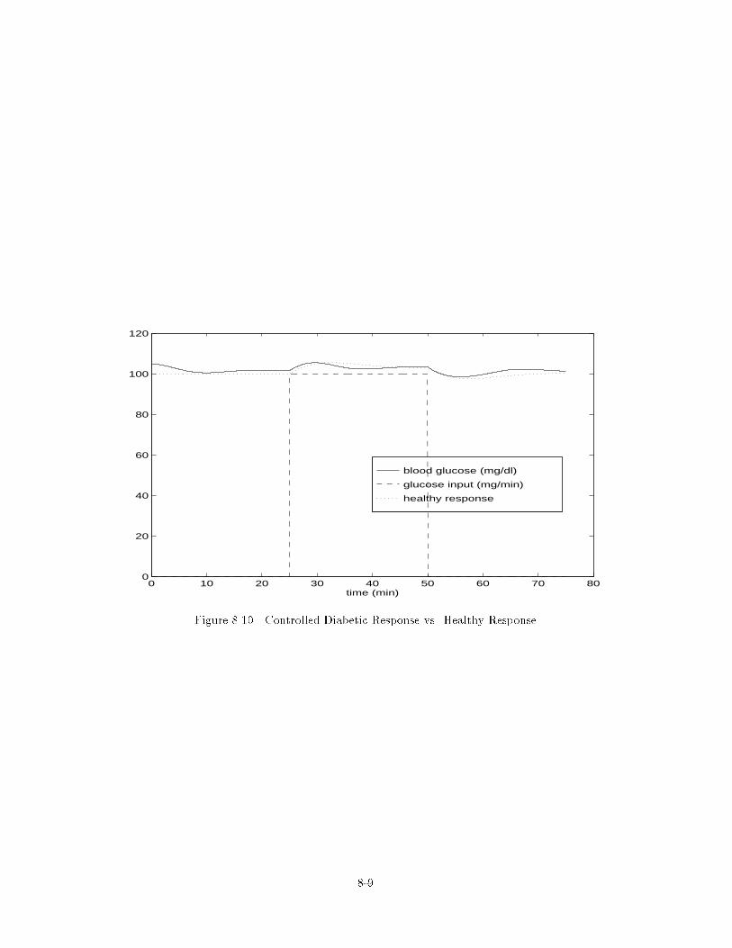
blood glucose (mg/dl)
glucose input (mg/min)
healthy response
0 10 20 30 40 50 60 70 800
20
40
60
80
100
120
time (min)
Figure 8.10 Controlled Diabetic Response vs. Healthy Response
8-9
8.2 Table Lookup Solution
The pseudo-linearization was done to form simpler calculations which could be done o�-line
and stored in a table lookup. In this section, the controller uses a gain matrix based on glucose
measurements to the nearest 0.5 mg/dl. Whereas the previous section used a continuous solution,
here the solution P is solved for a �xgl from 0.0 to 20.0 at steps of 0.5. The elements of P are then
stored as a row in a larger matrix. Instead of calculating the solution to the SDARE at each step,
�xgl is used to calculate the index to the matrix. The matrix P is reformed and used to calculate
the control usage.
The results for this methodology are given in Figures 8.11 and 8.12. The results are indistin-
guishable from the pointwise solution of above. However, the simulation ran at least twice as fast
and provides a more implementable controller. Instead of having an onboard processor to solve an
algebraic Riccati equation, an arti�cial pancreas can use the gain matrices which would be stored
in memory.
8.3 Control without Full State Feedback
Since NQR assumes full state feedback, none of the controllers examined for blood glucose
regulation are actually implementable. Presently, blood glucose is the only measurement that
would be available. Additionally, two of the states, namely glucose stores and insulin stores, are
not measurable at all. They are results of the model, and there would be no way to measure total
amounts in the body.
Perhaps the other states' in uences on control usage are relatively small compared to blood
glucose. To see if this might be reasonable, we will set the gains for all other states to 0 and
calculate the control usage. Figures 8.13 and 8.14 shows the results of this methodology. Insulin
injection achieves higher values but the deviations on blood glucose remain reasonable. Scaling
the control usage again may be e�ective in bringing the insulin injection levels back to reasonable
8-10
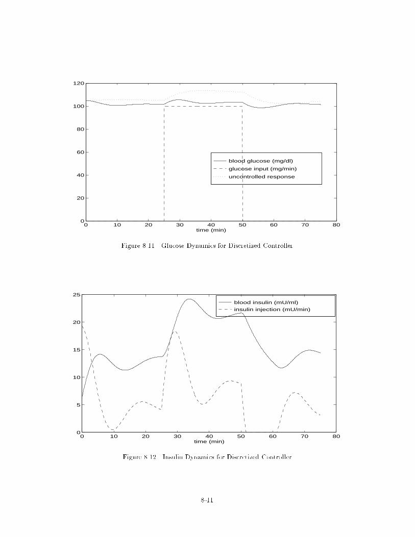
blood glucose (mg/dl)
glucose input (mg/min)
uncontrolled response
0 10 20 30 40 50 60 70 800
20
40
60
80
100
120
time (min)
Figure 8.11 Glucose Dynamics for Discretized Controller
blood insulin (mU/ml)
insulin injection (mU/min)
0 10 20 30 40 50 60 70 800
5
10
15
20
25
time (min)
Figure 8.12 Insulin Dynamics for Discretized Controller
8-11
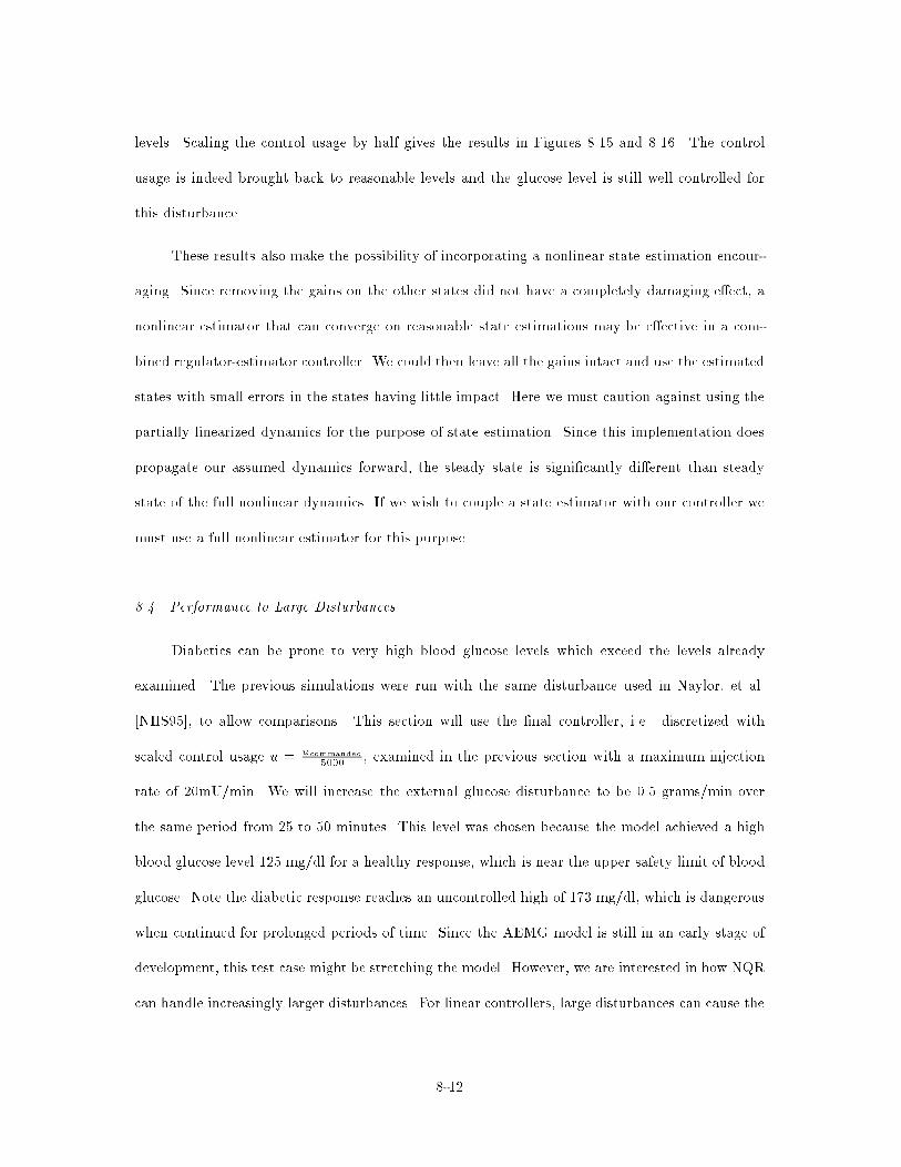
levels. Scaling the control usage by half gives the results in Figures 8.15 and 8.16. The control
usage is indeed brought back to reasonable levels and the glucose level is still well controlled for
this disturbance.
These results also make the possibility of incorporating a nonlinear state estimation encour-
aging. Since removing the gains on the other states did not have a completely damaging e�ect, a
nonlinear estimator that can converge on reasonable state estimations may be e�ective in a com-
bined regulator-estimator controller. We could then leave all the gains intact and use the estimated
states with small errors in the states having little impact. Here we must caution against using the
partially linearized dynamics for the purpose of state estimation. Since this implementation does
propagate our assumed dynamics forward, the steady state is signi�cantly di�erent than steady
state of the full nonlinear dynamics. If we wish to couple a state estimator with our controller we
must use a full nonlinear estimator for this purpose.
8.4 Performance to Large Disturbances
Diabetics can be prone to very high blood glucose levels which exceed the levels already
examined. The previous simulations were run with the same disturbance used in Naylor, et al.
[NHS95], to allow comparisons. This section will use the �nal controller, i.e. discretized with
scaled control usage u = ucommanded
5000, examined in the previous section with a maximum injection
rate of 20mU/min. We will increase the external glucose disturbance to be 0.5 grams/min over
the same period from 25 to 50 minutes. This level was chosen because the model achieved a high
blood glucose level 125 mg/dl for a healthy response, which is near the upper safety limit of blood
glucose. Note the diabetic response reaches an uncontrolled high of 173 mg/dl, which is dangerous
when continued for prolonged periods of time. Since the AEMG model is still in an early stage of
development, this test case might be stretching the model. However, we are interested in how NQR
can handle increasingly larger disturbances. For linear controllers, large disturbances can cause the
8-12
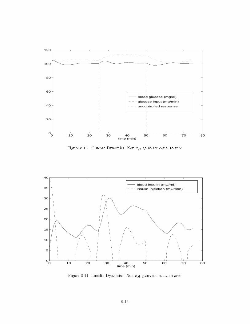
blood glucose (mg/dl)
glucose input (mg/min)
uncontrolled response
0 10 20 30 40 50 60 70 800
20
40
60
80
100
120
time (min)
Figure 8.13 Glucose Dynamics: Non xgl gains set equal to zero
blood insulin (mU/ml)
insulin injection (mU/min)
0 10 20 30 40 50 60 70 800
5
10
15
20
25
30
35
40
time (min)
Figure 8.14 Insulin Dynamics: Non xgl gains set equal to zero
8-13
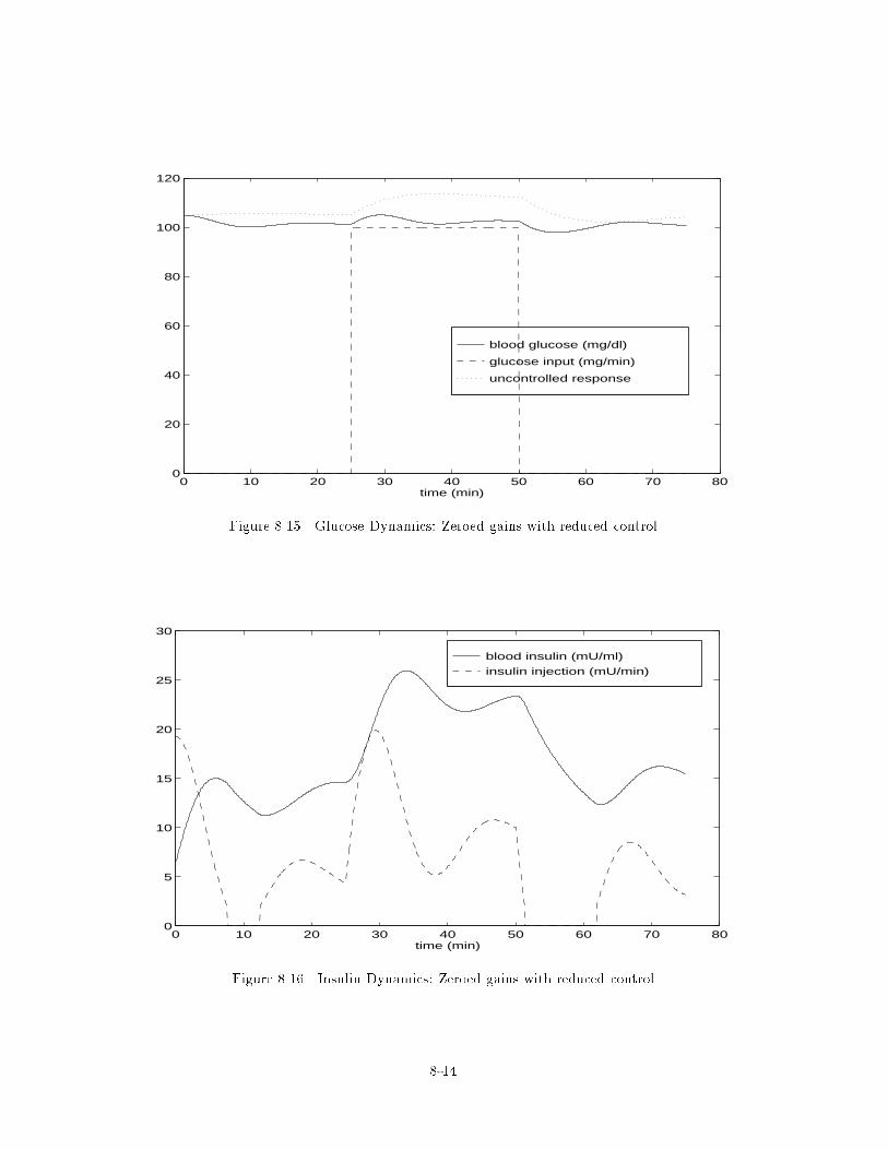
blood glucose (mg/dl)
glucose input (mg/min)
uncontrolled response
0 10 20 30 40 50 60 70 800
20
40
60
80
100
120
time (min)
Figure 8.15 Glucose Dynamics: Zeroed gains with reduced control
blood insulin (mU/ml)
insulin injection (mU/min)
0 10 20 30 40 50 60 70 800
5
10
15
20
25
30
time (min)
Figure 8.16 Insulin Dynamics: Zeroed gains with reduced control
8-14

controller to be ine�ective if the dynamics are highly nonlinear. If the NQR controller can continue
to provide encouraging results to increasingly large disturbances, then it seams reasonable that a
nonlinear quadratic regulator could provide one solution for an arti�cial pancreas.
The results are shown in Figures 8.17 and 8.18. The controlled response performs very closely
to the healthy response. This near match is of course unique for this case. For larger disturbances
the controller will result in lower performance than the average healthy performance, due to the
upper safety limit on insulin injection. Since the controller shown here is using the maximum
injection level, it will not be able to achieve a higher blood insulin level. For smaller disturbances,
the behavior approaches that seen in Figure 8.15.
Figure 8.19 shows how the controller would behave if its control usage was not limited to
a maximum value, with the corresponding control history in Figure 8.20. This shows that even
though the the control usage may not implementable, mathematically the NQR controller can keep
up with the dynamics of the nonlinear system. The overshoots increase for large disturbances, but
as a regulator NQR does return to the equilibrium values.
8.5 Summary
This chapter shows a preliminary investigation into a control methodology for an arti�cial
pancreas. While the model of human biological dynamics may be at an unvalidated stage, we
were still able to see nonlinear quadratic control e�ectively handle the assumed dynamics. Where
previous linear controllers have provided discouraging results, the SDARE calculated a suitable
controller. As the model improves, we can hope that the controller would improve as well.
On a more cautionary note, we must remind ourselves that full state feedback is not available
for this problem. Unfortunately, whereas we were able to turn o� the gains to the other states and
still achieve good results, as the model improves this may not be the case. However, these initial
8-15

controlled response
healthy response
diabetic response
0 10 20 30 40 50 60 700
20
40
60
80
100
120
140
160
180
200
time (min)
blood
gluc
ose
level
(mg/
dl)
Figure 8.17 Glucose Dynamics: 0.5 g/min disturbance
blood insulin (mU/ml)
insulin injection (mU/min)
0 10 20 30 40 50 60 70 800
5
10
15
20
25
30
35
40
45
time (min)
Figure 8.18 Insulin Dynamics: 0.5 g/min disturbance
8-16
blood glucose (mg/dl)
healthy response
0 10 20 30 40 50 60 7050
60
70
80
90
100
110
120
130
140
150
Figure 8.19 Glucose Dynamics: 0.5 g/min disturbance, no insulin cuto�
blood insulin (mU/ml)
insulin injection (mU/min)
0 10 20 30 40 50 60 700
10
20
30
40
50
60
70
80
90
100
time (min)
Figure 8.20 Insulin Dynamics: 0.5 g/min disturbance, no insulin cuto�
8-17

results should encourage us to pursue nonlinear estimation for this problem if we indeed need all
the states.
8-18
IX. Conclusions and Recommendations
9.1 Further Research Areas
This thesis provided only a �rst attempt at applying the methods of Cloutier, et al., to
practical applications. There is still further research required in each of the areas we have examined.
9.1.1 Internally Stabilized Satellites. Nonlinear quadratic regulation provided some very
encouraging results when applied to a satellite stabilized by internal momentum wheels. NQR pro-
vides both a method for stabilizing the satellite and reorienting it to any desired position. Further
research in this area should probably investigate the merits of NQR as compared to controllers
already being implemented.
Because the equations of motions were scaled, the method should be examined using real
values for the inertias. This will determine both if the torques are of reasonable magnitude, and if
the time to settle is acceptable. As the inertias represented by the scaled inertia matrix go up, the
control magnitudes and time scale likewise increase.
9.1.2 Arti�cial Pancreas Studies. This thesis only provided a proof of concept in exam-
ining the applicability of NQR as a basis for arti�cial pancreas control. While the results are quite
encouraging, there is still much more research required on the modelling side. Not only do the
biological dynamics need to be well understood, but they also require rigorous validation before
implementing a control based on them.
As the dynamic models of glucose, insulin, and related hormones improve, it is this author's
hope that a controller based on the state dependent coe�cient method of NQR will continue to be a
viable solution. It is most likely that as the equations improve, they will become only more complex
and more nonlinear, implying that nonlinear controllers may hold the most promising solutions.
Further research is not limited to the biological side. There are still many issues of NQR to be
examined, including robustness and using nonlinear estimators. There is the very real possibility
9-1
that for an improved dynamics model the gains on the other states will be signi�cant. Since NQR
is a full state feedback method, this will require it being coupled with some type of state estimator.
This could have disastrous e�ects on stability and robustness. Ultimately, since the controller would
be implemented on a human, there is no room for casual guessing.
9.1.3 Gain Scheduling Alternative. One possibility for NQR that the pancreas study
provided is the use of the state dependent coe�cient form as an alternative to gain scheduling.
Linear controllers of nonlinear systems have been adequate for many di�erent control problems
where the dynamics are reasonably represented and the perturbations relatively small. Perhaps
implementing SDC controllers on partially linearized systems will likewise be adequate for systems
with nonlinearities contained mostly in one state. This would provide a bridge between linear and
full-up nonlinear controllers. A follow up study could examine the problem where the dynamics
are represented by
_x = A(xk)x +B(xk)u (9.1)
where xk is the single state in which all nonlinearities are expressed. Perhaps there are more easily
derived optimality conditions and robustness issues for this simpler problem.
9.1.4 Discrete Implementation. What is important to remember is that the simulations
presented provided instantaneous control usage based on the values of the states. Although this
helps provide a proof of concept, it does not con�rm that we can implement the controller automat-
ically in a delayed or digitally sampled manner. Stability is provided asymptotically by providing a
pointwise stabilizing controller. If we implement the calculated control usage at any delayed time,
there is no guarantee that the commanded control will still have a stabilizing e�ect. This is of
course true for linear systems as well.
9-2

None of this should discourage one from pursuing a discrete implementation. Further research
should also look at the performance of sampling and delay in a more realistic implementation of
NQR.
9.2 Summary
While the theory of nonlinear feedback control using the state-dependent Riccati equation is
still relatively new, it appears that there may be great promise in the results. For the examples
studied in this thesis, NQR provided stabilizing controllers that were quite e�ective, and although
suboptimal still provided adequate state and control usage responses.
We have also seen nonlinear quadratic regulation used on two very di�erent dynamical sys-
tems. The method seems well suited to a variety of control problems. With further development
of the theory behind NQR, we may �nd this method to be a promising new direction in control
theory.
9-3
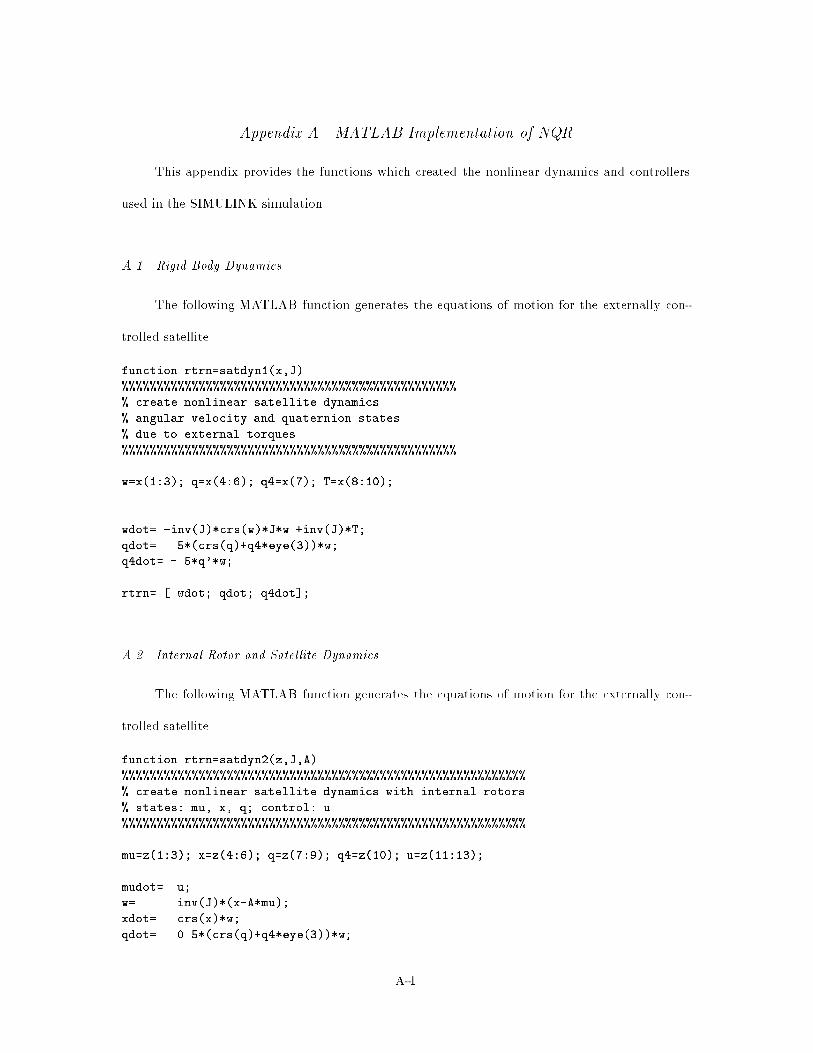
Appendix A. MATLAB Implementation of NQR
This appendix provides the functions which created the nonlinear dynamics and controllers
used in the SIMULINK simulation.
A.1 Rigid Body Dynamics
The following MATLAB function generates the equations of motion for the externally con-
trolled satellite.
function rtrn=satdyn1(x,J)
%%%%%%%%%%%%%%%%%%%%%%%%%%%%%%%%%%%%%%%%%%%%%%%%
% create nonlinear satellite dynamics
% angular velocity and quaternion states
% due to external torques
%%%%%%%%%%%%%%%%%%%%%%%%%%%%%%%%%%%%%%%%%%%%%%%%
w=x(1:3); q=x(4:6); q4=x(7); T=x(8:10);
wdot= -inv(J)*crs(w)*J*w +inv(J)*T;
qdot= .5*(crs(q)+q4*eye(3))*w;
q4dot= -.5*q'*w;
rtrn= [ wdot; qdot; q4dot];
A.2 Internal Rotor and Satellite Dynamics
The following MATLAB function generates the equations of motion for the externally con-
trolled satellite.
function rtrn=satdyn2(z,J,A)
%%%%%%%%%%%%%%%%%%%%%%%%%%%%%%%%%%%%%%%%%%%%%%%%%%%%%%%%%%
% create nonlinear satellite dynamics with internal rotors
% states: mu, x, q; control: u
%%%%%%%%%%%%%%%%%%%%%%%%%%%%%%%%%%%%%%%%%%%%%%%%%%%%%%%%%%
mu=z(1:3); x=z(4:6); q=z(7:9); q4=z(10); u=z(11:13);
mudot= u;
w= inv(J)*(x-A*mu);
xdot= crs(x)*w;
qdot= 0.5*(crs(q)+q4*eye(3))*w;
A-1
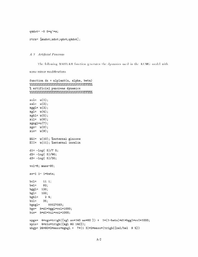
q4dot= -0.5*q'*w;
rtrn= [mudot;xdot;qdot;q4dot];
A.3 Arti�cial Pancreas
The following MATLAB function generates the dynamics used in the AEMG model with
some minor modi�cations.
function dx = nlplant(u, alpha, beta)
%%%%%%%%%%%%%%%%%%%%%%%%%%%%%%%%%%%%%
% artificial pancreas dynamics
%%%%%%%%%%%%%%%%%%%%%%%%%%%%%%%%%%%%%
xcl= u(1);
xel= u(2);
xggl= u(3);
xgl= u(4);
xghl= u(5);
xil= u(6);
xgngl=u(7);
xgs= u(8);
xis= u(9);
EGI= u(10); %external glucose
EII= u(11); %external insulin
d1= -log(.5)/7.5;
d2= -log(.5)/90;
d3= -log(.5)/30;
vol=6; mass=80;
as=1.1-.1*beta;
bcl= 11.1;
bel= 92;
bggl= 120;
bgl= 100;
bghl= 2.4;
bil= 35;
bgngl= .00027083;
bgs= 5*d1*bggl*vol*1000;
bis= 5*d1*bil*vol*1000;
upgs= .4*xgs*trigh([xgl as*140 as*60 ]) + .1*(1-beta)*d1*bggl*vol*1000;
upis= .4*xis*trigh([xgl 60 140]);
uhgp= 24*60*2*mass*xgngl + .7*(1.3)*2*mass*(trigh([xel/bel .9 5])...
A-2
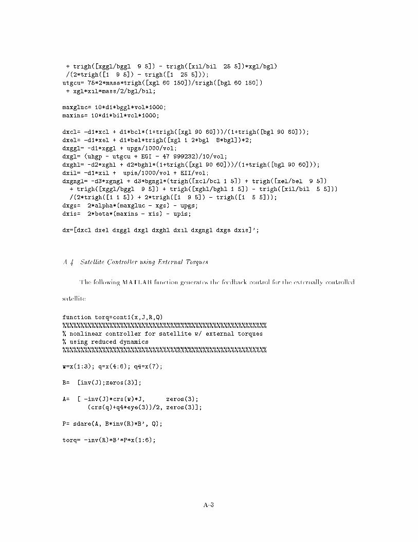
+ trigh([xggl/bggl .9 5]) - trigh([xil/bil .25 5])*xgl/bgl)...
/(2*trigh([1 .9 5]) - trigh([1 .25 5]));
utgcu=.75*2*mass*trigh([xgl 60 150])/trigh([bgl 60 150])...
+ xgl*xil*mass/2/bgl/bil;
maxgluc= 10*d1*bggl*vol*1000;
maxins= 10*d1*bil*vol*1000;
dxcl= -d1*xcl + d1*bcl*(1+trigh([xgl 90 60]))/(1+trigh([bgl 90 60]));
dxel= -d1*xel + d1*bel*trigh([xgl 1.2*bgl .8*bgl])*2;
dxggl= -d1*xggl + upgs/1000/vol;
dxgl= (uhgp - utgcu + EGI - 47.999232)/10/vol;
dxghl= -d2*xghl + d2*bghl*(1+trigh([xgl 90 60]))/(1+trigh([bgl 90 60]));
dxil= -d1*xil + upis/1000/vol + EII/vol;
dxgngl= -d3*xgngl + d3*bgngl*(trigh([xcl/bcl 1 5]) + trigh([xel/bel .9 5])...
+ trigh([xggl/bggl .9 5]) + trigh([xghl/bghl 1 5]) - trigh([xil/bil .5 5]))...
/(2*trigh([1 1 5]) + 2*trigh([1 .9 5]) - trigh([1 .5 5]));
dxgs= .2*alpha*(maxgluc - xgs) - upgs;
dxis= .2*beta*(maxins - xis) - upis;
dx=[dxcl dxel dxggl dxgl dxghl dxil dxgngl dxgs dxis]';
A.4 Satellite Controller using External Torques
The following MATLAB function generates the feedback control for the externally controlled
satellite.
function torq=cont1(x,J,R,Q)
%%%%%%%%%%%%%%%%%%%%%%%%%%%%%%%%%%%%%%%%%%%%%%%%%%%%%%%%%
% nonlinear controller for satellite w/ external torques
% using reduced dynamics
%%%%%%%%%%%%%%%%%%%%%%%%%%%%%%%%%%%%%%%%%%%%%%%%%%%%%%%%%
w=x(1:3); q=x(4:6); q4=x(7);
B= [inv(J);zeros(3)];
A= [ -inv(J)*crs(w)*J, zeros(3);...
(crs(q)+q4*eye(3))/2, zeros(3)];
P= sdare(A, B*inv(R)*B', Q);
torq= -inv(R)*B'*P*x(1:6);
A-3
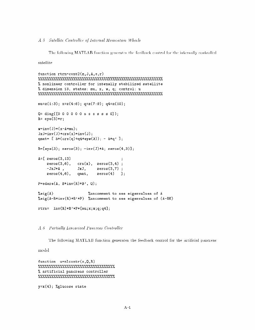
A.5 Satellite Controller of Internal Momentum Wheels
The following MATLAB function generates the feedback control for the internally controlled
satellite.
function rtrn=cont2(z,J,A,s,r)
%%%%%%%%%%%%%%%%%%%%%%%%%%%%%%%%%%%%%%%%%%%%%%%%%%%%%%%%%
% nonlinear controller for intenally stabilized satellite
% dimension 13, states: mu, x, w, q; control: u
%%%%%%%%%%%%%%%%%%%%%%%%%%%%%%%%%%%%%%%%%%%%%%%%%%%%%%%%%
mu=z(1:3); x=z(4:6); q=z(7:9); q4=z(10);
Q= diag([0 0 0 0 0 0 s s s s s s 0]);
R= eye(3)*r;
w=inv(J)*(x-A*mu);
JxJ=inv(J)*crs(x)*inv(J);
qmat= [.5*(crs(q)+q4*eye(3)); -.5*q' ];
B=[eye(3); zeros(3); -inv(J)*A; zeros(4,3)];
A=[ zeros(3,13) ;...
zeros(3,6), crs(x), zeros(3,4) ;...
-JxJ*A , JxJ, zeros(3,7) ;...
zeros(4,6), qmat, zeros(4) ];
P=sdare(A, B*inv(R)*B', Q);
%eig(A) %uncomment to see eigenvalues of A
%eig(A-B*inv(R)*B'*P) %uncomment to see eigenvalues of (A-BK)
rtrn= -inv(R)*B'*P*[mu;x;w;q;q4];
A.6 Partially Linearized Pancreas Controller
The following MATLAB function generates the feedback control for the arti�cial pancreas
model.
function u=nlcontr(x,Q,R)
%%%%%%%%%%%%%%%%%%%%%%%%%%%%%%%%%%%
% artificial pancreas controller
%%%%%%%%%%%%%%%%%%%%%%%%%%%%%%%%%%%
y=x(4); %glucose state
A-4
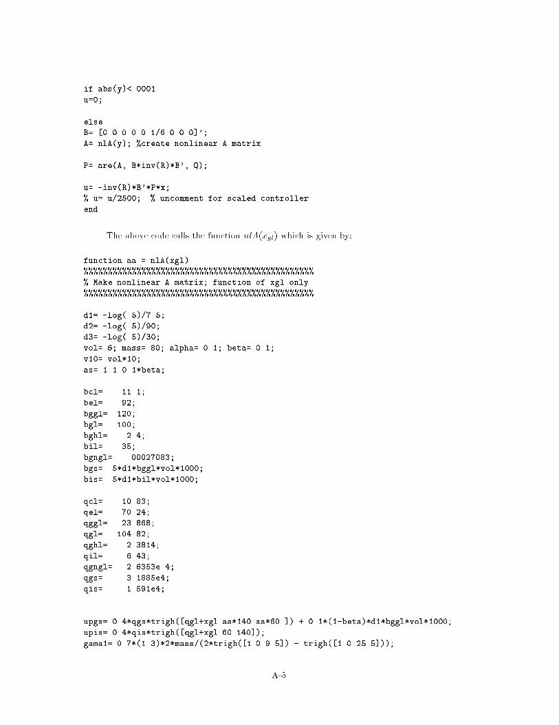
if abs(y)<.0001
u=0;
else
B= [0 0 0 0 0 1/6 0 0 0]';
A= nlA(y); %create nonlinear A matrix
P= are(A, B*inv(R)*B', Q);
u= -inv(R)*B'*P*x;
% u= u/2500; % uncomment for scaled controller
end
The above code calls the function nlA(xgl) which is given by:
function aa = nlA(xgl)
%%%%%%%%%%%%%%%%%%%%%%%%%%%%%%%%%%%%%%%%%%%%%%%%
% Make nonlinear A matrix; function of xgl only
%%%%%%%%%%%%%%%%%%%%%%%%%%%%%%%%%%%%%%%%%%%%%%%%
d1= -log(.5)/7.5;
d2= -log(.5)/90;
d3= -log(.5)/30;
vol= 6; mass= 80; alpha= 0.1; beta= 0.1;
v10= vol*10;
as= 1.1-0.1*beta;
bcl= 11.1;
bel= 92;
bggl= 120;
bgl= 100;
bghl= 2.4;
bil= 35;
bgngl= .00027083;
bgs= 5*d1*bggl*vol*1000;
bis= 5*d1*bil*vol*1000;
qcl= 10.83;
qel= 70.24;
qggl= 23.868;
qgl= 104.82;
qghl= 2.3814;
qil= 6.43;
qgngl= 2.6353e-4;
qgs= 3.1885e4;
qis= 1.591e4;
upgs= 0.4*qgs*trigh([qgl+xgl as*140 as*60 ]) + 0.1*(1-beta)*d1*bggl*vol*1000;
upis= 0.4*qis*trigh([qgl+xgl 60 140]);
gama1= 0.7*(1.3)*2*mass/(2*trigh([1 0.9 5]) - trigh([1 0.25 5]));
A-5
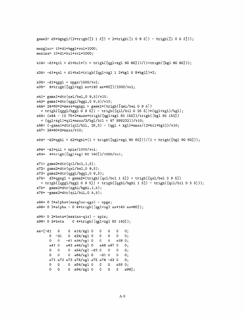
gama2= d3*bgngl/(2*trigh([1 1 5]) + 2*trigh([1 0.9 5]) - trigh([1 0.5 5]));
maxgluc= 10*d1*bggl*vol*1000;
maxins= 10*d1*bil*vol*1000;
a14= -d1*qcl + d1*bcl*(1 + trigh([qgl+xgl 90 60]))/(1+trigh([bgl 90 60]));
a24= -d1*qel + d1*bel*trigh([qgl+xgl 1.2*bgl 0.8*bgl])*2;
a34= -d1*qggl + upgs/1000/vol;
a38= .4*trigh([qgl+xgl as*140 as*60])/1000/vol;
a41= gama1*dtr(qel/bel,0.9,5)/v10;
a43= gama1*dtr(qggl/bggl,0.9,5)/v10;
a44= 24*60*2*mass*qgngl + gama1*(trigh([qel/bel 0.9 5])...
+ trigh([qggl/bggl 0.9 5]) - trigh([qil/bil 0.25 5])*(qgl+xgl)/bgl);
a44= (a44 - (0.75*2*mass*trigh([qgl+xgl 60 150])/trigh([bgl 60 150])...
+ (qgl+xgl)*qil*mass/2/bgl/bil + 47.999232))/v10;
a46= (-gama1*dtr(qil/bil,.25,5) - (qgl + xgl)*mass/(2*bil*bgl))/v10;
a47= 24*60*2*mass/v10;
a54= -d2*qghl + d2*bghl*(1 + trigh([qgl+xgl 90 60]))/(1 + trigh([bgl 90 60]));
a64= -d1*qil + upis/1000/vol;
a69= .4*trigh([qgl+xgl 60 140])/1000/vol;
a71= gama2*dtr(qcl/bcl,1,5);
a72= gama2*dtr(qel/bel,0.9,5);
a73= gama2*dtr(qggl/bggl,0.9,5);
a74= -d3*qgngl + gama2*(trigh([qcl/bcl 1 5]) + trigh([qel/bel 0.9 5])...
+ trigh([qggl/bggl 0.9 5]) + trigh([qghl/bghl 1 5]) - trigh([qil/bil 0.5 5]));
a75= gama2*dtr(qghl/bghl,1,5);
a76= -gama2*dtr(qil/bil,0.5,5);
a84= 0.2*alpha*(maxgluc-qgs) - upgs;
a88= 0.2*alpha - 0.4*trigh([qgl+xgl as*140 as*60]);
a94= 0.2*beta*(maxins-qis) - upis;
a99= 0.2*beta - 0.4*trigh([qgl+xgl 60 140]);
aa=[-d1 0 0 a14/xgl 0 0 0 0 0;...
0 -d1 0 a24/xgl 0 0 0 0 0;...
0 0 -d1 a34/xgl 0 0 0 a38 0;...
a41 0 a43 a44/xgl 0 a46 a47 0 0;...
0 0 0 a54/xgl -d2 0 0 0 0;...
0 0 0 a64/xgl 0 -d1 0 0 0;...
a71 a72 a73 a74/xgl a75 a76 -d3 0 0;...
0 0 0 a84/xgl 0 0 0 a88 0;...
0 0 0 a94/xgl 0 0 0 0 a99];
A-6
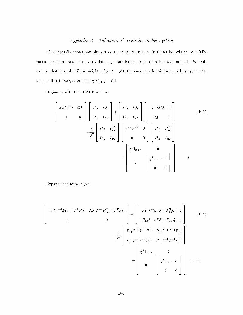
Appendix B. Reduction of Neutrally Stable System
This appendix shows how the 7 state model given in Eqn. (6.1) can be reduced to a fully
controllable form such that a standard algebraic Ricatti equation solver can be used. We will
assume that controls will be weighted by R = �2I, the angular velocities weighted by Q! = 2I,
and the �rst three quaternions by Qq1�3 = �2I
Beginning with the SDARE we have
2664 J!�J�1 QT
0 0
37752664 P11 PT
12
P12 P22
3775+
2664 P11 PT
12
P12 P22
37752664 �J�1!�J 0
Q 0
3775 (B.1)
�1
�2
2664 P11 PT
12
P12 P22
37752664 J�1J�1 0
0 0
37752664 P11 PT
12
P12 P22
3775
+
26666664
2I3�3 0
0
2664 �2I3�3 0
0 0
3775
37777775
= 0
Expand each term to get
2664 J!�J�1P11 +QTP12 J!�J�1PT
12 +QTP22
0 0
3775+
2664 �P11J
�1!�J + PT12Q 0
�P12J�1!�J + P22Q 0
3775 (B.2)
�1
�2
2664 P11J
�1J�1P11 P11J�1J�1PT
12
P12J�1J�1P11 P12J
�1J�1PT12
3775
+
26666664
2I3�3 0
0
2664 �2I3�3 0
0 0
3775
37777775
= 0
B-1
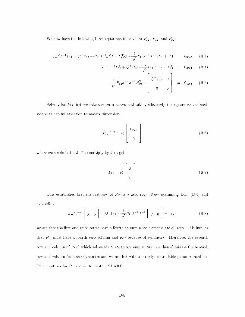
We now have the following three equations to solve for P11; P12; and P22:
J!�J�1P11 +QTP12 � P11J�1!�J + PT
12Q�1
�2P11J
�1J�1P11 + 2I = 03�3 (B.3)
J!�J�1PT12 +QTP22 �
1
�2P11J
�1J�1PT12 = 03�4 (B.4)
�1
�2P12J
�1J�1PT12 +
2664 �2I3�3 0
0 0
3775 = 04�4 (B.5)
Solving for P12 �rst we take one term across and taking e�ectively the square root of each
side with careful attention to matrix dimension
P12J�1 = ��
2664 I3�3
0
3775 (B.6)
where each side is 4� 3. Postmultiply by J to get
P12 = ��
2664 J
0
3775 (B.7)
This establishes that the last row of P12 is a zero row. Now examining Eqn. (B.4) and
expanding
J!�J�1�J 0
�+QTP22 �
1
�2P11J
�1J�1�J 0
�= 03�4 (B.8)
we see that the �rst and third terms have a fourth column whos elements are all zero. This implies
that P22 must have a fourth zero column and row because of symmetry. Therefore, the seventh
row and column of P (x) which solves the SDARE are empty. We can then eliminate the seventh
row and column from our dynamics and we are left with a strictly controllable parameterization.
The equations for P11 reduce to another SDARE.
B-2
Bibliography
CDM95. J. R. Cloutier, C. N. D'Souza, and C. P. Mracek. Nonlinear Regulation and NonlinearH1Control Via the State-Dependent Ricatti Equation Technique. Submitted for publication,1995.
Cho91. V. A. Chobotov. Spacecraft Attitude Dynamics and Control. Krieger Publishing Com-pany, 1991.
Hal95a. C. D. Hall. Asst Professor, Dept of Aero & Astro, Air Force Institute of Technology,WPAFB, OH. Personal communication, 1995.
Hal95b. C. D. Hall. Spinup Dynamics of Gyrostats. Journal of Guidance, Control, and Dynamics,18(5):1177{1183, 1995.
Hod94. A. S. Hodel. Automatic Control Issues in the Development of an Arti�cial Pancreas.Internal Auburn University Report, August 1994.
MAT. MATLAB: High performance numeric computation and visualization software. The MathWorks, Inc., Natick MA, 1994.
MCD95. C. P. Mracek, J. R. Cloutier, and C. N. D'Souza. A New Technique for NonlinearEstimation. Submitted for publication, 1995.
Nay94. J. S. Naylor. Automatic Control Issues in the Development of an Arti�cial Pancreas.Internal Auburn University Report, August 1994.
NHS95. J. S. Naylor, A. S. Hodel, and D. Schumacher. Automatic Control Issues in the Devel-opment of an Arti�cial Pancreas. In Proceedings of the American Control Conference,pages 771{775, Seattle, WA, June 1995.
ZDG95. K. Zhou, J. C. Doyle, and K. Glover. Robust and Optimal Control. Prentice Hall, 1995.
BIB-1
Vita
Captain David K. Parrish was born March 24, 1968, in Newcastle, Wyoming. He obtained his
Bachelor of Science in Aerospace Engineering from Arizona State University in May, 1991. While
awaiting active duty he substitute taught in the Scottsdale and Mesa School Districts in Arizona.
Captain Parrish started active duty in April, 1992 in the Flight Controls and Stability home o�ce
at Wright-Patterson AFB, Ohio. After six months of training, he transferred to the Training
Systems Program O�ce in Aeronautical Systems Command. Captain Parrish was responsible for
certi�cation of various simulator handling qualities, including C-141, T-1A, and the B-1B. In May
1994, Captain Parrish began his Masters Degree Program at the Air Force Institute of Technology.
Permanent address: 255 E. Warwick Ave.Newcastle, Wyoming 82701email: [email protected]
VITA-1


