Applications of Partial Differential Equations To …kazdan/japan/japan.pdfApplications of Partial...

Applications of Partial Differential Equations

To Problems in Geometry

Jerry L. Kazdan

Preliminary revised version

Copyright c© 1983, 1993 by Jerry L. Kazdan

Preface

These notes are from an intensive one week series of twenty lectures givento a mixed audience of advanced graduate students and more experiencedmathematicians in Japan in July, 1983. As a consequence, these they are notaimed at experts, and are frequently quite detailed, especially in Chapter 6where a variety of standard techniques are presented. My goal was to in-troduce geometers to some of the techniques of partial differential equations,and to introduce those working in partial differential equations to some fas-cinating applications containing many unresolved nonlinear problems arisingin geometry. My intention is that after reading these notes someone will feelthat they can cope with current research articles. In fact, the quite sketchyChapter 5 and Chapter 6 are merely intended to be advertisements to readthe complete details in the literature. When writing something like this,there is the very real danger that the only people who understand anythingare those who already know the subject. Caveat emptor .

In any case, I hope I have shown that if one assumes a few basic results onSobolev spaces and elliptic operators, then the basic techniques used in theapplications are comprehensible. Of course carrying out the details for anyspecific problem may be quite complicated—but at least the ideas should beclearly recognizable.

These notes definitely do not represent the whole subject. I did nothave time to discuss a number of beautiful applications such as minimalsurfaces, harmonic maps, global isometric embeddings (including the Weyland Minkowski problems as well as Nash’s theorem), Yang-Mills fields, thewave equation and spectrum of the Laplacian, and problems on compactmanifolds with boundary or complete non-compact manifolds. In addition,these lectures discuss only existence and uniqueness theorems, and ignoreother more qualitative problems. Although existence results seem to hold thecenter of the stage in contemporary applications, a more balanced discussionwould be important in a longer series of lectures.

The lectures assumed some acquaintance with either Riemannian geom-etry or partial differential equations. While mathematicians outside of theseareas should be able to follow these notes, it may be more difficult for themto appreciate the significance of the questions or results.

By the ruthless schedule of my charming hosts, these notes are to betyped shortly after the completion of the lectures. My hosts felt (wisely, Ithink) that it would be more useful to have an informal set of lecture notesavailable quickly rather than with longer time for a more polished manuscript.Inevitably, as befits a first draft, there will be rough edges and outright errors.I hope none of these are serious and would appreciate any corrections andsuggestions for subsequent versions.

One thing I know I would do is add a few additional sections to Chapter

i

1. In particular, there should really be some mention of Green’s functionsand at least a vague summary of the story for boundary value problems—especially the Dirichlet problem (see [N-3], pp. 41-50 for what I have inmind). Also, the dry, technical flavor of Chapter 1 should be balanced by afew more easy—but useful—applications of the linear theory. For instance,Moser’s result on volume forms [MJ-1] uses only simple Hodge theory. Butmy time deadline has come.

I hope these notes are useful to someone seeking a rapid introductionwith a minimum of background. This task is made much easier because of therecent books [Au-4] and [GT], where one can find most of the missing details.I am grateful to many Japanese mathematicians. In addition to helping makemy visit so pleasant, they are also proofreading the typed manuscript; all I’llsee is the finished product. Finally, I wish to give special thanks to ProfessorT. Ochiai for his extraordinary hospitality and thoughtfulness. I also thankthe National Science Foundation for their support.

Srinagar, India10 August 1983

Note added, June, 1993. This is an essentially unrevised version of thelectures I gave in Japan in July, 1983. The only notable addition is a sectiondiscussing the Hodge Theorem, I also took advantage of the retyping intoTEX to make a few corrections and minor clarifications in the wording. Alas,retyping introduces its own errors.

[To Do: incorporate the following into the preface]Throughout these lectures we will need some background material on

elliptic and, to a lesser extent, parabolic partial differential operators. Equa-tions that are neither elliptic nor parabolic do arise in geometry (a goodexample is the equation used by Nash to prove isometric embedding results);however many of the applications involve only elliptic or parabolic equations.For this material I have simply inserted a slightly modified version of an Ap-pendix I wrote for the book [Be-2]. This book may also be consulted forbasic formulas in geometry.2 At some places, I have added supplementaryinformation that will be used later in the lectures. I suggest that one shouldskim this chapter quickly, paying more attention to the examples than to thegeneralities, and then move directly to Chapter 6. One can refer back to theintroductory material if the need arises.

Most of our treatment is restricted to compact manifolds without bound-ary. This is simply to avoid the extra steps required to adequately discuss

2For reference, some basic geometry formulas are collected in an Appendix at the endof these notes.

ii

appropriate boundary conditions. One can also eliminate most of the com-plications in thinking about manifolds by restricting attention to the twodimensional torus with its Euclidean metric, so the Laplacian is the basicuxx + uyy , and one is considering only doubly periodic functions, say withperiod 2π . Even simpler, yet still often fruitful and non-trivial, is to reduceto the one dimensional case of functions on the circle. Here ∆u = +u′′ .This also points out one critical sign convention: for us the Laplacian hasthe sign so that ∆u = +u′′ for functions on R

1 (except that in the specialcase of the Hodge Laplacian on differential forms, we write ∆ = dd∗ + d∗das in equation (2.4) below, where in the particular case of 0 -forms this givesthe opposite sign).

To discuss the Laplacian and related elliptic differential operators, onemust introduce certain function spaces. It turns out that the spaces onethinks of first, namely C0, C1, C2 , etc. are, for better or worse, not ap-propriate; one is forced to use more complicated spaces. For instance, if∆u = f ∈ Ck , one would like to have u ∈ Ck+2 . With the exception of thespecial one dimensional case covered by the theory of ordinary differentialequations, this is false for these Ck spaces (see the example in [Mo, p. 54]),but which is true for the spaces to be introduced now. For proofs and moredetails see [F, §8-11] and [GT].

Unless stated otherwise, to be safe we will always assume that the opensets we consider are connected.

For simplicity M will always denote a C∞ connected Riemannian mani-

fold without boundary, n = dim M , and E and F are smooth vector bundles(with inner products) over M . Of course, there are related assertions if Mhas a boundary or if M is not C∞ . Sometimes we will write (Mn, g) if wewish to point out the dimension and the metric, g . The volume element iswritten dxg , or sometimes dx . By smooth we always mean C∞ ; we writeCω for the space of real analytic functions.

We also use standard multi-index notation, so if x = (x1, . . . , xn) is apoint in R

n and j = (j1, . . . , jn) is a vector of non-negative integers, then|j| = j1 + · · · + jn , xj = xj1

1 · · · xjnn , and ∂j = (∂/∂x1)

j1 · · · (∂/∂xn)jn

——————Here and below we will use the notation a(x, ∂ku) , F (x, ∂ku) , etc. to

represent any (possibly nonlinear) differential operator of order k (so here∂ku actually represents the k -jet of u ).

Last Revised: February 29, 2016

iii

iv

Contents

Preface i

1 Linear Differential Operators 11.1 Introduction . . . . . . . . . . . . . . . . . . . . . . . . . . . . . . . . . . . . 11.2 Holder Spaces . . . . . . . . . . . . . . . . . . . . . . . . . . . . . . . . . . . 61.3 Sobolev Spaces . . . . . . . . . . . . . . . . . . . . . . . . . . . . . . . . . . 71.4 Sobolev Embedding Theorem . . . . . . . . . . . . . . . . . . . . . . . . . . 81.5 Adjoint . . . . . . . . . . . . . . . . . . . . . . . . . . . . . . . . . . . . . . 101.6 Principal Symbol . . . . . . . . . . . . . . . . . . . . . . . . . . . . . . . . . 11

2 Linear Elliptic Operators 132.1 Introduction . . . . . . . . . . . . . . . . . . . . . . . . . . . . . . . . . . . . 132.2 The Definition . . . . . . . . . . . . . . . . . . . . . . . . . . . . . . . . . . 142.3 Schauder and Lp Estimates . . . . . . . . . . . . . . . . . . . . . . . . . . . 162.4 Regularity (smoothness) . . . . . . . . . . . . . . . . . . . . . . . . . . . . . 172.5 Existence . . . . . . . . . . . . . . . . . . . . . . . . . . . . . . . . . . . . . 182.6 The Maximum Principle . . . . . . . . . . . . . . . . . . . . . . . . . . . . . 212.7 Proving the Index Theorem . . . . . . . . . . . . . . . . . . . . . . . . . . . 252.8 Linear Parabolic Equations . . . . . . . . . . . . . . . . . . . . . . . . . . . 26

3 Geometric Applications 293.1 Introduction . . . . . . . . . . . . . . . . . . . . . . . . . . . . . . . . . . . . 293.2 Hodge Theory . . . . . . . . . . . . . . . . . . . . . . . . . . . . . . . . . . . 29

a) Hodge Decomposition . . . . . . . . . . . . . . . . . . . . . . . . . . . . 29b) Poincare Duality . . . . . . . . . . . . . . . . . . . . . . . . . . . . . . . 30c) The de Rham Complex . . . . . . . . . . . . . . . . . . . . . . . . . . . 31

3.3 Eigenvalues of the Laplacian . . . . . . . . . . . . . . . . . . . . . . . . . . . 323.4 Bochner Vanishing Theorems . . . . . . . . . . . . . . . . . . . . . . . . . . 36

a) One-parameter Isometry Groups . . . . . . . . . . . . . . . . . . . . . . 36b) Harmonic 1− forms . . . . . . . . . . . . . . . . . . . . . . . . . . . . . 38

3.5 The Dirac Operator . . . . . . . . . . . . . . . . . . . . . . . . . . . . . . . 393.6 The Lichnerowicz Vanishing Theorem . . . . . . . . . . . . . . . . . . . . . 403.7 A Liouville Theorem . . . . . . . . . . . . . . . . . . . . . . . . . . . . . . . 413.8 Unique Continuation . . . . . . . . . . . . . . . . . . . . . . . . . . . . . . . 43

a) The Question . . . . . . . . . . . . . . . . . . . . . . . . . . . . . . . . . 43

4 Nonlinear Elliptic Operators 454.1 Introduction . . . . . . . . . . . . . . . . . . . . . . . . . . . . . . . . . . . . 454.2 Differential Operators . . . . . . . . . . . . . . . . . . . . . . . . . . . . . . 454.3 Ellipticity . . . . . . . . . . . . . . . . . . . . . . . . . . . . . . . . . . . . . 46

v

4.4 Nonlinear Elliptic Equations: Regularity . . . . . . . . . . . . . . . . . . . . 474.5 Nonlinear Elliptic Equations: Existence . . . . . . . . . . . . . . . . . . . . 484.6 A Comparison Theorem . . . . . . . . . . . . . . . . . . . . . . . . . . . . . 504.7 Nonlinear Parabolic Equations . . . . . . . . . . . . . . . . . . . . . . . . . 524.8 A List of Techniques . . . . . . . . . . . . . . . . . . . . . . . . . . . . . . . 52

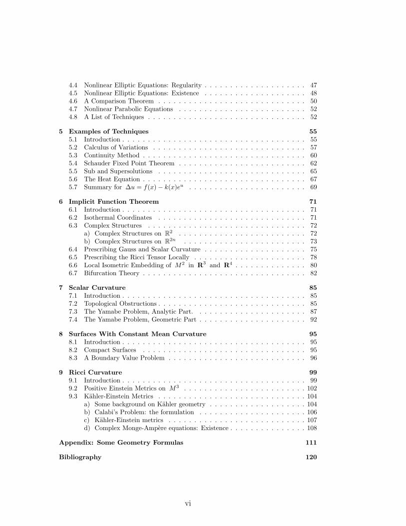
5 Examples of Techniques 555.1 Introduction . . . . . . . . . . . . . . . . . . . . . . . . . . . . . . . . . . . . 555.2 Calculus of Variations . . . . . . . . . . . . . . . . . . . . . . . . . . . . . . 575.3 Continuity Method . . . . . . . . . . . . . . . . . . . . . . . . . . . . . . . . 605.4 Schauder Fixed Point Theorem . . . . . . . . . . . . . . . . . . . . . . . . . 625.5 Sub and Supersolutions . . . . . . . . . . . . . . . . . . . . . . . . . . . . . 655.6 The Heat Equation . . . . . . . . . . . . . . . . . . . . . . . . . . . . . . . . 675.7 Summary for ∆u = f(x) − k(x)eu . . . . . . . . . . . . . . . . . . . . . . . 69

6 Implicit Function Theorem 716.1 Introduction . . . . . . . . . . . . . . . . . . . . . . . . . . . . . . . . . . . . 716.2 Isothermal Coordinates . . . . . . . . . . . . . . . . . . . . . . . . . . . . . 716.3 Complex Structures . . . . . . . . . . . . . . . . . . . . . . . . . . . . . . . 72

a) Complex Structures on R2 . . . . . . . . . . . . . . . . . . . . . . . . . 72

b) Complex Structures on R2n . . . . . . . . . . . . . . . . . . . . . . . . 73

6.4 Prescribing Gauss and Scalar Curvature . . . . . . . . . . . . . . . . . . . . 756.5 Prescribing the Ricci Tensor Locally . . . . . . . . . . . . . . . . . . . . . . 786.6 Local Isometric Embedding of M2 in R3 and R4 . . . . . . . . . . . . . . 806.7 Bifurcation Theory . . . . . . . . . . . . . . . . . . . . . . . . . . . . . . . . 82

7 Scalar Curvature 857.1 Introduction . . . . . . . . . . . . . . . . . . . . . . . . . . . . . . . . . . . . 857.2 Topological Obstructions . . . . . . . . . . . . . . . . . . . . . . . . . . . . . 857.3 The Yamabe Problem, Analytic Part. . . . . . . . . . . . . . . . . . . . . . 877.4 The Yamabe Problem, Geometric Part . . . . . . . . . . . . . . . . . . . . . 92

8 Surfaces With Constant Mean Curvature 958.1 Introduction . . . . . . . . . . . . . . . . . . . . . . . . . . . . . . . . . . . . 958.2 Compact Surfaces . . . . . . . . . . . . . . . . . . . . . . . . . . . . . . . . 958.3 A Boundary Value Problem . . . . . . . . . . . . . . . . . . . . . . . . . . . 96

9 Ricci Curvature 999.1 Introduction . . . . . . . . . . . . . . . . . . . . . . . . . . . . . . . . . . . . 999.2 Positive Einstein Metrics on M3 . . . . . . . . . . . . . . . . . . . . . . . . 1029.3 Kahler-Einstein Metrics . . . . . . . . . . . . . . . . . . . . . . . . . . . . . 104

a) Some background on Kahler geometry . . . . . . . . . . . . . . . . . . . 104b) Calabi’s Problem: the formulation . . . . . . . . . . . . . . . . . . . . . 106c) Kahler-Einstein metrics . . . . . . . . . . . . . . . . . . . . . . . . . . . 107d) Complex Monge-Ampere equations: Existence . . . . . . . . . . . . . . . 108

Appendix: Some Geometry Formulas 111

Bibliography 120

vi

vii

Chapter 1

Linear Differential Operators

1.1 Introduction

Three models from classical physics are the source of most of our knowledge of partialdifferential equations:

wave equation: uxx + uyy = utt

heat equation: uxx + uyy = ut

Laplace equation: uxx + uyy = 0.

Because the expression uxx + uyy arises so often, mathematicians generally uses theshorter notation ∆u (physicists and engineers often write ∇2u ).

One thinks of a solution u(x, y, t) of the wave equation as describing the motion of adrum head Ω at the point (x, y) at time t . We denote the boundary by ∂Ω . A typicalproblem is to specify

initial position u(x, y, 0)initial velocity ut(x, y, 0)boundary condition u(x, y, t) for (x, y) ∈ ∂Ω and t ≥ 0.

and seek the solution u(x, y, t) . Although we shall essentially not mention the waveequation again in these lectures, it is fundamental.

For the heat equation, u(x, y, t) gives the temperature at the point (x, y) at time t .Here a typical problem is to specify

initial temperature u(x, y, 0)boundary temperature u(x, y, t) for (x, y) ∈ ∂Ω and t ≥ 0

and seek u(x, y, t) for (x, y) ∈ Ω , t > 0 . This boundary condition is called a Dirichletboundary condition.

As a alternate, instead of specifying the boundary temperature, one might specifythat all or part of the boundary in insulated, so heat does not flow across the boundaryat those points. Mathematically one writes this as ∂u/∂ν = 0 , where ∂u/∂ν meansthe directional derivative in the direction ν normal to the boundary. This is called aNeumann boundary condition. Note that if one investigates heat flow on the surface of asphere or torus—or any compact manifold without boundary—then there are no boundaryconditions for the simple reason that there is no boundary.

It is clear that if a solution u(x, y, t) of the heat equation is independent of t , so oneis in equilibrium, then u is a solution of the Laplace equation (it is called a harmonic

1

2 Chapter 1. Linear Differential Operators

function). Using the heat equation model, a typical problem is the Dirichlet problem,where one specifies

boundary temperature u(x, y) = ϕ(x, y) for (x, y) ∈ ∂Ω

and one seeks the (equilibrium) temperature distribution u(x, y) for (x, y) ∈ Ω . Onemight also specify a Neumann boundary condition

∂u

∂ν= ψ(x, y)

on all or part of the boundary.From these physical models, it is intuitively plausible that in equilibrium, the max-

imum (and minimum) temperatures cannot occur at an interior point of Ω unless u ≡const., for if there were a local maximum temperature at an interior point of Ω , then theheat would flow away from that point and contradict the assumed equilibrium. This isthe maximum principle: if u satisfies the Laplace equation then

min∂Ω

u ≤ u(x, y) ≤ max∂Ω

u for (x, y) ∈ Ω.

Of course, one must give a genuine mathematical proof as a check that the model describedby the differential equation really does embody the qualitative properties predicted byphysical reasoning such as this.

For many mathematicians, a more familiar occurrence of harmonic functions is as thereal or imaginary parts of a analytic function f(z) = u + iv of one complex variable z .Indeed, one should expect that harmonic functions have many of the properties of analyticfunctions. For instance, they will automatically be smooth, and Liouville’s theorem holdsin the form: “a harmonic function defined on all of R

n that is bounded below must be aconstant.” Note that although harmonic functions do form a linear space—since they arethe kernel of a linear map—they will not have the additional special algebraic properties ofanalytic functions: closed under multiplication, inverses 1/f(z) , and under composition.These algebraic properties of analytic functions are a significant aspect of their specialnature and importance.

The inhomogeneous Laplace equation ∆u = f(x, y) is also of importance to us, par-ticularly because in these notes almost all of our discussion will concern compact manifoldswithout boundary, so there will be no boundary conditions.

In elementary courses in differential equations one main task is to find explicit formulasfor solutions of differential equations. This can only be done in the simplest situations, theresulting formulas being fundamental in more advanced work where one must gain insightwithout such explicit formulas.

example 1.1 [Laplace Equation on a Torus] We will think of the two-dimensionaltorus T 2 as the square [0, 2π]× [0, 2π] with the sides identified. Thus, smooth functionson the torus will be doubly periodic with period 2π . When can one solve the Laplaceequation

uxx + uyy = f(x, y) ? (1.1)

It is natural to use Fourier series. Thus we write f as a Fourier series and seek u as aFourier series:

f(x, y) =∑

fkℓei(kx+ℓy), u(x, y) =

∑

ukℓei(kx+ℓy).

1.1. Introduction 3

The smoothness of these functions will depend on the rate of decay of their Fourier coeffi-cients. Working formally, one substitutes u and f into the differential equation ∆u = fand matches coefficients

∑

−(k2 + ℓ2)ukℓei(kx+ℓy) =

∑

fkℓei(kx+ℓy).

For equality to hold we find that

ukℓ =−fkℓ

k2 + ℓ2(1.2)

and make the important observation that a necessary condition for a solution to exist isthat f00 = 0 , that is, from the formula for the Fourier coefficient

∫

T 2

f(x, y) dx dy = 0.

With hindsight this necessary condition was obvious by just integrating (1.1) over T 2 .From our explicit formula for the Fourier coefficients of u , this condition is also sufficient,

u(x, y) =∑ −fkℓ

k2 + ℓ2ei(kx+ℓy)

Moreover, we see that the Fourier coefficients of u decay more quickly than those of f ,so u will be smoother than f . This will be made more precise in Step 6 of Theorem3.1, where we use Sobolev spaces that will be introduced later in this chapter. After onestudies the convergence of the Fourier series, then it is easy to fully justify all of the formalcomputations we made in this example.

The solution of the Laplace equation is unique, except that one can add a constant toany solution. ¤

It is useful to remark that the identical approach to solve the wave equation formallyon the torus has immediate and serious difficulties because equation (1.2) is replaced byukℓ = −fkℓ/(k2 − ℓ2) , whose denominator is zero whenever k = ±ℓ .

example 1.2 [Heat Equation] Let (Mn, g) be a compact Riemannian manifold with-out boundary; the torus T 2 of the preceding example with the “flat” Riemannian metricg = dx2 + dy2 is a useful example. We wish to solve the heat equation

ut = ∆u for x ∈ M, (1.3)

where ∆ is the Laplace (or Laplace-Beltrami) operator of the metric g . The simplestway to define the Laplacian is to require that Green’s Theorem holds:

∫

∇u · ∇ϕdxg = −∫

(∆u)ϕdxg (1.4)

for all smooth functions ϕ with compact support. Here dxg =√

det g dx =√

|g| dx isthe Riemannian element of volume on (M, g) .

It is instructive to compute the Laplacian in local coordinates. We use functions ϕwhose support lies in a coordinate patch. Then writing gij for the inverse of the metricgij

∇u · ∇ϕ =

n∑

i,j=1

gij ∂u

∂xi

∂ϕ

∂xj


so an integration by parts gives∫

∇u · ∇ϕdxg =

∫

∑

i,j

gij ∂u

∂xi

∂ϕ

∂xj

√

|g| dx

= −∫

∑

i,j

∂

∂xi

(

gij√

|g| ∂u

∂xj

)

ϕdx

= −∫

1√

|g|∑

i,j

∂

∂xi

(

gij√

|g| ∂u

∂xj

)

ϕdxg. (1.5)

Comparing the right-hand sides of (1.4) and (1.5) we obtain the desired formula.

∆u =1

√

|g|

n∑

i,j=1

∂

∂xi

(

gij√

|g| ∂u

∂xj

)

. (1.6)

For the flat torus, gij = δij of course. Our initial condition is

u(x, 0) = f(x), (1.7)

where f is a prescribed function on M .Guided by ordinary differential equations we can write the “solution” as

u(x, t) = et∆f. (1.8)

To make sense of this we use a spectral representation of ∆ . Thus, let λj and ϕj

be the eigenvalues and corresponding eigenfunctions of −∆

−∆ϕj = λjϕj . (1.9)

For the flat torus the eigenvalues are the numbers

λkℓ = k2 + ℓ2

with corresponding orthonormal eigenfunctions

ϕkℓ =1

2πei(kx+ℓy),

where k and ℓ take all possible positive and negative integer values. Although one cancompute the eigenfunctions and eigenvalues explicitly for only a few special manifolds, bygeneral theory, it turns out that for any (M, g) the λj ’s, j = 0, 1, . . . are a discrete setof real numbers converging to ∞ . There is a corresponding complete (in L2(M) ) set oforthonormal eigenfunctions. Moreover, multiplying (1.9) by ϕj and integrating by parts(or using the divergence theorem if you prefer), we obtain

λj =

∫

|∇ϕj |2 dxg∫

ϕ2j dxg

≥ 0. (1.10)

Here the smallest eigenvalue is λ0 = 0 whose corresponding eigenfunction (normalized tohave norm 1 ) is the constant ϕ0 = 1/

√

Vol(M) .Formally, we seek a solution of (1.3) as an eigenfunction expansion

u(x, t) =∑

aj(t)ϕj(x).

1.1. Introduction 5

Substituting this into (1.3) and using the initial condition we obtain

u(x, t) =∑

j

fje−λjtϕj(x), (1.11)

where

fj =

∫

f(y)ϕj(y) dyg.

One can rewrite this solution (1.11) as

u(x, t) =

∫

H(x, y; t)f(y) dyg, (1.12)

withH(x, y; t) =

∑

j

e−λjtϕj(x)ϕj(y). (1.13)

The function H is called heat kernel or Green’s function for the problem (1.3)–(1.7). Theformulas (1.12)–(1.13) are our interpretation of (1.8), so et∆ is an integral operator (1.12)with kernel H . Then

trace et∆ =

∫

H(y, y; t) dyg =∑

j

e−λjt. (1.14)

We will use this formula in Chapter 2.7.It is difficult to extract much information from (1.12)-(1.13) unless one has more

information on the λj ’s, ϕj ’s or some formula other than (1.13) giving properties of H .These properties depend on the manifold M as well as the metric g . Nontheless, oneeasy consequence of (1.11) and (1.12) is a simple formula for the equilibrium temperature:

limt→∞

u(x, t) = average of f =1

Vol(M)

∫

f dx. (1.15)

To prove this, one notes from (1.10) that λ0 = 0 , λj > 0 for j ≥ 1 and, as pointed out

above, ϕ0(x) = constant = Vol(M)−12 . Then by (1.13)

limt→∞

H(x, y, t) = Vol (M)−1

so the assertion now follows from (1.12). The formula (1.15) states that the equilibriumtemperature is the average of the initial temperature—which is amusing but hardly sur-prising. ¤

example 1.3 [Laplace Equation on a Compact Manifold] We can apply themethod of the previous example to extend the first example to solve the Laplace equation

∆u = f

on an arbitrary compact connected manifold ( M, g ) without boundary. As a preliminarystep, we observe that the only solution of the homogeneous equation is u = const. . Thisfollows by multiplying the equation by u and then integrating by parts:

0 =

∫

M

u∆u dxg = −∫

M

|∇u|2 dxg


Thus ∇u = 0 so u is a constant. If we simply integrate ∆u = f over M , then by thedivergence theorem just as on the torus we obtain the necessary condition for solvability

0 =

∫

M

∆u dxg =

∫

M

f dxg

To find a formula for a solution we simply replace the use of Fourier series in ourdiscussion of the torus T 2 by the eigenvalues and eigenfunctions of the Laplacian. Thus,we write

f(x) =∑

fkϕk(x) and we seek u(x) =∑

ukϕk(x),

where, since the ϕk are orthonormal, in the L2 inner product we have

fk = 〈f, ϕk〉 and uk = 〈u, ϕk〉.

Substituting in the Laplace equation gives

uk = − fk

λk.

Just as in the case of the torus, because λ0 = 0 we again are led to the necessarycondition 〈f, ϕ0〉 = 0 for solvability. Because ϕ0 is a constant, this means that f mustbe orthogonal to the constants. We can formally write the solution as,

u(x) = −∑ 〈f, ϕk〉

λkϕ(x).

It is sometimes convenient to rewrite this in the form

u(x) =

∫

M

G(x, y)f(y) dyg (1.16)

where we have introduced Green’s function or Green’s kernel

G(x, y) = −∑ ϕk(x)ϕk(y)

λk

Conceptually, the advantage of formula (1.16) is that it shows that we should think ofthis integral operator as the “inverse” of the Laplacian. We must be careful in using theword “inverse” here since there is the necessary condition that f be orthogonal to theconstants, and also that the solution u is only unique up to an additive constant. ¤

Many are dismayed when the solutions of differential equations are presented, as wedid in both of our examples, by infinite series. Infinite series are more often thought ofas questions than as answers. Yet these infinite series have already yielded some usefulinformation and concepts. They also indicate directions of thought toward proving relatedresults using procedures that do not involve infinite series. The goal of computations is notformulas, it is not numbers. It is insight and understanding. Over the past two centuriesthe above infinite series have greatly enriched us.

1.2 Holder Spaces

From calculus one knows that

regularity: if u′′ = f ∈ Ck then u ∈ Ck+2

existence: if f ∈ Ck then there is a u ∈ Ck+2 with u′′ = f.

1.3. Sobolev Spaces 7

Thus, one might anticipate that, at least locally,

if ∆u = f ∈ Ck then u ∈ Ck+2

given any f ∈ Ck there is some u ∈ Ck+2 such that ∆u = f.

Each of these last two assertions is false except in dimension one (see the example in[Mo, p. 54]). But they are almost true. The trouble is that the spaces Ck are not reallyappropriate. After a century we have learned to use the Holder spaces Ck, α , where0 < α < 1 , and Sobolev spaces Hp,k , 1 < p < ∞ (here the p is as in the Lebesguespaces Lp ). If in the above assertions one replaces Ck and Ck+2 by Ck, α and Ck+2,α

(or by Hp,k and Hp, k+2 ), then they become true.With this as motivation, we define the Holder spaces in this section and Sobolev spaces

in the next section.Let A ⊂ R

n be the closure of a connected bounded open set and 0 < α < 1 . Thenf : A → R is Holder continuous with exponent α if the following expression is finite

[f ]α,A = supx,y∈Ax6=y

|f(x) − f(y)||x − y|α . (1.17)

The simplest example of such a function is f(x) = |x|α in a bounded set containing theorigin. Let Ω ⊂ R

n be a connected bounded open set. The Holder space Ck, α(Ω) isthe Banach space of real valued functions f defined on Ω all of whose kth order partialderivatives are Holder continuous with exponent α . The norm is

|f |k+α = ‖f‖Ck(Ω) + max|j|=k

[∂jf ]α,Ω, (1.18)

where ‖ ‖Ck(Ω) is the usual Ck norm. On a manifold, M , one obtains the space

Ck, β(M) by using a partition of unity. Note that if 0 < α < β < 1 , then Ck, β(M) →Ck, α(M) and by the Arzela—Ascoli theorem, this embedding is compact [For Banachspaces A , B , a continuous map T : A → B is compact if for any bounded set Q ⊂ A ,the closure of its image T (Q) is compact. Equivalently, for every bounded sequencexj ∈ A there is a subsequence xjk

so that T (xjk) converges to a point in B .]

The Holder space for α = 1 is just the space of Lipschitz continuous functions. Theydo not (yet) fit into the theory; see [FK] for more recent information.1

1.3 Sobolev Spaces

For f ∈ C∞(M), 1 ≤ p < ∞ , and an integer k ≥ 0 define the norm

‖f‖k,p =

[∫

M

∑

0≤|j|≤k

|Djf |p dxg

]1/p

, (1.19)

where |Djf | is the pointwise norm of the j -th covariant derivative. The Sobolev spaceHp,k(M) is the completion of C∞(M) in this norm; equivalently, by using local co-ordinates and a partition of unity, one can describe Hp,k(M) as equivalence classes ofmeasurable functions all of whose partial derivatives up to order k are in Lp(M) . Thespace Hp,k(M) is a Banach space, and is reflexive if 1 < p < ∞ . If p = 2 these spaces

1As an exercise, show that if a function is Holder continuous for some α > 1 , then itmust be a constant.


are Hilbert spaces with the obvious inner products. This simplest case, p = 2 , is generallyadequate for linear problems (such as Hodge theory); nonlinear problems make frequentuse of arbitrary values of p . The alternate notation Hp,k , Lp

k , and W pk are often used

instead of Hp,k . For a vector bundle E with an inner product one defines Hp,k(E)similarly.2

Note that if (within the same differentiable structure) one changes the metric on acompact Riemannian manifold (M, g) , then the norms and inner products on the spacesCk, α(M) and Hp,k(M) do change; however the new norms are equivalent to the old onesso the topologies do not change.

1.4 Sobolev Embedding Theorem

It is important to investigate relationships among these spaces Ck, α and Hp,k and also tothe familiar spaces Ck(Ω) . For instance, as we shall see shortly, there is a psychologicallyreassuring fact that if f ∈ Hp,k for all k , then f ∈ C∞ .

The essence of this study are inequalities relating the various norms. The inequalitiesare called Sobolev inequalities. This is quite simple if Ω is the interval Ω = 0 < x < cin R

1 . For convenience, say c ≥ 1 . Then

u(x) = u(y) +

∫ x

y

u′(t) dt ≤ |u(y)| +∫ c

0

|u′(t)|dt

so, integrating this with respect to y we obtain (using c ≥ 1 )

|u(x)| ≤∫ c

0

(|u′(t)| + |u(t)|) dt. (1.20)

Using Holder’s inequality for the Lp version, one can rewrite the above as

‖u‖C0 ≤ ‖u‖H1,1 ≤ c1/r‖u‖Hp,1 for any p ≥ 1, and 1p + 1

r = 1.

Thus, a Cauchy sequence in Hp,1 is also Cauchy in C0 , so we have a continuous embed-ding of Hp,1 → C0 . Observe that if, say, u(0) = 0 , then we can let y = 0 in the firststep above and obtain

|u(x)| ≤∫ c

0

|u′(t)| dt. (1.21)

In this case it is particularly clear that the Sobolev inequalities are just generalizations onthe mean value theorem, since they show how one can estimate a function in terms of itsderivatives. As an exercise, it is interesting to show that (1.21) also holds if one replacesthe assumption u(0) = 0 with

∫ c

0u = 0 . In general one needs a term involving |u| in

(1.20) since otherwise one could add a constant to u and increase the left side but notthe right.

In higher dimensions, Ω ⊂ Rn , the story is similar but more complicated. The result

is called the Sobolev embedding theorem.First we give a few easy but useful observations. One is that if f ∈ C0(M) and if we

write‖f‖∞ = max

x∈M|f(x)|

2While we write C∞(M) for smooth real (or complex) valued functions on M , byC∞(E) we mean smooth sections of a vector bundle E .

1.4. Sobolev Embedding Theorem 9

thenlim

p→∞‖f‖Lp(M) = ‖f‖∞ (1.22)

Proof: Given ǫ > 0 , let Mǫ = x ∈ M : |f(x)| ≥ ‖f‖∞ − ǫ . Then

(‖f‖∞ − ǫ)Vol(Mǫ)1/p ≤ ‖f‖Lp(M) ≤ ‖f‖∞ Vol(M)1/p.

Now let p → ∞ .Another elementary inequality—an immediate consequence of Holder’s inequality ap-

plied to f = 1 · f —states that if 1 ≤ q ≤ p , then

‖f‖Lq(M) ≤ Vol(M)(p−q)/pq‖f‖Lp(M). (1.23)

This shows that if both ℓ ≤ k and r ≤ p , then there is a continuous injection Hp,k(M) →Hq,ℓ(M) . We used this above with k = ℓ = 1 to obtain the Lp version of (1.20) fromthe L1 version.The Sobolev Embedding Theorem gives many other such relationships.Among other things, they generalize the mean value theorem in that they give estimatesfor various norms of a function in terms of norms of its derivatives. Recall that n = dimMand let δ(p, k) = k − n

p .

Theorem 1.1 [Sobolev Inequalities and Embedding Theorem]. Let 0 ≤ ℓ ≤k be integers and assume f ∈ Hp,k(M) .(a) If δ(p, k) < ℓ (that is, k − ℓ < n/p ) and if q satisfies

δ(q, ℓ) ≤ δ(p, k), equivalently,1

p− k − ℓ

n≤ 1

q, (1.24)

then there is a constant c > 0 independent of f such that

‖f‖ℓ,q ≤ c‖f‖k,p. (1.25)

Thus there is a continuous inclusion Hp,k(M) → Hq,ℓ(M) . Moreover, if ℓ < k andstrict inequality holds in (1.24), then this inclusion is a compact operator.(b) If ℓ < δ(p, k) < ℓ + 1 (that is, k − ℓ − 1 < n/p < k − ℓ ), let α = δ(p, k) − ℓ so0 < α < 1 . Then there is a constant c independent of f such that

‖f‖δ(p,k) = ‖f‖ℓ+α ≤ c‖f‖k,p. (1.26)

Thus, there is a continuous inclusion Hp,k(M) → Cδ(p,k) = Ck−np (M) = Cℓ+α(M) and

a compact inclusion Hp,k(M) → Cγ(M) for 0 < γ < δ(p, k) .

For the inclusion Hp,k(M) → Cℓ, α we naturally identify functions that differ only onsets of measure zero. The compactness assertions of part (a) in this theorem were provedby Rellich for p = 2 and generalized by Kondrachov. Note that all of the above results areproved first for a smoothly bounded open set in R

n and then extended to vector bundlesover compact manifolds using a partition of unity.

Some useful special cases (or easy consequences) of the theorem are:

(i) if f ∈ Hp,k(M) and p > n , then f ∈ Ck−1(M) ,

(ii) the inclusion Hp,k+1(M) → Hp,k(M) is compact,

(iii) if f ∈ Hp,k(M) and pk > n , then f ∈ C0(M) ,

(iv) C∞ = ∩k Hp,k for any 1 < p < ∞ ,


(v) if f ∈ H2,1(M) , then f ∈ L2n/(n−2)(M) (here n ≥ 3) , and there are constantsA , B > 0 independent of f such that

‖f‖L2n/(n−2) ≤ A‖Df‖L2 + B‖f‖L2 . (1.27)

The value q = 2n/(n − 2) in (1.27) is the largest number for which (1.25) holds in thecase k = 1 , p = 2 . It is a “limiting case” of the Sobolev inequality. The smallest valueof A for which there is some constant B such that (1.27 holds is known (see [GT; p. 151]and also [Au-4]). This smallest constant is independent of the manifold M . On the otherhand, for fixed B > 0 the smallest permissible value of A does depend on the geometryof M and is related to the isoperimetric inequality (see [Gal]), [SalC]. Related inequalitiesfor limiting cases have been found [T-1], [BW], [Au-2], [L], and play an important role inseveral recent geometric problems.

Since the condition (1.24) and the related condition in part b) may seem mysterious,it may be useful to point out that they are both optimal and easy to discover by using“dimensional analysis”. Because this technique is not as widely known as it should be,we illustrate it for example with ℓ = 0 in (1.24). Let ϕ ∈ C∞

c (|x| < 1) , ϕ 6≡ 0 , and letfλ(x) = ϕ(λx) ∈ C∞

c (|x| < 1) for λ ≥ 1 . Applying (1.25) with ℓ = 0 to the fλ anddoing a brief computation, one obtains

‖ϕ‖Lq ≤ cλk+n(

1q − 1

p )‖ϕ‖k,p.

Letting λ → ∞ there is a contradiction unless (1.24) holds. This example uses the con-formal map x 7→ λx ; it leads one to suspect that conformal deformations of metrics leadone to the limiting case of the Sobolev inequality. This suspicion is verified in Chapter 5.1.

There is a separate collection of related theorems, called trace theorems, concerning therestrictions of functions in Sobolev spaces to submanifolds. This is particularly importantfor boundary value problems since the boundary is usually a submanifold of some sort. Atypical result is that if Γ ⊂ Ω is a smooth hypersurface, then for k > 1/2 the restriction

operator γ : H2,k(Ω) → H2,s− 12 (Γ) is a continuous map onto all of H2,k− 1

2 . To makesense of this, one needs to define Sobolev spaces Hp,k (and related Besov spaces) wherek is not necessarily an integer. Since we will not need these results, we forgo furtherdiscussion (see [Ad]).

1.5 Adjoint

History sometimes takes a surprising path. Before matrices were even defined the adjointof a differential operator was introduced by Lagrange (the Lagrange identity for ordi-nary differential equations); moreover, Green proved the self-adjointness of the Laplacian(Green’s second identity). On R

1 with the L2 inner product, the adjoint of D = d/dxis found simply by integrating by parts: for all ϕ , ψ ∈ C∞

c (i.e. compact support)

〈ϕ, Dψ〉 =

∫

ϕψ′ dx = −∫

ϕ′ψ dx = 〈−Dϕ, ψ〉.

Thus, the adjoint of d/dx is −d/dx . More correctly, because d/dx is an unboundedoperator on L2 and thus not defined on the whole Hilbert space, this is the formaladjoint. The strict Hilbert space adjoint requires additional attention to the domain ofdefinition of the operator . We used smooth functions with compact support to avoidissues concerning the boundary and smoothness.

1.6. Principal Symbol 11

The usual rules hold for the adjoint of a sum and the adjoint of a product: (L+M)∗ =L∗ + M∗ and (LM)∗ = M∗L∗ . The second derivative operator D2 is thus formally self-adjoint.

Similarly, if E and F are smooth Hermitian vector bundles over M and if P :C∞(E) → C∞(F ) is a linear differential operator, then one can use the L2 inner productto define the formal adjoint, P ∗ , by the usual rule

〈Pu, v〉F = 〈u, P ∗v〉E

for all smooth sections u ∈ C∞(E)c , and v ∈ C∞(F )c . Since the supports of u and vcan be assumed to be in a coordinate patch, one can compute P ∗ locally using integrationby parts.

example 1.4 If P is the kth order linear differential operator, with possible complexcoefficients, then

Pu =∑

|α|≤k

aα(x) ∂αu,

andP ∗v =

∑

|α|≤k

(−1)|α|∂α(a(x)αv).

If the coefficients aα in this example are matrices then, as one should anticipate, theformula for P ∗ uses the Hermitian adjoint ( = conjugate transpose) of the aα . ¤

1.6 Principal Symbol

For a linear constant coefficient differential operator

Pu =∑

|α|≤k

aα∂αu,

a standard approach to solving Pu = f is to use Fourier analysis. Then, say on Rn ,

taking the Fourier transform givesP (ξ)u = f , (1.28)

whereP (ξ) =

∑

|α|≤k

i|α|aαξα

is an ordinary polynomial in ξ . To solve the equation one then simply divides both sidesof (1.28) by P (ξ) and takes the inverse Fourier transform. We used this method on thefirst example in Section 1.1 on the torus. As seen already in that example, there couldbe difficulties because of possible zeroes of P (ξ) and with the convergence of the inverseFourier transform, but the approach is at least clear in principle. This is essentially howEhrenpreis and Malgrange, independently, proved that one can always solve Pu = f ,when f ∈ C∞

c .

For the variable coefficient case, one can obtain useful information by freezing thecoefficients at one point and examining the corresponding constant coefficient case. Thisleads one to define the symbol of a linear differential operator. To a linear differentialoperator P : C∞(E) → C∞(F ) of order k , at every point x ∈ M and for every


ξ ∈ T ∗x M one can associate an algebraic object, the principal symbol σξ(P ;x) , often

written simply σξ(P ) . If, in local coordinates,

Pu =∑

|α|≤k

aα(x)∂αu, (1.29)

where the aα are dim F × dimE matrices, then σξ(P ;x) is the matrix

σξ(P ;x) = ik∑

|α|=k

aα(x)ξα (i =√−1). (1.30)

One sometimes deletes the factor ik here and in (1.31). While this slightly complicatesthe property (iii) below, it eliminates using awkward factors of i in examples in whichM could be a real manifold so complex numbers might seem out of place.

To define the principal symbol invariantly, let Ex and Fx be the fibers of E andF at x ∈ M , let u ∈ C∞(E) with u(x) = z , and let ϕ ∈ C∞(M) have ϕ(x) = 0 ,dϕ(x) = ξ , then σξ(P ;x) : Ex → Fx is the following endomorphism

σξ(P ;x)z =ik

k!P (ϕku)|x. (1.31)

It is straightforward to verify that this definition does not depend on the choices of eitheru or ϕ . This definition shows that the variable ξ in the symbol is an element of thecotangent bundle.

The principal symbol is useful because many of the properties of P depend only onthe highest order derivatives appearing in P ; the principal symbol is a simple invariantway to refer to this highest order part of P . (It is also sometimes valuable to definethe complete symbol, which also includes the lower order derivatives in P , not just itsprincipal part).

To illustrate the value of the principal symbol, shortly we will use an algebraic propertyof σξ(P ) to define an elliptic differential operator. This algebraic property of ellipticitythen will implie analytic conclusions, such as the smoothness of solutions of the Pu = 0 .Before this, we collect several obvious, but useful, algebraic properties;

(i) σξ(P + Q) = σξ(P ) + σξ(Q)

(ii) σξ(PQ) = σξ(P )σξ(Q)

(iii) σξ(P∗) = σξ(P )∗ (Hermitian adjoint of σξ(P ) ).

In (i) we assume that P and Q have the same order, while in (ii) we assume that thecomposition PQ makes sense. Note that without the factor ik in (1.30), (1.31), theproperty (iii) would need an extra factor (−1)k since (∂/∂x)∗ = −∂/∂x .

example 1.5 On a manifold M , the exterior derivative, d , acts on the space Ωp(M)of smooth differential p-forms, d : Ωp(M) → Ωp+1(M) . It is linear and has the definingproperty d(ϕα) = dϕ ∧ α + ϕdα for any ϕ ∈ C∞(M), α ∈ Ωp(M) . Thus

σξ(d)α = iξ ∧ α. (1.32)

Similarly, for any vector bundle E over a manifold M , the covariant derivative D :Λ0(E) → Λ1(E) satisfies D(ϕv) = dϕ ⊗ v + ϕDv for any ϕ ∈ C∞(M), v ∈ Λ0(E) .Consequently

σξ(D)v = iξ ⊗ v. (1.33)

For the heat equation ut − ∆u = 0 , the principal symbol does not contain the timederivative information and is thus a bit too crude for this case.

Chapter 2

Linear Elliptic Operators

2.1 Introduction

If V and W are finite dimensional inner product spaces and L : V → W is a linearmap, one knows that one can solve the equation Lx = y if and only if y is orthogonal toker L∗ . [Proof: we show that (image L)⊥ = ker L∗ . Now z ⊥ image L ⇔ 〈Lx, z〉 = 0 forall x ⇔ 〈x, L∗z〉 = 0 for all x ⇔ L∗z = 0 .] This assertion can be summarized by

W = L(V ) ⊕ ker L∗, (2.1)

and can also be formulated as an alternative:

Either one can always solve Lx = y , or else ker L∗ 6= 0 , in which case asolution exists if and only if y is orthogonal to kerL∗ .

Application: Let U , V , and W be finite dimensional vector spaces with inner prod-ucts. If A : U → V and B : V → W are linear maps with adjoints A∗ and B∗ , definethe linear map C : V → V by

C = AA∗ + B∗B.

If UA−−−−→ V

B−−−−→ W is exact [that is, image (A) = ker(B) ], then C : V → V isinvertible. This is a straightforward consequence of (2.1).

One can define the index of L by the rule

indexL = dim kerL − dim coker L. (2.2)

By (2.1) dim coker L = dim kerL∗ . Since the matrices L and L∗ have the same rank,then indexL = dim W − dimV . It is independent of L and is thus uninteresting. If Lis a continuous map between Hilbert spaces, the above reasoning is still valid and showsthat (image L)⊥ = ker L∗ . Hence image L = (ker L∗)⊥ . However, in order to pass to theanalog of (2.1) one needs that the image of L be a closed subspace; also the index maynot be finite.

Fredholm realized that the above alternative, an algebraic property, also holds forlinear elliptic differential operators. Moreover, the index is finite—and turns out to bevery interesting. In honor of Fredholm, in a Hilbert space we we use the name Fredholmoperator for one whose image is closed, and whose kernel and cokernel are both finitedimensional; the index is defined for this class of operators.

Solutions of elliptic differential equations, such as the Laplace equation, uxx+uyy = 0 ,also have a striking analytic property that many mathematicians meet first in the specialcase of the Cauchy-Riemann equations: the solutions are as smooth as possible. For

13

14 Chapter 2. Linear Elliptic Operators

instance, if an elliptic equation has real analytic coefficients, then all solutions are realanalytic. As a contrast, solutions of the wave equation uxx − uyy = 0 , which also hasanalytic coefficients, need not be smooth since, for instance, any function of the formu(x, y) = f(x − y) is a solution.

2.2 The Definition

A linear differential operator P : C∞(E) → C∞(F ) is elliptic at a point x ∈ M if thesymbol σξ(P ;x) is an isomorphism for every real non-zero ξ ∈ T ∗

x M−0 . It is clear thatP being elliptic implies that its formal adjoint, P ∗ , is also elliptic. Since the definitionof the symbol was given invariantly, the definition of elliptic does not depend on a choiceof coordinates.

For a system of equations, a necessary condition for ellipticity is that dimEx = dimFx

and that each of the equations in the system have the same order. There is, however, amore general definition of ellipticity for systems, called elliptic in the sense of Douglas-Nirenberg, that allows different orders in the various dependent variables (see [DN] and[ADN-2]).

example 2.1 Consider the second order scalar equation

Pu =∑

i,j

aij(x)∂2u

∂xi∂xj+

∑

j

bj(x)∂u

∂xj+ c(x)u, (2.3)

where u and the coefficients are real-valued functions. Then for each x and ξ the symbolis the 1 × 1 matrix

σξ(P ;x) = −∑

i,j

aij(x)ξiξj .

Hence P is elliptic at x if and only if the matrix (aij(x)) is positive (or negative) definite.Given a Riemannian metric g , for us the primary example of an elliptic operator is

the Laplacian (or Laplace-Beltrami operator) ∆g (usually written just as ∆ ) acting onscalar-valued functions. In local coordinates (x1, . . . .xn) with gij the inverse of g theformula is (1.6)

∆u :=

n∑

i,j=1

gij ∂2u

∂xi∂xj+ lower order terms.

Ellipticity follows because gij is positive definite. ¤

example 2.2 [Cauchy-Riemann] The Cauchy-Riemann equation for a function of onecomplex variable z = x + iy is

∂ϕ

∂z= 1

2

( ∂

∂x+ i

∂

∂y

)

ϕ = F.

Its symbol is

σξ

( ∂

∂z

)

= i2 (ξ1 + iξ2),

which clearly shows the ellipticity. The formal adjoint is ( ∂∂z )∗ = 1

2 (− ∂∂x + i ∂

∂y ) . Notethat

−4

(

∂

∂z

)∗(∂

∂z

)

ϕ = (ϕxx + ϕyy)

2.2. The Definition 15

is the Laplacian.Occasionally one splits everything into real and imaginary parts to write the Cauchy-

Riemann equations as the usual system of two real equations. Thus, say ϕ = u + iv andF = a + ib . Then

12

(

1 00 1

)

∂

∂x

(

uv

)

+ 12

(

0 −11 0

)

∂

∂y

(

uv

)

=

(

ab

)

.

In this form the symbol is

σξ(∂

∂z) = i

2

(

ξ1 00 ξ1

)

+ i2

(

0 −ξ2

ξ2 0

)

= i2

(

ξ1 −ξ2

ξ2 ξ1.

)

.

It is clearly invertible if (ξ1, ξ2) 6= 0. ¤

example 2.3 [Hodge Laplacian] Let C∞(E)P→ C∞(F )

Q→ C∞(G) , where P andQ are first order linear differential operators and E , F , G are Hermitian vector bundlesover M . The second order operator

L = PP ∗ + Q∗Q : C∞(F ) → C∞(F ) (2.4)

is elliptic at x if the following symbol sequence is exact at Fx for every ξ ∈ T ∗x M −0 :

Exσξ(P ;x)−−−→ Fx

σξ(Q;x)−−−→ Gx (2.5)

( The fact that exactness implies ellipticity is a consequence of the Application after(2.1) above.

The rule (2.4) is a useful construction of an elliptic operator. A particular case is ifP = 0 ; in this situation we see that if σξ(Q) is injective then Q∗Q is elliptic. An exampleis where Q := ∇ is the gradient operator. Then −Q∗ is the divergence operator andQ∗Q is the Laplacian on functions.

The best-known general instance of this construction is the Hodge Laplacian whereE = Λp−1 , F = Λp , and G = Λp+1 are spaces of differential forms, and P and Q areboth exterior differentiation whose symbol we computed in (1.32). Using this symbol it iseasy to verify that the sequence (2.5) is exact (for the exterior algebra, use a basis one ofwhose elements is ξ ). Then the Hodge Laplacian ∆H := dd∗ + d∗d is elliptic. It acts onthe space Ωp = C∞(Λp) of smooth p-forms. In the special case of R

n with its standardmetric, the Hodge Laplacian on real-valued functions is

∆Hu = −[ux1x1+ ux2x2

+ · · · + uxnxn].

Note the minus sign on the right is the sign convention used by many geometers’ and isalways used for the Hodge Laplacian, despite inevitable confusion.

¤

An operator P is underdetermined elliptic at x if σξ(P ;x) is surjective for everyξ ∈ T ∗

x M − 0 (the simplest example is the divergence of a vector field on Rn ). In this

case PP ∗ is elliptic at x . Similarly, P is overdetermined elliptic at x if σξ(P ;x) isinjective for every ξ ∈ T ∗

x M − 0 (the simplest example is the gradient of a real-valuedfunction; another example is the Cauchy-Riemann equation for an analytic function ofseveral complex variables). In this case P ∗P is elliptic at x .


2.3 Schauder and Lp Estimates

We observed in the Introduction that to prove a version of the Fredholm alternative for alinear elliptic operator, we need to show that the image is closed. The following functionalanalysis lemma shows that this is equivalent to proving an inequality.

Lemma 2.1 [Peetre] Let X , Y , and Z be reflexive Banach spaces with X → Ya compact injection and L : X → Z a continuous linear map. Then the following areequivalent:a) The image L(X) is closed and ker L is finite dimensional,b) There are constants c1 and c2 such that for all x ∈ X

‖x‖X ≤ c1‖Lx‖Z + c2‖x‖Y . (2.6)

To prove a) ⇒ b) write X = X1 ⊕ ker L so the restriction of L to X1 is injective.The closed graph theorem then gives (2.6).

To prove b) ⇒ a), since X → Y is compact, the unit ball in kerL is compact soker L is finite dimensional. Now decompose X = X1 ⊕ ker L . Because L : X1 → Z isinjective and X → Y is compact, reasoning by contradiction one finds that all x ∈ X1

satisfy‖x‖X ≤ c‖Lx‖Z (2.7)

with some new constant c . Say Lxj → z for some xj ∈ X1 . To show that the image ofL is closed we find x in X , so that z = Lx . But (2.7) implies the xj are Cauchy in Xso xj → x for some x ∈ X1 . Now by continuity z = lim Lxj = Lx . ¤

From this lemma, we now understand that the main technical step in the theory oflinear elliptic differential operators is establishing an inequality. Recall that E and Fare vector bundles over M and that M is compact without boundary.1

Theorem 2.2 basic elliptic estimates Let P : C∞(E) → C∞(F ) be a linearelliptic differential operator of order k . Then there are constants c1, c2, . . . , c6 such that

(a) [Schauder estimates] for every u ∈ Ck+ℓ, α(E) ,

‖u‖k+ℓ+α ≤ c1‖Pu‖ℓ+α + c2‖u‖C(E) ≤ c3‖u‖k+ℓ+α (2.8)

(b) [ Lp estimates] for every u ∈ Hp,k+ℓ(E), 1 < p < ∞ ,

‖u‖p,k+ℓ ≤ c4‖Pu‖p,ℓ + c5‖u‖L1 ≤ c6‖u‖p,k+ℓ. (2.9)

Moreover, if one restricts u so that it is orthogonal (in L2(E) ) to ker P then wecan let c2 = c5 = 0 —with new constants c1 and c4 .

It is conceivable that if we restrict P to Hp,k+ℓ(E) , then ker P could get smaller as ℓincreases. In fact, since the coefficients in P are smooth, the elliptic regularity Theorem2.3 shows that kerP ⊂ C∞(E) so there is no ambiguity. Note that the right-hand sidesin (2.8)-(2.9) are obvious. The moral of (2.8)-(2.9) is that in these Holder and Sobolevspaces, ‖Pu‖ defines a norm equivalent to the standard norm, except that one mustadd an extra term if kerP 6= 0 , since the ‖Pu‖ is only a semi-norm. This theorem isproved—in greater generality—in [DN], [ADN-1 and 2], and [Mo, Theorem 6.4.8]; sinceM has no boundary, all one really needs are the simpler “interior estimates” from thesereferences coupled with a partition of unity argument. (In particular, one does not needthe assumption of “proper ellipticity” here, or elsewhere in this chapter.)

1In the following we consider a linear differential operator P : C∞(E) → C∞(F ) ,of order k ; clearly this operator can be extended uniquely to act on Ck+ℓ, α(E) andHp,k+ℓ(E) . We presume this extension has been done whenever needed.

2.4. Regularity (smoothness) 17

While we used Peetre’s Lemma 2.1 to motivate the above theorem, in reality the lemmawas observed only after the theorem had been found and its usefulness appreciated. Thelemma does clarify our understanding why the inequalities in the theorem are basic. Note,too, that it does not apply to the Holder spaces since they are not reflexive.

In the next two sections these estimates will be used to discuss both the regularity(smoothness) of solutions and the existence of solutions. We’ll discuss regularity first, sothe these results will be available when we turn to existence.

example 2.4 As a brief preview, for a second order linear elliptic operator P on a smoothmanifold M without boundary, we obtain the decomposition

L2(F ) = image (P (H2,2) ⊕ ker P ∗ (2.10)

from (2.9) with p = 2 . Observe that P : H2,2 → L2 is continuous so the proof of (2.2)gives ker P ∗ = (image P (H2,2))⊥ . Therefore, to prove (2.10) it is enough to show thatimage P (H2,2) is a closed subspace (in any Hilbert space, (V ⊥)⊥ = V ). Because theinjection H2,2 → L2 is compact, this follows from Peetre’s Lemma 2.1 and the basicinequality (2.9). ¤

2.4 Regularity (smoothness)

In brief, solutions of elliptic equations are as smooth as the coefficients and data permitthem to be. The results are, of course, local. First we consider the case of a linear system,

Pu :=∑

|α|≤k

aα(x)∂αu = f(x). (2.11)

Recall that Cω is the space of real analytic functions.

Theorem 2.3 [Regularity] Assume P is elliptic in an open set Ω ⊂ Rn and that

u ∈ Hp,k(Ω) for some 1 < p < ∞ satisfies Pu = f (almost everywhere). In the followingassume that ℓ ≥ 0 is an integer, p ≤ r < ∞ , and 0 < σ < 1 .a) If aα(x) ∈ Cℓ and f ∈ Hr,ℓ , then u ∈ Hr,k+ℓ .

b) If aα(x) ∈ Cℓ, σ and f ∈ Cℓ, σ , then u ∈ Ck+ℓ, σ .

c) If aα(x) ∈ C∞ and f ∈ C∞ , then u ∈ C∞ .

d) If aα(x) ∈ Cω and f ∈ Cω , then u ∈ Cω .

One can read this theorem as a table, each of the four columns below being separatetheorems:

If aα(x) is in Cℓ Cℓ, σ C∞ Cω

while f(x) is in Hr,ℓ Cℓ, σ C∞ Cω

then u(x) is in Hr,k+ℓ Ck+ℓ, σ C∞ Cω

This theorem is an amalgamation of [ADN II, Th. 10.7], [DN, Th. 4] and [Mo, Theo-rems 6.2.5 and 6.6.1], where slightly more general results are proved.

Upon first seeing such results, one may wonder if there is any practical situation inwhich the coefficients are not in C∞ . To answer this effectively, one looks at nonlinearequations, where one often needs results for linear equations with minimal smoothnessassumptions (indeed, one even wants results with bounded measurable coefficients). Wewill see one aspect of this in Example 2.6 below.


example 2.5 To illustrate the use of both the Lp and Schauder theory, we examine anonlinear equation. Let Ω be a bounded open set, either in R

n or on a smooth manifold.Say f(x, s) is a bounded C∞ function on Ω × R and say u ∈ H2,2(M) is a solution of

∆u = f(x, u).

We claim that, in fact, u ∈ C∞(Ω) . Because |f(x, u)| is bounded, it is in Lr = Hr,0 forall r < ∞ . Thus, by the first column of the elliptic regularity theorem 2.3, u ∈ Hr,2 forall r < ∞ . Choosing some r > n = dim M the Sobolev Embedding Theorem 1.1 thenimplies that u ∈ C1, α for some 0 < α < 1 , and therefore so is ∆u = f(x, u) . By thesecond column of the regularity theorem again u ∈ C3, α . Thus ∆u = f(x, u) ∈ C3, α , sou ∈ C5, α etc. This reasoning is often called a “bootstrap argument”, since the regularityof u is “raised by its own bootstraps”. ¤

example 2.6 Here is a more complicated instance using a bootstrap argument. Again,let Ω be a bounded open set. Say u ∈ C2 is a solution of the elliptic equation

∑

i,j

aij(x, u,∇u)∂2u

∂xi∂xj= f(x, u,∇u),

where, to insure ellipticity, aij(x, s, v) is positive definite for all x ∈ Ω and all valuesof the other variables. Both the coefficients aij(x, s, v) and f(x, s, v) are assumed C∞

functions of their variables. As in the previous example we will show that u ∈ C∞ .To prove this we use another bootstrap argument. Since u ∈ C2 then the functionsaij(x, u(x),∇u(x)) and f(x, u(x),∇u(x)) are in C1 as functions of x , and hence in Cσ

for all 0 < σ < 1 . By the second column of the elliptic regularity Theorem 2.3 thenu ∈ C2, σ for all 0 < σ < 1 . Thus aα and f are in C1, σ so u ∈ C3, σ etc. The sameproof works if we had assumed only that u ∈ Hp,2 for some p > n . ¤

2.5 Existence

The estimates of Theorem 2.2 allow one to prove that for a linear elliptic operator theimage of P is closed. As a consequence, the existence theory of a linear elliptic operatoron a compact manifold can be stated exactly as in the finite dimensional case stated inthe Introduction to this chapter. It is often called the Fredholm alternative. Moreover,dim kerP is finite so the index, as defined by (2.2) makes sense—and this time it turnsout to be interesting since it does depend on the operator.

Theorem 2.4 [Fredholm Alternative] Let P : C∞(E) → C∞(F ) be a linearelliptic differential operator of order k .

(a) Then both ker P and ker P ∗ ⊂ C∞ and they are also finite dimensional.

(b) If f ∈ H2,ℓ(F ) , then there is a solution u ∈ H2,k+ℓ(E) of Pu = f if and only if fis orthogonal in ( L2(F ) ) to ker P ∗ ; this solution u is unique if one requires that u isorthogonal (in L2(E) ) to ker P .

(c) If E = F , the eigenspaces [ = ker(P − λI) ] are therefore finite dimensional.

(d) Moreover, for 1 < p < ∞ , if f ∈ Hp,ℓ , Cℓ, α , or C∞ , then a solution u is inHp,k+ℓ , Ck+ℓ, α , or C∞ , respectively.

(e) For a scalar elliptic operator dim ker P = dim ker P ∗ , so one has “existence if andonly if uniqueness”.

The proof for f ∈ H2,ℓ or C∞ can be found, for example in [W, Chapter 6], whilepart d) is a consequence of the elliptic regularity Theorem 2.3.

2.5. Existence 19

For elliptic operators on vector bundles, i.e., for systems of equations, one generalizespart e) by using the index of P , defined just as for matrices. From part b), coker P =ker P ∗ , so, by part a) the index is a finite. Part e) asserts that a scalar elliptic operator hasindexP = 0 . For the general case of a Fredholm operator L , a critical observation wasthat indexL , which is obviously an integer, does not change if one deforms the operatorL continuously. It also does not change if one adds a compact operator to L . Thisimplies that the index of an elliptic operator depends only on topological data and ledI.M. Gelfand to suggest that there should be a formula for indexP in terms of topologicaldata of the vector bundle and the symbol of the operator. Atiyah-Singer found thatformula. The result has been enormously powerful and useful. Among other things, thisformula generalized the Riemann-Roch theorem. In Section 2.7 we will sketch the firststep of one approach to proving the Atiyah-Singer index theorem.

It is easy to see that for a linear elliptic operator P , all the information concerningthe index is contained in its symbol. If P : H2,m → L2 has order m , we can write P asP = Pm + Q , where Pm involves only derivatives of order m while Q contains all thelower order derivatives. Because Q : H2,m−1 → L2 is continuous and H2,m → H2,m−1 iscompact by the Sobolev theorem, we find that Q : H2,m → H2,m−1 → L2 is a compactperturbation of P . Consequently, the index of P depends only on the highest orderterms, so all the information on the index of P is contained in the symbol of P .

The following corollary is in part a restatement of the Fredholm alternative for Holderand Sobolev spaces. Although we are still assuming the coefficients in our operator aresmooth, there are similar versions in more general situations. Here we also extend part ofTheorem 2.4 to underdetermined and overdetermined systems. The usefulness of part b)below to geometric problems was pointed out in [BE].

Corollary 2.5 Let P : C∞(E) → C∞(F ) be a linear differential operator of order k .(a) If P is either elliptic or underdetermined elliptic, then ker P ∗ ⊂ C∞ is finite dimen-sional and

i) Hp,ℓ(F ) = P (Hp,k+ℓ(E)) ⊕ ker P ∗ (1 < p < ∞),ii) Cℓ, α(F ) = P (Ck+ℓ, α(E)) ⊕ ker P ∗,iii) C∞(F ) = P (C∞(E)) ⊕ ker P ∗.

(b) If P is overdetermined elliptic, then these decompositions remain valid if one replacesker P ∗ by the intersection of ker P ∗ with Hp,ℓ(F ) , Cℓ, α(F ) , and C∞(F ) , respectively(if ℓ < k , then ker P ∗ ∩ Hp,ℓ(F ) are distributions).

Proof. (a) If P is elliptic, this is immediate. If P is underdetermined elliptic, applyTheorem 2.4 to Q = PP ∗ . Note that since in L2 〈Qv, v〉 = 〈PP ∗v, v〉 = ‖P ∗v‖2 thenker Q = kerP ∗ .

(b) First we prove the portion using part (a)(i) of Corollary 2.5. Since P ∗P is ellipticand—in the L2(F ) inner product— imageP ∗ is orthogonal to kerP (= kerP ∗P ) , by (i)of Corollary 2.5 for any f ∈ Hp,ℓ(F ) there is a solution u ∈ Hp,ℓ+k(E) of P ∗Pu = P ∗f .Thus Pu − f ∈ ker P ∗ ∩ Hp,ℓ(F ) . But Pu is orthogonal to kerP ∗ ∩ Hp,ℓ(F ) , since ifΨ ∈ (ker P ∗) ∩ Hp,ℓ(F ) then in L2 , 〈Pu, Ψ〉 = 〈u, P ∗Ψ〉 = 0 . Therefore Pu − f = 0 ifand only if f is orthogonal to kerP ∗ ∩Hp,ℓ(F ) . The proof of the remaining cases wheref ∈ Ck, α or C∞ is similar. ¤

example 2.7 The existence result is even interesting for ordinary differential equations,although it is rarely mentioned. We work on the circle S1 , which is the simplest compactmanifold without boundary.


Let Lu = u′ +a(x)u for x on the circle S1 and a ∈ C∞(S1) a real valued function.Then L∗v = −v′ +a(x)v , dim kerL∗ ≤ 1 and one can solve u′ +a(x)u = f(x) ∈ C∞(S1)if and only if

∫

S1 f(x)z(x) dx = 0 for all z ∈ ker L∗ .The special case where a(x) ≡ 0 so z(x) ≡ 1 is especially easy. For the general case,

we obtain the standard explicit formula—in detail—since it is all too often viewed as acomplicated formula without any insight that it illustrates an important basic idea in anelementary setting. Just as with diagonalizing matrices, one seeks a change of variableu = qw that simplifies the problem (this is probably the simplest example of a “gaugetransformation”). Here q is an non-zero function but for a system of equations, whereu is a vector and a a matrix, q is an invertible matrix. Then Lu = qw′ + (q′ + aq)w .This clearly simplifies if we choose q so that q′ + aq = 0 . Then the equation for w isthus qw′ = f . Formally, if we let D = d/dx , then we can write this symbolically asqD(q−1u) = f so the operator L = qDq−1 is “similar” to the simple operator D . Thus

w =

∫

q−1f so u(x) = cq(x) + q(x)

∫ x

0

q−1(t)f(t) dt,

where c is a constant (again note that formally, L−1 = qD−1q−1 , as expected). All thisis local. Since we want u to be a smooth function on the circle, then we need u to beperiodic:

0 = u(1) − u(0) = cq(1) + q(1)

∫ 1

0

q−1(t)f(t) dt − cq(0). (2.12)

If q(1)−q(0) 6= 0 , this can be solved uniquely for c . If q(1)−q(0) = 0 , then the kernel ofL (on functions on the circle) is not zero and (2.12) becomes a condition for the solvability.Since q−1 is a solution of the homogeneous adjoint equation, (2.12) is the condition wesought.

You may find it interesting to extend this to the case of a first order linear system onthe circle. Then pick q(x) to be a matrix solution of q′ + aq = 0 with q(0) = I . Youmay find it helpful to observe that q∗−1 is a solution of the homogeneous adjoint equationL∗v = −v′ + a∗v = 0 . ¤

example 2.8 It is easy to prove directly that the elementary one dimensional equationu′′ = f on the circle, S1 , has a solution if and only if f is orthogonal to the constants,that is,

∫

S1

f(x) dx = 0.

Note that in this case, the constants are in the kernel of the homogeneous equation (thelocal solution u(x) = cx is a global smooth function on S1 if and only if c = 0 ). Anotheruseful exercise is to analyze the solvability of u′′ + u = f on S1 , where to be specific, wefix that S1 is the circle 0 ≤ x ≤ 2π with the end points identified. ¤

example 2.9 In order to apply the existence portion of these results and solve Pu = fon M , one needs to know that ker P ∗ = 0 . As an example of a case that arises frequently,consider the scalar equation

Pu = −∆u + c(x)u, (2.13)

where c(x) > 0 (recall the sign convention ∆u = +u′′ on R ). We present two proofsthat ker P = 0 . The first uses the obvious maximum principle that if Pu ≥ 0 thenu ≤ 0 , that is, u can not have a positive local maximum—since at such a point −∆u ≥ 0and cu > 0 so Pu > 0 there. If u ∈ ker P , then it can not have a positive maximum ornegative minimum. Hence u = 0 . (In Section 2.6 we will prove the stronger version that

2.6. The Maximum Principle 21

assumes only c ≥ 0 ). This basic idea is equally applicable to real second order nonlinearscalar equations.

For the second proof, multiply the equation Pu = 0 by u and integrate over M ,then integrate by parts (the divergence theorem) to obtain

0 =

∫

M

u(−∆u + cu) dxg =

∫

M

(|∇u|2 + cu2) dxg.

Since c > 0 , then clearly u = 0 . The same proof still works if c ≥ 0 (6≡ 0) . Moreover,it is also applicable to vector-valued functions u with c a positive definite matrix—andsimilar equations on vector bundles. Bochner and others have used it effectively to prove“vanishing theorems” in geometry. See Chapter 3 below.

In this example, P = P ∗ . Thus ker P ∗ = 0 ; we conclude that for any f ∈ C∞(M)there is a unique solution of −∆u + cu = f . Moreover, u ∈ C∞ .

If c(x) ≡ 0 , both of these methods of proof show that on scalar functions ker ∆ isthe constant function. Consequently:

One can solve ∆u = f if and only if

∫

M

f dxg = 0. ¤ (2.14)

In some respects our definition of ellipticity is more general than one might suspect— or desire. Here is an example, due to R.T. Seeley [S], of an elliptic operator P havingevery complex number λ as an eigenvalue. Let M be any compact Riemannian manifoldwith Laplacian ∆ and let 0 ≤ θ < 2π be a coordinate on the circle S1 . Then theoperator

Pu = −(

e−iθ ∂

∂θ

)2

u − e−2iθ∆u (2.15)

(or take the real and imaginary parts if one prefers a pair of real equations) is elliptic onS1 × M . Making the change of variable t =

√λeiθ , we see that for any complex λ 6= 0 ,

u = exp(±i√

λ exp iθ) is an eigenfunction with eigenvalue λ , while if λ = 0 then u ≡ 1is an eigenfunction.

This awkward situation does not occur for “strongly elliptic operators”. To definethese let P : C∞(E) → C∞(E) and regard the symbol in local coordinates as a squarematrix whose ij element is [σξ(P ;x)]ij . Strong ellipticity at x means that for some somec > 0 ( γ and c may depend on x , but not on ξ or η ) the following quadratic formQ(η) is definite:

Q(η) = Re

∑

i,j

[σξ(P ;x)]ijηiηj

≥ c|η|2 (2.16)

for all complex vectors η and all real vectors ξ ∈ T ∗x M with |ξ| = 1 . Replacing ξ by

−ξ reveals that the order of P must be even. The Hodge Laplacian on differential formsor tensors is strongly elliptic, for example, while the Cauchy-Riemann equation on R

2 ,equation (2.15), and the second order operator (∂/∂x + i ∂/∂y)2 on R

2 are not stronglyelliptic.

Theorem 2.6 [Mo, 6.5.4] If P : C∞(E) → C∞(E) is strongly elliptic, then it iselliptic (clearly) and its eigenvalues are discrete, having a limit point only at infinity.

2.6 The Maximum Principle

The maximum principle is a standard tool for second order scalar elliptic equations. Theessential idea has already been used in Example 2.9. Its strength, both for linear and


especially nonlinear equations is that it makes only modest assumptions and the techniqueapplies in a variety of situations. Despite its elementary character, by ingenious argumentsone can apply the maximum principle to prove deep results. One instance is Alexandrov’smoving plane technique which he first used to study embedded hypersurfaces with constantmean curvature;another is Caffarelli’s proof of Krylov’s basic boundary estimate (see [K-3,Chapter IV.3]).

We will prove several different versions of the maximum principle. All of them beginwith the following weak maximum principle.

In local coordinates in a connected open set Ω in either Rn or an n− dimensional

manifold, consider the scalar elliptic operator

Lu = −∑

i,j

aij(x)∂2u

∂xi∂xj+

∑

j

bj(x)∂u

∂xj, (2.17)

where we assume the uniform ellipticity condition for all x ∈ Ω and all ξ ∈ Rn

µ|ξ|2 ≤∑

aijξiξj ≤ m|ξ|2

for some µ,m > 0 . Also assume the coefficients b = (b1, . . . , bn) are bounded, |b| < const..It will be clear in our proofs that we will usually only need that these assumptions holdlocally, in the neighborhood of each point.

Theorem 2.7 [weak maximum principle]a) If u ∈ C2(Ω) satisfies Lu < 0 in Ω , then u cannot attain a local maximum.b) If u ∈ C2(Ω) satisfies Lu + c(x)u < 0 in Ω and c(x) ≥ 0 , then u cannot attain alocal non-negative maximum.

Proof. If u had a local maximum at p , then the first derivatives of u would be zero thereand the hessian matrix uij = ∂2u/∂xi∂xj would be negative semidefinite at p . Thus∑

aij(p)uij(p) ≤ 0 (indeed, if A = (aij) is a positive definite matrix and B = (bij) isnegative semidefinite, then

∑

aijbij ≤ 0 , as one can see more easily by diagonalizing A ).Consequently Lu ≥ 0 at p , which contradicts Lu < 0 . The proof of part b ) is identical.¤

Replacing u by −u one immediately obtains a corresponding minimum principle.This is true throughout this section.

Motivated by the classical version of maximum principle that holds for the Laplaceequation uxx + uyy = 0 , one may ask if there is a version of the maximum principle ofpart a above that assumes only Lu ≤ 0 . The result is the strong maximum principle,due to E. Hopf. It is proved by a technical device which reduces the proof to the weakmaximum principle. One can organize the proof in several different ways. We will beginwith a boundary point maximum principle which is important by itself.

Theorem 2.8 [boundary point maximum principle]a) Assume that u ∈ C2(Ω), u < M satisfies Lu ≤ 0 in Ω , and that u(p) = M at apoint p ∈ ∂Ω . Also assume that p is on the boundary of a ball B whose closure is inΩ ∪ p . If the outer normal directional derivative, ∂u/∂ν , exists at p , then either

∂u

∂ν

∣

∣

∣

p> 0 or u ≡ constant. (2.18)

b) Instead, assume u satisfies Lu + cu ≤ 0 where c(x) is a bounded function. If eitherM ≥ 0 and c(x) ≥ 0 , or if M = 0 with no sign condition on c(x) , then (2.18) stillholds.

2.6. The Maximum Principle 23

Proof. In order to treat both parts of the theorem together, we will think of part a) asthe case where c ≡ 0 and let c+(x) = max(c(x), 0) .

Let R be the radius of the ball B and r be the distance from its center, which wemay assume is at the origin. We claim there is a smooth function v = v(r) with theproperties i) v > 0 in B , ii) v = 0 and vr < 0 on the boundary of B , and iii) in theannular region A = r : R/2 < r < R ⊂ B we have Lv + c+v < 0 .

Before we exhibit v , we show how to use it to prove the theorem. Let w = u−M +ǫv .Since u(x) < M on |x| = R/2 , we can choose ǫ > 0 so that w(x) ≤ 0 on |x| = R/2 .Together with v(R) = 0 , this gives w(x) ≤ 0 on the whole boundary of A . Observe thatfor either parts a), where c ≡ 0 , or b), because (c − c+)(u − M) ≥ 0 , we know that

(L + c+)(u − M) = (L + c)(u − M) − (c − c+)(u − M) ≤ −cM ≤ 0.

Therefore Lw + c+w < 0 . Thus by the weak maximum principle w ≤ 0 throughoutA . Because w(p) = 0 this implies that its outer normal derivative (if it exists) satisfies∂w/∂ν|p ≥ 0 , that is,

∂u

∂ν

∣

∣

∣

∣

p

≥ −ǫdv

dr

∣

∣

∣

∣

p

> 0.

We exhibit v . Let v(r) = e−λr2 − e−λR2

, where λ > 0 will be chosen shortly. Clearlyv > 0 in B and both v = 0, vr < 0 on ∂B . Also, using the uniform ellipticity, boundson the coefficients, and that R/2 < r < R in A , we get

(L + c+)v = e−λr2

[−4λ2∑

ij

aijxixj + 2λ∑

i

(aii + bixi)] + c+v

≤ e−λr2

[−4λ2µR2 + 2λ(nm + |b|R) + c+].

Therefore, by choosing λ sufficiently large we can insure that Lv + c+v < 0 in A . ¤

The strong maximum principle is a consequence of this boundary point maximumprinciple.

Theorem 2.9 [strong maximum principle]a) Assume u ∈ C2(Ω) satisfies Lu ≤ 0 in Ω . If u has a local maximum, then it isconstant.b) Assume u ∈ C2(Ω) satisfies Lu + c(x)u ≤ 0 in Ω , where c(x) ≥ 0 . If u has a localnon-negative maximum, then it is constant. Moreover, if c(x) > 0 somewhere, then tosatisfy Lu + c(x)u ≤ 0 this constant must be zero.c) Assume u ∈ C2(Ω) satisfies Lu + c(x)u ≤ 0 in Ω and u(x) ≤ 0 . Then either u < 0or u ≡ 0 (there is no assumption on c ).

Proof. We treat parts a) and b) together. Since the connectedness of Ω is essential,we will use it explicitly. Say u has a local maximum M at some interior point of Ω .Let ΩM ⊂ M be the set where u(x) = M . It is evident that this set is closed and, byassumption, not empty. We show that it is open. Because Ω is connected, this will provethat ΩM , is all of Ω and thus that u is constant.

To show that ΩM is open, say u(p) = M . Pick a sufficiently small δ so that theball |x − p| < 2δ is in Ω . We claim that u ≡ M in the smaller ball |x − p| < δ . Thiswill show that ΩM is open.

Reasoning by contradiction, assume u(x0) < M for some x0 in the smaller ball. Pickthe largest ball B centered at x0 so that u < M in B but u(q) = M for at least onepoint q on ∂B , the boundary of B (since u(p) = M , the radius of B is at most δ ). We


can now apply the boundary point maximum principle, Theorem 2.8, to find a directionalderivative at q that is positive; this is impossible since u has a local maximum at q soall of its first derivatives are zero there. This proves that ΩM is open.

For part c), write c−(x) = min(c(x), 0) . Then u satisfies Lu + c+u = −c−u ≤ 0 .If u were zero somewhere, it would have a local maximum there and hence be a constantby part b). ¤

remark 2.1 The function u(x) = sin x satisfies −u′′ − u = 0 on the interval Ω = 0 <x < π and has a positive maximum. This shows that either the assumption on c(x) —or some related assumption—is needed in part b). This is a special case of the following.Let ϕ be an eigenfunction and λ the corresponding eigenvalue of the operator L on Ωwith the Dirichlet boundary condition ϕ = 0 on ∂Ω (for a compact manifold withoutboundary there is no boundary condition). Then

(L − λ)ϕ = 0.

Then ϕ (or −ϕ ) has an interior positive maximum, also illustrating the need forsome condition such as on the sign of c . This also proves that the eigenvalues of L withDirichlet boundary conditions are positive.

In addition, one can use this example as motivation we can replace the sign conditionon c by the optimal condition for part b) to hold; this condition is that the lowesteigenvalue, λ1 of the operator L + c is at most zero, λ1 ≤ 0 . If the boundary of Ω issmooth, then one can let v = u/ϕ1 and apply the strong maximum principle to v . Thishas been clarified and the maximum principle extended to situations where the boundaryof Ω is not smooth in [BNP].

Under the assumptions of part b) a negative maximum may occur. For instance, thefunction u(x) = − cosh x satisfies u′′ − u = 0 and has a negative maximum at x = 0 .

The next Corollary is a standard application of the maximum principle.

Corollary 2.10 Assume u ∈ C2(Ω) ∩C(Ω) satisfies Lu + cu = 0 in a bounded domainΩ with c(x) ≥ 0 . Then

maxΩ

|u| ≤ max∂Ω

|u| (2.19)

Proof. Since Ω is compact, |u| attains its maximum somewhere. Replacing u by −u ifneeded, we may assume that u ≥ 0 there. If u is not a constant, this cannot be at aninterior point of Ω . ¤

remark 2.2 If one deletes the assumption that u ∈ C(Ω) , the this Corollary is still trueif in equation 2.19 we replace max by sup.

Corollary 2.11 If u satisfies Lu + cu = 0 with c(x) ≥ 0 on a compact manifold Mwithout boundary, then u must be a constant. If c(x) > 0 somewhere, then u ≡ 0 .

The most typical and most important application of the maximum principle is tocompare solutions of related problems.

Theorem 2.12 [comparison principle] Let Ω be a bounded domain and c ≥ 0there. If u and v are in C2(Ω)∩C(Ω) and satisfy Lu+ cu ≤ Lv + cv in Ω with u ≤ von ∂Ω , then u ≤ v throughout Ω .

In particular, if Lu+ cu = Lv + cv in Ω with u = v on ∂Ω , then u = v throughoutΩ .

2.7. Proving the Index Theorem 25

Proof. Let w = u−v . Then Lw+ cw ≤ 0 in Ω . Either w is a constant or else it cannothave a local non-negative maximum. In either case, since w ≤ 0 on ∂Ω , we concludethat w ≤ 0 . ¤

example 2.10 [uniqueness of the Dirichlet problem] One immediate conse-quence is the uniqueness of the Dirichlet problem

Lu + cu = f in Ω with u = ϕ on ∂Ω, (2.20)

assuming Ω is bounded and c ≥ 0 . If Ω is unbounded, the assertion is false; for instanceu(x, y) = y is harmonic in the upper half plane y > 0 and zero on the boundary.

example 2.11 [continuous dependence] Another immediate consequence is that inthe uniform norm, the solution u of the Dirichlet problem 2.20 in a bounded domain Ωwith c ≥ 0 depends continuously on the boundary data ϕ . Indeed, if u is a solution ofequation (2.20) while v is a solution of the same equation but with v = ψ on ∂Ω where|ϕ−ψ| < ǫ , then applying the estimate (2.20) to w = u− v we conclude that |u− v| < ǫthroughout Ω . ¤

The example in Remark 2.1 of eigenfunctions of L which are zero on ∂Ω also showsthat some condition, such as the sign assumption on c is needed for uniqueness.

remark 2.3 Stampacchia proved a version of the maximum principle that is appropriatefor certain elliptic equations whose coefficients need not be continuous and for “weak”solutions. Here is the essential idea in the special case of the Laplacian. Say u is asolution of −∆u + cu ≥ 0 in a bounded set Ω with u = 0 on the boundary. Letv ∈ H2,1 be non-negative. Then, multiplying the equation by v and integrating by parts,we see that

∫

Ω

(∇u · ∇v + cuv) dx ≥ 0 (2.21)

For the next step we use the fact that if Ψ(s) is Lipshitz continuous, and z(x) is in H2,1 ,then Ψ(z(x)) is also in H2,1 (see [GT]). In partcular v(x) = max (u(x), 0) = 1

2 (u+ |u|) ∈H2,1 . With this choice of v the previous formula becomes

∫

u≥0

(|∇v|2 + cv2) dx ≥ 0.

If c ≥ 0 this implies that ∇v = 0 . Since u = 0 on the boundary of Ω , we conclude thatv ≡ 0 and hence that u ≤ 0 throughout Ω .

This proof uses only that u ∈ H2,1 satisfies equation (2.21) for all non-negativev ∈ H2,1 . In the language of Section 4.2 below, u is a weak solution of −∆u + cu ≥ 0 .¤

2.7 Proving the Index Theorem

There are several different proofs of the index theorem. We will give the first step of oneapproach using the heat equations

ut = −L∗Lu and ut = −LL∗u,


where L is a linear elliptic operator. Let K1 and K2 be the heat kernels associatedwith these two equations (see (1.3), (1.12)–(1.14)). We claim that

i(L) =

∫

[K1(y, y; t) − K2(y, y; t)] dy (2.22)

for all t > 0 , that is,

i(L) = trace(e−tL∗L − e−tLL∗

) =∑

j

(eλjt − e−µjt), (2.23)

where λj are the eigenvalues of L∗L and µj those of LL∗ . Notice that if λj 6= 0is an eigenvalue of L∗L , then it is also an eigenvalue of LL∗ (since L∗Lϕ = λϕthen LL∗(Lϕ) = λ(Lϕ) ). Also, the multiplicity of the eigenvalue λ = 0 of L∗L isdim kerL∗L = dim kerL , with a similar statement for µ = 0 . Therefore the non-zeroeigenvalue terms in (2.23) all cancel, while the zero eigenvalue terms give the index of L .

Having the formula (2.22) for the index one needs other properties of the heat kernelsK1 and K2 to obtain a formula expressing the integrand in (2.22) in terms of topologicalinformation such as characteristic classes of the manifold. There are several ways of doingthis. One method investigates the asymptotic behavior of the heat kernels as t → 0 ort → ∞ . See [At] for further discussion.

2.8 Linear Parabolic Equations

Since we will be using parabolic equations to solve some elliptic equations, we must collecta few of the basic facts. The simplest parabolic equation is the heat equation

∂u

∂t= ∆u (2.24)

on a compact manifold M . We may think of u(x, t) as the temperature at the pointx ∈ M at time t . The initial value problem (or Cauchy problem) is: given the initialtemperature distribution,

u(x, 0) = ϕ(x), (2.25)

find the temperature, u(x, t) for all t > 0 . Thus, solve (2.24)-(2.25).More generally we can replace (2.24) by

∂u

∂t= Lu + f(x, t) (2.26)

where L is a linear strongly elliptic differential operator (see [F, Part 2.9], [H-1], and[LSU, Chapter IV.5 and Chapter VII]).

Many of the results for elliptic equations have related versions for parabolic equationsof the type (2.26). But first we must define what a parabolic equation is. To avoid a longdiscussion, we will limit ourselves to a special case, which, however, will be adequate us.In local coordinates consider linear systems of the form

∂u

∂t− Lu :=

∂u

∂t−

∑

i,j

Aij(x, t)∂2u

∂xi∂xj+

∑

Bi(x, t)∂u

∂xi+ C(x, t)u, (2.27)

where u = (u1, . . . , uN ) is a vector, the Aij , Bi and C are N × N matrices, andfor each ij , the matrix Aij has the form Aij(x, t) = aij(x, t)I . The equation (2.27) is

2.8. Linear Parabolic Equations 27

parabolic at (x, t) if the matrix (aij(x, t)) is positive definite. The equation ut = ∆u ona tensor field u is of this form.

Before presenting anything difficult, we state a version of the maximum principle forscalar parabolic operators of the form

Pu = ut −∑

(

aijuij + biui + cu)

, (2.28)

where ui = ∂u/∂xi etc., and the coefficients aij(x, t) , bi , and c are continuous with(aij(x, t)) positive definite.

Theorem 2.13 [Maximum Principle] Assume u(x, t) is a smooth function satis-fying Pu ≤ 0 for x ∈ M and 0 ≤ t ≤ T . If c ≤ 0 , then u can not have apositive maximum at a point (x, t) with t > 0 unless u ≡ constant. In particular,u(x, t) ≤ max|u(x, 0)| .

See [PW] for a proof. There is an obvious proof if c < 0 . First make a linear changeof variables so that at this point uij is diagonal. Then use the fact that at an interiorpositive maximum ut = ui = 0 while the hessian, uij is positive semidefinite. The casewhere c(x) ≤ 0 needs an extra trick we forgo.

A useful variant of this is in [H-1, p. 101]. As an easy corollary we have a uniquenessresult for the initial value problem

Pu = f(x, t) for t > 0 with u(x, 0) = ϕ(x). (2.29)

Corollary 2.14 [Uniqueness] There is at most one solution of (2.29).

Proof. To prove this, say Pu = 0 with u(x, 0) = 0 for 0 < t ≤ T . First assume c < 0in (2.28). Then by the maximum principle above, u(x, t) ≤ 0 . Applying the maximumprinciple to −u we find that u(x, t) ≥ 0 . Thus u(x, t) ≡ 0 for all 0 ≤ t ≤ T . To reduceto the case c < 0 we use a standard device and let u(x, t) = v(x, t)eαt , where α is aconstant to be determined. Then

0 = Pu = eαt[Pv + αv] with v(x, 0) = 0. (2.30)

By choosing α appropriately, v satisfies an equation of the form (2.28) with c < 0 . Theprevious reasoning applies to show v = 0 and hence u = 0 . ¤

In order to state the basic existence theorem and related inequalities, we introduce theappropriate spaces for (2.27). These are needed because (2.27) is second order in the spacevariables x , but only first order in time t . For an open set Ω ⊂ R

n , let QT = Ω× [0, T ]for some T > 0 , let δ = k + α , where k ≥ 0 is an integer and 0 < α < 1 , and defineCδ,δ/2(QT ) to be the Banach space of functions u(x, t) whose derivatives ∂r

t ∂sxu (here s

is a multi-index) are continuous for 2r + |s| ≤ k and have finite norm

‖u‖α,α/2 =∑

2r+|s|≤k

‖∂rt ∂s

xu‖C(QT ) + max2r+|s|=k

[∂rt ∂s

xu]α,α/2 , (2.31)

where, as in (1.17)

[v]α,β = sup0≤t≤T

(

[v, (·, t)]α,Ω

)

+ supx∈Ω

(

[v(x, ·)]β,[0,T ]

)

is a Holder norm with exponent α in the space variable and β in the time variable. Onedefines these spaces on a manifold—or vector bundle—using a partition of unity in theusual manner.


For a linear parabolic operation L of the form (2.27), we next state the main resultfor the initial value problem

ut − Lu = f(x, t) for t > 0 with u(x, 0) = ϕ(x) (2.32)

assuming the coefficients of L belong to Cα,α/2(QT ) (with δ = k +α as above, but nowQT = M × [0, T ] ).

Theorem 2.15 For any f ∈ Cδ,δ/2(QT ) and any ϕ ∈ Cδ+2(M) , there is a uniquesolution u ∈ Cδ+2,δ/2+1(QT ) of (2.32). Moreover, u satisfies the basic inequality

‖u‖δ+2,δ/2+1 ≤ c1(‖ut − Lu‖δ,δ/2 + ‖u(·, 0)‖δ+2), (2.33)

where the constant c1 is independent of u (but does depend on coefficients of L ), andthe first two norms are over QT , while the last norm is over M .

A proof of this for a single equation is in [LSU, Theorem 5.2, p. 320]; a related prooffor systems is in Chapter VII of the same reference. One can prove a similar result usingSobolev spaces in place of the Holder spaces ([LSU, Theorem 9.1, p. 341-342] and [H-1p. 120-121]).

Chapter 3

Geometric Applications of Linear Elliptic

Operators

3.1 Introduction

We will give a few standard examples where linear elliptic equations arise in geometry.For a first reading, we suggest that one work with the two-dimensional flat torus. Thesmooth functions on this torus are then the smooth doubly periodic functions in ordinaryEuclidean space so no geometric complications arise. It is amazing that one can buildsuch a rich theory of Riemannian manifolds using only the slender assumption that theyare locally like Euclidean space, except that one permits a more flexible way to measurearc length.

3.2 Hodge Theory

a) Hodge Decomposition

One obtains the classical Hodge decomposition theorem for a real compact connectedorientable Riemannian manifold Mn without boundary as an immediate consequence ofthe Fredholm alternative, in particular, part (a) of Corollary 2.5, applied to the HodgeLaplacian

∆H = dd∗ + d∗d (3.1)

(see (2.4)) acting on the space Ωp(M) of smooth, i.e. C∞ , differential p-forms. Notethat d∗2 = 0 simply because d2 = 0 . Introduce the space Hp of harmonic p-forms,where we define Hp = ker ∆H acting on Ωp(M) . This space Hp is finite dimensionalby Theorem 2.4. Also, h ∈ Hp if and only if h is both closed ( dh = 0 ) and co-closed( d∗h = 0 ) because

〈h, ∆Hh〉 = 〈h, dd∗h + d∗dh〉 = ‖d∗h‖2 + ‖dh‖2

If ϕ ∈ Ωp(M) , then by picking an orthogonal basis for Hp we can decompose ϕ asthe orthogonal sum ϕ = ψ + h , where h ∈ Hp and ψ ⊥ Hp . Part (a) of Corollary 2.5shows there is a solution ω of ∆Hω = ψ . Thus

ϕ = ∆Hω + h = dd∗ω + d∗dω + h,

that is,

Ωp(M) = image

∆H(Ωp(M))

⊕ Hp,

29

30 Chapter 3. Geometric Applications

with the terms on the right being orthogonal. We can rewrite the above decomposition ofϕ as

ϕ = dα + d∗β + h, (3.2)

where α = d∗ω and β = dω . Observe d2 = 0 implies that dα ⊥ d∗β because

〈dα, d∗β〉 = 〈d2α, β〉 = 0

Similarly, dα ⊥ h and d∗β ⊥ h . Equation (3.2) is the Hodge decomposition of an arbitraryp-form into the orthogonal sum of exact, co-exact, and harmonic forms.

As a special case, we use the Hodge decomposition when ϕ is closed. Then applyingd to (3.2) gives 0 = dϕ = dd∗β , which implies ‖d∗β‖2 = 〈β, dd∗β〉 = 0 , so d∗β = 0 .Hence we can write a closed form as

ϕ = dα + h.

Thus, h is the unique harmonic form in the same de Rham cohomology class as the closedform ϕ . This proves that the space Hp of harmonic p-forms is isomorphic to the de Rhamp-cohomology group; it also implies that the de Rham group Hp

deR is finite-dimensional,a fact that otherwise hardly is obvious. If βp is the pth Betti number, then

βp = dim HpdeR = dimHp (3.3)

b) Poincare Duality

We next prove Poincare duality. This proof uses the Hodge star operator, ⋆ , which maps ap–form to an n− p -form; it is defined at every point of an oriented Riemannian manifoldMn by using the pointwise inner product of p-forms α and β :

α ∧ ⋆β = (α, β) dxg.

A special case is ⋆1 = dxg . One uses the orientation of M to define dxg globally. Theglobal and local inner products of p-forms are related by 〈ϕ, ψ〉 =

∫

U(ϕ,ψ) dxg . From

these one can verify the following properties.

a). square: ⋆⋆ = (−1)p(n−p) .The proof of this depends critically on the detailed construction of the pointwise innerproduct on p -forms. One approach is, in an n dimensional inner product space V , extendthis inner product to the exterior algebra Λ(V ) = ⊕Λp(V ) by saying that if e1 , . . . , en

are orthonormal vectors then the p -vectors ei1 ∧ ei2 ∧ . . .∧ eip with i1 < i2 < . . . < ip

are an orthonormal basis for Λp(V ) .

b). isometry: In the pointwise inner product, (⋆α, ⋆β) = (α, β) .If α ∈ Λp(V ) and γ ∈ Λn−p(V ) , since α ∧ γ = (−1)p(n−p)γ ∧ α , then

(α, ⋆γ)dxg =(⋆γ, α)dxg = ⋆γ ∧ ⋆α = (−1)p(n−p) ⋆ α ∧ ⋆γ

=(−1)p(n−p)(⋆α, γ)dxg.

Applying this with γ = ⋆β for β ∈ Λp(V ) and using ⋆⋆ = (−1)p(n−p) we obtain thedesired isometry

(α, β)dxg = (−1)p(n−p)(α, ⋆ ⋆ β)dxg = (⋆α, ⋆β)dxg.

c). adjoint of d : d∗ = (−1)n(p+1)+1 ⋆ d⋆ .

3.2. Hodge Theory 31

The computation of the adjoint goes as follows. For any open set U and any α ∈ Ωp−1(U)and β ∈ Ωp(U) , then pointwise

d(α ∧ ⋆β) = dα ∧ ⋆β + (−1)p−1α ∧ d ⋆ β

= dα ∧ ⋆β − (−1)n(p+1)+1α ∧ ⋆ ⋆ d ⋆ β

= (dα, β) dxg − (α, (−1)n(p+1)+1 ⋆ d ⋆ β) dxg.

We integrate both sides of the above formula over U and assume that α and β vanishoutside of U . Using Stokes’ theorem we are done since the formal adjoint, d∗ , is definedby the property 〈dα, β〉 = 〈α, d∗β〉 .

commutes with Laplacian: ∆H⋆ = ⋆∆H ,This follows from ∆H = d∗d + dd∗ and the above formula for d∗ .

These imply that ⋆ is an isometry and maps harmonic forms to harmonic forms.Thus ⋆ : Hp → Hn−p is an isometry. In particular dimHp = dimHn−p , which is calledPoincare duality .

c) The de Rham Complex

As a final exercise using the Hodge Laplacian, we introduce the direct sum Ω(M) of thespace of all smooth differential forms, Ω(M) = ⊕0≤p≤nΩp(M) and give it the obviousinner product by simply requiring that the various Ωp be orthogonal. Then we define thedifferential operator d : Ω(M) → Ω(M) by having it act on each term in the usual way;in particular, d2 = 0 . The adjoint, d∗ is computed on each term Ωp just as above andalso satisfies d∗2 = 0 .

One sees immediately that (d+d∗)2 = dd∗ +d∗d = ∆H is the Hodge Laplacian. Thisimplies that

D := d + d∗ : Ω(M) → Ω(M) (3.4)

is a first order elliptic differential operator, which one can think of as the square root of∆H acting of Ω(M) . One often refers to Ω(M) with the operator D as the de Rhamcomplex.

It is easy to see that ker(d + d∗) = ker ∆H is the space of harmonic forms; one justimitates the above proof that harmonic forms are both closed and co-closed.

Because D is self-adjoint, its index (see (2.2)) is zero. To obtain an operator with aninteresting index, we consider the odd and even parts of Ω(M) separately. Let

Ωeven(M) =⊕

p even

Ωp(M) and Ωodd(M) =⊕

p odd

Ωp(M)

and let D+ : Ωeven → Ωodd be the restriction of D to Ωeven . Similarly we defineD− : Ωodd → Ωeven and note D− = (D+)∗ . D+ is elliptic (because D is). Alsoker D = ker D2 (if D2u = 0 then 0 = 〈u, D2u〉 = ‖Du‖2 so Du = 0 ). If we let Hp bethe space of harmonic p -forms, then

ker D+ =⊕

p even

Hp, ker D− =⊕

p odd

Hp.

Because dimHp = βp , we obtain

index D+ =∑

(−1)p dimHp = χ(M), (3.5)

where χ(M) is the Euler characteristic. By Poincare duality, which we proved just above,we note that for odd dimensional manifolds M this is zero .


More generally, if one asks for the square root of the Laplacian on other vector spaces,one is led to the various Dirac operators; another special case of the Dirac operator is theCauchy-Riemann operator. We discuss this a bit more in Section 3.5 below.

3.3 Eigenvalues of the Laplacian

On a smooth compact Riemannian manifold ( M, g ) without boundary, the Laplacian isformally self-adjoint. It has eigenfunctions and eigenvalues with all of the same formalproperties as the eigenvectors and eigenvalues of a symmetric matrix. We will apply themachinery of the previous chapter to carry out the proofs. We will treat the Laplacian onfunctions; at the end we will remark how to extend this to the case of the Laplacian onp -forms. Note that in the case of functions, the Laplacian has the opposite sign from theconvention we have used for the Hodge Laplacian on p -forms. Thus, in this section onR

1 here we have ∆u = +u′′ . Also, since we will only be working in an L2 setting, wewill write the Sobolev spaces H2,k simply as Hk .

Theorem 3.1 On a smooth compact manifold without boundary, the Laplacian actinghas an infinite sequence of eigenvalues 0 ≤ λ1 ≤ λ2 ≤ . . . and corresponding smoothorthonormal eigenfunctions ϕj

−∆ϕj = λjϕj . (3.6)

Moreover, the eigenspaces are finite dimensional, the eigenvalues have no finite accumu-lation point and the eigenfunctions are complete in L2 . If f is smooth, then its eigen-function expansion converges uniformly in Ck for all k .

Step 1 λj ≥ 0 .This follows by multiplying (3.6) by ϕj and integrating by parts:

∫

M

|∇ϕj |2 dxg = −∫

M

ϕj ∆ϕj dxg = λj

∫

M

|ϕj |2 dxg = λj . (3.7)

If ϕ = 1 then the left side is zero and we see that the lowest eigenvalue is λ0 = 0and the eigenfunction must be a constant. Since this eigenvalue is so obvious, it is usuallycalled the “trivial eigenvalue” but caution: since it is the first eigenvalue, is sometimeslabeled λ1 .

Step 2 The eigenspaces are finite dimensional and the eigenvalues have no finite accu-

mulation point. Thus λk → ∞ .Let Sm = ϕj be an orthonormal set of all the eigenfunctions with eigenvalues

λj ≤ m . We will show that S is finite dimensional. From the formula (3.7) in Step 1 wesee that for some constant c

∫

M

|∇ϕj |2 dxg = λj ≤ m.

Thus the ϕj lie in a bounded set in H1 . By the Sobolev embedding theorem 1.1, theythus are in a relatively compact set in L2 . But if this set had infinitely many elementsone could find an L2 convergent subsequence which would contradict the orthogonality.

Step 3 Eigenfunctions corresponding to different eigenvalues are orthogonal.The proof for matrices works here too. One needs the fact that the Laplacian is

formally self-adjoint.

3.3. Eigenvalues of the Laplacian 33

Step 4 Existence of Eigenfunctions.Proceeding inductively, say we already have the eigenvalues λ1 ≤ λ2 ≤ . . . ≤ λk ,

each eigenvalue repeated to the dimension of its eigenspace. Let Ek = ϕj , j = 0, . . . , kbe the corresponding set of smooth eigenfunctions. We will prove the existence of λk+1

and corresponding smooth eigenfunction. The proof uses techniques from the calculus ofvariations, which we will again apply in Section 5.2. It also closely follows the standardlinear algebra technique for obtaining the successive eigenvalues of a positive quadraticform. We will write E⊥

k for the H1 functions in the L2 orthogonal complement of Ek

and all unspecified norms will be L2 (since smooth functions are dense, this is equivalentto taking the H1 closure of the smooth functions orthogonal to E ). Observe that, byself-adjointness, ∆ maps E⊥

k to itself. Based on the linear algebra case, and using (3.7)we are led to believe that the next eigenvalue, λk+1 , will be

λk+1 = λ := infu∈E⊥

k

〈u, −∆u〉‖u‖2

= infu∈E⊥

k

‖∇u‖2

‖u‖2. (3.8)

The fraction on the right is called the Rayleigh (or Rayleigh-Ritz), quotient.Since Ek−1 ⊂ Ek , we immediately know that λ ≥ λk . We will show that λ is the

desired eigenvalue λk+1 .Let uj ∈ E⊥

k be a sequence with ‖uj‖ = 1 so that ‖∇uj‖2 → λ . Then there is aconstant c1 so that ‖∇uj‖ < c1 . Because the H1 norm satisfies ‖f‖2

H1 = ‖∇f‖2+‖f‖2 ,the uj are in a bounded set in H1 .

Bounded sets in (infinite dimensional) Hilbert spaces H , such as H1 , are not usuallycompact, but they are weakly compact. To define this, we say that a sequence xj ∈ Hconverges weakly to some x ∈ H if the numerical sequence 〈xj , z〉 −→ 〈x, z〉 convergesfor any z in H . We write xj x for weak convergence. The standard example isthat an orthonormal basis converges weakly to zero. Weak compactness means that anybounded sequence xj has a subsequence (which we relabel xj ) that converges to someelement x of the Hilbert space.

The above example of an orthonormal basis also shows that the norm is not continuousunder weak convergence, but it is lower semicontinuous, that is, ‖x‖ ≤ lim inf‖xj‖ , whichis enough for many applications—including ours. The short proof that the norm is lowersemicontinuous under weak convergence is as follows. Say xj x . Then

‖x‖2 = lim〈x, xj〉 ≤ lim inf‖x‖ ‖xj‖. (3.9)

Returning to our eigenvalue problem, since the uj are in a bounded set in H1 ,there is a subsequence, which we relabel uj , that converges weakly to some v in H1 .Moreover, by the Sobolev embedding theorem (actually, an older result due to Rellich) theembedding of H1 in L2 is compact, and, as is easily proved, in a Hilbert space, compactoperators map weakly convergent sequences to sequences that converge in norm. Thusthe sequence uj also converges to u in L2 . This implies that ‖u‖ = 1 and, by lowersemicontinuity,

‖∇u‖ ≤ lim inf‖∇uj‖ = λ

However, from (3.8) we also know that ‖∇u‖ ≥ λ . Therefore ‖∇u‖ = λ so u gives thedesired minimum. Also, the weak convergence in H1 implies that for any v in H1 wehave

0 = lim [〈∇uj , ∇v〉 − λ〈uj , v〉] = [〈∇u, ∇v〉 − λ〈u, v〉], (3.10)

that is,

0 =

∫

M

[∇u · ∇v − λuv] dxg. (3.11)


for any v in H1 . If we knew that u were twice differentiable, we could integrate this byparts and conclude that

∫

M

(∆u + λu) v dxg = 0

for all v in H1 , and hence that ∆u + λu = 0 so u would be the desired eigenfunction.Because of this, a function u that satisfies (3.11) for all v in H1 is called a weak solutionof ∆u + λu = 0 .

To show that this weak solution is a smooth solution, we us the observation thatthe null space of Lw := −∆w + w is zero (see Example 2.9). Thus by the Fredholmalternative, since u ∈ H1 there is a unique solution w ∈ H3 of Lw = (1 + λ)u . Weclaim that u = w , and hence that u ∈ H3 . To prove that u = w , let z = w − u ∈ H1 .Since u is a weak solution of Lw = (1 + λ)u , then z is a weak solution of Lz = 0 , thatis

∫

M

[∇z · ∇v + zv] dxg = 0

for all v ∈ H1 . In particular, letting v = z , we see that z = 0 . This proves that theweak solution u is in H3 . Now we can use the bootstrap procedure of Example 2.5 toconclude that u is the desired smooth eigenfunction. We label this eigenfunction ϕk+1 .

Step 5 L2 Completeness of the Eigenfunctions.Let PN be the (self-adjoint) orthogonal projection onto the eigenspace spanned by

the first N eigenfunctions

PNf =∑

j≤N

〈f, ϕj〉ϕj .

We wish to show that the f − PNf → 0 as N → ∞ . We will first prove this for anyf ∈ H2 . By definition of λN+1 (see (3.8)) we know that for any f ∈ H2

‖f − PNf‖2 ≤ 1

λN+1〈∆(f − PNf), f − PNf〉. (3.12)

Now it is easy to verify, just as in linear algebra, that on functions in H2 we have∆PN = PN∆ . Thus, if f ∈ H2 we know 〈∆PNf, f − PNf〉 = 0 so that

〈∆(f − PNf), f − PNf〉 = 〈∆f, f − PNf〉= ‖∇f‖2 − ‖∇PNf‖2 ≤ ‖∇f‖2.

In equation (3.12), use this and the fact that λN+1 → ∞ to prove completeness forfunctions in H2 . This also shows that

‖f‖2 − ‖PNf‖2 = ‖f − PNf‖2 −→ 0.

To extend this completeness proof to all functions f ∈ L2 , we use that smoothfunctions are dense in L2 . Thus, there is a smooth function h so that ‖f − h‖ < 1

2ǫ .Pick N so that ‖h − PNh‖ < 1

2ǫ . Since (f − PNf) ⊥ PN (f − h) for any h , thePythagorean theorem gives the “best L2 approximation property”

‖f − PNf‖2 = ‖f − PNh‖2 − ‖PN (f − h)‖2 ≤ ‖f − PNh‖2. (3.13)

Therefore‖f − PNf‖ ≤ ‖f − PNh‖ ≤ ‖f − h‖ + ‖h − PNh‖ < ǫ.

Step 6 L2 Uniform Convergence of the Eigenfunction Expansion

3.3. Eigenvalues of the Laplacian 35

For smooth functions f , their eigenfunction expansions converge in Cj for all j ,while for less smooth functions, the convergence is only for certain j . By the SobolevInequality (1.26), this will be a consequence of the more precise statement that if f ∈ Hk

then the eigenfunction expansion converges in Hk . In Step 5 above we did the case k = 0 .The essential ingredient is that for smooth functions we can use the invertible elliptic

operator −∆+I (which we also used above) to define a norm equivalent to the Hk norm.Informally, we would like to define a first order operator Q = (−∆ + I)1/2 and then let

〈u, v〉Hk = 〈Qku, Qkv〉.

While one can develop a useful formalism to define such an operator Q , an ad hoc pro-cedure is adequate for our immediate needs. For smooth functions the above formulagives

〈u, v〉Hk = 〈u, (−∆ + I)kv〉. (3.14)

and we can treat the cases k even and k odd separately.

k even. If k , k = 2ℓ , we define the inner product to be

〈u, v〉Hk = 〈(−∆ + I)ℓu, (−∆ + I)ℓv〉.

so the corresponding norm is

‖u‖Hk = ‖(−∆ + I)ℓu‖.

The basic L2 inequalities for elliptic operators in Theorem 2.2 tells us that this definitionof the norm is equivalent to any other.

k odd If k = 2ℓ + 1 one can use the k even case to define the inner product

〈u, v〉Hk = 〈(−∆ + I)ℓu, (−∆ + I)ℓv〉 + 〈∇(−∆ + I)ℓu, ∇(−∆ + I)ℓv〉.

so‖u‖2

Hk = ‖(−∆ + I)ℓu‖2 + ‖∇(−∆ + I)ℓu‖2 = ‖u‖2H2ℓ + ‖∇u‖2

H2ℓ

For smooth functions, if k is even or odd these agree with (3.14). Thus, for a smoothfunction f , let u = (−∆ + I)kf . Since ∆PN = PN∆ , the Schwarz inequality applied to(3.14) then gives

‖f − PNf‖2Hk ≤ ‖f − PNf‖ ‖u − PNu‖.

and we know the last term tends to zero by the L2 completeness (in fact, both factorstend to zero). If f is not smooth but only in some Hk , then we can approximate itby a smooth function h just as at the end of Step 5, only replacing (3.13) by the sameassertion in the Hk norm; here we again use (f − PNf) ⊥ PN (f − h) , only this time inthe Hk inner product. This completes the proof. ¤

For p -forms with p ≥ 1 , as we saw in the previous section, the eigenspace corre-sponding to zero eigenvalue is just the space Hp of harmonic p -forms. Its dimension is atopological invariant. There are several ways to prove the above theorem concerning theeigenvalues and eigenfunctions. One is to use the Weitzenbock formulas (see (??), whichstates that the Laplacian on the space Ωp of smooth p -forms can be written as1

∆α = ∇∗∇α −Rα,

1Recall that for this Hodge Laplacian we reverse the sign, so in the case of functionson R it is −u

′′

.


where ∇∗ is the formal adjoint of ∇ and R : Ωp → Ωp is an expression only involvingthe curvature of the manifold. In the next section we shall use this in the special case of1 -forms, where R is simply the Ricci curvature. Using this formula the above proof goesthrough without change.

An alternate approach, which one could also use for the case we treated, is to usemore systematically the fact that the operator L = −∆ + I : Hk+2 → Hk is invertible.Let G be the inverse operator (we use G since the inverse of Laplace-type operators arefrequently named Green’s operators). Then λ is an eigenvector of −∆ if and only if1 + λ is an eigenvalue of L , which is true if and only if 1/(1 + λ) is an eigenvalue of G .Moreover, G has the same eigenfunctions as does ∆ . The usefulness of G is because wecan also write

G : Hk L−1

−→Hk+2 inc−→Hk,

where inc is the natural inclusion of Hk+2 in Hk . Since by the Sobolev theorem, thisnatural inclusion is a compact operator, the self-adjoint operator G : Hk → Hk is acompact operator. One can then immediately apply the spectral theory of self-adjointcompact operators to G and consequently obtain the spectral information for the Lapla-cian. The resulting proof is not very different from that given above. We have preferredthe more direct approach above since it uses ideas from the calculus of variations, whichwe will meet again in Chapter 5.2.

3.4 Bochner Vanishing Theorems

Bochner[Bo] made several geometric applications of the uniqueness proofs we gave inExample 2.9. We will give two of them, since both the technique and results are interesting.

a) One-parameter Isometry Groups

The first concerns the existence of a one-parameter family of isometries of a compactRiemannian manifold ( M, g ). These are maps that do not change the length of anycurves. The round sphere, the torus of revolution, in fact, all surfaces of revolution in R

3 ,have an obvious one-parameter group of isometries. The flat torus also has one-parametergroups of isometries. In all of these cases there are points where the curvature is positiveor zero. This is not a coincidence. We will now show that if a compact manifold hasnegative Ricci curvature, then it cannot have a one parameter group of isometries.

One surprise is that this theorem is not difficult to prove. Say ϕt : (M, g) → (M, g)is a one-parameter family of isometries for t ∈ (−ǫ, ǫ) . We will need the infinitesimalgenerator of a one-parameter family of maps ϕt : M → M with ϕt|t=0 = id , theidentity map. The infintessimal generator is the vector field V = dϕt/dt|t=0 . We begin byobserving that if V is the infinitessimal generator of a one-parameter family of isometries,then the Lie derivative, LV g := d

dtϕ∗t (g) = 0 . In tensor notation we will show that this

means

Vi;j + Vj;i = 0, (3.15)

where the semicolon ; indicates covariant differentiation. A vector field having the prop-erty (3.15) is called a Killing vector field . For simplicity, we will prove (3.15) directlywithout introducing the language of Lie derivatives.

Note that in local coordinates, under the map xi = ϕit(y) the metric g =

∑

gijdxidxj

becomes

ϕ∗t (g) =

∑

gij(ϕt(y))∂ϕi

t(y)

∂yk

∂ϕjt (y)

∂yℓdykdyℓ. (3.16)

3.4. Bochner Vanishing Theorems 37

That these maps are isometries implies the derivative of the right-hand side evaluated att = 0 must be zero,

∑

p

(

∂gkl

∂xp

∂ϕp

∂t+

∑

i,j

gij (V i,kδj

ℓ + δikV j

,ℓ)

)

= 0

for all k, ℓ . In this formula , means partial derivative with respect to the indicatedcoordinate. To interpret this we use Riemannian normal coordinates at x , so that at theone point x we have gij = δij and its first derivatives are zero, ∂gkl(x)/∂xp = 0 . Inthese coordinates partial differentiation and covariant differentiation coincide. Thus thelast formula is seen to agree with (3.15).

Theorem 3.2 [Bochner] If (M, g) is a compact manifold with non-positive Ricci cur-vature, then any Killing vector field has zero covariant derivative, that is, it is parallel. Ifin addition the Ricci curvature at one point is negative, then (M, g) has no non-trivialKilling vector fields, so it does not have any one-parameter families of isometries.

Proof. The insight for discovering this theorem in the first place is, “if you have aninteresting object, then taking its Laplacian may give something useful.” Say we have aKilling vector field V . Then |V |2 is an interesting scalar-valued function so we compute∆|V |2 . In tensor notation

∆|V |2 = (V iVi);j;j = 2V i;jVi;j + 2V iVi;j

;j . (3.17)

Using the property (3.15) of Killing vector fields we have

Vi;j;j = −Vj;i

;j = −V j ; ij.

The Ricci commutation formula (A.45), combined with V j;j = 0 , which follows from

(3.15), gives

V j;ij = V j

;ji + V kRki = V kRki.

Using these facts in (3.17) we conclude that for a Killing field

∆|V |2 = 2|∇V |2 − 2Ric(V, V ), (3.18)

where here we view the Ricci curvature as a quadratic form acting on the vector V . Atthis point we can use either of the two methods used in Example 2.9.

Method 1 Since the Ricci curvature is nonpositive, from (3.18) ∆|V |2 ≥ 0 . Thus by themaximum principle 2.9, |V | is a constant and the right side of (3.18) is zero. In particularthat ∇V = 0 , that is, V is parallel. If the Ricci curvature is negative at one point, thensince Ric(V, V ) = 0 , we must have V = 0 at that point and hence everywhere.

Method 2 Integrate this last formula over M :

0 =

∫

M

∆|V |2 dxg = 2

∫

M

[|∇V |2 − Ric(V, V )] dxg.

One can now repeat the procedure of Method 1. ¤


b) Harmonic 1− forms

In Section 3.2, we wrote the Hodge Laplacian only in an abstract form (3.1). As wasmentioned at the end of Section 3.3, it can be expressed in a different way as a Weitzenbockformula which is often useful:

∆Hω = ∇∗∇ω + ( curvature)ω, (3.19)

where ω is a p− form, ∇ is the covariant derivative, and “curvature” stands for anexpression involving the curvature of the manifold (see (??). The curvature expression in(3.19) is quite simple in the special case of 1− forms when it becomes

∆Hω = ∇∗∇ω + Ric ω♯, (3.20)

where ω is a 1− form, ω♯ is the dual vector field (found using the Riemannian metricg ) and Ric is the Ricci curvature of g . If one multiplies (3.20) by ω and integrates byparts, one obtains

〈ω, ∆Hω〉 =

∫

[|∇ω|2 + Ric(ω♯, ω♯)].

Thus ∇ω = 0 and Ric(ω♯, ω♯) = 0 everywhere. If in addition we have Ric > 0 , atone point, then ω = 0 . But by Hodge theory we know that the dimension of the spaceof harmonic 1− forms is the first Betti number (see 3.3). Consequently, if a compactmanifold has β1 6= 0 then there is no Riemannian metric with positive Ricci curvature.We collect these results in the next theorem.

Theorem 3.3 Bochner Vanishing Theorem If (M, g) is a compact n-dimensionalmanifold with non-negative Ricci curvature, then any harmonic 1− form has zero covariantderivative, that is, it is parallel. Thus, the first Betti number, b1 ≤ n . Moreover, if theRicci curvature at one point is positive, then b1 = 0 .

remark 3.1 This proof used Method 2 of the previous theorem. One could also haveapplied Method 1 as follows. Use the Weitzenbock formula (3.20)to compute ∆|ω|2 forany 1− form ω and obtain

∆|ω|2 = 2〈−∆Hω, ω〉 + 2|∇ω|2 + 2Ric(ω♯, ω♯).

This shows that if ω is harmonic and Ric ≥ 0 , then ∆|ω|2 ≥ 0 so by the maximumprinciple the right side is zero. One now gets the same conclusion as before.

Using different methods one can prove the stronger assertion that Ric > 0 implies thefundamental group, π1(M) is finite. However, the above technique applies in situationswhere other methods are not available. This technique requires two ingredients:

(i) a Weitzenbock-type formula (3.19)where the “curvature” term is interesting,

and

(ii) some topological interpretation of the kernel of the operator.

We will use this procedure again in Section 3.6 when we discuss the Lichnerowicz vanishingtheorem. The survey article [Wu] and the book [LM] are good source for more information.

3.5. The Dirac Operator 39

3.5 The Dirac Operator

For the de Rham complex, in Section 3.2.c) above we found a first order self-adjoint ellipticoperator D whose square was the Laplacian. The Cauchy-Riemann equations are an evensimpler example. This leads one to seek other first order operators which are the squareroot of the Laplacian.

First we work in Rn with the Laplacian acting on the vectors u = (u1, . . . , uN ) .

Below we will see that one must pick N appropriately in terms on n . Thus we seekN × N constant matrices E1, . . . , En so that

(

n∑

j=1

Ej∂

∂xj

)2

= −(

n∑

j=1

∂2

∂x2j

)

I. (3.21)

We use the minus sign on the right since we want the operator on the right to be theHodge Laplacian. Expanding the left side, we find that

E2j = −I and EiEj + EjEi = 0 for i 6= j. (3.22)

Once one has these matrices, the Dirac operator is defined by

D =∑

Ej∂

∂xj(3.23)

and satisfies (3.21).2 The Dirac operator is a first order self-adjoint elliptic operator. Fora given value of n , one must choose N sufficiently large in order to be able to obtainthe matrices Ej . Because of the multiplication property 3.22, one can reduce replaceany product such as E4E1E3 by one where the indices are strictly increasing, E1E3E4 .Thus, products of the form Ej1Ej2 · · ·Ejk

, where the indices are strictly increasing, j1 <j2 < ... < jk , form a basis for this algebra of matrices. This basis has 2n elements. It isa useful exercise in algebra to find the Ej explicitly in the special case when n = 2 .

A bit more abstractly, matrices E1, . . . , En with the multiplication rules (3.22)generatean algebra, called the Clifford algebra.

One can repeat this replacing Rn by any inner product space V . If e1, . . . , en arean orthonormal basis, for any vectors u , v ∈ V the rules (3.22)can be summarized as

u · v + v · u = −2〈u, v〉. (3.24)

Thus, the Clifford algebra Cn(V ) of an n− dimensional inner product space V can bedescribed abstractly as the tensor algebra generated by e1, . . . , en divided out by the idealdefined by (3.24). This also proves that the Clifford algebra does exist. The construction ofthe exterior algebra of a vector space is quite similar, but it does not use the inner product.From this construction it is clear that the dimension of Cn is 2n , that is N2 = 2n ; ifn = 2k then N = 2k .

The resulting sub-algebra of the algebra of all N × N matrices give a representationof the Clifford algebra Cn of the inner product space V as matrices acting on a newvector space of dimension N . The N− dimensional space that these matrices act on iscalled the vector space S of spinors. Thus, spinors are by definition, the vector space onwhich the Clifford algebra acts. The representation gives a map ρ : Cn → End(S) . If oneworks over the complex numbers and if n is even, n = 2k , then the algebra is simple,,that is, one obtains the whole algebra of N × N matrices.

2Dirac wanted a square root of the wave operation ¤u = uxx + uyy + uzz − utt , butjust replace t by iw and this is formally the same as what we did.


remark 3.2 In the special case of V = Rn with n = 4 , then also N = 4 but one

should avoid the temptation of identifying the 4 -dimensional space S with R4 . A useful

exercise is to actually find the matrices E1, . . . , E4 for this. There is no “easy” way to gofrom the vector space V to the related vector space of spinors.

We have carried out this construction for a single inner product space V of dimensionn = 2k (this generalizes immediately to a vector space with a non-degenerate quadraticform). For a Riemannian manifold (M, g) of dimension 2k , it is natural to attempt thesame construction at every point, replacing V by the tangent spaces. If one can do this,then one obtains the vector space of spinors at every point, and the manifold is called aspin manifold ; better, one should say the manifold is spinable, in analogy with orientable.

There is no difficulty in doing this over a disk. However, there is a topological ob-struction for a manifold to admit a spin structure. One needs to assume M is orientableand that M has a spin structure. The obstruction is expressed using the Stiefel-Whitneyclasses w1 and w2 . One first needs that the manifold is orientable, that is w1 = 0 . Tobe spinable one also must require that the 2nd Stiefel-Whitney class is zero, w2 = 0 .

Using an appropriately adapted connection ∇ on the space of spinors the Dirac op-erator is written

D =

n∑

j=1

Ej ∇j .

A good general reference for this material is [LM].

3.6 The Lichnerowicz Vanishing Theorem

Since one has a new elliptic operator, the Dirac operator, one should attempt to see if onecan again use the ideas in Bochner’s vanishing theorem. The corresponding Weitzenbock-type formula is

D2 = ∇∗∇ + 14S (3.25)

where S is the scalar curvature of (M, g) . By identical reasoning as before, we find thatif the scalar curvature of g is positive, then ker D2 = ker D = 0 (the elements in ker Dare called harmonic spinors).

To use this, we need the analogue of the Betti number β1 ; this is supplied by theAtiyah-Singer index theorem. Since D = D∗ is self-adjoint, then i(D2) = 0 . A non-trivial index can be found by a construction motivated by the example of Section c)above. As our substitute for the spaces Ωev and Ωodd of differential forms on a manifoldof dimension 2k , let τ be the Clifford product

τ = ikE1E2 . . . E2k

(essentially the volume element). By an easy computation τ2 = 1 . Since τ is an elementof the Clifford algebra, it acts on the spinors S and has eigenvalues ±1 . Let S+ andS− be the corresponding eigenspaces (one can also define S± = image of the projector(1 ± τ)/2) ). If Γ(S±) is the space of sections of the spinor bundle, then D : Γ(S+) →−(S−) and D− : Γ(S−) → −(S+) so we can define D+ as the restriction of D toΓ(S+) , and D− similarly. Then

i(D+) = dim ker D+ − dim ker D−.

As a consequence of our observations, if scalar curvature is positive then i(D+) = 0 .On the other hand, for an oriented spin manifold of dimension 4k , the index theorem

3.7. A Liouville Theorem 41

shows that the index i(D+) is the A(M) -genus. Consequently, if A(M) 6= 0 , then Mdoes not admit a metric with positive scalar curvature. This is Lichnerowicz’s vanishingtheorem. As is discussed in Section 7.2, there are no topological obstructions to negativescalar curvature. Note that if there is no metric with positive scalar curvature, then thereis surely no metric with positive Ricci or sectional curvature.

See the discussion in [LM], which also has an enlightening way of obtaining Weitzenbockformulas. Extensions of this and other topological obstructions to scalar curvature will bediscussed in Chapter 7.2.

3.7 A Liouville Theorem

As a change, instead of working on a compact manifold, we will let ( M, g ) be a completenon-compact Riemannian manifold and prove a Liouville-type theorem. The classicalversion states that a harmonic function in Euclidean n -space that is bounded from below(or above) must be constant. The naive generalization to a complete Riemannian manifoldis false, as one can see in hyperbolic space. For instance, if one uses the unit disk in R

2

as the model for hyperbolic space, then the hyperbolic metric with Gauss curvature −4is

g = (dx2 + dy2)/(1 − r2)2,

where r2 = x2 + y2 . Using (1.6) we find that the Laplace equation in this metric is

∆u = (1 − r2)2(uxx + uyy) = 0,

so every function that is harmonic in the Euclidean metric is also harmonic in the hyper-bolic metric. In particular, there are many non-constant bounded harmonic functions inthe hyperbolic disk.

Yau[Y-1] proved that Liouville’s theorem is true for a complete Riemannian metricg if its Ricci curvature is non-negative. In view of the above example, the curvatureassumption should not be surprising. He also proved that for a complete Riemannianmanifold, if a function u satisfies u∆u ≥ 0 and if it is in Lp for some p > 1 then itmust be constant. Note that no curvature assumption is made. The assunption u∆u ≥ 0 isobviously satisfied both for harmonic functions and for non-negative subharmonic functions(subharmonic means ∆u ≥ 0 ).

We prove this second result. In Euclidean space the desired result (with u ∈ L1 )follows most quickly by letting R → ∞ in the “solid” mean value property:

u(x) ≤ 1

Vol(R)

∫

|y−x|≤R

u(y) dy

where V ol(R) is the volume of the ball of radius R . (This version of the mean valueproperty follows from integrating the usual version — where one has the average only overa sphere — with respect to the radius). Letting R → ∞ one immediately obtains thatif u ∈ L1 then it must be zero. By an application of Holder’s inequality one reaches thesame conclusion if u ∈ Lp for some p ≥ 1 .

For general complete Riemannian manifolds, if one makes the improbable assumptionthat u has compact support (valid of course in the special case of a compact manifoldwithout boundary), then integrating u∆u ≥ 0 by parts gives

0 ≤∫

u∆u dxg = −∫

|∇u|2 dxg


from which one clearly sees that ∇u = 0 and hence that u = const.

The virtue of this is that it suggests an approach not assuming u has compact support.Introduce a piecewise-linear cut-off function η(t) with the properties 1 ) η(t) = 1 for|t| ≤ 1 , 2 ) η(t) = 0 for t ≥ 2 and 3) |η′(t)| ≤ 1 . Fix a point x0 and considerthe balls BR and B2R centered both centered at x0 and having radii R and 2R ,respectively. We will use the cut-off function ϕ(r) = η(r/R) , where r is the Riemanniandistance from x0 . Note that because of possible points in the “cut locus” (points wherer ceases minimizing the distance because of alternative shorter paths), the function r isnot necessarily smooth; however, since |∇r| = 1 almost everywhere, we see that ϕ isLipschitz continuous, which is enough for us.

Multiply u∆u ≥ 0 by ϕ2 (not just ϕ ), and integrate by parts over B2R to obtain

0 ≤∫

B2R

ϕ2u∆u dxg = −∫

B2R

(

2ϕu∇ϕ · ∇u + ϕ2|∇u|2)

dxg. (3.26)

Therefore,∫

B2R

ϕ2|∇u|2 dxg ≤∫

B2R

2|ϕu∇ϕ · ∇u| dxg. (3.27)

The elementary — and very useful — inequality 2|xy| ≤ cx2 + c−1y2 , which is true forany c > 0 , gives the estimate

2ϕu∇ϕ · ∇u ≤ cϕ2|∇u|2 + c−1u2|∇ϕ|2

Applying this with the choice of c = 1/2 in the above integral and using the propertiesof the cut-off function ϕ we find

1

2

∫

BR

|∇u|2 dxg ≤ 1

2

∫

B2R

ϕ2|∇u|2 dxg

≤ 2

∫

B2R

|∇ϕ|2u2 dxg ≤ 2

R2

∫

B2R

u2 dxg.

Hence one can estimate |∇u| on one ball in terms of |u| on a larger ball:

∫

BR

|∇u|2 dxg ≤ 4

R2

∫

B2R

u2 dxg. (3.28)

From this, by letting R → ∞ we obtain the Liouville theorem that if u ∈ L2 and∆u = 0 , then u is constant.

If we know that u ∈ Lp for some p > 1 and u ≥ 0 , we can still obtain the Liouvilletheorem by a slight modification of this proof. Multiply the inequality u∆u ≥ 0 byϕ2up−2 , and integrate by parts over B2R to obtain a replacement for (3.27). Thenessentially the same inequalities, only this time using c = (p − 1)/2 , gives the followinggeneralization of (3.28)

∫

BR

up−2|∇u|2 dxg ≤ 16

R2(p − 1)2

∫

B2R

up dxg.

Again let R → ∞ . This completes the proof.

Note that in the fundamental estimate (3.28) no assumptions were made on the un-derlying manifold. This inequality also shows that if u is bounded and the volume of themanifold is bounded, then u must be a constant.

3.8. Unique Continuation 43

3.8 Unique Continuation

a) The Question

Since classical harmonic functions in domains in Rn are real analytic, that is, they havepower series expansions, it follows that if a harmonic function has a zero of infinite orderat one point of a connected open set, then it must be identically zero in that set. This isthe unique continuation property. The same property is true for solutions of more generalsecond order elliptic equations whose coefficients are only modestly smooth.

We will consider functions that satisfy

|∆u| ≤ a|u| + b|∇u|

in a open set Ω on an n -dimensional Riemannian manifold (Mn, g) . Here ∆ is theLaplacian in this metric g

∆u =1√g

∂

∂xi

(

gij√g∂z

∂xj

)

,

where gij is the inverse of gij .


Chapter 4

Nonlinear Elliptic Operators

4.1 Introduction

The lesson one learns from elementary calculus is that the essence of an object is frequentlycaptured by local information embodied in the derivative. Following this, by linearizing adifferential equation at a point one can apply the theory of linear differential operators tononlinear ones. The sort of information one obtains for the equation is despite its beingnonlinear. Smoothness of solutions is a typical local result that carries over to nonlinearequations.

4.2 Differential Operators

In local coordinates on Rn one frequently finds differential operators of the special form

F (x, ∂ku) =∑

|α|=k

aα(x, ∂ℓu)∂αu + f(x, ∂ℓu), (4.1)

where u is a vector-valued functions, α is a multi-index and |ℓ| < k . Such an equationis called quasilinear since it is linear in the highest derivatives of u . It is genuinely linearif in addition the coefficients aα —which may be complex matrices—do not depend onu or its derivatives and f is linear in ∂ℓu . The usual formulas for the Riemann andRicci curvatures of a Riemannian manifold can be viewed as examples of second orderquasilinear differential operators in the metric g . Other examples are the minimal surfaceequation—as well as all Euler-Lagrange equations for problems in the variations. On theother hand, the Gauss curvature, K , of a surface z = u(x, y) in R

3 satisfies

uxxuyy − u2xy = K(x, y)(1 + u2

x + u2y)2, (4.2)

which is not quasilinear, it is fully nonlinear. Another fully nonlinear equation is theMonge-Ampere equation for Kahler-Einstein metrics. It is customary to refer to nonlinearequations involving the determinant of the hessian as “Monge-Ampere equations”. Wewill discuss Kahler-Einstein metrics in Chapter 9.3.

One frequently meets second order equations, both linear and quasilinear, in divergenceform

divA(x, u,Du) = f(x, u,Du), (4.3)

where A is a vector field. The model case is when A = grad u

∆u = f(x, u,Du).

45

46 Chapter 4. Nonlinear Elliptic Operators

For example, on Rn equation (4.3) is

∑

i

∂

∂xiAi(x, u,Du) = f(x, u,Du).

If u ∈ C2 is a solution of (4.3) in an open set Ω ⊂ R , then for any ϕ ∈ H2,1 withsupport in Ω , if we multiply (4.3) by ϕ and integrate by parts we have

−∫

Ω

∑

i

Ai(x, u,Du)∂ϕ

∂xidx =

∫

Ω

f(x, u,Du)ϕdx. (4.4)

Conversely, if some u ∈ C2 satisfies this integral identity for all smooth ϕ with supportin Ω , then since these ϕ are dense in C(Ω) one can reverse these steps and deduce thatu is in fact a solution of (4.3). The point, however, is that the integral identity (4.4)only involves the first derivatives of u ; in many circumstances (4.4) makes sense even foru ∈ H2,1(Ω) rather than C2(Ω) (as in the model above where A(x, u,Du) = grad u ).We say that u ∈ H2,1(Ω) is a weak solution of the original equation if the integral identity(4.4) holds for all ϕ ∈ H2,1 with support in Ω . Caution: there are several other useful,but inequivalent, definitions of “weak solution”.

The main application of these notions is in the calculus of variations, where one seeksa critical point of a functional

J(u) =

∫

M

F (x, u,Du) dxg.

Then the Euler-Lagrange equation is automatically in divergence form so one may thinkof (4.4) as a “weak form” of the Euler-Lagrange equation. We already have seen a specialcase of this in our discussion of the eigenvalues of the Laplacian in Chapter 3.3.

The virtue of enlarging the class of admissible solutions to allow weak solutions is thatthis may make it much easier to prove the existence of a solution of the equation. On theother hand, one is then faced with the often difficult regularity problem of determining towhat extent this weak solution is actually smooth.

4.3 Ellipticity

For a nonlinear differential operator F (x, ∂ku) , its linearization or first variation at u isthe linear operator

Lv =d

dtF (x, ∂k(u + tv))|t=0. (4.5)

Thus, the quasilinear operator

F (x, ∂ku) =∑

|α|=k

aα(x, ∂ℓu)∂αu + f(x, ∂ℓu), (4.6)

(recall ℓ ≤ k − 1 ) has as its linearization at u the k -th order linear operator

Lv =∑

|α|=k

aα(x, ∂ℓu)∂αv + lower order terms, (4.7)

while the linearization of the Gauss curvature formula (4.2) at u is

Lv = uyyvxx − 2uxyvxy + uxxvyy + lower order terms. (4.8)

The nonlinear equation F (x, ∂ku) = 0 is said to be elliptic at (x, u) (that is, it iselliptic at x for the function u ), if its linearization at u is elliptic at the point x . As inSection 2.2 there is an obvious definition for underdetermined and overdetermined elliptic.

4.4. Nonlinear Elliptic Equations: Regularity 47

example 4.1 The linearization of yuxx + uuyy = 0 at u is

Lv = yvxx + uvyy + lower order terms.

This is elliptic at the points where both y and u(x, y) have the same sign.

example 4.2 The following formula gives the mean curvature H of a graph w = u(x)in R

n+1

∇ ·(

∇u√

1 + |∇u|2

)

= H, (4.9)

When viewed as a differential equation for u . It is straightforward to verify this is ellipticfor all functions u at all points. Minimal surfaces are the special case H = 0 .

example 4.3 In studying two dimensional irrotational steady fluid flow one is led to

(c2 − ϕ2x)ϕxx − 2ϕxϕyϕxy + (c2 − ϕ2

y)ϕyy = 0.

Here V = gradϕ = (ϕx, ϕy) is the velocity vector of the fluid and c is the speed of soundin the fluid. This equation is elliptic at a point if |grad ϕ| < c there, that is the speed ofthe flow |V | is less than the speed of sound. If |V | > c the flow is supersonic and theequation is hyperbolic. One can then have shock waves which are quite different than thesmoothness associated with solutions in the subsonic case in which the equation is elliptic.

example 4.4 The Monge-Ampere equation

uxxuyy − u2xy = f(x, y) (4.10)

is elliptic at a solution u(x, y) precisely at the points where f(x, y) > 0 . Similarly, from(4.8) it is clear that the Gauss curvature equation (4.2) is elliptic precisely at those pointswhere K > 0 .

4.4 Nonlinear Elliptic Equations: Regularity

Fully nonlinear elliptic equations and systems

F (x, ∂ku) = 0. (4.11)

enjoy many of the same local regularity results as do linear systems. Notice that if wetake the partial derivative ∂/∂xi of (4.11) then ∂u/∂xi satisfies a quasilinear equationso the results in Section 2.4 apply.

Theorem 4.1 elliptic regularity Assume that for some integer ℓ ≥ 1 , 0 < σ < 1

F (x, s) is in C1 or Cℓ, σ or C∞ or Cω

as a function of all its variables for x in an open set Ω ⊂ Rn and all s , and thatu ∈ Ck(Ω) is an elliptic solution of equation (4.11). Then for any 0 < λ < 1

u(x) is in Ck, λ or Ck+ℓ, σ or C∞ or Cω

respectively, in Ω .

See [ADN-2, Theorem 12.1] and [Mo, Theorems 6.7.6 and 6.8.1] for a proof. The keyingredient is Theorem 2.3 above. Regularity for overdetermined elliptic systems near thepoint x0 is obtained by considering the elliptic system L∗

0F (x, ∂ℓu) = 0 , where L0 is thelinearization of F at (x0, jku) with jku = k -jet of u at x0 . There are also importantrecent results. See [C-1] and [C-2] for additional information and references.


example 4.5 An immediate but striking example is that any C2 surface with constantmean curvature H must be real analytic, since it satisfies the elliptic equation (4.9) whichhas analytic coefficients. In particular, this is true for the special case H = 0 of minimalsurfaces. By working harder, one can weaken the initial assumption that the surface isC2 .

Similarly, a piece of a surface with constant positive Gauss curvature must be realanalytic because the equation (4.2) is analytic, and is elliptic if the curvature is positive.¤

4.5 Nonlinear Elliptic Equations: Existence

There is no general existence theory for nonlinear equations; indeed, we know little ingeneral about solving simultaneous nonlinear equations in finite dimensional Euclideanspace. For nonlinear partial differential equations the subject essentially consists of somesignificant examples and several techniques that have been useful. All the techniques aredirect generalizations of those used in finite dimensional case. In this section we will limitourselves to stating two results, both of which are consequences of the implicit functiontheorem, and then giving a list of some other methods. The remaining chapters of thisvolume is a collection of examples of these methods.

The first result (from [ADN-2, §12]) considers the question of solving a nonlinearequation (or system) of order k

F (x, ∂ku; t) = 0, (4.12)

where t is a real parameter. Say one has a solution at t = t0 . Can one always find asolution for t near t0 ? It is reasonable that the implicit function theorem (in Banachspaces) is the key to this. Recall that we are on a compact manifold M without boundaryso the question of boundary conditions does not enter.

Theorem 4.2 [Perturbation] In (4.12), let F be a C∞ function of all of its argu-ments. Assume that

(i) u0 ∈ Ck is a solution of (4.12) for t = t0 ,

(ii) the linearization, L , at u0 is elliptic, and

(iii) the linearized equation Lv = f has a unique solution for any f ∈ Cσ (forsome 0 < σ < 1 ).

Then there is a solution u ∈ Ck, α of (4.12) if |t − t0| is sufficiently small.

Proof. By Theorem (4.1), we know that u0 ∈ Ck, α(M) , indeed u0 ∈ C∞(M) . LetT (u, t) = F (x, ∂ku, t) , so T : Ck, α(M) × R → Cα(M) is a smooth map. Note thatT (u0, t0) = 0 , while Tu(u0, t0) = L : Ck, α(M) → Cα(M) is bijective. The desiredconclusion now follows from the standard implicit function theorem in Banach Spaces.Because we assumed F ∈ C∞ , then we also know that u ∈ C∞ , but it is obvious thatthis proof requires only very mild smoothness of F if we only want to obtain a solutionu ∈ Ck, α . ¤

This theorem is often used in the “continuity method” (see below and Chapter 5) aswell as in a variety of perturbation situations. If the linearization, L , is elliptic but notinvertible, one can investigate the higher order terms in the Taylor series of T (u, t) near(u0, t0) and (attempt to) determine when the nonlinear equation T (u, t) = 0 is solvable.

4.5. Nonlinear Elliptic Equations: Existence 49

This is called “bifurcation theory” (see Chapter 6.7 for a brief discussion and [N-3] for amore thorough treatment).

Several straightforward modifications of this perturbation Theorem 4.2 are often re-quired in practice.

(1) In the frequently occurring case when (4.12) is quasilinear, one can use Sobolevspaces instead of Holder spaces. One uses L : Hp,k → Lp where p > dim M , sincethen by the Sobolev embedding theorem the coefficients in (4.6) with ℓ ≤ k−1 arecontinuous. An example is [KW-2, 3] and Chapter 6.4 below.

(2) Underdetermined elliptic systems can often be treated by combining the perturba-tion theorem with the device in the proof of part a) in Corollary 2.5 (see Chapter 6.3and 6.4).

(3) There is a simple situation where the perturbation theorem can be used with Lnot invertible. This is when L is invertible on a subspace and this subspace is“invariant” under F . For example, if A = f ∈ C0(M) :

∫

Mf dxg = 0 , and if

F : Ck, α ∩A → Cα ∩A with L : Ck, α ∩A → Cα ∩A invertible (which is the caseif L = ∆ ), then the Perturbation Theorem applies to yield a solution u ∈ Ck, α∩A(presuming u0 ∈ A too). See [Au-1], [Y-2], and Chapter 9.3.b) where this occursin obtaining a Kahler-Einstein metric.

One rather simple-sounding question is if one can find some solution of a nonlinearequation (or system) of order k ,

F (x, ∂ju) = 0, |j| ≤ k

in a neighborhood of a point x ∈ Rn . The question is quite modest, since we seek a

solution only in some neighborhood of a point x0 , not on a compact manifold and donot impose any boundary conditions. To have some perspective, we point out that thedeceptively simple-looking linear equation in R

2

ux + ixuy = f(x, y) (4.13)

has no solution in any neighborhood of x = 0 for most f ∈ C∞ . This celebratedsurprising fact was first found by H. Lewy in 1956 (he gave a slightly different example).If f is analytic, of course one always can use power series to find a solution. If one prefersequations with real coefficients, one can take the real and imaginary parts of (4.13) to geta pair of real equations.

However for F (x, s) smooth, if one assumes ellipticity there is no difficulty locallysolving

F (x, ∂ju) = 0, |j| ≤ k (4.14)

as long as the equation is solvable at one point (to avoid silly unsolvable examples suchas finding a real solution of (∆u)2 = −1 ).

Theorem 4.3 [Local solvability] Assume F (x, s) , is a C∞ function of all of itsarguments and that the function u0(x) ∈ Ck is an elliptic solution at x = x0 . Thenin some neighborhood of x0 there is a solution u ∈ Ck (and hence C∞ ) of (4.14).Moreover, u is near u0 and one can also specify that ∂αu = ∂αu0 for |α| ≤ k − 1 atx0 .

The proof of this uses the standard implicit function theorem in Banach spaces. Bya preliminary change of variables, one may assume that x0 = 0 and u0 ≡ 0 , so the


solvability at x0 = 0 means F (0, 0) = 0 . Make the change of scale x = λy , u = λkv .Then (4.14) for v(y) becomes (with ∂y = ∂/∂y )

T (v;λ) := F (λy, λk−|j| ∂jyv) = 0, |j| ≤ k.

It is enough to find some λ > 0 so that we can solve this in the ball |y| < 1 . ClearlyT (0; 0) = 0 . To apply the implicit function theorem we need that the linearization Tv(0; 0)is invertible as a map between appropriate Banach spaces. Standard machinery for lin-ear elliptic equations with constant coefficient allows one to complete the proof. [It isinstructive first to carry out the details for the ordinary differential equation u′ = f(x, u)with u(0) = 0 . Here T : C1 × R → C0 (instead of C1 , it is more convenient to usethe subspace of u ∈ C1 with u(0) = 0 .] See [Ma, Section 9], and [N-2, pp. 15-16], for adetailed proof. ¤

One can call u0 an “infinitesimal solution” in which case the theorem states that ifF (x, ∂ku) is elliptic at u0 , then infinitesimal solvability implies local solvability. Again,using the device of part a) in the proof of Corollary 2.5(b) one can prove the localsolvability of underdetermined elliptic equations; one application is in Chapter 6.5, anotheris Malgrange’s proof of the Newlander-Nirenberg theorem (see Section 6.3 below or [Ma]or [N-2]).

A different local solvability theorem is true if the linearization of F at (x0, u0) isstrongly elliptic; then one can solve the Dirichlet problem in a small disc, instead of askingthat ∂αu = ∂αu0 , |α| ≤ k − 1 , at the origin.

example 4.6 monge-ampere, locally An immediate application is the local solv-ability of uxxuyy − u2

xy = f near the origin if f(0, 0) = c2 > 0 , since u0 = c(x2 + y2)/4is an elliptic solution at the origin.

It is also locally solvable if f(0, 0) < 0 by using techniques from the theory of hyper-bolic equations. However, if f(0, 0) = 0 , then—even for f ∈ C∞ —we do not yet know ifone can always locally find a solution u ∈ C2 of this equation. If f is real analytic, thenit is locally solvable since one can find a power series solution (Cauchy-Kowalewskaya the-orem). If either f(x, y) ≥ 0 near the origin, or ∇f(0, 0) 6= 0 then the locally solvabilitywas proved by C-S Lin [Lin-1], [Lin-2]. ¤

4.6 A Comparison Theorem

This section has elementary comparison results for a second order scalar operator F (x, u,Du,D2u) ,where, in local coordinates, F (x, s, pi, rij) is a C1 function of its variables with the ma-trix (∂F/∂rij) positive definite. The operator F is then elliptic for all u and for all xin a domain Ω , which could be a manifold with or without boundary.

We begin with a routine procedure for applying theorems for linear problems to anonlinear problem. Say u(x), v(x) ∈ C2(Ω) . Let w = u−v and z(x; t) = v(x)+ t[u(x)−v(x)] . Then

F (x, u, Du, D2u) − F (x, v, Dv, D2v)

=

∫ 1

0

∂

∂tF (x, z(x; t), Dz(x; t), D2z(x; t)) dt (4.15)

=∑

i,j

aij(x)∂2w

∂xi∂xj+

∑

i

bi(x)∂w

∂xi+ c(x)w, (4.16)

4.6. A Comparison Theorem 51

where the matrix

aij(x) =

∫ 1

0

∂F

∂rij(x, z(x; t), Dz(x; t), D2z(x; t)) dt

is positive definite, and bi(x), c(x) are given by similar formulas. The operator on w(x)in equation (4.16) is linear elliptic. Observe that if ∂F/∂s ≤ 0 then c(x) ≤ 0 so one canapply the strong maximum principle. For nonlinear systems of equations many of thesesame ideas still apply.

It is occasionally useful to note that z(x; t) could have been any path of functionsfrom v(x) = z(x; 0) to u(x) = z(x; 1) and that the conditions, such as ellipticity, needhold only for these function z(x; t) .

With F (x, s, p, r) as above, the strong maximum principle of Section 2.6 now imme-diately implies the following comparison theorem and its corollary.

Theorem 4.4 [Comparison Theorem] Let Ω be either a bounded domain with bound-ary or a compact manifold without boundary. Assume that u, v ∈ C2(Ω) ∩ C(Ω) satisfy

F (x, u, Du, D2u) ≥ F (x, v, Dv, D2v) (4.17)

in Ω and that the matrix (∂F/∂rij) and also ∂F/∂s ≤ 0 .

a) If Ω has a boundary and u ≤ v on the boundary, then u ≤ v thoughout Ω . Ifu(x) = v(x) at some interior point, then u ≡ v .

b) If Ω is a compact manifold without boundary, then u and v differ at most by aconstant, while if ∂F/∂s < 0 then u ≡ v .

Corollary 4.5 [Uniqueness] If in part a) above we assume both

F (x, u, Du, D2u) = F (x, v, Dv, D2v) in Ω

and u = v on the boundary, then u ≡ v throughout Ω .

A simple geometric example illustrates these ideas.

example 4.7 [Mean Curvature] Let u(x) and v(x) be graphs of hypersurfaceshaving constant mean curvature H for x in a connected open set Ω ⊂ R

n . If u(x) ≤ v(x)then we claim that either u(x) < v(x) or else the surfaces are identical. In otherwords, ifthey are tangent at one point then they coincide. The proof is an immediate applicationof the above comparison theorem to the mean curvature equation (4.9).

Identical reasoning verifies some geometric intuition arising from the special case oftangent hemispheres of different radii: if they are oriented so they are both concave (orboth convex), then the hemisphere with the larger curvature must be inside the otherhemisphere. More generally, if the surfaces u(x) ≤ v(x) have different constant non-negative mean curvatures H1 and H2 , respectively, and if these surfaces are tangent atone point, then the only way they can be distinct is if H2 < H1 , the surface with thelarger mean curvature being “inside” the one with the smaller curvature.


4.7 Nonlinear Parabolic Equations

Just as in the linear case, many of the circle of ideas for nonlinear elliptic equations alsoapply to nonlinear parabolic equations. We will only need second order equations of theform

∂u

∂t= F (x, t, ∂j

xu), where |j| ≤ 2. (4.18)

We assume that F is a smooth function of its variables. As one might anticipate, thisnonlinear system is called parabolic at a function u if its linearization at u is parabolicin the sense that it has the form (2.27).

The only significant result we need is an existence theorem for the initial value problemfor some nonlinear parabolic equations. From the example du/dt = u2 , u(0) = a , whosesolution is u(t) = 1/(c− t)2 , the most we can hope for is existence for some short intervalof time, 0 ≤ t ≤ ǫ . We consider the initial value problem of solving equation (4.18) inM × [0, ǫ] , with u(x, 0) = ϕ(x) , where, say, ϕ ∈ C∞(M) .

Theorem 4.6 [Short time existence]. Under the above assumptions, there is anǫ > 0 so that the problem (4.18) has a unique solution u(x, t) for x ∈ M , 0 ≤ t ≤ ǫ .Moreover, u ∈ C∞(M × [0, ǫ]) .

One can either prove this directly from Theorem 2.15, using iterations, or else usethe Implicit Function Theorem (see [H-1, p. 122-123] for an example). As an alternate,at least for quasilinear equations, one can use the Schauder Fixed Point Theorem (see[F, p. 177-181] or [LSU, p. 596]).

A glance at the proof of the Comparison Theorem 4.4 above shows that it has astraightforward extension to the initial value problem for a nonlinear scalar parabolicequation (4.18).

4.8 A List of Techniques

Finally, we list various methods that have been used to prove existence for nonlinearelliptic problems. Many of these methods will be discussed in greater detail in subsequentchapters, particularly Chapter 5 which contains short illustrative examples. See also thesurvey article [N-4].

Continuity Method. To solve the second order equation F (x, ∂2u) = 0 , you consider afamily of problems

F (x, ∂2u; t) = 0, for 0 ≤ t ≤ 1,

where F (x, ∂2u; 1) = F (x, ∂2u) is the problem you wish to solve, while F (x, ∂2u; 0) = 0is a simpler problem that you know how to solve. Let A be the set of t ∈ [0, 1] suchthat the problem is solvable. By construction t = 0 ∈ A . One shows that A is open,usually by the Perturbation Theorem 4.2. The final step is to show A is closed, sincethen A = [0, 1] . Say A ∋ tj → τ . Then there are uj satisfying F (x, ∂2uj ; tj) = 0 .To prove that τ ∈ A (that is, A is closed) one tries to find a subsequence of the ujthat converges in C2 . The standard approach is to show that the sequence uj is ina bounded set in C2, σ for some 0 < σ < 1 and then apply the Arzela-Ascoli theorem.Thus, one has the (possibly difficult) task of finding an a priori estimate: if u is a solutionF (x, ∂2u; t) = 0 for some 0 ≤ t ≤ 1 , then ‖u‖2+α ≤ constant , where the constant isindependent of t . Two applications of this method are in [N-1], and [Au-1], [Y] (see also[SP] and Chapters 3.2 and 6.3 below).

4.8. A List of Techniques 53

Calculus of Variations. One proves that an equation has a solution by showing that it isthe Euler-Lagrange equation of a variational problem (and hence quasilinear), and thenproving that this variational problem has a critical point. See [C], [KW-1], [L], [SU], andChapter 5 below.

Schauder Fixed Point Theorem. One proves that F (x, ∂2u) = 0 has a solution by showingthat a related equation involving a compact operator has a fixed point (this is an extensionof the Brouwer Fixed Point Theorem). For example, to prove the existence of a solutionof a second order quasilinear equation one might proceed as follows. Given a function v ,let u = T (v) be the solution of the linear problem (so we are assuming linear solvability)

∑

|α|≤2

aα(x, ∂ℓv)∂αu = f(x, ∂ℓv), where ℓ ≤ 1. (4.19)

A fixed point u = T (u) is then a solution of the corresponding quasilinear equation. Notethat T : C1, σ → C2, σ → C1, σ is a compact operator since the inclusion C2, σ → C1, σ

is compact. To apply the method, one approach is to find a ball B = u : ‖u‖ ≤ cin C1, σ and show that T : B → B ; thus, one wants to show that if ‖v‖ ≤ c then‖u‖ = ‖T (v)‖ ≤ c , i.e., find an a priori bound on solutions of T (v) = u . Observe thatin (4.19) one can put some of the terms involving only first derivatives on either side ofthe equation. This flexibility is frequently exploited. For examples and some modifiedversions, see Chapter 5.4 below, as well as [CH], [GT, Chapter 10], and [N-3].

Leray-Schauder Degree. This is similar to (but more complicated than) the fixed pointapproach. It is an extension of the Brouwer degree to Banach spaces. See Chapter 5.4and [N-3].

Sub and Supersolutions. While only applying to second order scalar equations, this methodis often quite simple—when it works. A function u− is called a subsolution of −∆u =f(x, u) if −∆u− ≤ f(x, u−) , with the inequality reversed for a supersolution u+ . If thereare u± with u− ≤ u+ , then there is a solution u with u− ≤ u ≤ u+ . As an easy simpleillustration, one can use constants for u± in the equation ∆u = −1 + f(x)eu , assumingthat f > 0 , thus proving the existence of a solution (which is unique, since if w = u− v ,where u and v are solutions, then ∆w = −c(x)w for some function c > 0 ; hence w = 0by our discussion of (2.13). More complicated cases are discussed in Chapter 5.5 andChapter 7.

Monotonicity. This method applies to some quasilinear equations that do not quite fit inthe calculus of variations approach. See [Mo, § 5.12].

Heat Equation. One solves the “heat equation” ∂u/∂t = F (x, ∂ku) and shows that ast → ∞ the solution approaches “equilibrium.” Then ∂u/∂t → 0 , and in the limit oneobtains a solution of F (x, ∂ku) = 0 . A notable application [ES] is to prove the existenceof harmonic maps (see also [EL]). Another application is the recent result [H-2], whichis also discussed in Chapter 9.2. A simple illustrative example of the method is given inChapter 5.6.

Alexandrov’s Method. This applies only to second order scalar equations F (x, ∂αu) = 0 ,|α| ≤ 2 , where u is a convex function. Use the convexity to obtain approximate polyhedralsolutions, and then pass to the limit. A significant application was to give one of theexistence proofs for the Minkowski Problem. See [P-1, 2] and [CY].

Steepest Descent. This is an alternate to the calculus of variations. To minimize a func-tional—and hence obtain a solution of the corresponding problem in the calculus of vari-ations—one follows the gradient lines. There is a close resemblance to the heat equationprocedure, see [I] for an example.

54

Chapter 5

Examples of Techniques

5.1 Introduction

In many ways, partial differential equations is a subject whose essence is more a bodyof techniques rather than a body of theorems. One of the easiest way to learn thesetechniques is to see how they can be applied to simple examples. For simplicity, assumea, h ∈ C∞(M) . Throughout this chapter we will assume there is some Riemannian metricg prescribed on an n-dimensional compact manifold M without boundary, that ∇ is thegradient and ∆ the associated Laplacian.

We shall use a variety of techniques to give many proofs that if a(x) > 0 and h(x) > 0are given functions and α > 1 is a constant, then the equations

∆u + a − heu = 0 (5.1)

and∆v + av − hvα = 0, v > 0 (5.2)

have unique solutions (unique positive solution in the case of (5.2)).First, with no sign assumption on a(x) one can always reduce (5.1) to the case

where a is a constant by letting ∆z = a − a , with a = (Vol(M)−1∫

Ma dxg (since

∫

M(a − a)dxg = 0 , there is a solution z , and it is unique up to a constant). Write

u = v + z . Then (5.1) reduces to solving

∆v + a − Hev = 0, (5.3)

with H(x) = h(x)ez(x) a known function. Upon integrating (5.1) over M we obtain∫

Mheu dxg = a Vol(M) , so that a necessary condition to be able to solve (5.1) is that

in some open set h(x) has the same sign as a (if a = 0 , then this condition is that hchanges sign, unless h ≡ 0 ). Below, we shall observe that in a geometry problem, thisnecessary sign condition is related to the Gauss-Bonnet theorem. Section 5.7 contains asummary for (5.1), including information on cases we have not treated.

These equations arise in geometry in the following way. Let g be a given Riemannianmetric on Mn and let g1 be a metric pointwise conformal to g , so we may write

g1 = e2ug.

If S and S1 are the scalar curvatures of g and g1 , respectively, then from (A.38)

2(n − 1)∆u + (n − 1)(n − 2)|∇u|2 = S − S1e2u. (5.4)

55

56 Chapter 5. Examples of Techniques

For n = 2 it is customary to use the Gauss curvature K = 12S and rewrite (5.4) as

∆u = K − K1e2u (5.5)

If we integrate (5.5) over the surface M (writing dA for the element of area) by Gauss-Bonnet we get

∫

M

K1e2u dA =

∫

M

K dA = 2πχ(M),

which is hardly a surprise since dA1 = e2udA . Comparing (5.5) with (5.1) we observethat a = −2K , h = −2K1 , and u is replaced by 2u . Thus, in view of the reductionabove, the case we are considering in this chapter is when K < 0 , that is, when the Eulercharacteristic is negative. Existence of a solution of this equation in the particular instancewhen K1 = −1 implies that there is a conformal metric with constant negative Gausscurvature, a fact usually associated with the uniformization theorem.

For n 6= 2 , one can make a change of variable to eliminate the terms involving |∇v|2 :try the general substitution v = F (u) in (5.4), and then chooses F (u) to eliminate the|∇v|2 terms. This leads to the change of variable v = ebu > 0 , where b = (n− 2)/2 ; andresults in the simpler appearing equation

−4(n − 1)

n − 2∆v + Sv = S1v

(n+2)/(n−2) , (5.6)

that we used in (5.2). In terms of v , we have

g1 = v4/(n−2)g.

Part b) of the Comparison Theorem 4.4 shows there is at most one solution of (5.1) ifh > 0 , as well as (5.4) if S1 < 0 . Motivated by (5.4)-(5.6), if one first makes the changeof variable v = ew > 0 then uniqueness of the positive solution of (5.2) follows from theobservation that the corresponding equation for w has a unique solution if h > 0 .

In what follows, all of the results can be generalized; however here our goal is simplicity,not generality. We repeat that that in geometric applications, a > 0 and h > 0 in (5.1)-(5.2) are the negative curvature cases. To get some feeling for differential equations suchas (5.1) and (5.2), it is often very helpful to consider first the case when M is a compactone dimensional manifold, namely S1 ; then, for instance (5.1) becomes the ordinarydifferential equation u′′ + a = heu , that presents fewer technical — and psychological —difficulties, yet is still not trivial.

We first reduce (5.1) and (5.2) to an equation with bounded nonlinearity by thefollowing device. Let g(x, s) : M × R → R be a continuous function with the propertythat there exist numbers s− < s+ so that

if s > s+ then g(x, s) > 0; if s < s− then g(x, s) < 0 (5.7)

and consider the equation∆u = g(x, u). (5.8)

Note that both (5.1) and (5.2) have the form (5.8), with the condition (5.7) holding. Inaddition, for (5.2) we can choose s− > 0 , which will be important to insure that thesolution obtained by applying this procedure is positive.

Observe that at a maximum of u one has g(x, u) = ∆u ≤ 0 so u ≤ s+ . Similarlyu ≥ s− at a minimum of u . Thus any solution of (5.8) satisfies the a priori inequality

5.2. Calculus of Variations 57

s− ≤ u ≤ s+ . To obtain an equation with a bounded nonlinearity we will modify g(x, s)for s < s− and s > s+ .

Let η(s) ∈ C∞(R) satisfy

η(s) =

η(s− − 1), s ≤ s− − 1s, s− ≤ s ≤ s+

η(s+ + 1), s ≥ s+ + 1

as well as 0 ≤ η′(s) ≤ 1 , and let f(x, s) be the bounded function

f(x, s) = g(x, η(s)) − η(s). (5.9)

Consider the equation∆u − u = f(x, u). (5.10)

If u is a solution of (5.8), then we just proved that s− ≤ u ≤ s+ so u is also a solutionof (5.10). The converse is also true.

Lemma 5.1 Assume g satisfies (5.7) and define f by (5.9)). Then a solution u of(5.8) or (5.10) has the property s− ≤ u ≤ s+ . Consequently u satisfies (5.8) if and onlyif it satisfies (5.10).

Proof. All that remains to be proved is that if u satisfies (5.10) then s− ≤ u ≤ s+ .Consider the point xmax where u has its maximum. If max u < s− then clearly u ≤ s+

so consider the case where max u ≥ s− . Then at xmax we know u ≥ η(u) so that

0 ≥ ∆u = u + f(x, u) ≥ η(u) + f(x, u) = g(x, η(u)).

By (5.7) η(u) ≤ s+ and hence u ≤ s+ . Thus max u ≤ s+ . Similarly minu ≥ s− . ¤

As mentioned above, for (5.2) we have s− > 0 that will insure that the solution ofthe corresponding equation (5.10)) will be positive.

remark 5.1 Equations of the form ∆u = f(x, u) can have a continuum of solutions. Theobvious case is when f(x, s) ≡ 0 , so any constant is a solution. One can modify this tofind other examples, say with all possible solutions lying in a bounded set. One example is−∆u + u = f(u) , where f(s) = s for |s| ≤ 1 and |f(s)| ≤ 2 everywhere. Then u(c) = cis a solution for every constant |c| ≤ 1 , while by the maximum principle all solutions liein the bounded set |u(x)| ≤ 2 .

5.2 Calculus of Variations

We will now use the calculus of variations to solve (5.10). The special case of finding theeigenvalues of the Laplacian, which we treated in Section 3.3 will serve as a useful model.Let

F (x, s) =

∫ s

0

f(x, t) dt, (5.11)

so Fs(x, s) = f(x, s) , and define the functional J by

J(u) =

∫

M

(|∇u|2 + u2 + 2F (x, u)) dxg. (5.12)


It is straightforward to verify that ∆u − u = f(x, u) is the Euler-Lagrange equation fora critical point of J . Let

σ = inf J(ϕ), ϕ ∈ H2,1(M).

The main step is to prove that J has a minimum, and hence a critical point.

Theorem 5.2 There is a function u ∈ H2,1(M) minimizing J . Moreover, if f(x, s) ∈C∞ then u ∈ C∞ , and u is a solution of ∆u − u = f(x, u) . In view of Lemma 5.1, ifg ∈ C∞ satisfies condition (5.7), then there is a solution u ∈ C∞ of ∆u = g(x, u).

Proof. Step 1 is to show that J is bounded below. Because f is bounded, |f(x, s)| ≤ Afor some constant A . Thus by (5.11), for any constant ǫ > 0

2|F (x, s)| ≤ 2As ≤ ǫs2 +1

ǫA2.

Choosing ǫ = 1/2 we conclude from (5.11) that

J(u) ≥∫

M

(|∇u|2 + 12u2) dxg − 2A2 Vol(M) (5.13)

that implies J is bounded below, so σ > −∞ and there is a sequence of functionsuj ∈ H2,1(M) with J(uj) ↓ σ .

Step 2 is to show that, in some sense, the sequence uj has a convergent subsequence.From (5.13) and the fact that J(uj) ≤ J(u1) , it is clear that

‖uj‖2H2,1 ≤ 2

∫

M

(|∇uj |2 + 12u2

j ) dxg ≤ constant.

As we used in our discussion of the eigenvalues of the Laplacian, Chapter 3.3, a closed ballin a Hilbert space, such as H2,1 , is weakly compact, so a subsequence of the uj (whichwe relabel uj ) converges weakly to some u ∈ H2,1 .

Although the functional J(uj) is not continuous under weak convergence, it is lowersemicontinuous; this is adequate. In greater detail, first, since norms are lower semicon-tinuous under weak convergence (see 3.9), we know that ‖u‖ ≤ lim inf‖uj‖ . Further, theSobolev Embedding Theorem 1.1 tells us that if p < 2n/(n−2) the embedding H2,1 → Lp

is compact. Because compact linear maps take weakly convergent sequences into (strongly)convergent ones, we see that uj → u strongly in Lp for any p < 2n/(n − 2) , especiallyin L1 and L2 . Thus

∫

M

u2j dxg →

∫

M

u2 dxg

and, by the mean value theorem

∫

M

|F (x, uj) − F (x, u)| dxg ≤ A

∫

M

|uj − u| dxg → 0.

Consequently

J(u) = ‖u‖2H2,1 +

∫

M

2F (x, u) dxg ≤ lim inf J(uj) = σ.

But by definition of σ , J(u) ≥ σ . Thus J(u) = σ so u ∈ H2,1 is the desired functionminimizing J .

5.2. Calculus of Variations 59

Step 3 consists of showing that this function u ∈ H2,1 is actually smooth if f issmooth. Since u minimizes J(u) , then for any z ∈ H2,1 the function Ψ(ǫ) = J(u + ǫz)has a minimum at ǫ = 0 . Thus Ψ′(0) = 0 , that is, for any z ∈ H2,1(M)

∫

M

[∇u · ∇z + uz + f(x, u)z] dxg = 0, (5.14)

so u ∈ H2,1(M) is a weak solution (see Chapter 4.2) of ∆u− u = f(x, u) . At this point,we can refer to general results ([GT, Theorem 8.8] and Theorem 2.3 above) to concludethat u ∈ C∞ —and thus satisfies the equation ∆u−u = f as one can see after integratingthe first term in (5.14) by parts.

There is an alternate procedure to prove that u is smooth, one we also used earlier(Section 3.3). Let k(x) = f(x, u) . This is in L∞ since f(x, s) is bounded. Thus thereis a unique solution v ∈ Hp,2 of the linear equation ∆v− v = k for all p > 1 . For p ≥ 2clearly v ∈ H2,2 ⊂ H2,1 and satisfies the linear equation

∫

M

[∇v · ∇z + vz + kz] dxg = 0 (5.15)

for any z ∈ H2,1 . Note that (5.14) states that u is also a solution of (5.15), so w =u − v ∈ H2,1 satisfies

∫

M

(∇w · ∇z + wz) dxg = 0 (5.16)

for any z ∈ H2,1 . By choosing z = w we see that |∇w|2 + |w|2 = 0 and hencew = 0 , that is, u = v . But v ∈ Hp,2 for all p so u ∈ Hp,2 for all p . Consequentlyk(x) = f(x, u) ∈ C1, α (pick p > n ) and hence u = v ∈ C3, α . Continuing by induction,u ∈ C∞ . ¤

As another type of application, one that we will need later on, we investigate thelowest eigenvalue λ1 , and corresponding eigenfunction ϕ1 of

Lu = −∆u + c(x)u, (5.17)

where c(x) ∈ C∞ is a given function. The lowest eigenvalue λ1 , with correspondingeigenfunction ϕ , satisfies Lϕ = λ1ϕ . We already treated the special case c(x) = 0 inSection 3.3. As before, multiplying this by ϕ and integrating by parts, we find that λ1

is given by the Rayleigh quotient

λ1 = min

∫

M(|∇ϕ|2 + c(x)ϕ2) dxg

∫

Mϕ2 dxg

; (5.18)

Multiplying ϕ by a constant, we can assume that ‖ϕ‖L2 = 1 and hence the lowesteigenvalue1, value of the functional

J(u) =

∫

(|∇u|2 + cu2) dxg on ‖u‖L2 = 1.

The approach used in Section 3.3 for the higher eigenvalues proves the existence ofan eigenfunction ϕ , minimizing J on ‖ϕ‖L2 = 1 . In this case, the eigenfunction ϕ1

1Caution: if c = 0 , then clearly ϕ = constant minimizes J and λ1 = 0 . In thisspecial case, as we did in Section 3.3, one usually relabels the λj and writes λ0 = 0 andthen calls λ1 > 0 the “lowest non-trivial eigenvalue”. Mathematicians are inconsistent inthis numbering. It can be confusing.


corresponding to the lowest eigenvalue is not a constant (unless c(x) ≡ const. However,we will show that ϕ1 is never zero, so (multiplying by −1 if necessary) we have ϕ1 > 0 ;this is analogous to the positivity of the eigenfunction corresponding to the lowest note ofa drum. Since ϕ ∈ H2,1 then ψ ≡ |ϕ| ∈ H2,1 and |∇ϕ| = |∇ψ| almost everywhere ([Au-4], page 82). Thus ψ ∈ A and J(ψ) = J(ϕ) so ψ also minimizes J on A . Therefore bythe above reasoning ψ ∈ C∞(M) and is also an eigenfunction of L with eigenvalue λ1

−∆ψ + cψ = λ1ψ.

Pick a constant γ > 0 so that λ1 − c + γ > 0 . Then because ψ ≥ 0 we find that

−∆ψ + γψ = (λ1 − c + γ)ψ ≥ 0. (5.19)

The strong maximum principle (see section 2.6) states that under these conditions eitherψ ≡ 0 or else ψ > 0 everywhere. Since

∫

Mψ2 dxg = 1 , the only possibility is that

ψ > 0 . Because ψ = |ϕ| this also implies that either ϕ > 0 or ϕ < 0 everywhere,so any eigenfunction with eigenvalue λ1 is either positive or negative. The eigenspaceis then one dimensional, for if the dimension were two or more, then there would be twoorthogonal eigenfunctions ϕ,ψ with eigenvalue λ1 . However the orthogonality condition∫

Mϕψ dxg = 0 is impossible because ϕψ never changes sign. The next proposition

collects these facts.

Proposition 5.3 Let Lu = −∆u + cu . Then the eigenspace corresponding to the lowesteigenvalue, λ1 , is one dimensional and the corresponding eigenfunctions are never zero;in particular, there is a positive eigenfunction ϕ1 > 0 of Lϕ1 = λ1ϕ1 .

One can also give a very different proof of this result using the Krein-Rutman (see [KR]and [Kr]) generalization of the Perron-Frobenius theory of positive matrices. In this case,the maximum principle gives the positive operator. An advantage of this alternate proofis that it applies to second order elliptic operators that are not necessarily self-adjoint.

Before closing our discussion on the calculus of variations, we should mention thatthere are techniques such as the “Mountain Pass Lemma” and generalizations of finitedimensional Morse Theory for proving the existence of saddle points (i.e. critical pointsthat are not local minima).

5.3 Continuity Method

The idea here is quite simple. Say one wishes to solve some equation F (u) = 0 . Considera family of problems depending continuously on a parameter t

Pt : F (u, t) = 0, 0 ≤ t ≤ 1,

where F (u, 1) = F (u) is the desired problem and F (u, 0) = 0 is some equation that youknow how to solve. Let

A = t ∈ [0, 1] : one can solve Pt.

By choice of P0 we know 0 ∈ A so A is not empty.One shows that A is both open and closed. The proof that A is open customarily

uses the implicit function theorem: if F (u0, t0) = 0 , then solve F (u, t) = 0 for all t neart0 . Of course, one must verify the assumptions of the implicit function theorem.

5.3. Continuity Method 61

To prove that A is closed, say tj ∈ A and tj → τ ; we must show that τ ∈ A . Nowtj ∈ A means there are solutions uj of f(uj , tj) = 0 . The goal is to find a convergentsubsequence of the uj , say uj → u , since then, by continuity, F (u, τ) = lim F (uj , tj) = 0so τ ∈ A as desired.

If F (u, t) = 0 is a second order partial differential equation for u , then uniformconvergence of (a subsequence of) the uj → u in C2(M) is enough. To obtain this,one often uses the Arzela-Ascoli lemma; consequently we would like to prove that anysolution u of problem Pt satisfies ‖u‖C2, α ≤ const., where the constant is independentof t ∈ [0, 1] . Obtaining this basic a priori estimate on solutions of Pt is usually themost difficult step in the continuity method. If one uses spaces other than C2, α , thenone replaces the Arzela-Ascoli lemma by an appropriate compactness lemma.

The first step is to define the problems Pt . There are usually many ways. For (5.1)with a > 0 and h > 0 we consider the family of problems

F (u, t) := ∆u − hu + t[a − h(eu − u)] = 0, 0 ≤ t ≤ 1. (5.20)

(We could also use ∆u + a − [th + (1 − t)a]eu = 0 , which is more natural for geometricreasons, but we use (5.20) to save work in Section 5.4). At t = 0 , a solution is u = 0 .Let A be the set

A = t ∈ [0, 1] : F (u, t) = 0 has a solution u ∈ C2(M)).

To prove A is open we use the implicit function theorem. Say F (u0, t0) = 0 . Then thelinearization of (5.20) at u0, t0 is

Lv = Fu(u0, t0)v = ∆v − h(1 − t0 + t0eu0)v.

Because h > 0 and (1 − t + teu) > 0 for 0 ≤ t ≤ 1 , by part b) of the ComparisonTheorem 4.4 ker L = ker L∗ = 0 . Thus the Fredholm alternative tells us that L is anisomorphism from Hp,2 to Lp and also from C2, α to Cα . Since we need the mapF (u, t) to be a C1 map, if we use the space Hp,2 we require that p > n/2 becausethen Hp,2(M) → C0(M) . In any case, standard elliptic regularity shows that u ∈ C∞

so openness is proved.

Next we prove that A is closed by proving an a priori inequality. Pick any 0 < α < 1 ;we want a constant R independent of t ∈ [0, 1] so that any solution u ∈ C2, α(M) of(5.20) is in the ball

‖u‖C2, α ≤ R. (5.21)

To prove this, we first prove an estimate in C0 using the maximum principle. At amaximum of u , from (5.20)

0 ≥ ∆u = h[teu + (1 − t)u] − ta.

But es ≥ 1 + s for all real s ( es lies above its tangent line at s = 0 ). Thus

u ≤ t + u ≤ teu + (1 − t)u ≤ maxM

[a(x)/h(x)].

Using a similar estimate for the minimum of u we have an a priori uniform estimate forany solution of (5.20)

‖u‖C0 ≤ constant independent of t ∈ [0, 1]. (5.22)


To estimate the higher order derivatives of u we use the basic inequalities (2.9) forlinear elliptic operators to conclude from (5.20) to (5.22) that

‖u‖Hp,2 ≤ c1‖∆u‖Lp + c2‖u‖L1 ≤ c3. (5.23)

Pick p > n . Then Sobolev Inequality (1.26) shows that ‖u‖C1(M) ≤ c4 , and hence, by(5.20) and the Schauder Estimates (2.8) we have

‖u‖C2, α ≤ c5‖∆u‖Cα + c6‖u‖C0 ≤ c7.

Armed with this estimate, one can apply the Arzela-Ascoli lemma and conclude that theset A is closed.

You are invited to use the continuity method to solve (5.2).

5.4 Schauder Fixed Point Theorem

example 5.1 Is there a solution (x, y) of the system of the “high school” equations

3x + 2y =x2 + esin xy

1 + 3x2 + y16

4x − 5y =7 + sin(x + y3)

1 + ex−y

?

This is a special case of AX = F (X) , where A is an invertible matrix and F : Rn → R

n

a bounded continuous map, ‖F (x)‖ ≤ c1 . If one rewrites this as X = A−1F (X) , thenthe Brouwer fixed point theorem can be used as follows to prove a solution exists. Anysolution X of this must satisfy the a priori inequality

‖X‖ = ‖A−1F (X)‖ ≤ ‖A−1‖c1 = c2,

Pick some R > c2 and let BR = ‖X‖ ≤ R . Then by the Brouwer theorem the mapG = A−1 F maps the ball BR to itself and hence has a fixed point. As an exerciseyou may find it amusing to get the same conclusion assuming that F grows slower thanlinearly, that is, lim‖X‖→∞‖F (X)‖/‖X‖ → 0 instead of assuming F is bounded. ¤

remark 5.2 This result would be difficult to prove by the continuity method as describedin the preceding section. The problem is in using the implicit function theorem to provethe “openness”, since we have made no assumptions about the derivative of F (X) . Onemight, however, prove the openness by some other procedure—which is essentially whatwe did by using the fixed point theorem.

As a digression, we will give a short proof of the Brouwer fixed point theorem usingStokes’ theorem. Our key step is the “no-retract” theorem. Let M be an n-dimensionalsmooth connected orientable compact manifold with smooth boundary, ∂M . A mapf : M → ∂M , is called a retraction if f is the identity map on the boundary, ∂M .We claim that there can not be a smooth retraction (there cannot even be a continuousretraction).

First some background. Let N be a smooth k -dimensional compact manifold Nwithout boundary. with a volume form ω , so ω is a k -form. For orientable N one can

5.4. Schauder Fixed Point Theorem 63

obtain ω in many ways, such as by introducing a Riemannian metric on N . For any k -form on N , we have dω = 0 ; if f : M → N is a smooth map, then d(f∗ω) = f∗(dω) = 0 .

Apply this to the special case when N is ∂M . Then by Stokes’ theorem we have

∫

∂M

f∗ω =

∫

M

d(f∗ω) =

∫

M

f∗(dω) = 0.

If f is a retraction it is the identity on ∂M so ω = f∗ω there. Consequently the integralabove on the left is

∫

∂Mω = Vol(∂M) , which cannot be zero. This contradiction proves

that the retraction f cannot exist. [To check your understanding, note that there is nocontradiction if f is just a diffeomorphism of M that leaves the boundary fixed. Thereis also no contradiction if f maps all of M to one point on its boundary. It is importantthat f map all of M to its boundary, keeping the boundary fixed pointwise.]

Using the no-retract theorem we follow a standard proof of the Brouwer theorem thatany continuous map f from a closed ball B in R

n to itself must have at least one fixedpoint. First assume f is smooth. If it has no fixed point then for each x ∈ B the vectorV (x) = f(x)−x from x to f(x) is never zero. Consider the straight line γ(t) = x+tV (x)passing through x and f(x) . Let p be the point on the boundary backward beyond x (sot ≤ 0 ) where this line meets the boundary (draw a figure). Define the map ϕ : B → ∂Bby the rule ϕ : x 7→ p . Then ϕ is the identity map on the boundary and hence isa retraction from B to ∂B . But we just proved that such a map cannot exist. Thusa smooth f must have a fixed point. If f is only continuous, then approximate it bysmooth maps fj(x) whose fixed points xj (or a subsequence) converge to a fixed pointof f . ¤

The Schauder fixed point theorem allows us to apply the procedure of the Example5.1 and solve some nonlinear elliptic equations. Before attending to that, we present anexample of a continuous map f from the unit ball in Hilbert space into its boundary.This map will have no fixed point. It shows that any generalization of the Brouwer fixedpoint theorem to infinite dimensional spaces will need some extra assumption, either onthe map or on the set S to which the map is applied.

example 5.2 Let H be the Hilbert space ℓ2 of sequences x = (x1, x2, . . .) with |x|2 =∑|xj |2 < ∞ and let S denote the closed unit ball |x| ≤ 1 . The continuous map

f : x 7→ (√

1 − |x|2, x1, x2, . . .) does map S into S , but does not have a fixed point(since |f(x)| = 1 for all x ∈ S , at a fixed point |x| = 1 which implies the incompatibleassertions x1 =

√

1 − |x|2 = 0 , x2 = x1 = 0 , x3 = x2 = 0 , etc.). ¤

The Schauder theorem makes a compactness assumption that avoids the difficultiesof this example. Let B be a Banach space and S ⊂ B . A continuous map f : S → Bis called compact if the images of bounded subsets of S are precompact (that is, for anybounded set Q ⊂ S , the closed set f(Q) is compact).

Theorem 5.4 [Schauder Fixed Point Theorem] Let B be a Banach space andS ⊂ B a convex, closed, bounded subset. If f : S → S is a compact map, then f has afixed point.

See [GT] or [N-3] for a short proof. The idea is to find finite dimensional approximationsto which the Brouwer theorem applies. This gives approximate fixed points, xk . Thecompactness of f enables one to find a convergent subsequence to an honest fixed pointof f .


One very useful corollary is the following result. It was first found by Leray-Schauderusing their extension to Banach spaces of the Brouwer degree of a map (see [N-3] a dis-cussion of the degree). There is now a short direct proof using only the Schauder FixedPoint Theorem (see [GT]).

Theorem 5.5 [Leray-Schauder]. Let B be a Banach space and F : B× [0, 1] → Ba compact mapping with F (x, 0) = 0 for all x ∈ B . Assume there is a constant csuch that any solution (x, t) ∈ B × [0, 1] of x = F (x, t) satisfies the a prior inequality‖x‖ ≤ c . Then the map F (x) = F (x, 1) : B → B has a fixed point.

This theorem shows clearly that if one has a good a priori estimate on the solutionsof an equation, then one can prove the existence of a solution.

As our first application of these fixed point theorems we use the Schauder fixed pointtheorem 5.4 to prove the existence of a solution of

Lu := ∆u − u = f(x, u,∇u), (5.24)

where f(x, u, p) is a bounded smooth function of all its variables. In view of Lemmareflemma:TECH.7 this will prove there is a solution of ∆u = g(x, u) assuming g satisfiesthe condition (5.7), and hence a solution of (5.1) and (5.2). We simply copy our discussionof the model equation AX = F (X) in Rn and observe that by the Fredholm alternative2.4, the linear map Lu := ∆u − u is an isomorphism from Hp,2 → Lp and also fromC2, α → Cα . Thus, we solve

u = L−1f(x, u,∇u).

It is natural to let T (u) = L−1f(x, u,∇u) . Now f : C1, α → Cα and L−1 : Cα → C2, α .Moreover, the by the Arzela-Ascoli Theorem, the identity map id : C2, α → C1, α is acompact operator. Thus the map T : C1, α → C1, α defined by the composition

C1, α f→ Cα L−1

→ C2, α id→ C1, α (5.25)

is compact. In addition, since f(x, u,∇u) is a bounded function, using the basic estimate(2.8) there is a constant K such that

‖T (u)‖C1, α(M) ≤ K

for all u ∈ C1, α(M) . Thus let

S = u ∈ C1, α(M) : ‖u‖C1, α(M) ≤ K.

The Schauder theorem 5.4 and elliptic regularity prove the following.

Theorem 5.6 Let f(x, s, p) : M × R × TM → R be a bounded smooth function. Thenthe equation ∆u − u = f(x, u,∇u) has at least one smooth solution.

In (5.25) we could have also used Sobolev spaces T : Hp,1 → Hp,1 for any p > n .(We need p > n to insure that T is continuous.) As an exercise, one can also prove thisresult by applying the Leray-Schauder theorem 5.5 to the family of equations

∆u − u = tf(x, u,∇u), where 0 ≤ t ≤ 1.

For variety, we will now use the Leray-Schauder Theorem 5.5 to solve (5.1) directly.We consider the family of equations for 0 ≤ t ≤ 1

Lu := ∆u − hu = t[−a + h(eu − u)] = tf(x, u) (5.26)

5.5. Sub and Supersolutions 65

(at t = 1 this is (5.1)). Because L is invertible between the usual spaces, we write thisequation as

u = tL−1f(x, u).

Comparing this equation with Corollary 5.5 it is reasonable to let F (u, t) = tL−1f(x, u) .By the reasoning we used for (5.24), it is evident that F : C1, α → C1, α is a compactmap. Thus, we need only establish the a priori inequality

‖u‖C1, α(M) ≤ constant (5.27)

for any solution u of u = tL−1f(x, u) , that is, any solution u of (5.24), 0 ≤ t ≤ 1 .But equation (5.26) is exactly the equation (5.20) we (deliberately) used for the continuitymethod and (5.27) is a consequence of (5.21) so the proof is completed.

5.5 Sub and Supersolutions

The simplest version of this method goes as follows. We say that u+ is a supersolutionand u− a subsolution of ∆u = f(x, u) if, respectively,

∆u+ ≤ f(x, u+), and ∆u− ≥ f(x, u−). (5.28)

For the Laplace equation, ∆u = 0 , subsolutions are simply subharmonic functions.

Theorem 5.7 Let f(x, s) ∈ C(M × R) . If there are sub and supersolutions u± ∈Hp,2(M) , p > n , and if u−(x) ≤ u+(x) , then there is at least one solution u ∈ Hp,2(M)of ∆u = f(x, u) in the interval u−(x) ≤ u(x) ≤ u+(x) .

The proof is a simple iteration procedure using the maximum principle (see [KW-1]for a short exposition). A generalization using the Schauder Fixed Point Theorem is in[CBL]. These proofs use the fact that one can solve certain linear elliptic equations. Forequations with severe nonlinearities, one can often prove a version of Theorem 5.7 (see[Au-4, Chapter 7, Section 12] and [CNS]) but one must already know some non-trivialexistence result. (Theorem 5.7 is also true for complete, non-compact manifolds, as wellas for boundary value problems—although for boundary value problems one must slightlymodify it.)

example 5.3 This method gives the shortest existence proofs for (5.1) and (5.2). Indeed,for a subsolution in (5.1) try u−(x) = α , where α is a constant. Then from (5.28) weneed

0 ≥ −a + heα,

which will clearly be satisfied by choosing α to be a sufficiently large negative constant.Similarly, any sufficiently large positive constant u+(x) = β will be a supersolution of(5.1). Thus, there is a solution u− ≤ u ≤ u+ . The same easy proof works for (5.2) withu− = small constant > 0 ; then, since the solution satisfies u(x) ≥ u−(x) we are assuredthat u > 0 . ¤

example 5.4 There may be many sub- and supersolution pairs, u− ≤ u+ . For instance,consider

∆u = f(x, u) + cos u,

where |f(x, s)| ≤ 1 for all x and s . The functions u(x) = 2kπ are all supersolutions,while u(x) = (2k − 1)π are subsolutions. Hence there is at least one solution in each ofthe intervals (2k − 1)π ≤ u(x) ≤ 2kπ . ¤


Here are two more general applications of the method. For simplicity, assume f(x, s) ∈C∞(M × R) . The first result extends the linear existence theory (2.14) for ∆u = f(x) .

Theorem 5.8 [KW-4] Assume ∂f(x, s)/∂s ≥ 0 . Then there exists a solution u ∈C2(M) of

∆u = f(x, u) (5.29)

if and only if there is a function v ∈ C2(M) satisfying∫

M

f(x, v(x)) dxg = 0. (5.30)

Proof. For the necessity, integrate (5.29) to see that any solution of (5.29) satisfies (5.30).To prove the sufficiency, given v(x) let ϕ(x) = f(x, v(x)) . Because

∫

Mϕdxg = 0 there

is a solution z of ∆z = ϕ(x) . Let u+ = z + c+ , where the constant c+ is chosen sothat u+ ≥ v . Then

∆u+ = f(x, v(x)) ≤ f(x, u+(x)).

Similarly, let u− = z + c− . ¤

As an example where the assumptions are satisfied, we consider equation (5.1) withh ≥ 0(6≡ 0) and conclude that there is a solution if and only if the coefficient a(x) satisfies∫

Ma(x) dxg > 0 .

The second application mildly generalize some results proved above. Consider theequation

∆u = f(x, u) + g(x, u), (5.31)

where f and g are smooth functions with g(x, s) bounded and f having the propertythat

∂f

∂s(x, s) ≥ γ(x) for all real s (5.32)

for some smooth function γ(x) ≥ 0(6≡ 0) .

Theorem 5.9 Assume that f(x, s) satisfies (5.32) and g(x, s) is a bounded function.Then there exists a solution of (5.31).

Proof. Let λ1 be the lowest eigenvalue of Lϕ := −∆ϕ + γϕ . Then γ ≥ 0 (6≡ 0) so theRayleigh quotient (5.18) shows that kerL = 0 and λ1 > 0 . Moreover, by Proposition5.3 there is a positive eigenfunction ϕ of Lϕ = λ1ϕ . Say |g(x, s)| ≤ A and let z be theunique solution of the linear equation

∆z − γz = f(x, 0) − A

Choose the constant c+ so large that u+ = z + c+ϕ > 0 . Then u+ is a supersolution of(5.30). Similarly, if v is the solution of ∆v − γv = f(x, 0) + A , then for sufficiently largenegative c− , the function u− = v + c−ϕ < 0 and is a subsolution. ¤

The above idea of using the (positive) lowest eigenfunction of a linear problem toconstruct sub or supersolutions of a nonlinear problem is a useful device. In particular forequation (5.2) it is often useful to consider the lowest eigenvalue λ1 and correspondingeigenfunction ϕ > 0 (by Proposition 5.3 for the operator Lu = −∆u−au , so Lϕ = λ1ϕ .Using both sub and supersolutions of the form u± = c±ϕ , where 0 < c− < c+ , one canquickly prove that if h > 0 then (5.2) has a positive solution if and only if λ1 < 0 . Thisis a weaker assumption than our earlier one that a > 0 since the Rayleigh quotient (5.18)with ψ = 1 shows that a > 0 , and even the weaker condition

∫

Ma(x) dxg > 0 , implies

that λ1 < 0 .

5.6. The Heat Equation 67

5.6 The Heat Equation

Another technique that is useful for solving equations such as ∆u = f(x, u) is to solvethe initial value problem for the heat equation

∂u

∂t= ∆u − f(x, u) for t > 0, x ∈ M, (5.33)

u(x, 0) = u0(x), x ∈ M, (5.34)

where u0 is some prescribed function, and show that as t → ∞ then the u(x, t) convergeto some function v(x) which satisfies ∆v = f(x, v) , that is, v(x) is an “equilibrium solu-tion” of the heat equation (5.33). (Actually, it is enough to show that some subsequence,u(x, tj) converges as tj → ∞ .)

There are three steps when using this method.

Step 1. Show that a solution of (5.33)–(5.34) exists for short times 0 ≤ t ≤ ǫ . In thisregard, one should note that the backward heat equation, −ut = ∆u , u(x, 0) = u0(x)does not necessarily have a solution for short time.

Step 2. Show that a solution of (5.33)-(5.34) exists for all time, 0 ≤ t < ∞ . The simpleordinary differential equation ut = u2 with initial condition u(0) = c , has the uniquesolution u(t) = c/(1− tc) ; this shows that a solution of an innocent-looking equation maynot exist for all time. Moreover, it shows that—for nonlinear equations—the maximalinterval for which a solutions exists may depend upon the initial conditions.

Step 3. Prove that as t → ∞ , then u(x, t) (or u(x, tj) ) converges to a solution v(x) of∆v = f(x, v) . The following example shows that some hypotheses will be needed. Onejust observes that u(x, t) = e3t cos x satisfies the heat equation ut = uxx + u on S1 butu has no limit as t → ∞ . Another example is the bounded function w(x, t) = cos(x + t)which, also on the circle S1 , satisfies the heat equation wt = wxx + wx + w . Neitheru(x, t) nor w(x, t) converge to anything for large t .

We will carry out these steps for

∂u

∂t= ∆u + a(x) − h(x)eu (5.35)

with the initial conditionu(x, 0) = ϕ(x). (5.36)

As usual, the same ideas prove a more general result whose formulation and proof we leaveas an exercise; one version is suggested at the end of this section.

Theorem 5.10 Assume that a > 0 , h > 0 , and ϕ are any smooth functions. Thenthere exists a unique solution u(x, t) of (5.35)–(5.36) for all t > 0 . Moreover, there is afunction v ∈ C∞(M) so that

limt→∞

u(x, t) = v(x), (5.37)

and v satisfies the “equilibrium” equation ∆v + a − hev = 0 .

Proof. Step 1. The existence of a unique solution for a small time interval, 0 ≤ t < ǫ , isa consequence of Theorem 4.6.

Step 2. To prove that the solution exists for all time 0 ≤ t < ∞ , we need to estimatethe solution. Let 0 ≤ t < T be a maximal interval on which a solution exists and pick


any 0 < T0 < T . Consider the maximum value of u(x, t) on the compact set M × [0, T0]and say the maximum is at some point p = (x0, t0) . If t0 = 0 , then u(x, t) ≤ u(x, 0) ≤const., while if t0 > 0 then ut(p) ≤ 0 (in fact, ut(p) = 0 if 0 < t0 < T0 ), ∇u(p) = 0 ,and ∆u(p) ≤ 0 . Thus from (5.35), h(p)eu(p) ≤ a(p) so u ≤ maxM [log(a(x)/h(x))] .Looking at the point where u has its minimum we get a similar lower bound for u . Sincethese estimates are independent of T0 ,

|u(x, t)| ≤ m, (5.38)

where the constant m does not depend on T .Next we would like to estimate the derivatives of u . One approach uses the Sobolev

space analog of (2.33) combined with the Sobolev inequality (just as we used (5.23) toestimate the ‖u‖C1 in Section 5.3). Another way is to proceed directly, rewriting (5.35)as ut = ∆u + f(x, t) where, using (5.38), f = a − heu is now known to be a boundedcontinuous function, so one can apply simpler local estimates for the heat equation itselfto conclude that

‖u‖C1(M×[0, T ]) ≤ m1,

with m1 independent of T . Repeatedly applying the estimate (2.33) we find that for allx ∈ M and 0 ≤ t < T

|∂rt ∂s

xu(x, t)| ≤ mr,s, (5.39)

where the constants mr,s are independent of T .If T < ∞ , we will show that as t → T , then u(x, t) and all of its derivatives converge

uniformly to some function, which we call u(x, T ) . But then we can apply Theorem 4.6to solve (5.30) on some interval T ≤ t ≤ T + ǫ using u(x, T ) as the initial value. Thiswill define a smooth solution u(x, t) , for the larger interval 0 ≤ t ≤ T + ǫ , of (5.30) andcontradicts the maximality of T .

To prove the convergence of u(x, t) , we use the mean value theorem (in a local coor-dinate chart) to estimate

|u(x, t) − u(y, t′)| ≤ |u(x, t) − u(x, t′)| + |u(x, t′) − u(y, t′)|≤ ‖∂tu‖∞|t − t′| + ‖∂xu‖∞|x − y|.

Therefore, in view of the estimates (5.39), the function u(x, t) is uniformly continuous onM × [0, T ) and hence has a unique continuous extension to M × [0, T ] . Replacing u by∂r

t ∂sxu in the above, we find that we can extend u and all of its derivatives continuously

to M × [0, T ] .

Step 3. Now we know the solution u(x, t) exists for all t ≥ 0 and must show it convergesas t → ∞ . First we show that

|ut(x, t)| ≤ ke−γt (5.40)

for some positive constants k and γ . To see this, differentiate (5.35) to find that w = ut

satisfieswt = ∆w − bw,

where b = heu > γ > 0 for some constant γ (again we used (5.38)). Then the functionz(x, t) = w(x, t)eγt satisfies

zt = ∆z − cz,

with c = b− γ > 0 . But for this equation, a direct argument as in Step 2 above (lookingat a positive minimum of z ), or else the maximum principle, Theorem 2.13, shows that

|z(x, t)| ≤ maxM

|z(x, 0)| = maxM

|w(x, 0)|

= maxM

|∆u + a − heu|∣

∣

∣

t=0≤ k

5.7. Summary for ∆u = f(x) − k(x)eu 69

For some constant k . Since ut = ze−γt , this gives the estimate (5.40).Let T be a constant to be determined and say T ≤ t′ ≤ t . Then from (5.40) we have

|u(x, t) − u(x, t′)| = |∫ t

t′ut(x, s) ds| ≤ k

γe−γT . (5.41)

Write ϕ(x, t) = −a + heu + ut , so the equation (5.30) is

∆u = ϕ. (5.42)

From the estimate (5.40) and (5.41), we see that ϕ(x, t) , viewed as a sequence of functionswith t as a parameter, is uniformly Cauchy as t → ∞ . Hence by the Hp,2 estimates(2.9) for the elliptic operator ∆ , given any ǫ > 0 we have

‖u(·, t) − u(·, t′)‖Hp,2(M) ≤ const.‖ϕ(·, t) − ϕ(·, t′)‖Lp(M)

+const.‖u(·, t) − u(·, t′)‖Lp(M).(5.43)

This can be made as small as we wish by picking T ≤ t′ ≤ t with T sufficiently large.Choosing p > n and combining (5.43) with the Sobolev inequality we conclude thatu(x, t) is Cauchy in C1(M) as t → ∞ . The estimate (5.43), only now using the Holdernorms (2.8), shows that u is Cauchy in C2, α(M) as t → ∞ . Repeatedly using (2.8) wefind that u is Cauchy in Ck(M) , for all k , to some function v(x) ∈ C∞(M) . Passingto the limit t → ∞ in (5.30) we complete the proof. ¤

As an exercise, one may find it useful to generalize this proof to ut = ∆u − f(x, u) ,assuming that fs(x, s) > 0 , f(x,∞) > 0 , and f(x,−∞) < 0 .

5.7 Summary for ∆u = f(x) − k(x)eu

Since we have spent this whole chapter discussing ∆u = −a + heu , assuming a > 0 andh > 0 , we should briefly summarize what is known in the general case for

∆z = f(x) − k(x)ez (5.44)

on ( Mn, g ). We will study equation (5.2) further in Chapter 7.To repeat remarks made at the beginning of this Chapter, one can reduce to the case

∆u = c − heu, (5.45)

where c is a constant whose value is f . Also, a necessary condition to be able to solve(5.45) is that in some open set h(x) has the same sign as c (if c = 0 , then this conditionis that h changes sign, unless h ≡ 0 ). This equation is (5.1), except that there c and hhad the opposite sign.

Multiplying (5.45) by e−u and integrating over M (and integrating by parts) onefinds that

∫

M

h dxg = c

∫

M

e−u dxg −∫

M

e−u|∇u|2 dxg. (5.46)

Thus, if c ≤ 0 then a second necessary condition is that∫

Mh dxg < 0 (unless c = h ≡ 0 ).

If c = 0 and n = 2 , then, using the calculus of variations, one can show that thesetwo conditions are necessary and sufficient to solve (5.45) [KW-1], but for n ≥ 3 , nothingmore is known for this case c = 0 .


If c < 0 , then these two necessary conditions are not sufficient for a (5.45) to havea solution, even if n = 1 and M = S1 . We have seen that a sufficient condition ish ≤ 0 (6≡ 0) ; one can use sub and supersolution to prove [KW-1] that given any functionh0 , if h = h0 +α , then there is a finite constant α0 so that one can solve (5.45) if α < α0

but not if α > α0 .

For c > 0 we have information only if n = 2 . If c > 0 is sufficiently small, thenusing the calculus of variations one can solve (5.45) assuming only that h is positivesomewhere on M . In the particular case of the sphere (S2, g0) with the standard metric,Moser [MJ-2] proved that if c < 2 then one can solve (5.45) if (and only if) h is positivesomewhere. But if c ≥ 2 then Kazdan-Warner [KW-1] found an obstruction to solvability.They proved that every solution must satisfy the identity

∫

S2

(∇h · ∇ϕ)eu dxg + (c − 2)

∫

S2

hϕeu dxg = 0, (5.47)

where ϕ is any first order spherical harmonic (that is, ϕ is any solution of −∆ϕ = 2ϕ ,so ϕ is any linear function ax + by + cz or R

3 restricted to S2 ). In particular, if c = 2then h = ϕ+ constant > 0 does not satisfy (5.47) so there is no solution of (5.45) in thiscase.

There has been further work on this (see [BE], [Au-4], [CGY] for references) but thesituation is not at all clear. For n ≥ 3 and c > 0 there is no information on any(M, g) . In particular there is no known analog of the obstruction (5.47) to solving (5.44)for manifolds of dimension higher than two. Although in higher dimension (5.44) has nogeometric significance, it is still surprising that we know nothing about it for the caseswhen f(x) > 0 that cause so much difficulty in dimension two. Note, however, there is ageneralization of (5.45) to a complex Monge-Ampere equation on Kahler manifolds. Wediscuss this in Chapter 9.3 below.

Chapter 6

Implicit Function Theorem: Geometric

Applications

6.1 Introduction

One basic procedure in attacking a problem is that if one can solve some special case—sayby using symmetry—then one can often solve some cases that are near the special case.In physics this is called perturbation theory, while in mathematics one frequently calls itthe implicit function theorem, and the related bifurcation theory. The implicit functiontheorem assumes some linearized map is invertible. Bifurcation theory (= the theory ofsingularities of maps) is used if this linearized map is not invertible.

Instead of discussing generalities, we will treat some specific applications. They canbe read independently of each other.

6.2 Isothermal Coordinates

Letg = ds2 = E(x, y) dx2 + 2F (x, y) dx dy + G(x, y) dy2 (6.1)

be a Riemannian metric on an open set in R2 . If we make a change of coordinates

u = u(x, y) v = v(x, y) then it is plausible that by a clever choice of the two functionsu and v we can impose two conditions on g to simplify it. One standard choice is toarrange that in the new coordinates E = G and F = 0 , so

g = λ(u, v)(du2 + dv2) (6.2)

for some positive function λ ; these are called isothermal coordinates. We shall give twoproofs that, locally, one can always introduce isothermal coordinates.

Proof 1. Use the Hodge ⋆ operator. On R2 , at every point this is an isometry ⋆ :

Λ1 → Λ1 sending a 1 -form α into an orthogonal 1 -form. In terms of the pointwise innerproduct of 1 -forms ϕ and ψ , the defining property of ⋆ is: ϕ ∧ ⋆ψ = (ϕ,ψ) dxg . Thisimplies that ⋆ is a pointwise isometry. The new coordinates are to have the properties|du| = |dv| and du ⊥ dv . Thus, one seeks v as dv = ⋆du . This is an elliptic systemto which the Local Solvability Theorem 4.3 applies. There are several ways of completingthe details. One procedure, left as an exercise, is to use local coordinates as follows:beginning from (6.1), compute the Hodge ⋆ on 1-forms and use it to write out dv = ⋆duas a first-order elliptic system for u and v . One refers to the equations dv = ⋆du as theCauchy-Riemann equations for the metric g .

71

72 Chapter 6. Implicit Function Theorem

As a slight alternate, if there is a solution of dv = ⋆du , then d2v = 0 implies thatd ⋆ du = 0 , that is, ∆gu = 0 , where ∆g is the Laplacian in the given metric g . Onceone has u , then v is found from dv = ⋆du (note also ∆gv = ⋆d ⋆ dv = 0 ). In additionto u satisfying ∆gu = 0 , we also need the Jacobian of the map (x, y) 7→ (u, v) to benon-zero. Because |du| = |dv| , it is enough that du 6= 0 . Thus, we seek a solution uof ∆gu = 0 with du 6= 0 . By an easy explicit computation in local coordinates one canfind constants a, b so that u0 = ax + by satisfies ∆gu0 = 0 at the origin while du0 6= 0there. Thus the local solvability Theorem 4.3 gives us the solvability of ∆gu = 0 , du 6= 0in some neighborhood of the origin. This completes the first proof.

Proof 2. For this proof, we use the fact that if a Riemannian metric g1 is flat (in dimensiontwo, this means the Gauss curvature is zero), then it is locally diffeomorphic to Euclideanspace with its standard metric; the exponential map gives the diffeomorphism explicitly.1

We will seek a function ϕ so that the pointwise conformal metric g1 = e2ϕg is flat, sincethen, as stated just above, for some diffeomorphism f we have f∗(g1) = du2 +dv2 . Thusf∗(g) = e−2f∗(ϕ)(du2 + dv2) and f is the desired change of coordinates. All we must dois to find ϕ . Using the standard formula (A.39) for the Gauss curvature K1 of g1 wesee that ϕ should satisfy

∆gϕ = K − K1e2ϕ = K, (6.3)

where K is the Gauss curvature of g — and we used that K1 = 0 . As before, usingexplicit local coordinates, it is easy to find a quadratic polynomial

ϕ0(x, y) = ax2 + bxy + cy2 (6.4)

satisfying (6.3) at the origin; hence by the Local Solvability Theorem 4.3 there is a solutionof (6.3) in some neighborhood of the origin.

In dimensions higher greater that two it is unclear what one should choose as theoptimal local form for a Riemannian metric. DeTurck and Yang [DY] have shown thaton a smooth 3 -manifold, one can always introduce local coordinates so that the metric isdiagonalized. This problem is not elliptic.

6.3 Complex Structures

a) Complex Structures on R2

A complex structure is just a way to decide which functions are analytic. One customarilysays f ∈ C1 is analytic if ∂f/∂z = 0 , that is,

(

∂

∂x+ i

∂

∂y

)

f = 0. (6.5)

How can we recognize these Cauchy-Riemann equations in other coordinates? In otherwords, say one is given two real vector fields

Qj = aj(x, y)∂

∂x+ bj(x, y)

∂

∂y, j = 1, 2,

and letPf = (Q1 + iQ2) f.

1Riemann originally presented his curvature tensor precisely as the obstruction to find-ing a local change of coordinates to the standard Euclidean metric.

6.3. Complex Structures 73

Can we find new coordinates u = u(x, y) , v = v(x, y) so that in these new coordinatesPf = 0 is equivalent to (∂/∂u + i∂/∂v)f = 0 ?

A necessary condition is clearly that Q1 and Q2 be linearly independent. The Lewyexample (4.13), which is not locally solvable, shows what can happen if Q1 and Q2 aredependent.

We claim this is also sufficient. Observe that if we have a solution w = u + ivof Pw = 0 with ∇u and ∇v linearly independent, and if we use u and v as newcoordinates, then by the chain rule, in these coordinates

P = α(u, v)∂

∂u+ β(u, v)

∂

∂v

for some complex-valued functions α and β . But by substitution

0 = P (u + iv) = α(u, v) + iβ(u, v).

Thus α = −iβ and P = −iβ(∂/∂u + i∂/∂v) . This proves that Pf = 0 if and only if(∂/∂u + i∂/∂v)f = 0 . The only gap is that we must locally solve Pw = 0 . Since Q1

and Q2 are linearly independent, one can easily verify that Pw = 0 is elliptic so oneobtains the local solvability with ∇u and ∇v independent by using the Local SolvabilityTheorem 4.3.

After some thought about complex structures, one can see that the results in thissection are equivalent to our earlier discussion of isothermal coordinates.

b) Complex Structures on R2n

For several complex variables z1, . . . , zn one can similarly ask how one can recognize theCauchy-Riemann equations

∂f/∂z1 = ∂f/∂z2 = · · · = ∂f/∂zn = 0

in other coordinates. Now we are given n complex vector fields

Pj :=

2n∑

k=1

akj∂

∂xk=

n∑

k=1

ckj∂

∂zk+ dkj

∂

∂zk, j = 1, . . . , n (6.6)

with P1, . . . , Pn , P1, . . . , Pn linearly independent and seek a change of coordinatesζ = φ(z, z) so that f satisfies Pjf = 0 , j = 1, . . . ., n if and only if ∂f/∂ζk = 0, k =1, . . . , n . If we can find these new coordinates, then the Pj will be linear combinationsof the ∂/∂ζk . Consequently, a necessary condition is that

[Pj , Pk] = linear combination of P1, . . . , Pn. (6.7)

Newlander and Nirenberg (1957) proved that the linear independence and the inte-grability condition (6.7) are also sufficient that there are coordinates ζ1, . . . , ζn so thatPjf = 0 are equivalent to the Cauchy-Riemann equations.

Just as in the simpler case of complex structures on R2 , we will find solutions

ζ1, . . . , ζn of Pjζk = 0, j, k = 1, . . . , n , with the gradients of the ζk ’s linearly in-

dependent. These will be the new coordinates.We will sketch Malgrange’s proof [Ma] of this result, following the exposition in [N-

2]. Malgrange begins with the classical observation that the problem is solvable if thecoefficients ajk in (6.6) are real analytic since then one can obtain power series solutions(see [KN, Vol. 2, Appendix 1]); the integrability conditions (6.7) are formally just those


of the Frobenius theorem. He solves the general case by showing there is a change ofcoordinates so that the equations are real analytic in the new coordinates. Then one canappeal to the real analytic case to complete the proof.

First a preliminary change of coordinates. If we freeze the coefficients in (6.6) at onepoint, say the origin, then for this constant coefficient system one can find a linear changeof coordinates and solve the problem, that is, in these new coordinates cjk = δjk anddjk = 0 . If me make this same linear change of coordinates in our variable coefficientcase, then we obtain a system of the form (6.6) with cjk(0) = δjk and djk(0) = 0 . Sincecjk is now invertible near the origin, we can multiply by its inverse to rewrite (6.6) in theequivalent simpler form

Pjζ :=∂ζ

∂zj−

∑

k

akj∂ζ

∂zk= 0, j = 1, . . . , n, (6.8)

with new coefficients akj and where we are thinking of ζ = (ζ1, . . . , ζn) as a complexvector. For short we write this as the matrix system

∂ζ

∂z=

∂ζ

∂zA, that is, ζz = ζz A. (6.9)

Because of the special form of (6.8), the commutators [Pj , Pk] do not involve ∂/∂z . Thusthe integrability conditions become simply

[Pj , Pk] = 0. (6.10)

The key idea is to introduce new coordinates wj = wj(z, z) in a clever way to be specifiedshortly, with wz(0) = I , and wz(0) = 0 . In these new coordinates (6.9) takes the form

ζw = ζwB (6.11)

whereB = (wzA − wz)(wz − wzA)−1 (6.12)

(note the condition on w at the origin ensures that wz − wzA is invertible near theorigin). In these new coordinates the integrability conditions (6.10) for (6.11) take theform

∂bik

∂wj− ∂bij

∂wk=

∑

r

(

brj∂bik

∂wr− brk

∂bij

∂wr

)

(6.13)

where we have written B = (bij) .For any choice of coordinates w = w(z, z) , the system (6.9)-(6.10) is entirely equiv-

alent to (6.11), (6.13). Now we pick clever coordinates, requiring that they satisfy theadditional conditions

∑

k

∂bjk

∂wk= 0, j = 1, . . . , n. (6.14)

It is not difficult to verify that these equations (6.13)-(6.14) for the coefficients bij as func-tions of the wk are an overdetermined elliptic system with analytic coefficients. Thereforethe functions bij are analytic functions of the w and w . Consequently, we have reducedto the analytic case and conclude that the equations (6.11), (6.13) can be solved to give asolution with ζw(0) = I , ζw(0) = 0 .

It remains to be shown that the functions wk can be found to satisfy (6.14). Using(6.12) and the chain rule (to express ∂/∂w in terms of ∂/∂z and ∂/∂z ), the equations(6.14) become differential equations for wk as functions of z and z . Because A is zero

6.4. Prescribing Gauss and Scalar Curvature 75

to second order at the origin, this system is elliptic at the origin for the function w ≡ z ;indeed, the linearized system is

−∑

k

∂2wj

∂zk∂zk+ lower order terms.

Since 4∂2/∂zk∂zk is just the Laplacian, the ellipticity is obvious. The local solvability of(6.14) for w = w(z, z) with w(0) = 0 , wz(0) = I , wz(0) = 0 is now a consequence ofthe Local Solvability Theorem 4.3

6.4 Prescribing Gauss and Scalar Curvature

Let M be a compact n-dimensional manifold. Given a function S , is there a Riemannianmetric g so that S is the scalar curvature of g ?

If n = 2 , then S = 2K , where K is the Gauss curvature. The Gauss-Bonnettheorem

∫

M

K dA = 2πχ(M), (6.15)

where dA is the element of area and χ(M) is the Euler characteristic, gives an obviousnecessary condition on K , namely, if χ(M) > 0 then K must be positive somewhere,if χ(M) < 0 then K must be negative somewhere, while if χ(M) = 0 then K mustchange sign—unless it is identically zero.

For n ≥ 3 there are other, more complex, topological restrictions that are not yet fullyunderstood. There are topological obstructions to positive and to zero scalar curvature—for example, the torus Tn has a scalar curvature Sg ≥ 0 if and only if g is flat,i.e. its sectional curvature is zero, while a K-3 surface has no metric with Sg > 0 (seeChapter 7.2 some further remarks on this).

As a contrast, every compact M (dim M = n ≥ 3) has a metric of negative scalarcurvature (see Chapter 7.2) so there are no topological restrictions to negative scalarcurvature. There are stronger results in two directions. First, in Corollary 7.3 using thetheorem we will shortly prove, we will prove that for every compact manifold, any functionthat is negative somewhere is the scalar curvature of some metric. The second is the recentproof by Lohkamp [Lo] that every compact manifold of dimension at least three admits asmooth metric with negative Ricci curvature.

Let S(g) denote the scalar curvature of g . It is computed using a complicatedformula involving the derivatives of g up to order two (see (A.27)–(A.29)). Thus givenour candidate, S , for the scalar curvature, we wish to solve the second order partialdifferential equation

S(g) = S. (6.16)

This is one equation for the metric g , i.e. 1 equation for 12n(n + 1) unknowns. We will

show how to solve this equation under certain conditions. One key step is to observe thatit is underdetermined elliptic.

Beginning with an arbitrary metric g0 , let S0 = S(g0) . The strategy in Step 1 is touse the implicit function theorem to solve S(g) = S for all S near S0 , say ‖S −S0‖ < ǫin some appropriate norm (actually, to avoid degeneracies first one may have to perturbg0 slightly). In Step 2 we seek a diffeomorphism ϕ such that ‖ϕ∗(S) − S0‖ < ǫ . If ϕcan be found, then, by Step 1 there is a metric g1 such that S(g1) = ϕ∗(S) . But for anymetric ϕ∗S(g) = S(ϕ∗g) , because locally ϕ∗ is just a change of coordinates. Thereforethe metric g = (ϕ−1)∗(g1) satisfies S(g) = S . One additional flexibility we will use belowis the scaling S(cg) = c−1S(g) , where c > 0 is any constant.


Theorem 6.1 [Kazdan-Warner [KW, 4]] Let (M, g0) be a compact Riemannianmanifold, dim M ≥ 2 , with S(g0) = S0 a constant. If S0 6≡ 0 , then any function Shaving the same sign as S0 somewhere is the scalar curvature of some metric, while ifS0 ≡ 0 , then any function S that changes sign is the scalar curvature of some metric.

Proof. To avoid some mild technical complications, we will only carry out the detailswhen S0 = −1 (any negative constant would do as well). In Theorem 7.2 we will showthat any compact M , dimM ≥ 3 , has a metric with scalar curvature S0 ≡ −1 .

Step 1. Since S(g0) = S0 , to use the implicit function theorem we need the linearization(or differential) of S at g0 . This follows from the explicit formula (A.28) for the curvature.As in (A.32)–(A.34), here is the result in classical tensor notation:

Ah := S′(g0)h = −∆0hii + hij

;ij − hij(R0)ij , (6.17)

where ∆0 is the Laplacian and R0 = Ric(g0) the Ricci tensor, respectively, of g0 , andh is a symmetric tensor. The covariant derivatives in (6.17) are in the g0 metric. Wecompute the L2 formal adjoint A∗ in detail: for any smooth function u , the definitionof A∗ and integration by parts (twice) gives

〈A∗u, h〉 = 〈u, Ah〉 =

∫

[−u∆0hii + uhij

;ij − uhij(R0)ij ] dx0

=

∫

[−(∆0u)hii + u;ijh

ij − u(R0)ijhij ] dx0

=

∫

[−(∆0u)(g0)ij + u;ij − u(R0)ij ]hij ] dx0,

where dx0 is the element of volume in the g0 metric. Thus in coordinate-free notation

A∗u = −(∆0u)g0 + Hess 0(u) − u Ric(g0). (6.18)

The principal symbol of A∗ is (see Chapter 1.6)

[σξ(A∗)z]ij = (−|ξ|2(g0)ij + ξiξj)z. (6.19)

This is injective for ξ 6= 0 . (To see this, say z is in the kernel of the symbol. Take thetrace of (6.19) and obtain 0 = (−n + 1)|ξ|2z ; but ξ 6= 0 , so z = 0 .) Consequently theoperator A∗ is overdetermined elliptic. This implies that A is underdetermined elliptic,so A is underdetermined elliptic and AA∗ is elliptic. We are thus led to seek our metricg in the special form g = g0 + A∗u , that is, we solve the fourth order nonlinear ellipticequation F (u) = S , where

F (u) := S(g0 + A∗u). (6.20)

Note that this is one scalar equation for one unknown u . It is elliptic at u = 0 sinceF ′(0)v = S′(g0)A

∗v = AA∗v , and we know AA∗ is elliptic. Now F (0) = S0 . To applythe Perturbation Theorem 4.2 we need only check that for any f the linear equationAA∗v = f has a unique solution u . By the Fredholm alternative (Theorem 2.4) theunique solvability of AA∗v = f in various spaces is assured if kerAA∗ = 0 . Thus, sayAA∗z = 0 . Then A∗z = 0 because in L2 , 0 = 〈z, AA∗z〉 = ‖A∗z‖2 . Taking the traceof (6.18) we obtain

−(n − 1)∆z − S0z = 0. (6.21)

Since S0 = −1 < 0 , either method of Example 2.9, or a direct application of the maximumprinciple shows that z = 0 . Thus ker AA∗ = 0 . For use in Step 2 , we will need Lp spaces,so we use the fact that AA∗ : Hp,4 → Lp is an isomorphism for any 1 < p < ∞ .

6.4. Prescribing Gauss and Scalar Curvature 77

In addition we need the map F of (6.20) to be C1 from Hp,4 to Lp . From theexplicit formula for scalar curvature we see that F is quasilinear, that is, it has the form

F (u) =∑

|α|=4

aα(x, ∂ℓu)∂αu + b(x, ∂ℓu), (6.22)

where ℓ ≤ 3 . If we pick p > n = dimM , then by the Sobolev Embedding Theorem 1.1, ifuj → u in Hp,4 then uj → u uniformly in C3 ; using this it is easy to see that if p > nthen F is a C1 map from Hp,4 to Lp . By the implicit function theorem, F maps aneighborhood of zero in Hp,4 onto an Lp neighborhood of S0 . Thus, there is an ǫ > 0so that if

‖S − S0‖Lp < ǫ, (6.23)

then there is a solution g = g0 + A∗u of S(g) = S and g will be sufficiently nearg0 to also be positive definite. Using elliptic regularity and a bootstrap argument as inExample 2.6 one can see that if S ∈ C∞ then u ∈ C∞ —just observe u ∈ Hp,4 forp > n implies u ∈ C3, σ for some σ > 0 so the coefficients aα and bα in (6.22) are inC3, σ , etc..

Step 2 . We first observe the following obvious approximation lemma. Say f : M → R

is a continuous function and for some x0 ∈ M we have f(x0) = γ . Then given any1 < p < ∞ , there is a diffeomorphism ϕ : M → M so that ϕ∗f is arbitrarily close toγ in Lp ; in fact, pick ϕ so that a small neighborhood, U , of x0 is spread over most ofM , and note that in U the function f(x) is near f(x0) = γ (this type of approximationfails if we use the uniform norm).

Using this approximation lemma we now can complete the proof of the special caseS0 = −1 . Since S is assumed negative somewhere, there is a point x0 and a constantc > 0 so that cS(x0) = S0 = −1 . With ǫ > 0 from (6.23), pick a diffeomorphism ϕ sothat ‖cϕ∗(S)− S0‖Lp < ǫ . Then by Step 1 there is a solution g1 of S(g1) = cϕ∗(S) , sothe metric g = (ϕ−1)∗(cg1) is the desired solution of S(g) = S . ¤

We have been fairly detailed in this proof so that one can see how the various partsof the theory are used. In the future we will usually delete the more routine steps. Notethat in Step 1 above we used that S0 < 0 only to make it easy to conclude that thelinearization (6.21) is invertible. If S0 ≥ 0 this is not necessarily true (as on the standardround sphere S2 , or the flat torus); one then perturbs g0 to make (6.21) invertible. Alas,this new S0 is likely not a constant so one is forced to use a slightly more complicatedversion of the approximation lemma in Step 2 — since the version above assumes thatS0 = γ is a constant.

Because every compact 2 -manifold has a metric with constant Gauss curvature, oneconsequence of Theorem 6.1 is that a function K ∈ C∞(M) is the Gauss curvature ofa metric if and only if K satisfies the obvious Gauss-Bonnet sign condition (see after(6.15)). The original proof of this [KW-2] used conformal deformation of the metric viaequation (6.25) below.

In the 2-dimensional case it is elementary to solve an interesting related problem.For a 2-dimensional Riemannian manifold (M, g0) with Gauss curvature K0 and areaelement dA0 , the curvature 2-form Ω is

Ω0 = K0dA0, (6.24)

By Gauss-Bonnet (6.15),∫

MΩ0 = 2πχ(M) . Conversely, given any 2-form Ω that satisfies

this Gauss-Bonnet condition, is there a metric g so that Ω is the curvature 2-form for


g ? Wallach-Warner [WW] proved that the answer is “yes”. Here is their proof. First fixsome metric g0 and seek a new metric pointwise conformal to g0 , that is, g = e2wg0

for some as yet unknown function w . Now for pointwise conformal metrics one has theformulas (see (A.35))

dAg = e2wdA0 and Kg = (−∆0w + K0)e−2w, (6.25)

where ∆0 and K0 are the Laplacian and Gauss curvature, respectively, of g0 . Thus

Ω = (−∆0w + K0)dA0 = −∆0w dA0 + Ω0

To realize a given Ω as Ωg for some g we thus will seek a function w such that

−∆0w dA0 = Ω − Ω0 (6.26)

Since∫

MΩ = 0 , by assumption, and

∫

MΩ0 = 0 , by Gauss-Bonnet, we can write Ω−Ω0 =

fdA0 for some function f satisfying∫

Mf dA0 = 0 . Thus, despite nonlinear expectations,

(6.26) reduces to a simple linear equation

∆0w = f,

As we observed in Example 2.9, since∫

Mf dA0 = 0 this equation has a solution, which

is unique except that we can always add any constant to w .

6.5 Prescribing the Ricci Tensor Locally

Next we investigate which tensors Rij are locally Ricci tensors. Given a metric g , its Riccicurvature can be computed by a formula (A.27)–(A.28) involving the first two derivativesof g . We write this as Ric(g) , and want to solve the partial differential equation

Ric(g)ij = Rij . (6.27)

Since g and R are both symmetric tensors, there are the same number of equationsas unknowns; this makes us optimistic. However, Ric is invariant under the group ofdiffeomorphisms: for any diffeomorphism ϕ

ϕ∗ Ric(g) = Ric(ϕ∗g). (6.28)

Let ϕt be a family of diffeomorphisms with ϕ0 =identity. Then, using (A.33) and thealgebraic symmetries of the curvature tensor, the derivative of (6.28) with respect to t att = 0 (see (A.33) yields the second Bianchi identity

0 = 2Rik;i − Ri

i;k = gij

[(

2∂Rik

∂xj− ∂Rij

∂xk

)

− Rℓk

(

2∂giℓ

∂xj− ∂gij

∂xℓ

)]

, (6.29)

where k = 1, . . . , n . Details of this approach to the Bianchi identity are in [K-1]2. TheseBianchi identities are n additional conditions which g and R must satisfy so our initialoptimism is gone. DeTurck [D-1] observed that the Bianchi identity is indeed an obstruc-tion to solving (6.27) locally. One example where the Ricci equation (6.27) cannot besolved locally in R

n , n ≥ 3 is the following. Let

R =

x1 0 · · · 0... Q0

, (6.30)

2The proof of the first Bianchi identity in that paper is artificial, and should be ignored.

6.5. Prescribing the Ricci Tensor Locally 79

where Q(x2, . . . , xn) is any (n − 1) × (n − 1) symmetric matrix whose elements do notdepend on x1 ( Q = 0 or Q = I are fine). Then there is no Riemannian metric satisfyingthe Bianchi identity (6.29) and hence no metric with Ricci curvature R in any neighbor-hood of the origin. To see this, simply look at the case k = 1 in the Bianchi identity(6.29) on the hyperplane x1 = 0 to conclude that g11 = 0 there; this is impossible for apositive definite metric.

DeTurck also proved the next result, that one can solve Ric(g) = R locally if R isinvertible. (It is natural to guess that if, given R , there is a metric satisfying the Bianchiidentity (6.29) then (6.27) is locally solvable. This is an open question.)

Theorem 6.2 [DeTurck [D-2]]. Let R be an invertible symmetric tensor in a neigh-borhood of the origin in R

n , n ≥ 3 . Then R is the Ricci tensor of some Riemannianmetric in some neighborhood of the origin.

Proof. If the equation (6.27) were elliptic, then one could try to apply the Local SolvabilityTheorem 4.3 (of course, this is doomed to fail by the non-existence example above). Firstof all, it is straightforward to see that (6.27) is solvable at the origin itself. For instance,one may find g0 in the simple form gij = [1 + p(x)]δij conformal to the standard metricon R

n , choosing p(x) to be a homogeneous quadratic polynomial.Let Ric′(g0) be the linearization of the operator Ric(g) at the metric g0 at the

origin. From the explicit formula (A.33) for Ric′(g) one observes that in an orthonormalframe the principal symbol is

[σξ(Ric′(g0))h]ij = − 12 [hij |ξ|2 +

∑

s

(hss ξi ξj − his ξsξj − hjs ξs ξi)]. (6.31)

Now σξ maps symmetric matrices to symmetric matrices. It is routine to verify thatthe kernel consists precisely of the matrices of the form hij = vi ξj + vj ξi for anycovector v , that is, h = ξ ⊗ v + v ⊗ ξ . Thus σξ is not an isomorphism so the equation(6.27) is not elliptic. Using (3.16) we see that these matrices h in kerσξ are exactlythose tangent to the orbit of the metric g0 under the group of diffeomorphisms, i.e.h = d(ϕ∗

t (g0))/dt|t=0 where ϕt is a family of diffeomorphisms with ϕ0 = identity. Thisshows that the invariance (6.28) under the group of diffeomorphism is related to the non-ellipticity of the curvature equation (6.27).

Building on these observations, DeTurck found the following rather simple proof [D-5]of this theorem. To cope with the group of diffeomorphisms, he solves

Ric(g) = ϕ∗(R), (6.32)

where the unknowns are both g and the diffeomorphism ϕ (this idea was also used in theproof of Theorem 6.1). If one can solve (6.32), it is obvious that g1 = (ϕ−1)∗g satisfiesRic(g1) = R , as desired.

Equation (6.32) has more unknowns than equations, so it is underdetermined. Then additional unknowns supplied by ϕ compensate for the n conditions imposed by theBianchi identity. We shall shortly verify that (6.32) is elliptic if R is invertible. Sinceit is solvable at the origin—just use ϕ0 = id. and g0 from above—the local solvabilitywill then follow from Theorem 4.3 along with the device from the proof of Corollary 2.5a—or from Section 6.4 above (see equation (6.20))—to pass from an underdetermined to adetermined elliptic system.

One slight technical problem is that this equation involves second derivatives of g ,but only first derivatives of ϕ . There are several ways to circumvent this. FollowingDeTurck (see [Be-2] for another variant of this) we seek the diffeomorphism, which we canlocally write as ϕ = (ϕ1, . . . , ϕn) , in the special form ϕi =

∑

j ∂sij/∂xj for some (not


necessarily symmetric) tensor sij . Then (6.32) becomes an equation for the symmetrictensor g and the tensor s . It involves the second derivatives of both. We compute thesymbol of the right side of (6.32). First

T (s) := ϕ∗(R) =∑

i,j,k,ℓ

Rij(ϕ(x))∂ϕi

∂xk

∂ϕj

∂xℓdxk dxℓ

=∑

Rij(ϕ)∂2sip

∂xp∂xk

∂2sjq

∂xq∂xℓdxk dxℓ.

Because ϕ0 = id. , that is, ϕi0(x) = xi , then sip

0 = 12 (xi)2δip (no summation on the index

i ) so for any symmetric tensor τ the linearization of T at s0 is

T ′(s0) := ϕ∗(R) =∂

∂λT (s0 + λτ)

∣

∣

∣

∣

λ=0

=∑

(

Riℓ∂2τ ip

∂xp∂xk+ Rkj

∂2τ jq

∂xp∂xℓ

)

dxk dxℓ + · · · ,

where · · · represent terms having lower order derivatives of τ . Letting Rτ be matrixmultiplication, we then find the symbol is

[σξ(T′(S0))τ ]kℓ =

∑

p

[(Rτ)ℓpξpξk + (Rτ)kpξpξℓ]. (6.33)

Consequently, the symbol of the linearization L of the operator Ric(g)−T (σ) at (g0, s0)is

σξ(L)

(

hτ

)

:= σξ(Ric′(g0)h) − σξ(T′(σ0)τ).

This map σξ goes from the pair of matrices, h and τ (with h symmetric) to onesymmetric matrix. Underdetermined ellipticity means that σξ(L) is surjective if ξ 6= 0 ;thus for any symmetric S one must solve

σξ(L)

(

hτ

)

= S. (6.34)

The idea is to use the first term, hij |ξ|2 , in (6.31) to solve (6.34), and then pick τ sothat the remaining terms cancel. Thus, let h = −2S/|ξ|2 . Using our assumption that Ris invertible there is a τ so that Rτ = −[2h − trace(h) I]/4 . One can verify easily thatthis solves (6.34). Therefore (6.32) with ϕi =

∑

∂sij/∂xj , is underdetermined ellipticand locally solvable. ¤

6.6 Local Isometric Embedding of M 2 in R3 and R4

.Let (M2, g) be a two dimensional Riemannian manifold. When can one realize this,

locally, as a small piece of a two dimensional surface in R3 or R

4 ? We will prove that onecan always locally isometrically embed in R

4 , and that one can embed in R3 in many

cases—although, as we will discuss below, it is still unknown if one can always locallyembed in R

3 .Write

g = ds2 = E(u, v) du2 + 2F (u, v) du dv + G(u, v) dv2.

6.6. Local Isometric Embedding of M2 in R3 and R4 81

The strategy to embed in R3 was first used by Weingarten [We]. He seeks a function

z(u, v) with ∇z(0) = 0 so that the metric

g1 = g − (dz)2 (6.35)

has zero Gauss curvature in some neighborhood of the origin. Then, just as in the secondproof in our discussion of isothermal coordinates in Section 6.2, by using the exponentialmap we obtain new coordinates (x, y) so that g1 = dx2 + dy2 . Writing z in these newcoordinates we obtain

g = g1 + (dz)2 = dx2 + dy2 + dz(x, y)2. (6.36)

Thus our metric g is exactly the metric induced on the surface z = z(x, y) by its embed-ding in R

3 .To carry out the details, let K and K1 be the Gauss curvatures of g and g1 =

g − (dz)2 , respectively. We must find a function z so that K1 ≡ 0 in a neighborhoodof the origin. We can compute K1 in terms of the derivatives of g1 and hence of z .Write this operator as K1 = T (z) so we want to solve T (z) = 0 . By a linear changeof variables we may assume that in our coordinates gij = δij at the origin. Then by anexplicit computation (recall we want ∇z(0) = 0 )

T (z)|0= K1(0) = K(0) − (zuuzvv − z2uv)

∣

∣

∣

0. (6.37)

If g is real analytic, then using the Cauchy-Kowalevsky theorem it is obvious that onecan find an analytic solution of T (z) = 0 near the origin. This proves the existence oflocal isometric embedding in R

3 for analytic metrics (Cartan [C] and Janet [J] extendedthis to all dimensions. (see also [Sp])).

One can also prove the local isometric embedding in R3 if K(0) > 0 (and K ∈ C∞ )

since then z0(u, v) = 12 (u2 + v2)

√

K(0) is a solution of T (z0) = 0 at the origin and theequation is elliptic there (Chapter 2.2); consequently one can apply the Local SolvabilityTheorem 4.3 for elliptic equations.

In addition, it turns out that if K(0) < 0 then the equation T (z) = 0 is locallysolvable (and hence one can locally embed in R

3 ) since then the equation T (z) = 0is hyperbolic, but we have not discussed the machinery here. Thus, the only remainingunresolved case is when K(0) = 0 when the equation T (z) = 0 is neither elliptic norhyperbolic. This case is partially treated in the work of [Lin-1, Lin-2], who obtainedthe embedding if either K ≥ 0 near the origin or if K(0) = 0 but ∇K(0) 6= 0 . It isessentially the Monge-Ampere equation discussed in the Example at the end of Section 4.5,

It is quite easy to prove that one can always locally isometrically embed (M2, g) inR

4 . There are several proofs of this. Our first—and shortest—proof uses the observationfrom (6.37) that if w(u, v) = cuv , then by choosing c large the metric g1 = g − dw2

has positive curvature in a neighborhood of the origin. Thus, as proved above, we canisometrically embed g1 in R

3 , so

g1 = dx2 + dy2 + dz(x, y)2

for some function z(x, y) . Write w(u, v) in terms of these new coordinates (x, y) toconclude that

g = g1 + dw2 = dx2 + dy2 + dz(x, y)2 + dw(x, y)2,

which gives the desired embedding in R4 with coordinates (x, y, z, w). .


The second proof (due to Poznyak [P]) that one can always locally embed in R4 is

longer, but it yields more, showing that one can embed (M2, g) on the special threedimensional surface Σ3 → R

4 defined by

(ǫρ cosθ

ǫ, ǫρ sin

θ

ǫ, ǫρ cos

ϕ

ǫ, ǫρ sin

ϕ

ǫ),

where ǫ > 0 is a parameter. The metric on Σ3 is

g0 = ρ2(dθ2 + dϕ2) + 2ǫ2dρ2. (6.38)

Write the given metric g in isothermal coordinates (see Section 6.2)

g = λ2(u, v)(du2 + dv2). (6.39)

We seek functions ρ = ew(u,v) , θ = θ(u, v) , ϕ = ϕ(u, v) so that g = g0 ; then equations(6.38)–(6.39) give

γ := λ2e−2w(du2 + dv2) − 2ǫ2dw2 = dθ2 + dϕ2.

If we regard γ as a metric, then, just as before, it is enough to show that for some functionw(u, v) the metric γ is flat, that is, the Gauss curvature Kγ of γ zero. Now from (A.39)the Gauss curvature K1 of g1 := λ2e−2w(du2 + dv2) is

K1 = [∆w − ∆(log λ)]λ−2e2w,

where ∆w = wuu + wvv . Since γ = g1 − 2ǫ2dw2 , from (6.37) at the origin we have

Kγ = [∆w − ∆(log λ)]λ−2e2w − 2ǫ2(wuuwvv − w2uv).

We want to solve the equation Kγ = 0 for w in some neighborhood of the origin forsome ǫ > 0 . One can clearly solve this equation if ǫ = 0 : a solution is w(u, v) =au + bv + log λ(u, v) , where a and b are constants chosen so ∇w(0, 0) = 0 . By theimplicit function theorem it is straightforward to conclude that one can solve this ellipticequation Kγ = 0 for w as long as ǫ is sufficiently small.

6.7 Bifurcation Theory

Even if the implicit/inverse function theorem is not applicable, one can often get somevaluable information. Say one wants to solve the scalar equation T (x) = y . Assume thatT (x0) = y0 and seek a solution y near y0 . Formally, one can use a Taylor series

T (x) = T (x0) + T ′(x0)(x − x0) + 12T ′′(x0)(x − x0)

2 + · · · .

If T ′(x0) is not invertible, then one can not apply the inverse function theorem, anda deeper analysis is needed—using T ′′(x0) and possibly higher order derivatives. Thesimplest example is the map f(x) = x3 , which is bijective, even though f ′(0) = 0 . Forthe higher dimensional case where x = (x1, . . . , xn) , the Morse lemma, which describesa smooth real-valued function f : R

n → R near a non-degenerate critical point, gives asimple criterion for solving the scalar equation T (x) = y . The Morse lemma states thereare new coordinates so that near the critical point

f(x) = f(0) + (x21 + · · · + x2

k) − (x2k+1 + · · · + x2

n).

6.7. Bifurcation Theory 83

From this it is evident that one can solve f(x) = y for all y near y0 = f(0) if and only ifk 6= 0 or n , since then f(x) − f(0) changes sign for small x . The study of singularitiesof maps between finite dimensional manifolds is especially useful for elliptic differentialequations T (u) = f since ellipticity allows one to reduce to the finite dimensional case.There is a good introductory exposition in [N-3, Chapter 2.7 and Chapter 3]. All we willdo here is give two specific examples which may be useful to keep in mind while readingthe general theory.

example 6.1 The first example is solving

F (u, h) := −∆u + c − heu = 0 (6.40)

on a compact manifold M2 , where c is a given function. Given h(x) we want a solutionu . Clearly F (0, c) = 0 and we seek a solution for h near c . The linearization at u = 0 ,h = c , is

Lv = Fu(0, c)v = −∆v − cv.

Since L is self-adjoint, if kerL = 0 then by the Fredholm alternative (Theorem 2.4) Lis a bijection from C2, α(M) → Cα(M) and also, from Hp,2(Mn) → Lp(Mn) . For F tobe a C1 map we need p > n/2 (since then Hp,2 → C0 ). Thus, if kerL = 0 then givenany h near c we can solve F (u, h) = 0 . However there is trouble if kerL = 0 becausethen L is not a bijection so the implicit function theorem can not be applied. It is aninstructive exercise to work out a local (near u = 0 ) description of when one can solve(6.40) in the case c = 0 , so ker L = coker L are one dimensional and are spanned bythe constant function, and also the case c = 2 on (S2, g0) — where g0 is the standardmetric—so ker L = coker L are both three dimensional and are spanned by the first orderspherical harmonics. ¤

example 6.2 A second instructive example is, on compact M , finding nontrivial solutions(u 6≡ 0) of

F (u, λ) := ∆u + λ sinh u = 0. (6.41)

The existence of nontrivial solutions will depend on λ . For instance if λ = 0 , then u =const. is a solution.

By an easy argument [or just use part b) of the Comparison Theorem 4.4], one seesthat if λ < 0 then the only solution of (6.41) is u = 0 . To find other solutions we considerthe linearized equation

Lv = Fu(0, λ)v = ∆v + λv.

If λ is not an eigenvalue of the Laplacian, then by the implicit function theorem theonly solution of F (u, λ) = 0 near u = 0 is the zero solution itself. Thus, to find anon-trivial solution we let λ = λ0 be an eigenvalue of the Laplacian. If the eigenspace isone dimensional, one can show that there is a non-trivial solution of (6.41) for all λ nearλ0 (see Theorem (3.22) and page 79 in [N-3]). ¤

84

Chapter 7

Scalar Curvature

[not yet revised]

7.1 Introduction

Because the scalar curvature is such a weak invariant of the metric (one averages thecurvature twice to get the scalar curvature), it is not at all clear that there are anytopological obstructions to functions being scalar curvatures, except in dimension twowhere we have Gauss-Bonnet. After discussing some obstructions—and techniques forfinding them—we consider the question of prescribing the scalar curvature. The mostnaive way of deforming a metric is pointwise conformally: g1 = pg for some positivefunction p . In 1960 Yamabe [Ym] asked if one can find a function p so that g1 hasconstant scalar curvature; he viewed this as a first step in finding Einstein metrics (seeChapter 9 below). This would then give a proof of the Poincare conjecture in dimensionthree. Yamabe’s work had a serious error and problem is still unsolved, although we nowhave some good information, which we present below. The reader may find the surveylecture [BB] useful.

7.2 Topological Obstructions

As we mentioned in Chapter 3.6, Lichnerowicz [Li] used the Bochner technique to findthe first topological obstructions to metrics with positive scalar curvature. Hitchin laterextended Lichnerowicz’s argument to show that certain exotic spheres do not have positivescalar curvature metrics. There has been a striking generalization by Gromov-Lawson (seethe discussion in [LM]). One of their results is that if a compact M has a metric withnon-positive sectional curvature, then there is no metric with positive scalar curvature.In particular, the torus Tn has no metric with positive scalar curvature. The sameideas, first noticed by Kazdan-Warner [KW-5] show that some manifolds have topologicalobstructions to zero scalar curvature metrics.

Schoen-Yau [SY-1] used a totally different method to find topological obstructions topositive scalar curvature metrics. They viewed minimal surfaces as the analog of geodesics.Just as the second variation of arc length leads one to the Jacobi equation, which thengives important relationships between curvature and geodesics, the second variation ofsurface area gives useful information. The most difficult step, by Sachs-Uhlenbeck [SaU-1, 2] and Schoen-Yau [SY-1], is proving the existence of a minimal submanifold of a givenmanifold. This is done under topological assumptions analogous to those used by Syngein his results for geodesics. Then the second variation formula is utilized.

85

86 Chapter 7. Scalar Curvature

Schoen-Yau [SY-2] later extended their technique to prove the positive mass conjecturein general relativity (this problem is very closely related to positive scalar curvature).Subsequently, Witten [Wi] gave a different proof of the positive mass conjecture usingharmonic spinors and the Dirac operator (for additional references, see the survey lecture[K-2]).

Since spinors and the Dirac operator are so closely related to positive scalar curvature,it would be valuable if one could find some way to use them to deform metrics in anintelligent way, augmenting the simple pointwise conformal deformations.

So far, we have mentioned obstructions to positive and to zero scalar curvature. Whatabout negative scalar curvature? It turns out there are none, as was first observed byAubin [Au-3] extending earlier work of Avez. In fact, as we mentioned in Chapter 6.4there are no obstructions to negative Ricci curvature (see the discussion in Chapter 9).The key step in Aubin’s construction is the following.

Lemma 7.1 Let Mn , n ≥ 3 , be a compact manifold. There is a metric g with negativetotal scalar curvature, that is,

∫

MSg dxg < 0 .

For the proof, one fixes a metric g0 on M and then deforms it only in a very smallset to achieve negative total scalar curvature. The simplest deformation is due to Berard-Bergery and can be found in [Be-2]. One uses this for the next result.

Theorem 7.2 Let (Mn, g) be a compact Riemannian manifold with negative total scalarcurvature. Then there is a pointwise conformal metric, g1 = pg with p > 0 , havingconstant negative scalar curvature, S1 = −1 .

Proof. For amusement, we first do the classical case n = 2 . Seek g1 as g1 = eug .Thus we wish to solve (5.4), namely ∆u = S(x) + eu , where

∫

MS dxg < 0 . This is an

immediate consequence of Theorem 5.8 — or else one can use the procedure used for (5.3)to reduce the problem to (5.45), and then apply any of the techniques of Chapter 5.

For n ≥ 3 as in Chapter 5.1 we seek g1 as

g1 = u4/(n−2)g, (7.1)

and consequently must solve (5.6):

Lgu := −γ∆gu + Sgu = −uα, (7.2)

where γ = 4(n − 1)/(n − 2) and α = (n + 2)/(n − 2) > 1 . Following [KW-5], let λ1(g)be the lowest eigenvalue of the linear operator Lg defined by the left side of (7.2) andlet ϕ > 0 by a corresponding eigenfunction (here we used Proposition 5.3). Using ψ ≡ 1in the Rayleigh quotient (5.18), the assumption on S implies that λ1 < 0 . Now wesolve (7.2) using sub- and supersolutions (Chapter 5.5) of the form u± = c±ϕ , where0 < c− < c+ are constants. For example we want Lgu+ ≥ −uα

+ , that is, λ1cϕ ≥ −(cϕ)α

so 0 < −λ1 < (cϕ)α−1 which is clearly satisfied for all large c . ¤

As a slight variant of the above proof, we should have proceeded in two steps, firstusing the eigenfunction ϕ to define the conformal metric g′ = ϕ4/(n−2)g . From (5.6) thishas everywhere negative scalar curvature.

Sg′ = λ1(g)ϕ1−(n+2)/(n−2). (7.3)

For the second step we seek g1 = u4/(n−2)g′ , and thus solve (7.2) using g′ instead of gas the metric on the left side. But since Sg′ < 0 , this equation is now in the form used inChapter 5, so any of those techniques can be used.

The next Corollary follows immediately from Lemma 7.1, Theorem 7.2, and Theo-rem 6.1.

7.3. The Yamabe Problem, Analytic Part. 87

Corollary 7.3 [Kazdan-Warner] On a compact manifold (Mn, g) , any function thatis negative somewhere is the scalar curvature of some metric.

In theorem the prescribed function need not be very smooth, even Lp for some p > nis adequate and gives a metric in Hp,2 . But the smoother the function,the smoother themetric.

The formula (7.3) shows how, given any metric, one can use the eigenfunction ϕ > 0to find a pointwise conformal metric whose curvature has (everywhere) the same sign asthe eigenvalue λ1 . In particular, if Sg ≥ 0(6≡ 0) there is a conformal metric g1 withS1 > 0 , and similarly if Sg ≤ 0(6≡ 0) .

Kazdan-Warner [KW-5] have shown how to use the functional λ1(g) and eigenfunctionϕ to obtain a number of results, such as the following which points out that if one has apositive scalar curvature metric, then there is a zero scalar curvature metric. The torus,Tn , shows that the converse is not true.

Proposition 7.4 If Mn , n ≥ 3 , has a metric of positive scalar curvature, then it hasone with zero scalar curvature.

Proof. Let g0 be the given metric with Sg0≥ 0 and let g1 be the metric of Theorem

7.2 (or of Lemma 7.1) with λ1(g1) < 0 . Consider the metrics gt = tg1 + (1 − t)g0

and corresponding lowest eigenvalue λ1(gt) of Lgtdefined by (7.2). Now λ1(gt) is a

continuous function of t (in fact, it is a real analytic function of t [Ka]) with λ1(g0) > 0and λ1(g1) < 0 . Thus for some 0 < t < 1 , λ1(gt) = 0 so by (7.3) Sgt

= 0 , as desired.¤

7.3 The Yamabe Problem, Analytic Part.

Given a metric g on Mn , n ≥ 3 , Yamabe [Ym] asked if there is a pointwise conformalmetric g1 = u4/(n−2)g , u > 0 , having constant scalar curvature. Thus, one wants to finda positive solution, u > 0 , of

Lu := −γ∆u + Su = kuα, (7.4)

where γ = 4(n− 1)/(n− 2) , and α = (n+2)/(n− 2) , and k is some constant. It is easyto see that the constant k has the same sign as the lowest eigenvalue, λ1 , of L : justtake the L2(M) inner product of (7.4) with the eigenfunction ϕ > 0 to obtain

λ1〈ϕ, u〉 = 〈Lϕ, u〉 = 〈ϕ, Lu〉 = k

∫

M

ϕuα dxg.

If λ1 = 0 , then u = ϕ is an obvious solution of (7.4) with k = 0 , while if λ1 < 0 , thenTheorem 7.2 showed how one can solve the problem; moreover, the precise value of theexponent α was unimportant since all we used was α > 1 .

The case λ1 > 0 is much more difficult (in fact, past experience has shown thatpositive curvature is usually more difficult than negative curvature). Here the precisevalue of α becomes quite significant. We will use the calculus of variations and followthe procedure used to find the lowest eigenvalue of Lu = λ1u in Proposition 5.3. Theprocedure is clearer if we eliminate some of the geometry and consider the equation

−∆u + cu = f |u|α, α = (n + 2)/(n − 2), (7.5)


where c and f > 0 are given function. For convenience we may scale the metric (replaceg by (const.) g ) to have Vol(M, g) = 1 . Just as in (5.18) we seek a minimum of thefunctional

J(u) =

∫

M(|∇u|2 + cu2) dxg

(∫

Mf |u|N dxg)2/N

, u > 0, (7.6)

where N = α + 1 = 2n/(n − 2) . Multiplying u by a positive constant, minimizing J in(7.6) on H2,1(M) is equivalent to minimizing the functional

J(u) =

∫

M

(|∇u|2 + cu2) dxg (7.7)

on the set

Q = u ∈ H2,1(M) :

∫

M

f |u|N dxg = 1 (7.8)

(in geometric terms, if g1 = u4/(n−2)g , then dxg1= uNdxg so the condition

∫

fuN dxg =1 simply normalizes the volume of the metric g1 ).

Holder’s inequality tells us that J is bounded below on Q because∣

∣

∣

∫

M

cu2 dxg

∣

∣

∣ ≤ max|c(x)|∫

M

u2 dxg

≤ const.(

∫

M

|u|N dxg

)2/N

≤ const.(

∫

M

f |u|N dxg

)2/N

.

Letσ = inf

ǫAJ(u), (7.9)

and let uj ∈ Q be a minimizing sequence. Then∫

M

(|∇uj |2 + u2j ) dxg = J(uj) +

∫

M

(1 − c)u2j dxg ≤ constant

so the sequence uj is in a bounded set in H2,1(M) . Consequently there is a weaklyconvergent subsequence, which we relabel uj , with uj u in H2,1(M) . The difficulty isshowing that

∫

MfuN dxg = 1 . By the compactness of the Sobolev Embedding Theorem

1.1, this sequence converges strongly uj → u in Lp for all p < 2n/(n − 2) = N , butnot for p = N , which is what we need to prove u ∈ Q . Thus, if we replace the constantN by N − ǫ (and equivalently, α in (7.5) by α − ǫ ), then one can continue to imitatethe proof of Proposition 5.3 and prove the existence of a positive solution of (7.5) for anyexponent α less that (n + 2)/(n − 2) . (At the final step one may have to replace uby (constant) u to eliminate the Lagrange multiplier.) However the compactness of theembedding H2,1 → Lp fails precisely at the case p = 2n/(n − 2) of geometric interest(equation (7.5) —with the same difficult exponent—also arises in the study of Yang-Millsfields).

At this stage, it is not at all clear if the difficulty we are encountering is because ofan inefficient method or because of some genuine obstruction. For instance, if c < 0 andf < 0 then we would still have the above difficulties, while the methods of Chapter 5 givemany ways of solving (7.5), with the value of α > 1 being irrelevant. In Theorem 7.7below we will show that the trouble we are having is genuine and basic to the problem,not a defect of the method.

We must work harder to obtain results here. Let Λn > 0 be the best constant in theSobolev embedding of H2,1(Rn) → LN (Rn) , with N = 2n/(n − 2) , as above. Then

Λn = min

∫

M|∇ϕ|2 dxg

(∫

M|ϕ|N dxg)2/N

(M = Rn) (7.10)


for all ϕ ∈ H2,1(Rn) . It turns out that Λn = n(n−2)4 ω

2/nn , where ωn is the volume of

the standard sphere Sn → Rn+1 and that the same constant is optimal for any compact

(Mn, g) , independent of Mn or the metric g (see [Au-4, Theorem 2.30]): given any ǫ > 0there is a constant Aǫ such that for all ϕ ∈ H2,1(Mn)

Λn‖ϕ‖2LN ≤ (1 + ǫ)‖∇ϕ‖2

L2 + Aǫ‖ϕ‖2L2 . (7.11)

Comparing the variational problems (7.10) and (7.6), it is plausible that Λn and σ (see(7.9)) are related, but the following result of Aubin shows these constants are very closelyrelated. Our proof uses some ideas from [BN].

Theorem 7.5 (Aubin, see [Au-4]) Let (Mn, g) be a compact Riemannian manifold anddefine σ and Λn as above. Then

σ ≤ Λn(max f)−2/N . (7.12)

Moreover, if strict inequality holds in (7.12), then there is a function u ∈ Q minimizingJ .

Proof. For a sphere of radius ρ , Sn(ρ) → Rn+1 , the Mobius transformations give us

many conformal metrics with constant curvature. Their scalar curvature is

S = n(n − 1)/ρ2. (7.13)

The Mobius transformations we use are those induced on Sn(ρ) under stereographicprojection from Sn by the map z → tz on R

n .The induced metric on Sn(ρ) is

gt =

[

2t

t2 + 1 + (t2 − 1) cos(r/ρ)

]2

g1, (7.14)

where g1 is the standard metric on Sn(ρ) and r = d(x, x0) is the distance (arc length)from a point x ∈ Sn(ρ) to the fixed point, x0 , of this Mobius transformation. Then

writing gt = ψ4/(n−2)t g1 , as in (7.1), from (7.14) we find that

ψt(x) =

[

2t

t2 + 1 + (t2 − 1) cos(r/ρ)

](n−2)/2

(7.15)

and from (5.6), (7.13)

−4(n − 1)

n − 2∆ψt +

n(n − 1)

ρ2ψt =

n(n − 1)

ρ2ψ

(n+2)/(n−2)t

that is,

−∆ψt +n(n − 2)

4ρ2ψt =

n(n − 2)

4ρ2ψ

(n+2)/(n−2)t . (7.16)

The first step is to modify these special functions so they can be used in J(ψt) for anymanifold Mn . Pick 0 < δ < injectivity radius of (Mn, g) and let η ∈ C∞(R) satisfyη(s) = 1 for s < δ/2 , η(s) = 0 for s > δ . For any point x0 ∈ M , let r = d(x, x0) andlet

ϕt(r) = η(r)ψt(r) ∈ C∞(M). (7.17)

A long computation reveals that for t → 0 we have

J(ϕt) = Λnf(x0)−2/N + o(t). (7.18)


By picking x0 at the point where f has its maximum, the right side is minimized. Sinceσ = inf J , this proves (7.12).

To prove the last sentence in the theorem, note that before (7.9) we proved J isbounded below by σ so let uj ∈ Q satisfy J(uj) ↓ σ . These uj are in a boundedset in H2,1(M) so by the Sobolev theorem there is a subsequence, which we relabel uj ,satisfying

uj u weakly in H2,1(M)uj u in L2(M) and almost everywhere.

Let vj = uj − u so vj 0 in H2,1 and vj → 0 a.e. in Lp for all p < N . Wewill be done if we can show that vj → 0 strongly in H2,1 because then, by the SobolevTheorem, vj → 0 strongly in LN so uj → u strongly in LN . This implies that u ∈ Qand J(u) = σ , that is, u gives the desired minimum.

To estimate vj we first estimate the numerator in (7.6). Now because vj 0 inH2,1(M) :

∫

(

|∇uj |2 + cu2j

)

dxg =

∫

(

|∇(u + vj)|2 + c(u + vj)2)

dxg

=

∫

(

|∇u|2 + cu2)

dx +

∫

|∇vj |2 dxg + o(1)

so by the definition of σ

≥ σ(

∫

f |u|N dxg)2/N +

∫

|∇vj |2 dxg + o(1). (7.19)

Next we estimate the denominator in (7.6). For this we need the observation (see [BL])that

∫

f |uj |N dxg =

∫

f |u + vj |N dxg =

∫

f |u|N dxg +

∫

f |vj |N dxg + o(1).

Combined with the Sobolev Inequality (7.11) and vj → 0 in L2 , we find

1 =(

∫

f |uj |N dxg

)2/N

≤(

∫

f |u|N dxg

)2/N

+(max f)

Λn

2/N

(1 + ǫ)

∫

|∇vj |2 dxg + o(1) (7.20)

Because J(uj) = σ + o(1) , substituting (7.19) and (7.20) into (7.6) we obtain

σ(

∫

f |u|N dxg

)2/N

+

∫

|∇vj |2 dxg + o(1)

≤ [σ + o(1)](

∫

f |u|N dxg

)2/N

+(max f)2/N

Λn(1 + ǫ)

∫

|∇vj |2 dxg

+ o(1).

Thus,(

1 − (1 + ǫ)σ(max f)2/N

Λn

)∫

|∇vj |2 dxg ≤ o(1). (7.21)

Since strict inequality holds in (7.12), we can pick some ǫ > 0 so that the leading coefficientis positive. Consequently

∫

|∇vj |2 dxg → 0 and hence vj → 0 in H2,1(M) . ¤

Once we have a minimum (or any critical point) of J , we can obtain a smooth positivesolution of (7.5).


Corollary 7.6 Let c > 0 , f > 0 be smooth functions. If (7.6) has a critical point inH2,1 , in particular if (7.12) holds, then there is a solution 0 < u ∈ C∞(M) of (7.5).

Proof. Let w ∈ H2,1(M) be a critical point of J . Then |w| is also in H2,1(M) and|∇w| = |∇(|w|)| almost everywhere ([Au-4, p. 82]). Therefore J(w) = J(|w|) so u =|w| ≥ 0 is also a critical point. Consequently, for any z ∈ H2,1(M)

∫

(∇u · ∇z + cuz − βfuαz) dxg = 0, (7.22)

where β is an (unknown) Lagrange multiplier. To prove that u is smooth, one can usestandard elliptic regularity (see the end of Theorem 5.2 if one knows that u ∈ Lp forsome p > 2n/(n− 2) . Trudinger [T, p. 271] proves this by a clever choice of the functionz in (7.22). An alternate approach is given in [BN, Lemma 1.5], where they use a resultof Brezis-Kato.

So far, we have a smooth solution u ≥ 0 of

Lu = −∆u + cu = βfuα. (7.23)

Just as in Proposition 5.3 (see equation (5.19)) we conclude that either u ≡ 0 or elseu > 0 everywhere. Since

∫

fuN dxg = 1 , u > 0 . Finally, we eliminate the constant β .Since c > 0 and f > 0 then β > 0 (multiply (7.23) by u and integrate). Thus, lettingv = β1/(α−1)u we obtain a solution of (7.5). ¤

remark 7.1 If we delete the assumption that c > 0 in Corollary 7.6, then the aboveargument still proves the existence of a solution u > 0 of (7.23); however it is possiblethat β > 0 , β < 0 , or β = 0 —since β has the same sign as the lowest eigenvalue λ1

of L . Scaling u we can reduce to β = ±1 or β = 0 .

The last item in this section is a result of Kazdan-Warner that shows there are situ-ations where equality holds in (7.12) and (7.5) does not have a solution, so J does nothave a minimum in this case. Therefore, the difficulties in solving (7.5) using the calculusof variations are inherent in the problem and not just a defect of the method.

Theorem 7.7 [Kazdan-Warner [KW-6]] Let (Sn, g) be the standard unit spherein Rn+1 . If u > 0 is a solution of (7.5) with c = n(n−2)/4 , and α any exponent, then

∫

Sn

uα+1∇f · ∇ϕdxg + n−22

(

α − n+2n−2

)

∫

Sn

uα+1fϕ dxg = 0 (7.24)

for any first order spherical harmonic ϕ , so −∆ϕ = nϕ . In particular for α = (n +2)/(n − 2) if f = constant +ϕ > 0 , there is no solution of (7.5).

This theorem, which is still not very well understood, is obviously closely related tothe obstruction (5.47) to solving ∆u = 2 − heu on S2 .

In view of the existence Theorem 7.5 and the non-existence Theorem 7.7, it is usefulto have some information when strict inequality in (7.12) does hold. Aubin (see [Au-4])did this by computing J(ψt) where ψt is defined by equation (7.15). For n > 4 he foundat x0

J(ψt) = Λnf−2/N

1 + 2ρ2

n(n−4)

[

γc − S − (n−4)2

∆ff

]

t2 + o(t2)

, (7.25)

where γ = 4(n− 1)/(n− 2) , as in (7.4). We shall discuss this further in the next section.Notice that the scalar curvature appears in this equation even though it does not appearexplicitly in our equation ((7.5)).


7.4 The Yamabe Problem, Geometric Part

To begin, we interpret the results of the previous section for the geometric problem (7.4).In this case, comparing (7.4) with (7.5) we have S = γc and k = γf is a constant. Thus,the term [· · · ]t2 in (7.25) is zero. It is interesting to see how exactly the case of geometricinterest causes the greatest trouble for (7.5). One is led to compute the next term in theexpansion (7.25). Aubin carried this out and found that (for S = γc and f ≡ constant)if n ≥ 6 , then

J(ψt) = Λnf(x0)−2/N1 − a4|W |2x0

t4 + o(t4), (7.26)

where |W |2 is the pointwise norm of the Weyl conformal curvature tensor and a4 > 0is a constant (actually, Aubin obtains (7.26) for a conformal metric). An immediateconsequence is the following result.

Corollary 7.8 [Aubin] If (Mn, g) is compact with n ≥ 6 and |W | 6= 0 at some point,then there is a pointwise conformal metric with constant scalar curvature.

Note that if W = 0 everywhere, then there are metrics arbitrarily near g with |W | 6=0 somewhere, so, at least for n ≥ 6 , the Yamabe problem can be solved affirmatively forthe generic metric.

Another corollary, due to Berard-Bergery, shows that if we are given a metric gwith positive scalar curvature, then we can find another metric g1 with scalar curvatureS1 ≡ 1 . This in some ways resembles Theorem 7.2 above, except that here the metrics gand g1 are not necessarily pointwise conformal (if we knew that we can always solve theYamabe problem (7.4), then we could find a pointwise conformal metric g1 ). To provethis, we need a preliminary result. Let Ig be the functional

Ig(ϕ) =

∫

M(γ|∇gϕ|2 + Sgϕ

2) dxg

(∫

M|ϕ|N dxg)2/N

associated with the equation (7.4) with the metric explicitly written, and let

σ(g) = inf Ig, (7.27)

just as in (7.9), except for some inessential alterations. In this notation, Theorem 7.5 tellsus that we can solve the Yamabe problem (7.4) if

σ(g) < γΛn = n(n − 1)ω2/nn . (7.28)

Lemma 7.9 [Berard-Bergery, see [Be-2]] The number σ(g) depends continu-ously on g .

The proof is similar to the proof that the eigenvalues λj(g) of the Laplacian ∆g

depend continuously on g .

Corollary 7.10 [Berard-Bergery] If (Mn, g) , n ≥ 3 , has a metric with scalarcurvature Sg ≥ 0(6= 0) , then it has a metric g1 with Sg1

≡ 1 .

Proof. By Theorem 7.2, there is a metric g− with Sg−< 0 and hence σ(g−) < 0 . Also,

σ(g) > 0 . Let gt = tg− + (1 − t)g . Then for some 0 < t ≤ 1 we know that σ(gt) > 0and σ(gt) also satisfies (7.28). Therefore, by Theorem 7.5 there is a metric g1 , pointwiseconformal to gt , with Sg1

≡ 1 . ¤

This last result enables us to give a reasonably complete answer to the question raisedin Chapter 6.4 on prescribing scalar curvature— although the more delicate questionsconcerning solving (7.4) with a constant or more general function k(x) are still unresolved.

In view of the topological restrictions of Section 7.2, we separate the compact manifoldsinto three groups:

7.4. The Yamabe Problem, Geometric Part 93

(i) those M that have a metric g with Sg ≥ 0(6≡ 0) ,

(ii) those M that have no metric with positive scalar curvature, but do have a metricwith Sg ≡ 0 ,

(iii) the other manifolds, so for any metric g , the scalar curvature Sg is negativesomewhere.

Theorem 7.11 Kazdan-Warner] For manifolds M in class I, any function S ∈ C∞

is the scalar curvature of some metric. For M in class II, a function S ∈ C∞ is a scalarcurvature if and only if either S is negative somewhere or S ≡ 0 . For M in class III,a function S ∈ C∞ is a scalar curvature if and only if S is negative somewhere.

Proof. Because we can use Theorem 7.2, Proposition 7.4, or Corollary 7.10 to obtainconstant scalar curvature metrics, this result is an immediate consequence of Theorem6.1. ¤

94

Chapter 8

Surfaces With Constant Mean Curvature

[not yet revised]

8.1 Introduction

For a two dimensional surface in R3 , one has the concept of Gauss curvature, that depends

on the metric, but not on the embedding in R3 . In addition, one has the concept of mean

curvature that does depend on the embedding. A right circular cylinder of radius R haszero Gauss curvature, since its metric is just that of the Euclidean plane, but its meancurvature H = 1/R .

Minimal surfaces are the simplest examples of surfaces with constant mean curvature:their mean curvature is zero. To be led to surfaces with constant non-zero mean curvature,one considers the problem of finding a compact surface of least surface area whose volumeis a constant. Spheres are obvious examples: the sphere of radius R has mean curvature1/R .

This leads one to the natural question, are spheres the only compact surfaces withconstant mean curvature? Since one may interpret mean curvature in terms of the surfacetension of a soap film, this question can be more vividly stated: are spheres the only soapbubbles? We consider this in the first section.

The second section is devoted to a boundary value problem for surfaces of constantmean curvature.

8.2 Compact Surfaces

Let M2 → R3 be a compact surface with constant mean curvature. Then must M2 be

just the standard round sphere? (Of course we must exclude the zero mean curvaturecase, i.e. minimal surfaces, since for these, the Gauss curvature is never positive becauseany compact M2 → R

3 has positive Gauss curvature K somewhere—for example, it hasK > 0 at the point furthest from the origin).

The first results were by Liebmann in 1909, who proved that the only strictly convexpossibility is the round sphere (see the references in [HTY]).

Next, in 1951, Heinz Hopf proved that if M2 is the differentiable sphere, then the onlypossibilities are the standard round spheres. In fact, he only assumed that S2 → R

3 wasan immersion, not necessarily an embedding, so he allowed self-intersections. His proofuses complex analysis in a non-trivial way.

A.D. Alexandrov, in 1958, showed that the only hypersurface Mn embedded in Rn+1

having constant mean curvature is the standard sphere. His beautiful proof is very geomet-

95

96 Chapter 8. Surfaces With Constant Mean Curvature

ric and elementary, using only the maximum principle for second order elliptic operators(see the exposition in [Sp]). The method has subsequently been useful for many problems.This proof belongs in these lectures but alas, there was no time. More recently, Reilly [Re]found an interesting different proof.

Since Alexandrov’s work, it is natural to attempt to extend his results to cover the casewhere Mn is just immersed in R

n+1 , much as Hopf did in the special case of the sphere.But just the opposite occurred when recently, Hsiang, Teng, and Yu [HTY] found newexamples of immersed compact hypersurfaces Mn → R

n+1 , n ≥ 3 , with constant meancurvatures. In fact, they found non-round spheres S2k−1 → R

2kk ≥ 2 with this property.Thus, Hopf’s result is very special to the case of the sphere S2 , and the assumption thatAlexandrov made that the hypersurfaces Mn → R

n+1 are embedded can not be omitted(except possibly in the still unresolved case n = 2 ).

Hsiang-Teng-Yu seek their examples as hypersurfaces of revolution. For n ≥ 3 , thereare many possible definitions of a “hypersurface of revolution”. The most flexible anduseful definition is to view them as hypersurfaces that are invariant under some small sub-group of the orthogonal group. These new hypersurfaces M2k−1 → R

2k are differentiablespheres that are invariant under the action of O(k) × O(k) . The condition of constantmean curvature appears as an ordinary differential equation in this case.

There is much to be done before we really have a clear picture of all the possibleconstant mean curvature surfaces.

8.3 A Boundary Value Problem

Given a closed curve Γ in R3 , we may seek a surface M having Γ as its boundary

and having prescribed mean curvature H . The well-known Plateau Problem, that seeksa minimal surface with prescribed boundary is an example.

The above vague formulation does not at all specify the topological type of M . Ithas long been known that, for example, some curves are the boundaries of both orientableand non-orientable surfaces. Thus we will be more specific.

Let Ω ⊂ R2 be the open unit disc, Ω = (x, y) : x2 + y2 < 1 and γ : ∂Ω → R

3 bea smooth curve. Given a smooth function H(x, y) we seek a function u : Ω → R

3 havingmean curvature H and agreeing with γ on ∂Ω . The partial differential equations are(using the standard “cross product” of vectors in R

3 ):

∆u = 2H · ux × uy in Ω, (8.1)

with Dirichlet boundary conditions

u = γ on ∂Ω. (8.2)

So far, most work has concentrated on the case H ≡ constant > 0 , so we will restrict ourattention to that case (note that the sign of H is irrelevant, since it can be reversed simplyby reversing the orientation of the surface). As an example, let γ : (x, y) 7→ (Rx,Ry, 0)be a circle of radius R . Then there are two solutions of (8.1)-(8.2), namely, the upperand lower spherical caps of a sphere of radius a ≥ R having mean curvature H = 1/a . IfR and H are both large, it appears likely that there is no solution. In this special casewhere Γ is a circle, Heinz [Hz] proved that there is no solution if HR > 1 . Of course ifHR < 1 then we are in the above situation and have two solutions, while if HR = 1 theonly obvious solution is the hemisphere.

In order to measure the “size” of the boundary curve, γ(∂Ω) , let us assume that itlies in a closed ball of radius R . S. Hildebrandt [Hi] proved, in 1970 that if HR < 1 ,

8.3. A Boundary Value Problem 97

then there is (at least) one solution to the Dirichlet Problem (8.1)–(8.2). We shall sketchhis proof shortly.

Earlier, based on the spherical caps example above, Rellich had conjectured that forany curve Γ = γ(∂Ω) there should exist at least two solutions, at least for H sufficientlysmall. The proof that this is true if HR < 1 (and γ(∂Ω) is not a constant) was recentlygiven by Brezis-Coron [BC] (independently, Struwe also proved that for some c > 0 ifHR < c then there are two solutions, but his method seems to give no information on c ).If γ(∂Ω) is a constant, then H . Wente showed that u = constant is the only solution.

It would be interesting to know when these two solutions are the only solutions. Evenin the case where γ(∂Ω) is a round circle we do not know if there are solutions otherthan the two spherical caps. There are many natural questions in this area that call one’sattention.

Hildebrandt’s proof of the existence of at least one solution of the Dirichlet Problem(8.1)-(8.2), assuming H > 0 is a constant and HR < 1 , uses the calculus of variations.He minimizes the functional

E(v) =

∫

Ω

|∇v|2 dx + 43H

∫

Ω

v · (vx × vy) dx (8.3)

in the set of vector-valued functions v ∈ H2,1(Ω) such that v = γ on ∂Ω and ‖v‖L∞ ≤ R′

for some R′ > R with HR′ < 1 . It is obvious that

E(v) ≥(

1 − 23H‖v‖L∞

)

∫

Ω

|∇v|2 dx ≥ 13

∫

Ω

|∇v|2 dx, (8.4)

that shows that E is bounded below. Let σ = inf E and say E(vj) ↓ σ . From (8.4) andthe fact that ‖vj‖L∞ ≤ R′ the sequence lies in a bounded set in H2,1(Ω) , so there is asubsequence that converges weakly in H2,1(Ω) . The only tricky part of the remainder ofthe proof is how one treats the last integral in (8.3) for the sequence vj (see [Hi] or [BC]for details).

To prove the existence of at least two solutions, Brezis-Coron use the above solution,that we call w , as their first solution and seek a second solutions u as u = w + v .Substituting this into (8.1) we find that v must satisfy

Lv := −∆v + 2H(wx × vy + vx × wy) = −2H(vx × vy) (8.5)

in Ω withv = 0 on ∂Ω. (8.6)

We seek a variational problem for v —but want to avoid getting the obvious solutionv ≡ 0 of (8.5). The linear differential operator L in (8.5) is self-adjoint and is theEuler-Lagrange operator for the functional

J(v) =

∫

Ω

[|∇v|2 + 4Hw · (vx × vy)] dx. (8.7)

(Note J(v) =< Lv, v > after an integration by parts.) On the other hand, the right sideof (8.5) is the Euler-Lagrange operator for the functional

Q(v) =

∫

Ω

v · (vx × vy) dx. (8.8)

( Q(v) is often described as a type of “volume”, perhaps because it is cubic in v , but Iam not sure.)

98 Chapter 8. Surfaces With Constant Mean Curvature

Thus, it is reasonable to minimize the quotient

P (v) =J(v)

Q(v)2/3(8.9)

or, equivalently, to minimize J on the set where Q = 1 . The Euler-Lagrange equationfor this is exactly (8.5), except that one may have to replace v by constant v to eliminatethe Lagrange multiplier.

As usual, the first step is to show that J is bounded below. One proves that for someconstant c > 0

J(v) ≥ c‖v‖2H2,1(Ω) (8.10)

for all v in H2,1(Ω) (here H2,1(Ω) is a slightly modified version of H2,1(Ω) to incorpo-rate the boundary condition v = 0 on ∂Ω ; it is defined as the completion of C∞

0 (Ω) inthe H2,1(Ω) norm).

Inequality (8.9) proves that a minimizing sequence is bounded in the space H2,1(Ω)and hence has a weakly convergent subsequence. The problem comes from the fact thatfunctional Q(vj) is not continuous under this convergence, just as we saw in the Yamabeproblem for the functional (7.6). In fact, the analogy is much closer than one might expect,and the proof here was strongly influenced by that of Theorem 7.5.

Let

S = inf

∫

|∇ϕ|2 dx

Q(ϕ)2/3(8.11)

for all ϕ ∈ H2,1 ∩ L∞ , that is similar to (7.10) where we used the best constant ina Sobolev inequality. One can view (8.10) as an isoperimetric inequality and show thatS = (32π)1/3 . There is no map ϕ : Ω → R

3 giving this constant (in this case the integralsin (8.10) are over R

2 , not Ω ). In fact there is a family of such maps

Ψt(x, y) =(x, y, t)

x2 + y2 + t2, t 6= 0. (8.12)

These play the same role as the functions Ψt in (7.15). Parallel to proving that σ ≤ Λn

(i.e. (7.12) with f = 1 ), here one uses the functions (8.11) to show that

σ < S, (8.13)

where σ = inf J(v) for v satisfying Q(v) = 1 . Armed with this inequality, one canprove that there is a map v : Ω → R

3 minimizing (8.8) with Q(v) = 1 . Of course, thecondition Q(v) = 1 shows that v 6≡ 0 and hence that u = w + v is a distinct secondsolution of the problem. For more details, we refer to the paper [BC].

Chapter 9

Ricci Curvature

[not yet revised]

9.1 Introduction

Since we now have some reasonable understanding of the scalar curvature, it is time toconsider seriously the Ricci curvature. The local problem of solving

Ric(g) = Rij (9.1)

was discussed in Chapter 6.5. Here we will consider a few global questions. First, we recallthat (Mn, g) has constant Ricci curvature if

Ric(g) = λg (9.2)

for some constant λ . Metrics having constant Ricci curvature are customarily calledEinstein metrics. Taking the trace of (9.2) we obtain λ = S/n where S is the scalarcurvature. Thus (9.2) the same as

Ric(g) = 1nSg. (9.3)

If n = 2 , then (9.3) is always satisfied—except that S may not be a constant—whilefor n ≥ 3 , if (9.3) holds then the second Bianchi identity (A.31) shows that S ≡ const.anyway. From now on, we assume n ≥ 3 and M is compact (and connected, of course).

Topological obstructions. Bochner’s result (see Theorem 3.3 shows there aretopological obstructions to positive Ricci curvature. After Aubin’s earlier work showingthere are no topological obstructions to negative scalar curvature and Gao-Yau [Gao, Gao-Yau] for Ricci curvature in the three dimensional case, Lohkamp [Lo] proved that everysmooth compact manifold of dimension at least three has a smooth metric with negativeRicci curvature, so there are no topological obstructions to negative Ricci curvature. Notethat there are topological obstructions to negative sectional curvature.

One can also ask if there are topological obstructions to manifolds having Einsteinmetrics. We first discuss the case n = 3 . In this case one can associate with every2 -dimensional plane a unique normal direction. Thus, in an orthonormal basis e1, e2, e3

one can write the Ricci curvature, viewed as a quadratic form, in terms of the sectionalcurvatures as Ric(e1) = sect (e1, e2) + sect (e1, e3) , with similar formulas for the otherdirections, e2, e3 . Solving the resulting three equations gives an explicit formula for thesectional curvature in terms of the Ricci curvature. In tensor notation this formula is

Rijkℓ = gikRjℓ − giℓRjk − gjkRiℓ + gjℓRik − 12S(gikgjℓ − giℓgjk), (9.4)

99

100 Chapter 9. Ricci Curvature

This formula shows that an Einstein metric in dimension 3 must have constant sectionalcurvature. But then its universal cover is either R

3 or the sphere S3 . Consequently,S2×S1 , whose universal cover is S2×R , can not have an Einstein metric. It is unknownif, for example, S3 and T 3 have negative Einstein metrics (negative means negative scalarcurvature).

For n = 4 , Thorpe (see [Be-2]) found some topological obstructions to Einstein met-rics. This was later rediscovered and improved by Hitchin. Subsequently Polombo showedthat these are obstructions to the Ricci curvature being too pinched, not just Einsteinmetrics. There are no known topological obstructions if n ≥ 5 , but one expects there aresome that have not yet been found.

By now, it should be evident that there are more questions than answers, even to themost obvious questions concerning Ricci curvature.

Uniqueness. Say there are two metrics g1 and g2 with

Ric(g1) = Ric(g2). (9.5)

Since Ric(cg1) = Ric(g1) for any constant c > 0 , the most we can expect to concludeis that g1 = const.g2 . Hamilton proved that if g0 is the standard metric on Sn andif Ric(g) = Ric(g0) on Sn , then g = cg0 for some constant c > 0 , so uniqueness doeshold in this situation. This was subsequently extended by DeTurck-Koiso [DKo]. Oneconsequence in their work is that certain positive definite symmetric tensors can not bethe Ricci tensors of a Riemannian metric; this is a non-existence result for the equationRic(g) = Rij . The proofs use Hamilton’s observation that if Ric(g) is positive definite,and hence may also be viewed as a metric itself, then the second Bianchi identity (A.30)states that the identity map

(M, g)id.−→ (M,Ric(g))

is a harmonic map (see [EL-1] for the definition). For more information see the book[Be-2].

Regularity. If Ric(g) is smooth, must g be smooth? A simple example shows thatthis may depend on the coordinates used. Let g0 be the standard flat metric on the torusTn (so g0 =

∑

i(dxi)2 in the usual local coordinates and is real analytic). If ϕ : Tn → Tn

is a diffeomorphism of class Ck but not of class Ck+1 , then Ric(ϕ∗(g0)) ≡ 0 , thatcertainly is smooth, while the metric g = ϕ∗(g0) ∈ Ck−1 but g ∈ Ck . This example alsoshows that Einstein metrics need not be smooth, since here g is also an Einstein metric.

This issue was clarified by DeTurck-Kazdan [DK], who showed that it is importantto pick “good” local coordinates. If g =

∑

ij gij(x) dxidxj , then we say that g ∈ Ck

(or C∞ , or Cω = real analytic) in these coordinates if the functions gij(x) ∈ Ck (orC∞ etc.) in these coordinates. The main point is that harmonic coordinates are optimalfor regularity questions. Harmonic coordinates are, by definition, where the coordinatefunctions x1, . . . xn are harmonic functions, ∆xk = 0 . Isothermal coordinates if n = 2are an example (see Chapter 6.2).

Proposition 9.1 (DK) If in some coordinate chart g ∈ Ck, α , k ≥ 1 (or Cω ), anda tensor T ∈ Ck, α (or Cω ) then in harmonic coordinates we also have T ∈ Ck, α (orCω ). In particular, g ∈ Ck, α (or Cω ) in harmonic coordinates.

The proof follows from the observation that if a function u ∈ C2 satisfies ∆u = 0 ,then in local coordinates (1.6)

∑

i,j

∂

∂xi(gij

√

|g| ∂u

∂xj) = 0.

9.1. Introduction 101

Thus if g ∈ Ck, α , then u is the solution of a linear elliptic equation whose coefficientsare in Ck−1, α so, by elliptic regularity (Theorem 2.3), u ∈ Ck+1, α . Thus the isometricmap ϕ from the given coordinates (x1, . . . , xn) to harmonic coordinates (u1, . . . , un) isof class Ck+1, α . Transforming a tensor T of rank at least one involves only the firstderivatives of the map ϕ , so T ∈ Ck, α (or Cω ) in harmonic coordinates too.

Note that geodesic normal coordinates are not optimal; Example (2.3) in [DK] showsthat one can lose two derivatives in these coordinates.

As we saw in Chapter 6.5 when we computed the symbol of the differential operatorRic(g) , this operator is not elliptic because of its invariance under the group of diffeomor-phisms. However if one restricts to harmonic coordinates, then Ric(g) is elliptic.

Proposition 9.2 [DK] In harmonic coordinates,

Ric(g)ij = − 12gst ∂2gij

∂xs∂xt+ Q(g, ∂g), (9.6)

where Q is a real analytic function of its variables; in fact, it is a polynomial except,because of the presence of g−1 , it involves det g in the denominator. From this formula,in harmonic coordinates Ric(g) is an elliptic operator.

Proof. Using the standard formula for the Laplacian (1.6) we find that ∆xi = 0 implies

gst(∂gis

∂xt− 1

2

∂gst

∂xi

)

= 0.

Taking the partial derivative of this with respect to xj and adding it to a similar formulawith the roles of i and j interchanged we find that

gst( ∂2gis

∂xt∂xj+

∂2gjs

∂xt∂xi− ∂2gst

∂xi∂xj

)

= −∂gst

∂xj

∂gsi

∂xt+ · · · ,

where the remaining terms on the right are similar to the first term in the right. Inparticular, the right hand side depends only on g and its first derivatives. We now usethis in the explicit formula for Ric(g) (A.28) to obtain (9.6). ¤

As an immediate application, by using elliptic regularity (Theorem 4.1) we obtain thefollowing.

Corollary 9.3 [DK]a). If in harmonic coordinates g ∈ C2 is a Riemannian metric with Ric(g) ∈ Ck, α forsome k ≥ 0 (or Ric(g) ∈ Cω ), then in these coordinates g ∈ Ck+2, α (or Cω ).b). In harmonic coordinates Einstein metrics are real analytic.

remark 9.1 In part a) one can avoid the use of harmonic coordinates if instead oneassumes Ric(g) is invertible. For this, say Ric(g) = R and use DeTurck’s device of intro-ducing the equivalent elliptic operator Ric(g) + δ∗

(

R−1Bian (g,R))

, where 2 Bian (g,R)is the expression in the Bianchi identity (6.29) and δ∗ . the symmetric covariant derivativeof a 1− form is defined by (δ∗w)ij = 1

2 (wi;j + wj;i) . Since Bian (g,R) = 0 , this operatoris Ric(g) , yet it is elliptic.


9.2 Positive Einstein Metrics on M 3

.A basic question is if a given manifold Mn has an Einstein metric—or better yet, a

metric of constant sectional curvature. The formula (9.4) expressing the sectional curva-ture in terms of the Ricci curvature in dimension three shows that in this special dimensionthe constant sectional curvature metrics are just the Einstein metrics. This question isimportant because if Mn admits an Einstein or constant sectional curvature metric, thenone can use the metric to help read off properties of M . For example, as we mentionedpreviously if Mn is simply connected and admits a metric with constant positive sectionalcurvature, then Mn must be the sphere Sn .

Some progress has been made if n = 3 , and on Kahler manifolds. In this section wediscuss the recent work of Hamilton [H-2] on positive Einstein metrics on three dimensionalmanifolds, while the next section takes up the Kahler-Einstein case.

Theorem 9.4 (H-2) Let (M3, g0) be compact with positive Ricci curvature. Then thereis a family of metrics gt , 0 ≤ t ≤ ∞ , with positive Ricci curvature and with g∞ anEinstein metric.

In view of a result of Aubin [Au-3], it is actually sufficient to assume that Ric(g0) ≥ 0 ,with Ric(g0) > 0 at one point, because then Aubin shows that one can deform g0 to ametric with everywhere strictly positive Ricci curvature. On the other hand, the manifoldS2 × S1 , whose standard metric has Ric(g0) ≥ 0 but does not admit an Einstein metric(see Section 9.1 above), shows that one needs Ric(g0) strictly positive somewhere.

Hamilton thus wants to solve (9.3) with S > 0 . It is reasonable to use the heatequation and seek the metrics gt by solving the initial value problem

∂gt

∂t= 2[13S(gt)gt − Ric(gt)] (9.7)

with

gt|t=0 = g0 (9.8)

S(g) is, as usual, the scalar curvature and the factor 2 is for convenience later. Instead ofusing the heat equation, one could try the continuity method to solve (9.2), but this hasnot yet been done.

Using (9.7) one can derive an equation for ∂S/∂t . This is a “backward” heat equation,and we mentioned earlier (Chapter 3.5) that the initial value problem is not always solvablefor such equations. Instead, since S(g∞) will be a constant, Hamilton replaces S(g) byits average

r(g) =1

Vol(g)

∫

M

S(g) dxg

and solves∂g

∂t= 2[13r(g)g − Ric(g)] (9.9)

(we will sometimes write g instead of gt ) with the initial condition (9.8). It is easy tocheck that for these metrics d Vol(gt)/dt = 0 so, scaling g0 if necessary, we have thenormalization Vol(gt) = Vol(g0) = 1 .

For computations it is often more convenient to treat the simpler unnormalized equa-tion

∂g

∂t= −2 Ric(g). (9.10)

9.2. Positive Einstein Metrics on M3 103

To go from (9.10) to (9.9) one makes the change of scale g∗ = ψg , choosing ψ(t) > 0 tosatisfy the normalization condition Vol(g∗) = 1 and use a new time variable t∗ definedby t∗ =

∫

ψ(t)dt . Then a calculation shows that g∗ satisfies

∂g∗

∂t∗= 2[13r(g∗)g∗ − Ric(g∗)], (9.11)

as desired.We follow the same steps as in the model problem in Chapter 5 to solve (9.9), (9.8),

except that here everything is considerably more complicated.

Step 1 is to prove the short time existence of a solution to (9.10) with initial conditions(9.8). Now equation (9.10) is almost but not quite, parabolic. The difficulty is withdegeneracies caused by the group of diffeomorphisms, just as we saw in Chapter 6.5 for theequation Ric(g) = Rij . Hamilton used the Nash-Moser implicit function theorem for thisstep. Subsequently, DeTurck [D-4] simplified this and showed how one can use standardparabolic theory. He lets Tij be any invertible symmetric tensor, such as T = g0 , andsolves the initial value problem

∂g

∂t= −2[Ric(g) − σ∗(T−1Bian (g, T ))], (9.12)

where 2Bian (g,R) is the expression in the Bianchi identity (6.29) and, for a 1 -form w ,we define σ∗w by (σ∗w)ij = 1

2 (wi;j + wj;i) , that is, σ∗w is the symmetric covariantderivative. The virtue of (9.12) is that it is a parabolic equation, so by Theorem 4.6there is a solution gt of (9.12) satisfying (9.8). To go from (9.12) to (9.10) we use adiffeomorphism ϕt defined by

dϕt

dt= v(ϕt(x), t), ϕ0 = id,

where v is the vector field dual to the 1 -form −T−1Bian (gt, T ) . A computation thenshows that if gt satisfies (9.12) then the metric ϕ∗

t (gt) satisfies (9.10) and (9.8) for atleast some short time interval 0 ≤ t < ǫ ; this consequently gives a solution of (9.11) in asmall time interval.

To get more information, one needs formulas for the evolution of Ric(gt) and S(gt) ,where gt is a solution of (9.10). In dimension three they are genuine heat equations;

∂ Ric(gt)

∂t= ∆Ric(gt) − Q, (9.13)

where Q is a polynomial in gt,Ric(gt) , and S(gt) (but does not contain any additionalderivatives of these) and

∂S(gt)

∂t= ∆S(gt) + 2|Ric(gt)|2. (9.14)

From (9.13) and a version of the maximum principle for symmetric tensors, Hamiltonshows that if Ric(g0) is positive, then so is Ric(gt) for t > 0 . This guarantees that allof our metrics gt , and also the corresponding metrics g∗t = ψgt , will have positive Riccicurvature.

Step 2 is to show that this solution g∗ of (9.11) exists of all 0 ≤ t∗ < ∞ . To do this,say a solution exists on some maximal interval 0 ≤ t∗ < T ∗ . By difficult but elementaryarguments using the maximum principle one obtains appropriate a priori estimates on thesolution gt of (9.10) and on Ric(gt) and their derivatives and can conclude that T ∗=∞ .(The arguments in [H-2] can be simplified somewhat — for instance one can prove Lemma


16.7 in [H-2] without the sphere theorem by proving that r(g∗) is an increasing functionof t∗ and observing that r(g∗) ≤ maxM S(g∗) . However, to be candid, I have not yetchecked all the details.)

Step 3 is to prove that the g∗ converge to an Einstein metric as t∗ → ∞ . Thisinvolves two types of estimates. One of them proves that pointwise the three eigenvaluesλj(x, t∗), j = 1, 2, 3 , of Ric(g∗) converge to some common value, λj(x, t∗) → λ(x), j =1, 2, 3 , and that S(g∗) → 3λ(x) as t∗ → ∞ . The second estimates are on the derivativeof the scalar curvature S(g∗) to show that λ(x) ≡ constant. The inequalities used toprove these assertions are rather complicated, although doubtlessly will be simplified bysubsequent work. After this, it is relatively straightforward to prove that the metrics g∗

converge to an Einstein metric.The main obstacle to extend this to dimensions higher than three is that we can no

longer use (9.4) to replace the sectional curvature by the Ricci curvature. In addition, somehigher dimensional spheres are known to have several different positive scalar curvatureEinstein metrics. This may cause complications in proving convergence of metrics toEinstein metrics because there are now several possible targets. We should also make theobvious remark that if one can prove that every compact simply connected 3 -manifold Mhas a metric with positive Ricci curvature, then by Hamilton’s Theorem 9.4 M is S3 .This is, of course, the Poincare conjecture. It is not at all clear how one can fill the gapby proving the existence of a metric with positive Ricci curvature.

9.3 Kahler-Einstein Metrics

a) Some background on Kahler geometry

Let M2m be a manifold of real dimension 2m and let (x1, . . . , xm, y1, . . . , ym) be localcoordinates. Write zk = xk + iyk, k = 1, . . . ,m so z = (z1, . . . , zm) are complex localcoordinates. M2m is a complex manifold if there is an atlas so that the change of coordi-nates is by analytic functions. Then m is the complex dimension. If u is a function wecan write

du =∑

k

(∂u

∂zkdzk +

∂u

∂zkdzk), (9.15)

where, by definition,

∂

∂zk= 1

2 (∂

∂xk− i

∂

∂yk) and

∂

∂zk= 1

2 (∂

∂xk+ i

∂

∂yk).

We also define

∂u =∑

k

∂u

∂zkdzk and ∂u =

∑

k

∂u

∂zkdzk,

so d = ∂ + ∂ . A differential 2 -form of the type dzk ∧ dzℓ is called of type (2, 0) , whiledzk ∧ dzℓ of type (1, 1) and dzk ∧ dzℓ of type (0, 2) . Now

0 = d2u = ∂2u + (∂∂ + ∂∂)u + ∂2u. (9.16)

Since ∂2u is of type (2, 0) , (∂∂ + ∂∂)u of (1, 1) and ∂2u of type (0, 2) , we conclude

that ∂2 = ∂2

= ∂∂ + ∂∂ = 0 .If g is a Hermitian metric on M , then

g = ds2 = 2∑

gαβ dzα dzβ ,

9.3. Kahler-Einstein Metrics 105

where gαβ = gαβ = 0 and gαβ = gβα = gβα for α, β, α, β running from 1 to m .The Kahler (or fundamental) form associated with g is the (1, 1) form

γg = i2π

∑

gαβ dzα ∧ dzβ . (9.17)

This is a real form since γg = γg . It is positive since gαβ is positive definite. Themanifold (M, g) is said to be a Kahler manifold if γg is closed: dγg

= 0 . There are manyequivalent ways to write this Kahler condition. We simply refer to standard books (as wellas the seminar [SP]) for generalities and examples and just list the facts we actually need.

Fact 1 The Kahler Laplacian on a function u is

∆Ku =∑

gαβ ∂2u

∂zα∂zβ. (9.18)

One can show that ∆u = 2∆Ku , where ∆ is the real Laplacian we have been using.

Fact 2 The Ricci curvature is given by the formula

Rαβ = −∂2 log(det gαβ)

∂zα∂zβ. (9.19)

(The simplicity of this formula—compared to the much more complicated one for generalRiemannian manifolds—is the reason one can often prove many results in Kahler geom-etry). For convenience we will often use the notation u′′ for the complex hessian of afunction

u′′ =∂2u

∂zα∂zβ.

Then (9.19) readsRic(g) = −(log det g)′′.

Just as g and γg are related, we define the Ricci form to be the (1, 1) form

ρg = i2π

∑

Rαβ dzα ∧ dzβ , (9.20)

so ρg is a real form. In view of (9.19) we have

ρg = − i2π ∂∂ log(det g). (9.21)

Fact 3 Let ω be a closed (1, 1) form on a compact Kahler manifold. Then ω is exact(or cohomologous to zero) if and only if there is a function h so that ω = ∂∂h . Oneproves this using Hodge theory; it is obvious that if ω = ∂∂h then ω = d∂h so ω isexact.

Fact 4 The cohomology class of the Ricci form (on a compact Kahler manifold) isindependent of the metric, since if g and g1 are two Kahler metrics, then from (9.21)

ρ − ρ1 = i2π ∂∂ log[(det g)/(det g1)]

= i2π ∂∂ log f

(9.22)

where f is the real valued function (det g)/(det g1) . This cohomology class of closed(1, 1) forms is called the first Chern class, and written c1(M) — or sometimes just c1 .In complex dimension one = real dimension 2 , this is just the Gauss-Bonnet theorem.We say that c1(M) is positive if there is a positive (1, 1) form in c1(M) ; the definitionthat c1(M) is negative is obvious.


Fact 5 The volume form dvg of a Kahler manifold (M, g) is

dvg = am(det g) dz1 ∧ . . . ∧ dzm ∧ dz1 ∧ . . . ∧ dzm, (9.23)

and alsodvg = bm(γg)

m, (9.24)

where am and bm are constants depending only on the dimension.From now on M will be a compact connected Kahler manifold of complex dimension

m .

b) Calabi’s Problem: the formulation

We know that the Ricci form ρg represents c1(M) . Calabi asked if the converse is true:

Calabi’s problem: Let ω be a closed real (1, 1) form that represents c1(M) . Isthere a Kahler metric g whose Ricci form is ω , so ρg = ω ?

We formulate this as a partial differential equation. Since M is Kahler, there is someKahler metric g0 . We seek g cohomologous to g0 , that is, γg is cohomologous to γg0

.Then by Fact 3 there is a real function ϕ so that

γg − γg0= i

2π ∂∂ϕ, (9.25)

or equivalently, in the notation introduced after (9.19),

g − g0 = ϕ′′. (9.26)

Also ρg0and ω both represent c1(M) , so by Fact 3

ω − ρg0= − i

2π ∂∂f (9.27)

for some real function f . If ω = ρg , then by (9.22)

ω − ρg0= ρg − ρg0

= − i2π ∂∂ log(det g/det g0).

Combining this with (9.26) and (9.27) we conclude that

∂∂f = ∂∂ log[det g0 + ϕ”)/det g0].

Taking the trace of both sides, from (9.18) one finds ∆(f − log[ ]) = 0 so f − log[ ] =constant. Incorporating this constant into f we find that ϕ must satisfy the Monge-Ampere equation

det(g0 + ϕ′′) = (det g0)ef . (9.28)

But since γg and γg0are cohomologous, then by Fact 5 Vol(M, g0) = Vol(M, g) , that is

∫

M

ef dvg0= Vol(M, g0). (9.29)

This can always be arranged by adding a constant to f .In the case of complex dimension m = 1 this equation is the elementary linear equa-

tion 1 + ∆Kϕ = ef , that is∆ϕ = 2ef − 2,

whose solvability is evident.The solution ϕ of (9.28), if one exists, is unique up to an additive constant. This is

obvious from part b) of the Comparison Theorem 4.4. The first complete existence proofwas by S.T. Yau [Y].


Theorem 9.5 (Calabi’s Problem). Let (M, g0) be a compact Kahler manifold and ω aclosed real (1, 1) form that represents c1(M) . Then there is a unique Kahler metric gcohomologous to g0 (i.e. γg

∼= γg0) whose Ricci form is ω .

One consequence is that there exist Riemannian manifolds whose Ricci curvature iseverywhere zero, but whose sectional curvature is not everywhere zero. While this is notsurprising, there were no examples prior to this result. To give an example, consider aK-3 surface. It is a compact Kahler manifold with c1 = 0 and A 6= 0 so by the above,there is a Kahler metric with zero Ricci curvature. This metric can not have zero sectionalcurvature since if it did, all the Pontryagin classes (these are polynomials in the curvature)would be zero. But then we have a contradiction A 6= 0 because A is expressed in termsof a Pontryagin class.

c) Kahler-Einstein metrics

Given a compact Kahler manifold, M , we seek a Kahler-Einstein metric, so, for someconstant λ

Rαβ = λgαβ , or equivalently, ρg = λγg. (9.30)

Since ρg represents c1(M) and γg is positive, this means that λc1(M) must be positive(unless γ = 0 ).

If λ = 0 then c1(M) = 0 and we know from Calabi’s problem that there is a Kahler-Einstein metric, the one with Ricci curvature zero. Thus we assume λ 6= 0 .

Question: If c1(M) is positive (or negative), does M have a Kahler-Einstein metric?We write this as a partial differential equation. There is some Kahler metric; its Ricci

form ρ0 represents c1(M) and hence must be positive or negative so we can define a newmetric g1 and corresponding Kahler form by γg1

= ρ0/λ . Then λγg1represents c1(M) ,

as does ρg1. Thus there is a real function f so that

ρg1− λγg1

= i ∂∂ f. (9.31)

If the desired Kahler-Einstein metric g exists, then λγg = ρg so λγg also representsc1(M) . This means there is a real function ϕ so that

γg − γg1= i ∂∂ϕ, that is, g − g1 = ϕ′′. (9.32)

Thusρg − ρg1

= λγg − (λγg1+ i ∂∂ f) = i ∂∂ (λϕ − f).

But alsoρg − ρg1

= −∂∂ log(det g/det g1).

Combining the last two equations we see that ϕ must satisfy the Monge-Ampere equation

det(g1 + ϕ′′) = (det g1)ef−λϕ. (9.33)

In the special case of complex dimension one, this reads (recall ∆ = 2∆K )

1 + 12∆ϕ = ef−λϕ

In Chapter 5.7 we already saw that the case λ < 0 is much easier than the case λ > 0 ,where we found the obstruction (5.47) to solving this equation on S2 . This situationpersists in higher dimensions T . Aubin proved that if λ < 0 then equation (9.32) hasexactly one solution (the uniqueness is an immediate consequence of part b) of Theorem


4.4, while there are several Kahler manifolds with c1 > 0 that do not admit Kahler-Einstein metrics. Futaki [Fu] found an extension of (5.47) to the higher dimensional case(9.32) with λ > 0 , and gave valuable new examples and insight into the solvability of(9.33) and the existence of positive Kahler-Einstein metrics. Let us formally state theexistence assertion.

Theorem 9.6 (Au-1) Let (M, g0) be a compact Kahler manifold with c1 < 0 . Thenthere is a Kahler-Einstein metric g : ρg = −g . Moreover, if −γg0

represents c1 , then gis the unique such metric cohomologous to g0 .

In applications one uses the Kahler-Einstein metric as a canonical metric to simplifyvarious formulas and give clearer insight into problems.

For example, if M is a compact Kahler surface (i.e. dimC M = 2 ), then one canprove that the Chern classes satisfy 3c2(M) ≥ c2

1(M) , with equality if and only if M is

biholomorphically covered by the ball in C2

(this was first proved by S. T. Yau, althoughthe inequality 3c2 ≥ c2

1 for Kahler-Einstein metrics had been observed by H. Guggen-heimer in 1952). To give the proof, one uses the known fact that the characteristic class3c2(M) − c2

1(M) can be written as a complicated integral involving curvature

3c2 − c21 =

∫

M

(curvature terms).

Since the left is independent of the Kahler metric, we may use any convenient metric.In particular, if we use a Kahler-Einstein metric, the integrand is simply a square so theinequality 3c2 − c2

1 ≥ 0 becomes evident. It is also easy to check when equality can occur.(An analogous proof in two real dimensions is to obtain the sign of the Euler characteristic,χ(M) , using the Gauss-Bonnet theorem and the existence of constant curvature metrics).

d) Complex Monge-Ampere equations: Existence

Both the Calabi problem and the existence of Kahler-Einstein metrics lead us to solve thecomplex Monge-Ampere equation

det(g0 + ϕ′′) = (det g0)ef−λϕ, (9.34)

requiring that g0 +ϕ′′ be definite. If λ = 0 , we must add the necessary condition (9.29).We will sketch the existence proofs. They use the continuity method. The easier case

is λ < 0 .λ < 0 . Consider the family of problems

det(g0 + ϕ′′) = (det g0)etf−λϕ, 0 ≤ t ≤ 1 (9.35)

where g0 + ϕ′′ is positive definite. At t = 0 we have the obvious solution ϕ = 0 . Let Abe the subset of t ∈ [0, 1] such that one can solve (9.35). To prove that A is open is aroutine application of the implicit function theorem (an exercise for the reader).

The proof that A is closed is, as usual, more difficult. The first step is to obtain auniform estimate for the solution, independent of t ∈ [0, 1] . At the point where ϕ has itsmaximum, we use local coordinates in which g0 is the identity and ϕ′′ is diagonal withnon-positive eigenvalues αk ≤ 0 (because ϕ has its maximum there). Then (9.5) reads

1 ≥ Πk(1 + αk) = etf−λϕ, 0 ≤ t ≤ 1

so|λ|ϕ ≤ max

Mf.


By also considering the point where ϕ has its minimum we obtain the uniform estimate

|ϕ| ≤ ‖f‖∞/|λ| (9.36)

To estimate the higher derivatives of ϕ we must work harder. We estimate ∆ϕ [It wouldbe nice if there were some general procedure for doing this, as we did in Chapter 5.3, butthere is none yet]. Let

F = log(m − ∆Kϕ) − cϕ,

where c is a sufficiently large real constant, and let ∆′K be the Laplacian in the metric

g = g0 + ϕ′′ . At the point where F has its maximum, then clearly ∆′KF ≤ 0 . A

computation using this and (9.36) shows that for some constant c ,

0 < m + ∆Kϕ ≤ c (9.37)

(the inequality 0 < m + ∆Kϕ is obvious since g = g0 + ϕ′′ is positive definite andm = dimC M ). This gives a uniform estimate on ∆Kϕ . It also shows that for 0 ≤ t ≤ 1all of the metrics g = g0+ϕ′′ are uniformly equivalent (to prove this, use local coordinatesin which g0 is the identity and ϕ′′ is diagonal at the point z ∈ M under consideration).

Next one estimates the Holder norm ‖ϕ‖C2, σ . Here one can apply a general result ofEvans (see [GT, second edition] for a simplified proof). This approach replaces a specialand complicated estimate of the third derivatives for (9.35). Once one has a C2, σ a prioriestimate for the solutions of (9.35), then one can estimate the third derivatives of ϕ bydifferentiating the equation (9.35) and observing that the first derivatives of ϕ satisfy alinear equation whose coefficients we have just estimated. Repeating this one can estimateall the derivatives of ϕ that one wishes.

Using these estimates for ϕ and its derivatives, the standard procedure of Chapter 5.3show that the set A is closed and hence that for λ < 0 , there is a (unique) solution ϕof (9.34) with g0 + ϕ′′ positive definite.

For more details of this proof (as well as for related facts) see [Au-4] and [SP], exceptsee [GT] for the Holder estimate on the second derivatives.λ = 0 . In view of the necessary condition (9.29) we consider the equation

det(g0 + ϕ′′) = (det g0)[1 + t(ef − 1)] (9.38)

(one can devise many equally suitable equations). Note that g := g0 + ϕ′′ is required tobe positive definite. Write (9.38) as

F (ϕ) = 1 + t(ef − 1). (9.39)

Let Qk, σc =

u ∈ Ck, σ with∫

Mu dvg0

= c

. Then

F : Qk+2, σ0 → Qk+2, σ

Vol(M,g0)(9.40)

For the continuity method, to prove the openness at t0 , let ϕ be the solution at t0 .Then by a computation

F ′(ϕ)ψ = F (ϕ)∆′Kψ,

where ∆′Kϕ is the Laplacian in the metric g′ = g0 + ϕ′′ . By (9.23)

∫

F (ϕ)∆′Kψ dvg0

=

∫

∆′Kψ dvg = 0.

Thus the linearization, F ′(ϕ) , is an isomorphism between the tangent spaces of the spacesin (9.40). This proves the openness.


For the closedness, we again need a priori estimates. In the case λ < 0 the uniformestimate was a simple consequence of the maximum principle. For the present case, λ = 0 ,a totally different and much more difficult procedure is required. At the present time, thesimplest procedure is to obtain an Lp estimate of solutions of (9.38) of the form

(

∫

M

|ϕ|p dvg0)1/p ≤ cp, (9.41)

where cp is independent of t and lim cp = c < ∞ as p → ∞ . Thus, letting p → ∞in (9.41) we obtain the estimate: max|ϕ| ≤ constant. From here on, one uses the sameestimates already discussed for the case λ < 0 on the higher derivatives of ϕ to completethe a priori estimates and hence the proof. Again, see [Au-4], [SP] and [GT] for moredetails.

Appendix: Some Geometry Formulas[needs substantial revision]

The primary purpose of collecting these formulas here is to fix our notation and signconventions.

Linear Algebra We begin with two basic formulas that are often neglected inelementary courses. Let A(t) be an invertible matrix whose elements depend smoothlyon the real parameter t .

Derivative of A−1(t) .

dA−1(t)

dt= −A−1(t)

dA(t)

dtA−1(t) (A.1)

To prove this, differentiate the identity A(t)A−1(t) = I to find A′A−1 + AA−1′ = 0 .Solving this for A−1′ gives the result.

Derivative of det A(t) . If A(t) is invertible then

d det A(t)

dt= detA(t) trace

(

A−1(t)dA(t)

dt

)

(A.2)

It is enough to verify this at t = 0 . First in the special case of a matrix B(t) withB(0) = I we have B(t) = I + C(t)t , where C(0) = B′(0) . Then

det B(t) = 1 + [trace C(0)]t + o(t) = 1 + [trace B′(0)]t + o(t)

and the result is clear.We can reduce to the special case by writing A(t) = A(0)B(t) . Then observe that

B(0) = I . Therefored det A(t)

dt

∣

∣

0= detA(0)

d det B(t)

dt

∣

∣

0.

But B′(0) = A−1(0)A′(0) , from which the result is clear.

Riemannian Metri and Geodesi s Let Mn be a smooth ( C∞ ) n-dimensionalmanifold with tangent bundle TM and let S(TM) denote the set of smooth vector fieldson M . In local coordinates (x1, . . . , xn) then dx1, . . . , dxn are a basis for the differential1 -forms and ∂

∂x1 , . . . , ∂∂xn are a dual basis for the vector fields.

Riemannian Metrics A Riemannian metric is a positive definite quadratic form gthat defines an inner product on vector fields V, W

〈V, W 〉 = g(V, W ). (A.3)

Consequently, in local coordinates the Riemannian metric is given by the positve definite(symmetric) matrix

gij =⟨ ∂

∂xi,

∂

∂xj

⟩

, (A.4)

and we write

g = ds2 =n

∑

i,j=1

gij(x) dxi dxj = gij(x) dxi dxj , (A.5)

where on the right we used the summation convention of summing on repeated indices. Wewill sometimes use this convention. The above formula also introduces the usual element

111

112 Appendix

of arc length, ds . It is also standard to write gij for the inverse of the matrix gij and|g| = det g so the Riemannian element of volume is

dxg =√

|g| dx1 · · · dxn =√

|g| dx.

If in local coordinates V =∑n

i=1 vi ∂∂xi and W =

∑ni=1 wi ∂

∂xi , then from (A.3)–(A.4)the inner product is

〈V, W 〉 = gijviwj .

For brevity in local coordinates it is customary to write a vector field V simply as vi .

In carrying out computations, it is useful to know that one can always introducecoordinates with the properties that at one point p one has

gij(p) = δij and, for all i, j, k∂gij(x)

∂xk

∣

∣

∣

x=p= 0. (A.6)

Indeed, one can obtain this by a change of coordinates which is a polynomial of degreeat most two - but a more conceptual approach is to use so-called Riemannian normalcoordinates, where one uses as local coordinates at the given point the geodesics (seebelow) which start at the given point; actually, these geodesics give polar coordiates, fromwhich one obtains a set of corresponding cartesian coordinates by the usual formulas. Oneobvious advantage of (A.6) is that the Christoffel symbols (see below) are then zero atthis one point.

Although one can pick coordinates so the first derivatives of the metric zero at onepoint, there are essential obstructions to making the second derivatives of the metriczero. These obstructions are measured by the curvature, which will be introduced below.Riemann showed that one can introduce local coordinates so that a metric is the standardEuclidean metric if and only if the curvature is zero (see the extensive discussion in Spivak[Sp, Vol. 2], where this is called the “Test Case”). Riemann also used an enlighteningcounting argument. He pointed out that locally on an n -dimensional manifold a metricis a symmetric matrix and so has 1

2n(n + 1) functions. However a change of coordinatesallows one to impose at most n conditions on the metric. Thus he states that there shouldbe some set of 1

2n(n + 1) − n = 12n(n − 1) functions which determine a metric. These

functions are the curvature tensor (again, see [Sp, Vol 2] for more).

Since any inner product induces an identification between a vector space and its dualspace, the Riemannian metric induces a natural identification between 1 -forms and vectorfields. In our local coordinates, the 1 -form v is v =

∑

vi dxi ; the dual vector field thenhas the coordinates vi = gijvj . Similarly vi = gijv

j . This natural identification gives aninner product on 1 -forms α and β :

〈α, β〉 = gijαiβj = αiβi.

Gradient Given a smooth function f , if we write fi = ∂f∂xi then the differential of f is

the 1 -form df = fidxi and its gradient is the dual vector field ∇f = grad f = f i = gijfj .Thus, as an exercise in notation, for functions ϕ and ψ we have

〈∇ϕ, ∇ψ〉 = gijϕiψj = gijϕiψj = ϕiψi.

In particular, |∇ϕ|2 = gijϕiϕj = ϕiϕi .

Geodesics Knowing the element of arc length, we can determine the length of a curve.Given two points P and Q , it is natural to seek the shortest curve joining them. Such a

Appendix 113

curve is called a geodesic. In Euclidean space these are simply straight lines. Our discussionwill be formal, presuming there is a smooth shortest curve x(t) = (x1(t), . . . , xn(t)) andthat all discussion takes place in one coordinate patch in Euclidean space. We obtain thestandard Euler-Lagrange differential equations in the calculus of variations.

Because arc length is independent of the parameterization, any parameterization ofthis shortest curve will be adequate. To simplify the computation we will assume thedesired geodesic x is parametrized by arc length s . Then

∑

i,j

gij(x)dxi

ds

dxj

ds= 1 (A.7)

Say the curve has length L , x(0) = P and x(L) = Q . Let y(s) = (y1(s), . . . , yn(s)) bea smooth curve with y(0) = 0 and y(L) = 0 ; of course the parameter s is not necessarilythe arc length for the curve y . For all small real λ we consider the family of curves x+λywhich also join P and Q . Then, using the notation x = dx/ds , the arc length is givenby

L(x + λy) =

∫ L

0

√

∑

i,j

gij(x + λy)(xi + λyi)(xj + λyj) ds

Since x is the shortest curve we see that the scalar-valued function ϕ(λ) = L(x + λy)has a minimum at λ = 0 . Thus by calculus dϕ

dλ = 0 at λ = 0 . We use the above formulafor the length L along with the normalization (A.7) to compute this derivative:

0 =d

dλL(x + λy)

∣

∣

∣

λ=0=

∫ L

0

[

∑

i,j

gij(x)xiyj + 12

∑

i,j,h

∂gij(x)

∂xhyhxixj

]

ds

Now integrate the first term by parts, removing the derivative from the yj , observingthat there are no boundary terms since y(0) = y(L) = 0 , to find

0 =

∫ L

0

∑

h

[

−∑

i

d

ds

(

gih(x)xi)

+ 12

∑

i,j

∂gij(x)

∂xhxixj

]

yh ds.

Since the yh are arbitrary except for their boundary values, we deduce that the remainingterm in the integrand must be zero. We rewrite this, using summation convention, as thefollowing Euler-Lagrange differential equation for the problem of minimizing the arc length,that is, for finding geodesics:

gih(x)xi +∂gih(x)

∂xjxixj − 1

2

∂gij(x)

∂xhxixj = 0,

Equivalently, we can rewrite this as

xk + Γkij x

ixj = 0, (A.8)

where

Γkij = 1

2gkh(∂ghj

∂xi+

∂gih

∂xj− ∂gij

∂xh

)

. (A.9)

The Γkij are called the Christoffel symbols associated with the metric. Since the coefficient

of Γkij in (A.8) is symmetric in i j , we have also defined Γk

ij to have the same symmetry:

Γkij = Γk

ji . When we define the covariant derivative below we will again obtain theChristoffel symbols and there this symmetry will be more natural. From the usual existence

114 Appendix

theorem for ordinary differential equations, we can find a unique solution with given initialposition and tangent vector. Note that in this brief discussion of geodesics, we only usedthe first derivative of the arc length functional. Thus, we have not at all consideredthe issues of when a geodesic actually minimizes the distance. As one might surmise, atreatment of this involves the second derivative of the arc length functional.

Conne tion, Covariant Derivative

Covariant Derivative of a Vector Field On an arbitrary manifold, thereis no invariant way to take the derivative of a vector field A connection gives a rulefor differentiating a vector field (one can equivalently view it as a way of defining paralleltranslation of a vector, although we shall not take the time to do so here). On a Riemannianmanifold, the metric itself defines an inner product and hence specifies how to translatea vector field parallel to itself so one can use this to define the derivative as the limitof a difference quotient. We will take a different approach to defining the derivative. Aconnection defines an operator ∇ : S(TM) × S(TM) → S(TM) . One thinks of ∇V Was the directional derivative of W in the direction of V . The Riemannian connection hasthe following properties for all vector fields V,W,Z ∈ S(TM) and all ϕ,ψ ∈ C∞(M) :

1) ∇ϕV +ψW Z = ϕ∇V Z + ψ∇W Z ,

2) ∇V (ϕW + ψZ) = V (ϕ)W + ϕ∇V W + V (ψ)Z + ψ∇V Z ,

3) V 〈W, Z〉 = 〈∇V W, Z〉 + 〈W, ∇V Z〉 (compatible with the metric),and

4) ∇V W −∇W V = [V,W ] (connection is torsion free).

Given a metric, one proves there is a unique connection with these properties. One wayto do this is to give an explicit (messy) formula for the connection using the metric. Inlocal coordinates, since ∇ ∂

∂xi

(

∂∂xj

)

is a vector field, it is some linear combination of the

basis vectors ∂∂xi . One writes

∇ ∂

∂xi

(

∂∂xj

)

=∑

Γkij

∂∂xk . (A.10)

The torsion-free Property 4 gives the symmetry Γkij = Γk

ji . In view of the linearity

Properties 1-2, the coefficients Γkij , called the Christoffel symbols, define the connection

∇V W for any vector fields V and W . The Christoffel symbols will turn out to be thesame as thse used above in our discussion of geodesics.

We now use Property 3 with equation (A.4) to compute these Christoffel symbols.First

∂gij

∂xh=

∂

∂xh

⟨ ∂

∂xi,

∂

∂xj

⟩

=∑

s

Γshi gsj +

∑

s

Γshj gis. (A.11)

Using this formula one computes∂ghj

∂xi + ∂gih

∂xj − ∂gij

∂xh . After observing the cancellation oneagain obtains the standard formula (A.9) for the Christoffel symbols.

Using Property 2 and equation (A.10) it is now straightforward to compute the co-variant derivative of a vector field W = wi ∂

∂xi

∇ ∂

∂xjW =

∂wi

∂xj

∂

∂xi+ wi∇ ∂

∂xj

∂

∂xi=

(∂wi

∂xj+ wkΓi

kj

) ∂

∂xi= wi

;j∂

∂xi, (A.12)

where we have introduced the tensor notation

wi;j = wi

,j + wkΓikj , (A.13)

Appendix 115

with wi,j = ∂wi

∂xj . If one uses this notation, the subtle visual difference between wi;j and

wi,j can cause difficulties. Note that for a scalar-valued function ϕ the covariant deriva-

tive and ordinary partial derivatives are the same so in tensor notation dϕ = ϕ;i dxi =ϕ,i dxi , that is, ϕ;i = ϕ,i .

If V =∑

vi ∂∂xi , one can clearly compute ∇V W using the linearity property 1 ) and

(A.13).

Implicit in the above discussion was the following definition of ∇ :

∇W (V ) = ∇V W (A.14)

so, for example,∇W

(

∂∂xi

)

= wk,i

∂∂xi

and hence∇W =

∑

i,k

wk;i dxk ⊗ ∂

∂xi . (A.15)

This explicitly exhibits ∇W in terms of its classical tensor components wk;i . It also

shows that ∇W is a tensor of type (1, 1) (it has one “upper” index and one “lower”index), while W is a tensor of type (1, 0) .

As a digression we apply equation (A.2) to record the following formula for∑

j Γjij .

We will use it shortly.

∑

j

Γjij = 1

2

∑

jk

gjk ∂gjk

∂xi=

1√

|g|∂√

|g|∂xi

(A.16)

Other Covariant Derivatives One uses the covariant derivative of a vector fieldto define the covariant derivative of all other tensors. Instead of a general definition, wegive a few examples from which the general case should be clear. For any function f wedefine ∇V f = V (f) . We assume the usual product rule holds for covariant differentiationof any tensor field as well as the linearity modeled on previous Properties 1 ) and 2 ) forthe covariant derivative of a vector field.

We first treat differential 1 -forms. Let α = αi dxi be a 1 -form. We compute ∇V αwhich will be another 1 -form. Say ∇ ∂

∂xjα = αi;j dxi . We wish to compute the αi;j .

The key procedure is to introduce a vector field W = wi ∂∂xi and use that α(W ) = αiw

i

is a scalar-valued function. Then using these rules we find the formula by the followingsequence of steps (the left side of the second equation follows from the left side of the firstequation etc.).

∇ ∂∂xj

(α(W )) = (∇ ∂∂xj

α)(W ) + α(∇ ∂∂xj

W )

∇ ∂∂xj

(αiwi) = (αi;j dxi)

(

wk ∂

∂xk

)

+ (αi dxi)(

wk;j

∂

∂xk

)

αi,jwi + αiw

i,j = αi;jw

i + αi(wi,j + wℓΓi

ℓj).

After cancelling two terms and renaming some indices we are left with

αi;jwi = αi,jw

i − αkwiΓkij .

Since this must hold for any vector field W , we conclude that

αi;j = αi,j − αkΓkij , (A.17)

116 Appendix

that is,

∇ ∂

∂xjα =

(∂αi

∂xj− αkΓk

ij

)

dxi.

Just as in the case of vector fields, this leads us to write

∇α =∑

ij

αi;j dxi ⊗ dxj . (A.18)

We next show that the metric itself has covariant derivative zero, ∇V g = 0 . Aswe saw above, one can simplify computations by working directly with the coefficients ofthe tensors. Using our assumption that the product the product rule holds for covariantdifferentiation, we see that

∇ ∂∂xk

〈W, Z〉 = ∇ ∂∂xk

(gijWiZj)

= (∇ ∂∂xk

gij)W iZj + gij(∇ ∂∂xk

W i)Zj + gijWi (∇ ∂

∂xk

Zj)

= (∇ ∂∂xk

gij)W iZj + 〈∇ ∂∂xk

W, Z〉 + 〈W, ∇ ∂∂xk

Z〉.

But by property 3 ) of the covariant derivative (compatibility with the metric), this isequal to the same right-hand-side without the first term. Thus ∇ ∂

∂xk

gij = 0 and hence,

by linearity, ∇V g = 0 for any vector field V . In tensor notation, gij;k = 0 . After oneknows how to compute hij;k , that is, the covariant derivative of any tensor field of theform hij dxi ⊗ dxj , then a special case is the computation showing that gij;k = 0 .

We next compute the second derivative ∇2W of a vector field W . The result, definedbelow, will be a tensor field of type (1, 2) . Now since ∇ZW is itself a vector field, wecan compute ∇V (∇ZW ) . However, using the definition (A.14) and the assumption thatthe product rule holds for differentiation:

∇V [∇ZW ] =∇V [∇W (Z)] = (∇V ∇W )(Z) + ∇W (∇V Z) (A.19)

=(∇V ∇W )(Z) + ∇∇V ZW. (A.20)

This formula defines (∇V ∇W )(Z) . Also, as in (A.14), we define ∇2W to be

∇2W (Z, V ) = (∇V ∇W )(Z).

Combining the last two formulas we find that

∇2W (Z, V ) = ∇V [∇ZW ] −∇∇V ZW. (A.21)

The same procedure works for the second derivative of any tensor field.

We now carry out the straightforward, although tedious, details to write this in localcoordinates for V = ∂

∂xk and Z = ∂∂xj . Since ∇ ∂

∂xjW = wi

;j∂

∂xi , we have

∇ ∂

∂xk∇ ∂

∂xjW = wi

;j,k∂

∂xi+ wi

;j∇ ∂

∂xk

∂

∂xi=

(

wi;j,k + ws

;jΓisk

) ∂

∂xi. (A.22)

Substituting the formula (A.13) for wi;j we get the long formula

∇ ∂

∂xk∇ ∂

∂xjW =

(

wi,jk + wℓ

,kΓiℓj + wℓ

,jΓiℓk + wℓ

∂Γiℓj

∂xk+ wℓΓs

ℓjΓisk

) ∂

∂xi. (A.23)

Appendix 117

This formula reveals important information. It is not symmetric in j and k , so secondderivatives do not commute, but since the first three terms on the right are symmetric inj and k , the error does not involve any derivatives of the vector field W . We will shortlyuse this observation to define the curvature.

Hessian, Laplacian, and Divergence The Hessian of a function ϕ is defined as

Hess ϕ = ϕ;ij = ϕ,ij − ϕ,kΓkij . (A.24)

Note that this is symmetric in ij and defines a quadratic form on vector fields.Using formula A.16 we have the following formulas for the Laplacian

∆ϕ = gijϕ;ij = ϕ;ii =

1√

|g|∂

∂xi

(

gij√

|g| ∂ϕ

∂xj

)

, (A.25)

Note that, for good reason, many mathematicians use the opposite sign for the Laplacian.We will define the divergence of a vector field V so that the Divergence Theorem is

valid. The technique we use is both simple and useful. For a bounded region Ω withsmooth boundary the Divergence Theorem states that

∫

Ω

div V dxg =

∫

∂Ω

V · N dAg, (A.26)

where N and dAg are the unit outer normal vector and element of volume on the bound-ary. The inner product on the right is in the Riemannian metric. We also require theproperty (derivation) that for any scalar-valued function ϕ

div(ϕV ) = ∇ϕ · V + ϕdiv V,

where again the inner product in the first term on the right is in the Riemannian metric. Toavoid worrying about the boundary term in the Divergence theorem, we will use functionsϕ whose support lies inside Ω and that Ω lies in a coordinate patch so that we can applythe classical form of the Divergence theorem. First observe that the above formula for thevolume element dxg and an ordinary integration by parts and give

∫

Ω

∇ϕ · V dxg =

∫

Ω

∂ϕ

∂xivi

√

|g| dx = −∫

Ω

ϕ∂(

√

|g| vi)

∂xidx

Using this in the Divengernce Theorem we find

0 =

∫

Ω

div(ϕV ) dxg =

∫

Ω

ϕ(

− 1√

|g|∂(

√

|g| vi)

∂xi+ div V

)

dxg

Because this is to hold for any smooth ϕ , we obtain the desired formula for the divergenceof a vector field,

div V =1

√

|g|∂(

√

|g| vi)

∂xi

Again we caution that many mathematicians use the opposite sign for the divergence.From equations (A.16) and (A.12) we can also write the divergence using vector fieldnotation as

div V =∑

i

〈∇eiV, ei〉.

In classical vector analysis one often writes div V = ∇ · V ; despite temptations we haveavoided this because of possible confusion with the covariant derivative. The divergence

118 Appendix

can also be used to write the Laplacian as ∆ϕ = div∇ϕ and of course give the sameformula (A.25). To many, including myself, this second approach to the Laplacian —using the Divergence Theorem — is more natural.

======================================

Riemann curvature tensor

Riem (g) = Rhijk =

∂Γhik

∂xj−

∂Γhij

∂xk+

∑

ℓ

(

ΓhℓjΓ

ℓik − Γh

ℓkΓℓij

)

(A.27)

Ricci curvature tensor

Ric(g) = Rij = Rhihj = 1

2gst( ∂2gis

∂xj∂xt+

∂2gis

∂xi∂xt− ∂2gij

∂xs∂xt− ∂2gst

∂xi∂xj

)

+ Q(g, ∂g), (A.28)

where Q is a function of g and its first derivatives only, and is homogeneous of degree 2in the first derivatives, ∂g . For the standard sphere (Sn, g0) of radius 1 in R

n+1

Ric(g0) = (n − 1)g0.

Scalar curvatureS(g) = S = gijRij = Ri

i (A.29)

so on (Sn, g0) , S(g0) = n(n − 1) . If dim M = 2 , then Gauss curvature = 12 scalar

curvature.Second Bianchi identity

Rtijk;ℓ + Rtiℓj;k + Rtikℓ;j = 0, (A.30)

where the semi-colon ; is covariant differentiation. In particular, for the Ricci tensor thisgives

2Rik;i = S;k (A.31)

First variation formulasLet g(t) be a family of metrics for real t , with dg/dt|t=0 = h . Then

d

dtRiem (g(t))|t=0 = 1

2gis(his;kj + hks;ij − hki;sj − his;jk − hjs;ik + hji;sk), (A.32)

where the covariant derivatives are in the g(0) metric.

d

dtRic(g(t))|t=0 = 1

2 (hiℓ;kℓ + hk

ℓ;iℓ − hki;ℓ

ℓ + hℓℓ;ik) (A.33)

d

dtS(g(t))|t=0 = −hi

i;s

s + his;is − hisRis (A.34)

Pointwise Conformal metrics on (Mn, g0)If g1 = e2ug , so g1 is pointwise conformal to g , then

dxg1= enudxg, (A.35)

|∇g1ϕ|2 = e−2u|∇ϕ|2, for any function ϕ, (A.36)

Appendix 119

Ric(g1) = Ric(g) − (n − 2)(u;ij − u;iu;j) − gij(∆u + (n − 2)|∇u|2), (A.37)

where ∆ and ∇ are the Laplacian and gradient in the g metric.

S(g1) = e−2u[−2(n − 1)∆u − (n − 1)(n − 2)|∇u|2 + S(g)]. (A.38)

If n = 2 , then S(g) = 2K(g) , where K(g) is the Gauss curvature of g so

Kg1= e−2u[−∆u + K] (A.39)

Dimension 2: If g = Edu2 + 2F du dv + Gdv2 with

E(p) = G(p) = 1, F (p) = 0, and ∇E(p) = ∇F (p) = ∇G(p) = 0 (A.40)

at a point p , then

Gauss curvature (p) = K(p) = − 12 (Evv − 2Fuv + Guu), (A.41)

where Evv is the second partial derivative with respect to v , etc.In particular, if

g1 = g − (dz)2, (A.42)

where g is as above and ∇z(p) = 0 , then

K1(p) = K(p) − (zuuzvv − zuv2). (A.43)

This is a special case of the following formula for the Gauss curvature of g1 = g − (dz)2

at any point:

K1 =K

1 − |∇z|2 − det(Hess z)

(1 − |∇z|2)2 det g(A.44)

Ricci commutation formulas

vi;kℓ = vi;ℓk − vjRjiℓk and vi

;kℓ = vi;ℓk + vjRi

jℓk (A.45)

These (equivalent) formulas show that covariant derivatives commute except for a cor-rection involving the curvature. They are often used as the definition of the Riemanncurvature. They imply similar formulas for more complicated tensor, such as

hij;kℓ = hij;ℓk − hisRsjℓk − hsjR

siℓk (A.46)

Weitzenbock formulas

Bibliography[Incomplete. Also need to include these references in the text]

[Ab] ZZZAbresch, U., “Constant mean curvature tori in terms of elliptic func-tions,” Journal fur Reine und Ange. Math., 374 (1987), 169–192.

[Ad] Adams, R.A., Sobolev Spaces, Academic Press, New York, 1975.

[ADN-1] Agmon, S., Douglis, A., and Nirenberg, L., “Estimates near the bound-ary for the solutions of elliptic partial differential equations satisfyinggeneral boundary conditions, I,” Comm. Pure Appl. Math., 12 (1959),623–727.

[ADN-2] Agmon, S., Douglis, A., and Nirenberg, L., “Estimates near the bound-ary for the solutions of elliptic partial differential equations satisfyinggeneral boundary conditions, II,” Comm. Pure Appl. Math., 17 (1964),35–92.

[At] Atiyah, M.F., “The Heat Equation in Riemannian Geometry,” Semi-naire Bourbaki 1973/1974, Exp. 436, Lect. Notes in Math. Vol. 431,Springer-Verlag, Berlin 1975.

[Au-1] Aubin, T., “Equations du type Monge-Ampere sur les varietes Kahler-iennes compactes,” Bull Sc. Math., 102 (1978), 63–95.

[Au-2] Aubin, T., “Meilleures constants dans le theoreme d’inclusion de Sobolevet un theoreme de Fredholm non lineaire pour la transformation con-forme de la courbure scalaire,” J. Funct. Anal., 32 (1979), 148–174.

[Au-3] Aubin, T., “Metriques riemanniennes et courbure,” J. Diff. Geom., 4(1970), 383–424.

[Au-4] Aubin, T., Nonlinear analysis on manifolds, Monge-Ampere Equations,Grundlehren Series Vol. 252, Springer-Verlag, New York (1982).

[BB] Berard-Bergery, L., “La courbure scalaire de varietes riemanniennes,”Seminaire Bourbaki, 1980, Springer Lecture Notes, 842 225–245.

[BNV] Berestycki, H., Nirenberg, L., Varadhan, S. R. S., “The Principal Eigen-value And Maximum Principle for Second-order Elliptic Operators inGeneral Domains”, Comm. Pure Appl. Math., 47 (1994), 47–92.

[BE] Berger, Marcel, and Ebin, D., “Some decompositions of the space ofsymmetric tensors on a Riemannian manifold,” J. Diff. Geom., 3 (1969),379–392.

[Be-1] Seminaire Arthur Besse, Geometrie riemannienne en dimension 4,CEDIC, Fernand Nathan, Paris 1981.

[Be-2] Besse, Arthur, Einstein manifolds, Ergebnisse der Mathematik und ihrerGrenzgebiete, 3. Folge, Bd. 10, Springer-Verlag, 1987, Berlin & NewYork.

120

Bibliography 121

[Bo] Bochner, S., “Vector Fields and Ricci Curvature,” Bull. Amer. Math.Soc., 52 (1946), 776-797.

[BE] Bourguignon, J.-P., and Ezin, J-P., “Scalar Curvature Functions in aConformal Class of Metrics and Conformal Transformations,” Trans.Amer. Math. Soc., 30 (1987), 723–736.

[Br] Brezis, H., Analyse Fonctionnelle, Mason, Paris, 1983.

[BC] Brezis, H. and Coron, J-M, “Multiple solutions of H -Systems and Rel-lich’s conjecture,” Comm. Pure Appl. Math., 37 (1984), 149–187.

[BL] Brezis, H. and Lieb, E., “A relation between pointwise convergence offunctions and convergence of functionals,” Proc. Amer. Math. Soc., 88(1983), 486–490.

[BN] Brezis, H. and Nirenberg, L., “Positive solutions of nonlinear ellip-tic equations involving critical Sobolev exponents,” Comm. Pure Appl.Math., 36 (1983), 437–477.

[BN] Brezis, H. and Wainger, S., “A note on limiting cases of Sobolev imbed-ding and convolution inequalities,” Comm. P.D.E., 5 (1980), 773–789.

[C-1] Caffarelli, L.A., “Interior a priori estimates for solutions of fully non-linear equations,” Ann. Math., 130 (1989), 189–213.

[C-2] Caffarelli, L.A., “Interior W 2,p estimates for solutions of the Monge-Ampere equation,” Ann. Math., 131 (1990), 135–150.

[CNS] Caffarelli, L., Nirenberg, L. and Spruck, J., “The Dirichlet problem fornonlinear second order elliptic equations, I” Comm. Pure Appl. Math.,37 (1984), 369–402.

[CGY] Chang, S.Y.A., Gursky, Matthew J., and Yang, Paul C., “The ScalarCurvature Equation on 2− and 3− Spheres,” inventiones math., (1992).

[CY] Cheng, S.Y. and Yau, S.T., “On the Regularity of the Monge-Ampere

Equation det( ∂2u∂xi∂xj

) = F (x, u) ,” Comm. Pure Appl. Math., 30 (1977),41–68.

[CBL] Choquet-Bruhat, Y. and Leray, J., “Sur le probleme de Dirichlet quasi-lineaire d’order 2,” C.R. Acad. Sc. Paris, 214 (1972), 81–85.

[C] Courant, R., Dirichlet’s Principle, Conformal Mapping, and MinimalSurfaces, Interscience − Wiley, New York 1950.

[CH] Courant, R. and Hilbert, D., Methods of Mathematical Physics II, In-terscience Wiley, New York 1962.

[D-1] D. DeTurck, “Metrics with prescribed Ricci curvature,” in Seminar onDifferential Geometry, ed. S.T. Yau, Ann. Math. Study 102, PrincetonUniversity Press (1982), 525–537.

[D-2] D. DeTurck, “Existence of Metrics with Prescribed Ricci Curvature:Local Theory,” inventiones math, 65 (1981), 179–208.

122 Bibliography

[D-3] D. DeTurck, “The Cauchy problem for Lorentz metrics with prescribedRicci curvature,” Composition Math, 48 (1983), 327–349.

[D-4] D. DeTurck, “Deforming metrics in the direction of their Ricci tensors(Improved version)”, in Collected Papers on Ricci Flow, H-D Cao, B.Chow, S-C Chu and S-T Yau eds, Series in Geometry and Topology 37(2003) 163-165, International Press.

[D-5] D. DeTurck, Nonlinear Douglas-Nirenberg systems in geometry, Lecturenotes, Universita de Roma, 1982.

[DK] DeTurck, D., and Kazdan, J., “Some regularity theorems in Riemanniangeometry,” Ann. Scient. Ec. Norm. Sup., 14 (1981), 249–260.

[DKo] ZZZZDeTurck, D., and Koiso, N.,“Uniqueness and non-existence of met-rics with prescribed Ricci curvature,” Ann. Inst. H. Poincare: Analysenon-lineaire, 1 (1984), 351–359.

[DY] DeTurck, D. and Yang, D., “Existence of elastic deformations with pre-scribed principal strains and triply orthogonal systems,” Duke Math. J.,51 (1984), 243-260.

[DHKW] Dierkes, U., Hildebrandt, S., Kuster, A., Wohlrab, O., Minimal SurfacesI & II, Grundlehren Series Vols. 295-296, Springer-Verlag, Berlin, 1992.

[DG-1] ZZZZDifferential Geometry: Partial Differential Equations on Mani-folds, Proc. of Symposia on Pure Math. 54.1, edited by R. Greene andS.T. Yau, American Mathematical Society 1993.

[DG-2] Differential Geometry: Geometry in Mathematical Physics, Proc. ofSymposia in Pure Math. 54.2, edited by R. Greene and S.T. Yau, Amer-ican Mathematical Society 1993.

[DG-3] Differential Geometry: Riemannian Geometry, Proc. of Symposia onPure Math. 54.3, edited by R. Greene and S.T. Yau, American Math-ematical Society 1993.

[Do] Donaldson, S.K., “An applications of gauge theory to four dimensionaltopology,” J. Diff. Geom., 18 (1983), 279–315.

[DN] Douglis, A. and Nirenberg, L., “Interior estimates for elliptic systemsof partial differential equations,” Comm. Pure Appl. Math., 8 (1955),503–538.

[EL-1] Eells, J. and Lemaire, L., “A report on harmonic maps,” Bull. LondonMath. Soc., 10 (1978), 1–68.

[EL-2] ZZZZEells, J. and Lemaire, L., Selected Topics in harmonic maps, Amer.Math. Soc., 1983 (CBMS Regional Conference Series #50).

[EL-3] ZZZZEells, J. and Lemaire, L., “Another report on harmonic maps,”Bull. London Math. Soc., 20 (1988), 385–524.

Bibliography 123

[ES] Eells, J. and Sampson, J.H., “Harmonic mappings of Riemannian man-ifolds,” Amer. J. Math., 86 (1964), 109–160.

[FK] ZZZFefferman, C., and Kohn, J.J., Advances in Math. ??

[F] Friedman, A., Partial differential equations, Holt, New York 1969.

[FU] Freed, Daniel, and Uhlenbeck, Karen, Instantons and four-manifolds,Springer-Verlag, 1984, New York. Series title: Mathematical SciencesResearch Institute Publications, Vol. 1.

[Fu] Futaki, A., “An obstruction to the existence of Einstein Kahler Metric,”Invent. Math., 73 (1983), 437–443.

[Gal] Gallot, S., “Inegalites isoperimetriques, courbure de Ricci et invariantsgeometriques. I, II,” C.R. Acad. Sci. Paris Ser. 1 Math., 296 (1983),333–336, 365–368.

[Gao] ZZZZGao, L.-Z., “The construction of negatively Ricci curved mani-folds,” Math. Ann., 271 (1985), 185–208.

[Gao-Yau] ZZZZGao, L.-Z., and Yau, S.T., “The existence of negatively Riccicurved metrics on three-manifolds,” Invent. Math., 85 (1986), 637–652.

[GT] Gilbarg, D. and Trudinger, N.S., “Elliptic partial differential equationsof second order,” Grundlehren Series, Vol. 224, Springer-Verlag, Berlin,second edition (1983).

[GL-1] Gromov, M. and Lawson, H.B.,“ Spin and scalar curvature in the pres-ence of a fundamental group,” I, Ann. Math. (2), 111 (1980), 209–230.

[GL-2] Gromov, M. and Lawson, H.B., “The classification of simply connectedmanifolds of positive scalar curvature,” Ann. Math. (2), 111 (1980),423–434.

[Gu-1] ZZZZGunther, Matthias, “On the Perturbation Problem Associated toIsometric Embeddings of Riemannian Manifolds,” Ann. Global Anal.Geom. 7 (1989), 69–77.

[Gu-2] ZZZZGunther, Matthias, “Zum Einbettungssatz von J. Nash”, Math.Nachr. 144 (1989), 165–187.

[Gu-3] ZZZZGunther, Matthias, “Isometric Embeddings of Riemannian Man-ifolds” pp 1137–1143 in Proc. Int. Cong. Math., Kyoto, Japan, 1990,published by Springer-Verlag, Berlin, 1991.

[H-1] Hamilton, Richard S., Harmonic maps of manifolds with boundary, Lec-ture Notes in Math. , 471, Springer-Verlag, New York 1975.

[H-2] Hamilton, Richard S., “Three-manifolds with positive Ricci curvature,”J. Diff. Geom., 17 (1982), 255–306.

[Hz] Heinz, E., “On the non-existence of a surface of constant rectifiableboundary,” Arch. Rat. Mech. Anal., 35 (1969), 244–252.

124 Bibliography

[Hi] Hildebrandt, S., “On the Plateau problem for surfaces of constant meancurvature,” Comm. Pure Appl. Math., 23 (1970), 97–114.

[HTY] Hsiang, Wu-yi, Teng, Zhen-huang and Yu, Wen-u, “New examples ofconstant mean curvature immersions of (2k−1) spheres into Euclidean2k -space,” Ann. Math., 117 (1983), 609–625.

[I] Inoue, A., “On Yamabe’s problem by a modified direct method,” TohokuMath. J., 34 (1982), 499–507.

[J] M. Janet, “Sur la possibilite de plonger un espace riemannien donnedans un espace euclidien,” Ann. Soc. Pol. Math., 5 (1926), 38-42.

[Kap-1] ZZZZKapouleas, N., “Compact Constant Mean Curvature Surfaces inEuclidean Three-Space,” J. Diff. Geom., 33 (1991), 683–715.

[Kap-2] ZZZZKapouleas, N. “Complete Constant Mean Curvature Surfaces inEuclidean Three-Space,” Ann. Math. (2), 131 (1990), 239–330.

[Ka] Kato, T., Perturbation theory for linear operators, Grundlehren 132,Springer-Verlag, New York, 1980.

[K-1] Kazdan, J.L., “Another proof of Bianchi’s identity in Riemannian ge-ometry,” Proc. Amer. Math. Soc., 81 (1981), 341–342.

[K-2] Kazdan, J.L., “Positive energy in general relativity,” Seminair Bourbaki1981-1982, exposee 593, Asterisque (1982), 92–93.

[K-3] ZZZZKazdan, J.L., Prescribing the Curvature of a Riemannian Mani-fold, Amer. Math. Soc., 1984 (CBMS Regional Conference Series #57).

[K-4] ZZZZ“Partial differential equations in differential geometry”, in Differ-ential Geometry, (V.L. Hansen, ed), Springer Lecturer Notes Vol. 1263,pp. 134–170 (1987).

[KK] Kazdan, J.L. and Kramer, R., “Invariant criteria for existence of solu-tions to second order quasilinear elliptic equations,” Comm. Pure Appl.Math., 31 (1978), 619–645.

[KW-1] Kazdan, J.L. and Warner, F.W., “Curvature functions for compact2−manifolds,” Ann. Math. (2), 99 (1974), 14–47.

[KW-2] Kazdan, J.L. and Warner, F.W., “Existence and conformal deformationof metrics with prescribed Gaussian and scalar curvatures,” Ann. Math.(2), 101 (1975), 317–331.

[KW-3] Kazdan, J.L. and Warner, F.W., “A direct approach to the determina-tion of Gaussian and scalar curvature functions,” Inventions Math., 28(1975), 227–230.

[KW-4] Kazdan, J.L. and Warner, F.W., “Remarks on some quasilinear ellipticequations,” Comm. Pure Appl. Math., 28 (1975), 567–597.

[KW-5] Kazdan, J.L. and Warner, F.W., “Prescribing curvature,” Proc. Symp.Pure Math., 27 (1975), Amer. Math. Soc., 219–226.

Bibliography 125

[KW-6] Kazdan, J.L. and Warner, F.W., “Scalar curvature and conformal defor-mation of Riemannian structure,” J. Diff. Geom., 10 (1975), 113–134.

[KN] Kobayashi, S. and Nomizu, K., Foundations of differential geometry,Wiley Interscience, New York, Volume 1, 1964, Volume 2, 1969.

[KL] ZZZKondrat’ev, V.A., and Landis, E.M., “Qualitative Theory of SecondOrder Linear Partial Differential Equations,” Partial Differential Equa-tions III, pages 87-192, edited by Yu.V. Egorov and M.A. Shubin. This isVol. 32 of the Encyclopedia of Mathematical Sciences, Springer-Verlag,Berlin 1991 (translated from the Russian book published by VINITI,Moscow, 1988).

[Kr] Krasnoselskii, M.A., Positive solutions of operator equations, Englishtranslation published by Noordhoff, Groningen, 1964.

[KR] Krein, M.G. and Rutman, M.A., Linear operators which leave a cone in aBanach space invariant, Uspeckhi Mat. (N.S.) 3 (1948), 3–95 (=Englishtranslation in Amer. Math. Soc. Translation Series 1, No. 26, 1950).

[LSU] Ladyzenskaja, O.A., Solonnikov, V.A. and Ural’ceva, N.N., Linear andquasilinear equations of parabolic type, Moscow, 1967 (English transla-tion by AMS, 1968).

[La] Lawson, H.B., Lectures on minimal submanifolds, I, Lecture Note Seriesvol. 9, Publish or Perish, 1980.

[La-2] Lawson, H.B., The Theory of Gauge Fields in Four Manifolds, NSF-CBMS, 58, Amer. Math. Soc., 1985.

[LM] Lawson, H.B., and Michelsohn, Marie-Louise, Spin geometry, PrincetonUniversity Press, 1989, Princeton, N.J.

[LP] ZZZZLee, J.M. and Parker, T.M., “The Yamabe Problem,” Bull. Amer.Math. Soc., 17 (1987), 37–91.

[L] Lemaire, L., “Applications harmoniques de surfaces riemanniennes,” J.Diff. Geom., 13 (1978), 51–78.

[Li] ZZZZLi, Peter, Lecture Notes on Geometric Analysis, Seoul NationalUniversity, 1993.

[Li] Lichnerowicz, A., “Spineurs harmoniques,” C.R. Acad. Sci. Paris, 257(1963), 7–9.

[L] Lieb, E., “Sharp constants in the Hardy-Littlewood-Sobolev and relatedinequalities,” Ann. Math., 118 (1983), 349–374.

[Lin-1] ZZZZLin, Chang Shou, “The local isometric embedding in R3 of 2 -dimensional Riemannian manifolds with nonnegative curvature,”J. Diff.Geom. 21 (1985), no. 2, 213–230.

[Lin-2] ZZZZLin,Chang Shou “The local isometric embedding in R3 of two-dimensional Riemannian manifolds with Gaussian curvature changingsign cleanly,” Comm.Pure Appl. Math., 39 (1986), 867–887.

126 Bibliography

[Lo] ZZZZLohkamp, J., “Negatively Ricci Curved Manifolds,” Bull. Amer.Math. Soc., 27 (1992), 288–291.

[Ma] Malgrange, B., “Equations de Lie, I, II,” J. Diff. Geom., 6 (1972), 503–522, 7 (1972), 117–141.

[Mo] Morrey, C.B., Multiple integrals in the calculus of variations, Grund-lehren Series, Vol. 130, Springer-Verlag, Berlin 1966.

[MJ-1] Moser, J., “On the volume element on a manifold,” Trans. Amer. Math.Soc. 120 (1965), 286–294.

[MJ-2] Moser, J., “On a nonlinear problem in differential geometry,” in Dynam-ical Systems edited by M. Peixoto, Academic Press, New York, 1973.

[N-1] Nirenberg, L., “The Weyl and Minkowski Problems in Differential Ge-ometry in the Large,” Comm. Pure Appl. Math., 6 (1953), 337-394.

[N-2] Nirenberg, L., Lectures on linear partial differential equations, Amer.Math. Soc., 1973 (CBMS Regional Conference Series #17).

[N-3] Nirenberg, L., Topics in nonlinear functional analysis, New York Uni-versity Lecture Notes, 1974.

[N-4] Nirenberg, L., “Variational and topological methods in nonlinear prob-lems,” Bull. Amer. Math. Soc., 4 (new series), (1981), 267–302.

[Ol] Olivier, Rey, “Multiple Solutions to the Plateau Problem for noncon-stant Mean Curvature”, to appear.

[P-1] Pogorelov, A.V., Extrinsic geometry of convex surfaces, Nauka, Moscow,1969 (English: Translation of Math. Monographs Vol. 35, Amer. Math.Soc. 1973).

[P-2] Pogorelov, A.V., The multidimensional Minkowski problem, (Englishtranslation), Winston, 1978.

[P] Poznyak, E.G., “Isometric immersions of two dimensional Riemannianmetrics in Euclidean space,” Russian Math. Surveys, 28 (1973), 47–77.

[PW] Protter, M.H. and Weinberger, H.F., Maximum principles in differen-tial equations, Prentice-Hall, Englewood Cliffs, N.J., 1967; reprinted bySpringer-Verlag, New York & Berlin, 1984.

[Re] Reilly, R.D., “Mean Curvature, the Laplacian, and Soap Bubbles,”Amer. Math. Month., 89 (1982), 180–198.

[RR] ZZZZRenardy, M., and Rogers, R.C., An Introduction to Partial Differ-ential Equations, Springer-Verlag Texts in Appl. Math., Vol. 13, NewYork and Berlin, 1992

[SaU-1] Sacks, J. and Uhlenbeck, K., “The existence of minimal immersions of2 -spheres,” Ann. Math. (2), 113 (1981), 1–24.

Bibliography 127

[SaU-2] Sacks, J. and Uhlenbeck, K., Sacks, J.; Uhlenbeck, K. “Minimal im-mersions of closed Riemann surfaces,” Trans. Amer. Math. Soc., 271(1982), 639–652.

[SalC] Saloff-Coste, L., “Uniformly Elliptic Operators on Riemannian Mani-folds,” J. Diff. Geom., 36 (1992) 417-450.

[Sc] ZZZZSchoen, R., “Conformal deformation of a Riemannian metric toconstant scalar curvature,” J. Diff. Geom., 20 (1984), 479–495.

[SY-1] Schoen, R. and Yau, S.T., “Existence of incompressible minimal sur-faces and the topology of three dimensional manifolds with non-negativescalar curvature,” Ann. Math., 110 (1979), 127–142.

[SY-2] Schoen, R. and Yau, S.T., “On the proof of the positive mass conjecturein general relativity,” Comm. Math. Phys., 65 (1979), 45-76, and 79(1981), 231–260.

[S] Seeley, R.T., in Notices of Amer. Math. Soc., Vol. 11 (1964), 570.

[SP] Seminaire Palaiseau, Premiere classe de Chern et courbure de Ricci,Asterisque (S.M.F.), 58 (1978).

[Sp] Spivak, M., A Comprehensive Introduction to Differential Geometry,Vols. 1–5, Publish or Perish, 1975.

[St] ZZZZStruwe, M., Variational Methods: applications to nonlinear partialdifferential equations and Hamiltonian systems, Springer-Verlag, Berlin& New York, 1990.

[T-1] Trudinger, N.S., “On imbedding into Orlicz spaces and some applica-tions,” J. Math. Mech., 17 (1967), 473–483.

[T-2] Trudinger, N.S., “Remarks concerning the conformal deformation ofRiemannian structures on compact manifolds,” Ann. Scuola Norm. Sup.Pisa, 22 (1968), 265–274.

[W] Warner, F.W., Foundations of differentiable manifolds and Lie Groups,Scott, Foresman, Chicago, 1971, reprinted by Springer-Verlag, 1984.

[We] Weingarten, J., “Uber die theorie der Aubeinander abwickelbarren Ober-flachen,” Berlin 1884.

[We] Wente, H., “Counterexamples to a Conjecture of H. Hopf”, Pacific J.,121 (1986), 193–243.

[Wi] Witten, E., “A new proof of the positive energy theorem,” Comm. Math.Phys., 80 (1981), 381–402.

[Wu] Wu, Hung-hsi, “The Bochner technique in differential geometry,” Har-wood Academic Publishers, Chur, Switzerland & New York, 1988. Seriestitle: Mathematical reports; v. 3, pt. 2.

[Ym] Yamabe, H., “On the deformation of Riemannian structures on compactmanifolds,” Osaka Math. J., 12 (1960), 21–37.

128 Bibliography

[Y-1] Yau, S.T., “Some function-theoretic properties of complete Riemannianmanifolds and their applications to geometry,” Indiana Math. J., 25(1976), 659–670.

[Y-2] ZZZZYau, S.T., “On the Ricci curvature of a compact Kahler manifoldand the complex Monge-Ampere equation, I,” Comm. Pure Appl. Math.,31 (1978), 339–411.

[Y-3] ZZZZ Yau, S.T., “Lectures on Geometry,” Annals of Math Studies, 102,Princeton University Press, 1982.

[Y-4] Yau, S.T., “Nonlinear Analysis in Geometry,” L’Enseig. Math., 33(1987), 109–158.

Date post:	30-Apr-2018
Category:	Documents
Upload:	ngohuong
View:	227 times
Download:	2 times

Applications of Partial Differential Equations To …kazdan/japan/japan.pdfApplications of Partial...

Documents