1Franche Comté Electronique, Mécanique, Thermique, Optique - Sciences and Technologies (FEMTO-ST) Institute,CNRS and Université de Franche Comté, Besançon, France
2St. Petersburg State University of Aerospace Instrumentation, Russia3Smart Quantum, Lannion and Besançon, France
. INTRODUCTIONcience and technology require reference microwaveources with ever increasing stability and spectral purity,nd, of course, suitable measurement systems. The fre-uency synthesis from the HF/VHF region is no longeratisfactory because of the insufficient spectral purity in-erent in the multiplication and because of more trivial
imitations such as mass, volume, and complexity. The do-ain of RF–microwave photonics is growing fast [1]. The
eneration of microwaves from optics, or more generallywith optics,” is providing new solutions. Examples areode-locked lasers [2,3], optoelectronic oscillators (OEOs)
4,5], optical microcavities [6], optical parametric oscilla-ors (OPOs) [7,8], and frequency combs [9].
The optical fiber used as a delay line enables the gen-ration [4,5] and the measurement [10] of stable andighly spectrally pure microwave signals. The optical fi-er is a good choice for the following reasons.
1. 1. A long delay can be achieved, of 100 �s and more,hanks to the low loss (0.2 dB/km at 1.55 �m and.35 dB/km at 1.31 �m).2. The frequency range is wide, at least of 40 GHz, still
imited by the optoelectronic components3. The background noise is low, close to the limit im-
osed by the shot noise and by the thermal noise at theetector output.4. The thermal sensitivity of the delay �6.85�10−6/K�
s a factor of 10 lower than the sapphire dielectric cavityt room temperature. This resonator is considered theest ultrastable microwave reference.5. In oscillators and phase-noise measurements theicrowave frequency is the inverse of the delay. Thiseans that the oscillator or the instrument can be tuned
n steps of 10−5–10−6 of the carrier frequency without de-rading stability and spectral purity with frequency syn-hesis. Finer-tuning is possible at a minimum cost inerms of stability and spectral purity.
We describe a series of experiments related to the gen-ration and measurement of low-phase-noise microwaveignals using a delay implemented with an intensity-odulated beam propagating through an optical fiber. A
0 GHz oscillator prototype exhibits a frequency flicker of.7�10−12 (Allan deviation) and a phase noise lower than140 dBrad2/Hz at 10 kHz off the carrier. The same val-es are achieved as the sensitivity in phase noise mea-urements in real time. This sensitivity is sufficient toeasure the frequency flicker of a sapphire oscillator,hich is considered the reference in the field of low-noiseicrowave oscillators [11]. In phase-noise measurements
nhanced sensitivity is obtained with the cross-spectrumethod, which takes correlation and averaging on two in-
ependent delay lines.This paper stands on [4] for the oscillator and on
10,12] for the measurements. We aim at providing prac-
008 Optical Society of America
ttn
2APp[st
Wmt
w�etrdc
C
T�p1cs=
atmwfS
BIugtsbaT
wcs
wdacl
f(
Anm
Dprth
D
l
t
T
Volyanskiy et al. Vol. 25, No. 12 /December 2008 /J. Opt. Soc. Am. B 2141
ical knowledge, adding engineering, accurate calibration,he analysis of the cross-spectrum technique, the phase-oise model of the oscillator, and experimental tests.
. BASIC CONCEPTS. Phase Noisehase noise is a well-established subject, clearly ex-lained in classical references, among which we prefer13–16] and [[17], Vol. 1, Chap. 2]. The quasi-perfect sinu-oidal signal of frequency �0, of random amplitude fluc-uation ��t�, and of random phase fluctuation ��t� is
v�t� = �1 + ��t��cos�2��0t + ��t��. �1�
e may require that ���t���1 and ���t���1 during theeasurement. The phase noise is generally measured as
he average power spectral density (PSD)
S��f� = ���jf��2�m �average, m spectra�, �2�
here the uppercase denotes the Fourier transform, so�t�↔�jf� form a transform inverse-transform pair. Inxperimental science the single-sided PSD is preferred tohe two-sided PSD because the negative frequencies areedundant. It has been found that the power-law modelescribes accurately the phase noise of the oscillator andomponents
S��f� = n=−4
0
bnfn �power law�, �3�
oefficient Noise Type
b−4 Frequency random walkb−3 Flicker of frequencyb−2 White frequency noise, or phase random
walkb−1 Flicker of phaseb0 White phase noise
he power law relies on the fact that white �f0� and flicker1/ f� noises exist per se, and that a phase integration isresent in oscillators, which multiplies the spectrum by/ f2. If needed, the model can be extended to n−4. Ofourse, the power law can also be used to describe thepectrum of the fractional frequency fluctuation y�t��̇�t� /2��0,
Sy�f� =f2
�02S��f� =
n=−2
2
hnfn. �4�
Another tool often used is the two-sample (Allan) vari-nce �y
2��� as a function of the measurement time �. No-ice that the symbol � is commonly used for the measure-ent time and for delay of the line (Subsection 2.C). Weill add a subscript when needed. For the most useful
requency-noise processes, the relation between �y2��� and
�f� is
y
�y2��� =
h0
2�white frequency noise
h−12 ln�2� flicker of frequency.
h−2
�2��2
6� frequency random walk� �5�
. Cross-Spectrum Methodnevitably, the measured noise is the sum of the device-nder-test (DUT) noise and of the the instrument back-round. Improved sensitivity is obtained with a correla-ion instrument, in which two separate channels measureimultaneously the same DUT. Let a�t�↔A�jf� and�t�↔B�jf� be the backgrounds of the two instruments,nd c�t�↔C�jf� be the DUT noise or any common noise.he two instrument outputs are
x�t� = c�t� + a�t�, �6�
y�t� = c�t� + b�t�, �7�
here a�t�, b�t�, and c�t� are statistically independent be-ause we have put all the common noise in c�t�. The cross-pectrum averaged on m measures is
here O� � means “order of.” Owing to the statistical in-ependence of a�t�, b�t�, and c�t�, A�jf�, B�jf�, and C�jf� arelso statistically independent. Hence, the cross terms de-rease as �1/m. This enables one to interpret Syx�f� as fol-ows.
Statistical limit. With no DUT noise and with twoully independent channels, it holds that c�t�=0. After Eq.8) the statistical limit of the measurement is
Syx�f� �� 1
mSa�f�Sb�f� �statistical limit�. �9�
ccordingly, a 5 dB improvement on the single-channeloise costs a factor of 10 in averaging, thus in measure-ent time.Correlated hardware background. Still at zero
UT noise, we break the hypothesis of statistical inde-endence of the two channels. We interpret c�t� as the cor-elated noise of the instrument, due to environment, tohe cross talk between the two channels, etc. This is theardware limit of the instrument sensitivity
Syx�f� �Sc�f��xtalk, etc. �hardware limit�. �10�
Regular DUT measurement. Now we introduce theUT noise. Under the assumptions that
1. m is large enough for the statistical limit to be neg-igible, and
2. The correlated background is negligible as comparedo the DUT noise, the cross spectrum gives the DUT noise
Syx�f� �Sc�f��DUT �DUT measurement�. �11�
his is the regular use of the instrument.
CDo�tabFw=
TIcn�cffdf=lwabshsmcotF
rnfotc
DTctlmW
s�cnaictWwamnlffocltNl�b
Tf
UF
a
TTfe�rp
2142 J. Opt. Soc. Am. B/Vol. 25, No. 12 /December 2008 Volyanskiy et al.
. Delay Line Theoryelaying the signal v�t� by �, all time-varying parameters
f v�t� are also delayed by �, thus the phase fluctuation�t� turns into ��t−��. By virtue of the time-shift theorem,he Fourier transform of ��t−�� is e−j2��f�jf�. This en-bles the measurement of the oscillator phase noise ��t�y observing the difference �t�=��t�−��t−��. Referring toig. 1, the output signal is Vo�jf�=k���jf�=k�H�jf��jf�,here k� is the mixer phase-to-voltage gain, and H�jf�1−e−j2��f is the system transfer function. Consequently
Sv�f� = k�2�H�jf��2S��f�, �12�
�H�jf��2 = 4 sin2��f��. �13�
he oscillator noise S��f� is inferred by inverting Eq. (12).n practice, it is important to keep Sv�f� accessible be-ause it reveals most of the experimental mistakes con-ected with the instrument background. The function
H�jf��2 has a series of zeros at f=n /�, integer n, in the vi-inity of which the experimental results are not useful. Inact, inverting Eq. (12) yields a series of sharp peaks at=n /� generated by the division by zero, which of courseo not exist in the oscillator spectrum. This will be seen,or example, in Fig. 6, where the use of 4 km fiber (�20 �s, curve f, black) gives peaks at 50 and 100 kHz (the
atter only partially visible because of the 100 kHz span),hile the spectrum measured at the mixer output (curve, red) to be plugged in Eq. (12) is smooth. This figure wille discussed in Subsection 5.A. Additional care must bepent in the measurement of a delay-line oscillator, whichas its own noise peaks for the reasons detailed in Sub-ection 2.D. In practice, the first zero of �H�jf��2 sets theaximum measurement bandwidth to 0.95/�, as dis-
ussed in [10]. Nonetheless, the regions between contigu-us zeros are useful diagnostics for the oscillator underest, provided that the frequency resolution of the fastourier transform (FFT) analyzer be sufficient.At low frequency the instrument background is natu-
ally optimized for the measurement of 1/ f2 and 1/ f3
oise because 1/ �H�jf��2�1/ f2 for f→0, and an additionalactor 1/ f comes from the electronics. This is a fortunateutcome because the noise of the oscillators of major in-erest is proportional to 1/ f3 or to 1/ f4 in this region. Ofourse, an appropriate choice of � is necessary.
. Oscillator Phase Noisehe oscillator consists of an amplifier of gain A (assumedonstant versus frequency) and a feedback transfer func-ion ��jf� in a closed loop. The gain A compensates for theosses, while ��jf� selects the oscillation frequency. This
odel is general, independent of the nature of A and ��jf�.e assume that the Barkhausen condition �A��jf� � =1 for
outputΣ
Θ (jf)Φ (jf)
input
−j2 fπτedelay
kϕΘ (jf)Vo(jf) =
Θ (jf) −j2 fπτ Φ (jf)(1−e= )
kϕ+
−mixer
Fig. 1. Basic delay-line phase noise measurement.
tationary oscillation is verified at the carrier frequency0 by saturation in the amplifier or by some other gain-ontrol mechanism. Under this hypothesis, the phaseoise is modeled by the scheme of Fig. 2, where all signalsre the phases of the oscillator loop [18,19]. This model isnherently linear, so it eliminates the mathematical diffi-ulty due to the parametric nature of flicker noise and ofhe noise originated from the environment fluctuations.e denote with ��t�↔�jf� the oscillator phase noise, andith ��t�↔��jf� the amplifier phase noise. The latter islways additive, regardless of the underlying physicalechanism. More generally, ��t� accounts for the phaseoise of all the electronic and optical components in the
oop. The ideal amplifier “repeats” the phase of the input,or it has a gain of 1 (exact) in the phase-noise model. Theeedback path is described by the transfer function B�jf�f the phase perturbation. In the case of the delay-line os-illator, the feedback path is a delay line of delay �d fol-owed by a resonator of relaxation time �f��d that selectshe oscillation frequency �0 among the multiples of 1/�d.eglecting the difference between the natural and oscil-
ation frequencies, �f is related to the quality factor Q byf=Q /��0. The phase-perturbation response of the feed-ack path is
B�jf� =e−j2�f�d
1 + j2�f�f. �14�
he oscillator is described by the phase-noise transferunction
H�jf� =�jf�
��jf��definition of H�jf��. �15�
sing the basic equations of feedback, by inspection ofig. 2 we find
H�jf� =1
1 − B�jf�, �16�
nd consequently
�H�jf��2 =1 + 4�2f2�f
2
2 − 2 cos�2�f�d� + 4�2f2�f2 + 2��f sin�2�f�d�
.
�17�
he detailed proof of Eqs. (14) and (17) is given in [18,19].he result is confirmed using the phase diffusion and the
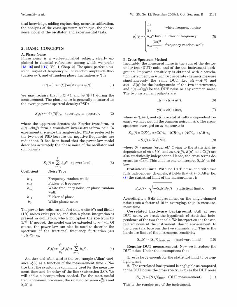
ormalism of stochastic processes [20]. Figure 3 shows anxample of OEO phase noise. The loop noise is S��f�=810−12/ f+10−14, the same used in Subsection 5.F. The pe-
iodicity of the delay-line phase produces a series of noiseeaks at frequency multiples of 1/�d. These peaks have an
+1
Φ (jf)Ψ(jf)
amplifier noise−free
resonatorB(jf)
outputinput
phase noiseoscillatorphase noise
Σ+
Fig. 2. Oscillator phase-noise model.
eswhEcln
3ATfbcmn
i�safctdwiovmsp
esclmacp
trf(cmui1atl1��tTfaTtgIscp
o�wpptltmb
ptsntlwt
BUto
Volyanskiy et al. Vol. 25, No. 12 /December 2008 /J. Opt. Soc. Am. B 2143
xtremely narrow bandwidth, in the hertz range, but inimulations and experiments they seem significantlyider because of the insufficient resolution. The peakeight follows the law S��f��1/ f4 �−40 dB/decade�.liyahu and Maleki [[21] Section 4] report about a dis-
repancy by a factor of �f �−35 dB/decade�, yet givingittle detail and suggesting that further investigation isecessary.
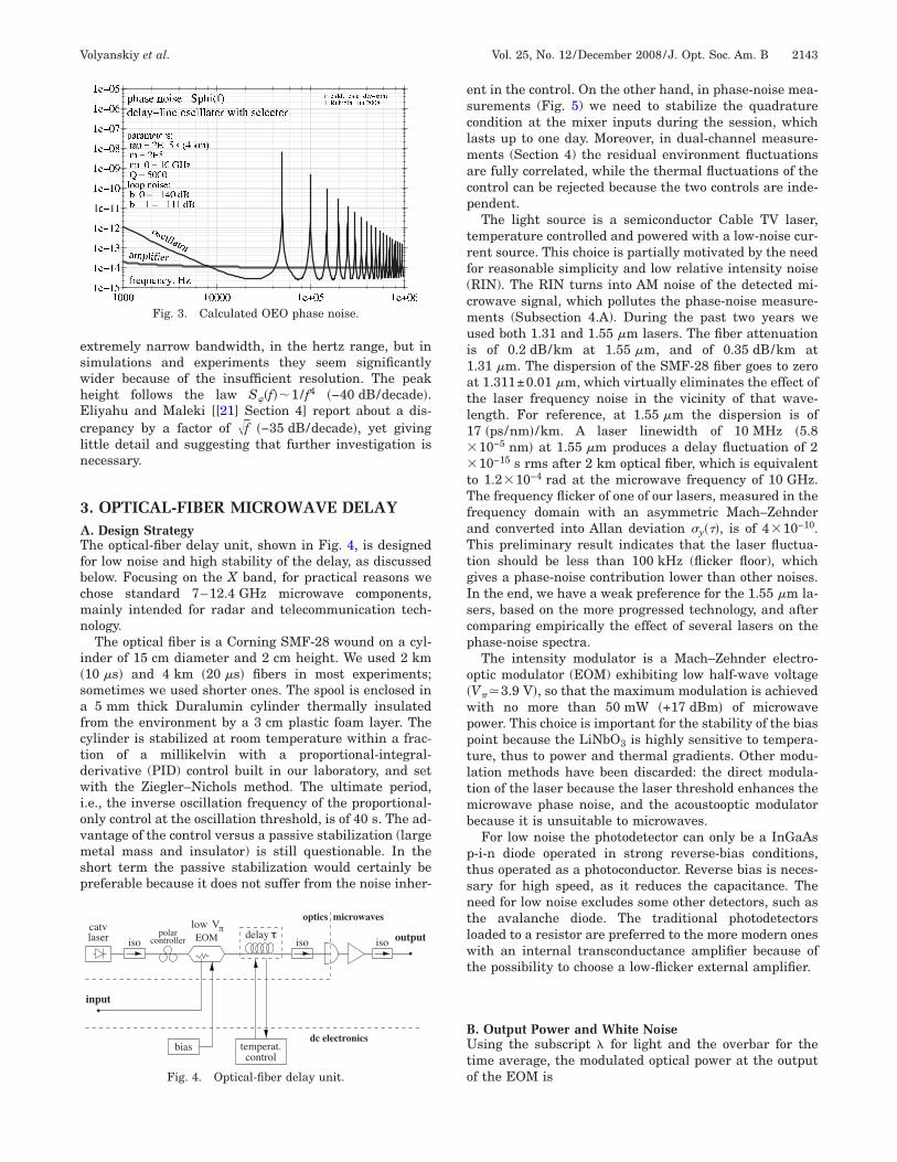
. OPTICAL-FIBER MICROWAVE DELAY. Design Strategyhe optical-fiber delay unit, shown in Fig. 4, is designed
or low noise and high stability of the delay, as discussedelow. Focusing on the X band, for practical reasons wehose standard 7–12.4 GHz microwave components,ainly intended for radar and telecommunication tech-
ology.The optical fiber is a Corning SMF-28 wound on a cyl-
nder of 15 cm diameter and 2 cm height. We used 2 km10 �s� and 4 km �20 �s� fibers in most experiments;ometimes we used shorter ones. The spool is enclosed in
5 mm thick Duralumin cylinder thermally insulatedrom the environment by a 3 cm plastic foam layer. Theylinder is stabilized at room temperature within a frac-ion of a millikelvin with a proportional-integral-erivative (PID) control built in our laboratory, and setith the Ziegler–Nichols method. The ultimate period,
.e., the inverse oscillation frequency of the proportional-nly control at the oscillation threshold, is of 40 s. The ad-antage of the control versus a passive stabilization (largeetal mass and insulator) is still questionable. In the
hort term the passive stabilization would certainly bereferable because it does not suffer from the noise inher-
Fig. 3. Calculated OEO phase noise.
dc electronics
isoVπlow
input
delay τ
temperat.control
bias
iso isolasercatv
EOMcontrollerpolar
microwavesopticsoutput
Fig. 4. Optical-fiber delay unit.
nt in the control. On the other hand, in phase-noise mea-urements (Fig. 5) we need to stabilize the quadratureondition at the mixer inputs during the session, whichasts up to one day. Moreover, in dual-channel measure-
ents (Section 4) the residual environment fluctuationsre fully correlated, while the thermal fluctuations of theontrol can be rejected because the two controls are inde-endent.The light source is a semiconductor Cable TV laser,
emperature controlled and powered with a low-noise cur-ent source. This choice is partially motivated by the needor reasonable simplicity and low relative intensity noiseRIN). The RIN turns into AM noise of the detected mi-rowave signal, which pollutes the phase-noise measure-ents (Subsection 4.A). During the past two years wesed both 1.31 and 1.55 �m lasers. The fiber attenuation
s of 0.2 dB/km at 1.55 �m, and of 0.35 dB/km at.31 �m. The dispersion of the SMF-28 fiber goes to zerot 1.311±0.01 �m, which virtually eliminates the effect ofhe laser frequency noise in the vicinity of that wave-ength. For reference, at 1.55 �m the dispersion is of7 �ps/nm� /km. A laser linewidth of 10 MHz �5.810−5 nm� at 1.55 �m produces a delay fluctuation of 210−15 s rms after 2 km optical fiber, which is equivalent
o 1.2�10−4 rad at the microwave frequency of 10 GHz.he frequency flicker of one of our lasers, measured in the
requency domain with an asymmetric Mach–Zehndernd converted into Allan deviation �y���, is of 4�10−10.his preliminary result indicates that the laser fluctua-
ion should be less than 100 kHz (flicker floor), whichives a phase-noise contribution lower than other noises.n the end, we have a weak preference for the 1.55 �m la-ers, based on the more progressed technology, and afteromparing empirically the effect of several lasers on thehase-noise spectra.The intensity modulator is a Mach–Zehnder electro-
ptic modulator (EOM) exhibiting low half-wave voltageV� 3.9 V�, so that the maximum modulation is achievedith no more than 50 mW �+17 dBm� of microwaveower. This choice is important for the stability of the biasoint because the LiNbO3 is highly sensitive to tempera-ure, thus to power and thermal gradients. Other modu-ation methods have been discarded: the direct modula-ion of the laser because the laser threshold enhances theicrowave phase noise, and the acoustooptic modulator
ecause it is unsuitable to microwaves.For low noise the photodetector can only be a InGaAs
-i-n diode operated in strong reverse-bias conditions,hus operated as a photoconductor. Reverse bias is neces-ary for high speed, as it reduces the capacitance. Theeed for low noise excludes some other detectors, such ashe avalanche diode. The traditional photodetectorsoaded to a resistor are preferred to the more modern onesith an internal transconductance amplifier because of
he possibility to choose a low-flicker external amplifier.
. Output Power and White Noisesing the subscript � for light and the overbar for the
ime average, the modulated optical power at the outputf the EOM is
w
wcvtabc=0
d0lip
w
w�fisp
Ip
Fan
CP1mf
o
aw
lb
g
Tntos
2144 J. Opt. Soc. Am. B/Vol. 25, No. 12 /December 2008 Volyanskiy et al.
P��t� = P̄��1 + mi cos�2��0t��, �18�
here the intensity-modulation index is
mi = 2J1��Vp
V�� , �19�
here J1� � is the first-order Bessel function, Vp is the mi-rowave peak voltage, and V� is the modulator half-waveoltage. Equation (19) originates from the sinusoidal na-ure of the EOM response, with Vp cos�2��0t� input volt-ge. The harmonics at frequency n�0, integer n�2, falleyond the microwave bandwidth, thus they are dis-arded. Though the maximum modulation index is mi1.164, occurring at Vp=0.586V�, the practical values are.8–1.The detected photocurrent is i�t�=�P��t�, where � is the
etector responsivity. Assuming a quantum efficiency of.6, the responsivity is of 0.75 A/W at 1.55 �m wave-ength, and of 0.64 A/W at 1.31 �m. The dc component of�t� is idc=�P̄�. The microwave power at the detector out-ut is
P0 =1
2mi
2R0�2P̄�2 �detector output�, �20�
here R0=50 � is the load resistance.The white noise at the input of the amplifier is
N = FkT0 + 2qR0�P̄� �white noise�, �21�
here F is the amplifier noise figure and kT0=410−21 J is the thermal energy at room temperature. The
rst term of Eq. (21) is the noise of the amplifier, and theecond term is the shot noise. Using b0=N /P0, the whitehase noise is
polar
input
isoatten
isoVπlow
atten
delay τlasercatv
EOM
2 km
2 km
−10 dB
−10 dB
controller
Fig. 5. Scheme of th
b0 =2
mi2�FkT0
R0
1
�2P̄�2
+2q
�P̄�� �white phase noise�.
�22�
nterestingly, the noise floor is proportional to 1/ P̄�2 at low
ower, and to 1/ P̄� above the threshold power
P� =FkT0
R0
1
2�q�threshold power�. �23�
or example, taking �=0.75 A/W and F=5 (SiGe parallelmplifier), we get a threshold of 1.7 mW, at which theoise floor is b0 10−15 rad2/Hz �−150 dBrad2/Hz�.
. Flicker Noisehase and amplitude flickering result from the near-dc/ f noise upconverted by nonlinearity or by a parametricodulation process. This is made evident by two simple
acts:
1. The 1/ f noise is always always present in the dc biasf electronic devices.
2. In the absence of a carrier, the microwave spectrumt the output of a device is white, i.e., nearly constant in aide frequency range.
Assuming that the phase modulation is approximatelyinear unless the carrier is strong enough to affect the dcias, two basic rules hold:
1. b−1 is independent of the carrier power.2. Cascading two or more devices the b−1 add up, re-
ardless of the device order in the chain.
he reader may have in mind the Friis formula for theoise referred to as the input of a chain [22], stating thathe contribution of each stage is divided by the total gainf the preceding stages, and therefore indicating the firsttage as the major noise source. The Friis formula arises
iso
iso
uadrature adjust
uadrature adjust
cs microwaves
cs microwaves
FFTanalyzer
dc
dc
-channel instrument.
iso
iso
q
q
opti
opti
e dual
fn
dhipg[am�13lo1H�
pushsbab�
ssiit
ppfmd
4MFsaiitncw
stltTFt
sgnpt[Thb
uSati1
AUnirpltd
hWUTooAflkn
i=nkpcsaasBcetsS
BTStofit
Volyanskiy et al. Vol. 25, No. 12 /December 2008 /J. Opt. Soc. Am. B 2145
rom the additive property of white noise, hence it doesot apply to parametric noise.Early measurements on amplifiers [23–25] suggest that
ifferent amplifiers based on a given technology tend toave about the same b−1, and that b−1 is nearly constant
n a wide range of carrier frequency and power. Our inde-endent experiments confirm that the 1/ f phase noise of aiven amplifier is independent of power in a wide range[26,27,19] (Chap. 2)]. For example, b−1 of a commercialmplifier (Microwave Solutions MSH6545502) that weeasured at 9.9 GHz is between 1.25�10−11 and 210−11 from 300 to 80 mW of output power. Similarly, the/ f noise of a LNPT32 SiGe amplifier measured between2 �W �−15 dBm� and 1 mW �0 dBm� in 5 dB steps over-ap perfectly. In summary, the typical phase flickering b−1f a “good” microwave amplifier is between 10−10 and0−12 rad2/Hz �−100 to −120 dBrad2/Hz� for the GaAsBTs, and between 10−12 and 10−13 rad2/Hz
−120 to −130 dBrad2/Hz� for the SiGe transistors.The 1/ f noise of the microwave photodetector is ex-
ected to be similar to that of an amplifier because thenderlying physics and technology are similar. The mea-urement is a challenging experimental problem, whichas been tackled only at the NASA–Caltech Jet Propul-ion Laboratory (JPL) (Pasadena, Calif.) independentlyy Shieh et al., [28], Shieh and Maleki [29], and Rubiola etl. [30]. The results agree in that at 10 GHz the typical−1 of an InGaAs p-i-n photodetector is of 10−12 rad2/Hz−120 dBrad2/Hz�.
Microwave variable attenuators and variable phasehifters can be necessary for adjustment. Our early mea-urements [31] indicate that the b−1 of these componentss of the order of 10−15 rad2/Hz �−150 dBrad2/Hz�, whichs negligible as compared to the amplifiers and to the pho-odetectors.
Additional sources of noise are the EOM, the laser am-lified spontaneous emission, and the noise of the opticalump. As theory provides no indications about these ef-ects, a pragmatic approach is necessary, which consists ofeasuring the total noise of the microwave delay unit in
ifferent configurations.
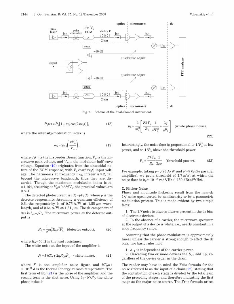
. DUAL-DELAY PHASE NOISEEASUREMENT
igure 5 shows the scheme of the instrument. Howeverimilar it is to the previous ones ([12,32]), this versiondds engineering and substantial progress in understand-ng 1/ f noise. The instrument consists of two equal andndependent channels that measure the oscillator underest using the principle of Fig. 1. Then, the single-channeloise is removed using the cross-spectrum method beforeonverting the mixer output into the oscillator noise S��f�ith Eq. (18).Looking at one channel, we observe that the microwave
ignal is split into two branches before the EOM, so thathe long branch consists of a modulator, optical fiber (de-ay �), a photodetector, and a microwave amplifier, whilehe short branch is a microwave path of negligible length.his differs from the first single-channel instrument [[10],ig. 7], in which the short branch was optical. Removinghe photodetector and the microwave amplifier from the
hort branch yields lower noise, and in turn faster conver-ence of the correlation algorithm. Lower laser power iseeded. Another advantage is that we use a microwaveower splitter instead of an optical power splitter. Whilehe noise of the former is negligible for our purposes33,34], we have no firsthand knowledge about the latter.he problem with this configuration is that we no longerave an optical input, so the microwave-modulated lighteams cannot be measured.Trading off with the available components, we had to
se both GaAs amplifiers and SiGe amplifiers. Since theiGe amplifiers exhibit lower 1/ f noise, they are insertedt the photodetector output. This choice is motivated byhe fact that the 1/ f noise at the mixer input is convertednto oscillator 1/ f3 noise by Eqs. (12) and (13) while the/ f noise at the EOM input is not.
. Mixer Noisesed as a phase detector, the double-balanced mixereeds to be saturated at both inputs. The conversion gain
s of 0.1–0.5 V/rad when the power is in the appropriateange, which is of ±5 dB centered around the optimumower of 5–10 mW. Out of this range, b−1 increases. Atower power the conversion gain drops suddenly becausehe input voltage is insufficient for the internal Schottkyiodes to switch.Out of our experience in low-flicker applications, we
ave a preference for the mixers manufactured by Nardaest (division of L3 Communications Co., New York,SA) and Marki Microwave Inc. (Morgan Hill, CA, USA).he coefficient b−1 is of the order of 10−12, similar to thatf the photodetectors. The white noise is chiefly the noisef the output amplifier divided by the conversion gain k�.ssuming that the amplifier noise is 1.6 nV/�Hz (our low-icker amplifiers input-terminated to 50 � [35]) and that�=0.1 V/rad (conservative with respect to P0), the whiteoise is b0=2.5�10−16 rad2/Hz �−156 dBrad2/Hz�.Mixers are sensitive to the amplitude noise ��t� of the
nput signal, hence the mixer output takes the form v�t�k���t�+k���t�. This is due to the asymmetry of the inter-al diodes and baluns. In some cases we have measured� /k� of 5 or less, while values of 10–20 are common. Inhotonic systems the contamination from amplitude noisean be a serious problem because of the power of some la-ers and laser amplifiers fluctuates. Brendel et al. [36]nd Cibel et al. [37] suggest that the mixer can be oper-ted at a sweet point off the quadrature, where the sen-itivity to AM noise nulls. A further study shows that therendel offset method cannot be used in our case [38] be-
ause the null of amplitude sensitivity results from thequilibrium between equal and opposite sensitivities athe two inputs. But the delay decorrelates the mixer inputignals by virtue of the same mechanism used to measure��f�.
. Calibrationhe phase-noise measurement system is governed byv�f�=k�
2�H�jf��2S��f� [Eqs. (12) and (13)]. Calibrationakes the accurate measurement of � and k�. An accuracyf 1 dB can be expected. Since the stability of the opticalber exceeds our needs, � does not need recalibration af-er the initial setup. Optical reflection methods are suit-
athtt
ecdtIsemmm
otc
wm
Ficlritk�v4tt
5ALRlne6nma
=(42afafic
BITRst(tttbp(at
Fn
Fu
2146 J. Opt. Soc. Am. B/Vol. 25, No. 12 /December 2008 Volyanskiy et al.
ble, as well as the spectrum measurement of the noisehe peak at f=1/�, where �H�jf��2=0. Conversely, k� isighly sensitive to optical and microwave power. It isherefore recommended to measure it at least every timehe experimental conditions are changed.
The simplest way to measure k� is to introduce a refer-nce sinusoidal modulation ��t�=m� sin�2�fmt� in the mi-rowave signal [Eq. (1)], after replacing the oscillator un-er test with a microwave synthesizer. This accounts forhe dc amplifier at the mixer output, not shown in Fig. 1.t is convenient to set fm�0.1/�, so that it holdsin��fm�� �fm� in Eq. (13). With commercial synthesiz-rs frequency modulation is more suitable than phaseodulation because the frequency deviation �f can beeasured in static conditions, with dc input. Frequencyodulation is equivalent to phase modulation
��t� =�f
fmsin 2�fmt, �24�
f index m�=�f / fm. Substituting Eq. (24) into Eq. (1) andruncating the series expansion to the first order, the mi-rowave signal is
v�t� = J0��f
fm�cos 2��0t + J1��f
fm��cos 2���0 + fm�t
− cos 2���0 − fm�t�, �25�
here Jn� � is the Bessel function of order n. For small�, we use the approximations J0�m�� 1 and J1�m��12m�. Thus,
v�t� = cos 2��0t +1
2
�f
fm�cos 2���0 + fm�t − cos 2���0 − fm�t�.
�26�
inally, the modulation index can be easily calibrated bynspection with a microwave spectrum analyzer. In thisase it is recommended to measure m� with relativelyarge sidebands (say, 40 dB below the carrier), and then toeduce m� by inserting a calibrated attenuator at the FMnput of the synthesizer. This enhances the accuracy ofhe spectrum analyzer. For example, having �=10 �s and�=0.2 V/rad, we may set fm=5 kHz and m�=210−2 rad. In this case, the detected signal has a peak
oltage of 400 �V at the mixer output, thus 40 mV after0 dB amplification. Measuring k�, it may be conveniento attenuate the modulating signal by 20–30 dB, so thathe system is calibrated in actual operating conditions.
. EXPERIMENTS. Measurement of the Background at Zero Fiberengtheplacing the spools of Fig. 5 with short fibers, the oscil-
ator phase noise is rejected. The noise phenomena origi-ated inside the fiber, or taken in by the fiber, are alsoliminated. The noise measured in these conditions (Fig.) is the instrument background as it would be withoise-free fibers. Curve a (red) is the phase noise S �f�easured by the mixer output. The other curves (b)–(f)
re plotted using the same data set, after inverting S �f�
v
k�2�H�jf��2S��f� for various fiber lengths [Eqs. (12) and
13)]. As expected after Subsection 2.C, curve f (black,km fiber, �=20 �s) shows a peak at 1/�=50 kHz and at/�=100 kHz, due to the division by �H�jf��2=0. Addition-lly, curve f shows two minima 6 dB lower than S �f� at=25 and 75 kHz, where �H�jf��2=4. The same phenomenare observed at twice the frequency on curve e (blue, 2 kmber, �=10 �s), although the 100 kHz peak is hidden byurve f.
. Effect of Microwave AM Noise and of Laser Relativentensity Noisehis experiment shows qualitatively the effect of the laserIN and the AM noise of the oscillator under test, still iningle-channel mode and with zero-length optical fiber, sohat the oscillator phase noise is rejected (Fig. 7). Curve 3red) is the same as curve a of Fig. 6. In this case, the op-ical source is a CATV laser, while the oscillator underest is a 10 GHz sapphire-loaded dielectric-cavity oscilla-or operated at room temperature [11]. Besides high sta-ility, the sapphire oscillator performs low AM noise. Re-lacing the laser with a different one with higher RINcurve 2, blue), or replacing the oscillator under test withsynthesizer (curve 3, black), which has higher AM noise,
ig. 7. (Color online) Effect of the laser RIN and the oscillator-nder-test AM noise, measured with zero-length fiber.
CWpsodttotbv21ts�pspre
DWiiim
o
E
ta
Nasnl
EWcspTojlqst1
ewit
Volyanskiy et al. Vol. 25, No. 12 /December 2008 /J. Opt. Soc. Am. B 2147
. Measurement of a Sapphire Microwave Oscillatore measured the phase noise of a room-temperature sap-
hire oscillator, still in single-channel mode, progres-ively increasing the fiber length (Fig. 8). The sharp peakf curve e (black) at 1/�=50 kHz and 2/�=100 kHz areue to the division by �H�jf��2=0, as explained in Subsec-ion 2.C. Of course this peak is not present in the oscilla-or noise. Let us focus on the 1/ f3 noise, which dominatesn the spectrum. When the delay is insufficient to detecthe noise of the source under test, the spectrum is theackground of the instrument, which scales with the in-erse square length, that is, −6 dB in S��f� for a factor of
in the delay. This is visible on curves a (magenta,00 m, �=0.5 �s) and b (red, 500 m, �=2.5 �s). Increasinghe length, the 1/ f3 noise no longer decreases. This fact,een on curves d (blue, 2 km, �=10 �s) and e (black, 4 km,=20 �s), indicates that the instrument measures thehase noise of the sapphire oscillator, which does notcale with the delay. Measuring the 1/ f3 noise of a sap-hire oscillator in single-channel mode is a remarkableesult because this oscillator is regarded as the best ref-rence in the field of low-noise microwave sources.
Fig. 8. (Color online) Phase noise of a sapphire oscillator.
−10 dB
input
isoatten
isoVπlow
atten
delay τlasercatv
EOM
2 km
2 km
controllerpolar
−10 dB
Fig. 9. Measurement of the backg
. Assessing the Noise of the Photonic Channele measured the phase noise of the photonic channel us-
ng the scheme of Fig. 9, derived from Fig. 5 after remov-ng some parts. The phase noise of the reference oscillators rejected by using two fibers of equal length. This experi-
ents suffers from the following limitations.
1. The noise of the fibers cannot be separated fromther noises.
2. The 1/ f noise of the GaAs amplifiers that drive theOM can show up.3. We could not use the correlation method because it
akes four matched optical delay lines, which were notvailable.
onetheless, this scheme has the merit of giving at leastn upper bound of the achievable noise. The measuredpectrum, shown in Fig. 10, indicates that the 1/ f phaseoise is b−1=8�10−12 rad2/Hz �−111 rad2/Hz�. At this
evel, the mixer noise is negligible.
. Background Noise of the Two-Channel Instrumente measured the background noise in the two-channel
onfiguration, using the cross-spectrum method of Sub-ection 2.B and with zero-length optical fiber, so that thehase noise of the 10 GHz reference oscillator is rejected.his experiment does not account for the optical noisesriginating inside the fibers; these phenomena are re-ected in Eq. (13) because the two fibers cannot be corre-ated. When this experiment was done, the stability of theuadrature condition was still insufficient for long acqui-itions. For this reason we stopped the measurement af-er m=200 spectra. The cross spectrum is shown in Fig.1.
The reference straight line (red) is the 1/ f3 phase noisequivalent to the Allan deviation �y=10−12, calculatedith Eqs. (4) and (5). Thus, averaging on 200 spectra the
nstrument can measure the stability of an oscillator athe 10−12 level.
iso
iso
cs microwaves
cs microwaves
FFTanalyzer
dc
dc
quadratureadjust
noise, including the optical fibers.
iso
iso
opti
opti
round
stssddftf
FWlwtpcctwsntmip
�edt1�t
tcs
6Ot
pmtpp2
mccdl
Fo
Ffi
Fm
2148 J. Opt. Soc. Am. B/Vol. 25, No. 12 /December 2008 Volyanskiy et al.
The signature of a correlated noise is a smooth crosspectrum. Yet, in Fig. 11 the variance is far too large forhe two channels to be correlated. This indicates that theensitivity is limited by the small number of averagedpectra. Additionally, the spectrum shows a sawtoothlikeiscrepancy versus the 1/ f3 line. This averaging effect,ue to the measurement bandwidth that increases withrequency in logarithmic resolution, further indicates thathe value of m is still insufficient. The ultimate sensitivityor large m is still not known.
. Opto-Electronic Oscillatore implemented the oscillator of Fig. 12 using a 4 km de-
ay line �20 �s�, a SiGe amplifier, and a photodetectorith an integrated transconductance amplifier. Oscilla-
ion starts at 6–7 mW optical power. The best workingoint occurs at 12–13 mW optical power, where the mi-rowave output power is 20 mW. For flicker noise the mi-rowave chain is similar to one channel in Fig. 9 becausehe order of the devices in the chain is not relevant. Thus,e take b−1=8�10−12 rad2/Hz �−111 dBrad2/Hz�, the
ame as that of Fig. 10, as the first estimate of the loopoise. Though somewhat arbitrary, this value accounts forhe photodetector internal amplifier, more noisy than ouricrowave amplifiers. Using �b−1�loop=8�10−12 rad2/Hz
n the oscillator noise model of Subsection 2.D, the ex-ected oscillator flickering is �b−3�osc=6.3�10−4 rad2/Hz
ig. 10. (Color online) Background noise, including the opticalbers.
ig. 11. (Color online) Background noise in two-channel mode,easured with zero-length fiber.
−32 dBrad2/Hz�. By virtue of Eq. (4) and (5), this isquivalent to a frequency stability �y=2.9�10−12 (Allaneviation). The noise spectrum (Fig. 13), measured withhe dual-channel instrument, shows a frequency flicker of0−3 rad2/Hz �−30 dBrad2/Hz�, equivalent to �y=3.610−12. The discrepancy between the predicted value and
he result is 2 dB.Interestingly, the OEO phase noise compares favorably
o the lowest-noise microwave synthesizers and quartz os-illator multiplied to 10 GHz. Yet, the OEO can bewitched in steps of 50 kHz without degrading the noise.
. FURTHER DEVELOPMENTSur experiments suggest the following improvements,
ested or in progress.
1. In the phase-noise instrument, the microwaveower the input of the EOM and the two inputs of theixer is a critical parameter because the gain of the en-
ire system is strongly nonlinear. The insertion of testoints is recommended, using common and inexpensiveower detectors after tapping a fraction of the power with0 dB directional couplers.2. The instrument requires that the two signals at theixer input are kept in quadrature. This is usually ac-
omplished with a line stretcher or a with voltage-ontrolled phase shifter. A smarter solution exploits theispersion of the optical fiber by adjusting the laser wave-ength via the temperature control [39]. This is viable
Fig. 12. Scheme of the optoelectronic oscillator.
ig. 13. (Color online) Phase noise of the optoelectronicscillator.
oacAtw�
ttb
Rttt
AWCCwCfCFBTshci
C
R
1
1
1
1
1
1
1
1
1
1
2
2
2
2
2
2
2
2
2
2
3
3
Volyanskiy et al. Vol. 25, No. 12 /December 2008 /J. Opt. Soc. Am. B 2149
nly at 1.55 �m and with long fibers. For reference, using2 km fiber and our lasers, it takes 10 K of temperature
hange for a quarter wavelength of the microwave signal.nother solution exploits the temperature coefficient of
he fiber delay, 6.85�10−6/K. Accordingly, a quarteravelength takes 0.37 K of temperature with 2 km fiber
10 �s�, or 3.7 K with 200 m.3. Some popular EOMs have a low-frequency photode-
ector at the unused output port of the Mach–Zehnder in-erferometer, which we hope to exploit to stabilize theias point.4. The OEO frequency can be fine-tuned by adding a
F signal with an SSB modulator at the output. Ex-remely high resolution, of the order of 10−16, can be ob-ained with a 48 bit DDS, with no degradation of the spec-ral purity [40,41].
CKNOWLEDGMENTSe are indebted to Lute Maleki [OEwaves and NASA–altech (JPL), Pasadena, Calif., USA], Nan Yu (NASA/altech JPL) and Ertan Salik (NASA–Caltech JPL, nowith the California State Polytechnic University, Pomona,alif., USA) for having taught us a lot in this domain, and
or numerous discussions, advice, and exchanges. Gillesibiel (Centre National d’Etudes Spatiales (CNES),rance) provided contract support and help. Rodolpheoudot (FEMTO-ST, now with Systèmes de Reférénceemps-Espace (SYRTE), Paris, France) helped with theapphire oscillator, Xavier Jouvenceau (FEMTO-ST)elped in the implementation of the early version of theorrelation system, and Cyrus Rocher (FEMTO-ST)mplemented the temperature control.
This work is supported with grants from Aeroflex,NES, and Agence Nationale de la Recherche (ANR).
EFERENCES1. W. S. C. Chang, ed., RF Photonic Technology in Optical
Fiber Links (Cambridge U. Press 2002).2. T. A. Yilmaz, C. M. Depriest, A. Braun, J. Abeles, and P. J.
Delfyett, “Noise in fundamental and harmonic modelockedsemiconductor lasers: experiments and simulations,” IEEEJ. Quantum Electron. 39, 838–849 (2003).
3. D. J. Jones, K. W. Holman, M. Notcutt, J. Ye, J. Chandalia,L. A. Jiang, E. P. Ippen, and H. Yokoyama, “Ultralow-jitter,1550-nm mode-locked semiconductor laser synchronized toa visible optical frequency standard,” Opt. Lett. 28,813–815 (2003).
4. X. S. Yao and L. Maleki, “Optoelectronic microwaveoscillator,” J. Opt. Soc. Am. B 13, 1725–1735 (1996).
5. X. S. Yao, L. Davis, and L. Maleki, “Coupled optoelectronicoscillators for generating both RF signal and opticalpulses,” J. Lightwave Technol. 18, 73–78 (2000).
6. K. J. Vahala, “Optical microcavities,” Nature 424, 839–846(2003).
7. T. J. Kippenberg, S. M. Spillane, and K. J. Vahala, “Kerr-nonlinearity optical parametric oscillation in anultrahigh-Q toroid microcavity,” Phys. Rev. Lett. 93,083904 (2004).
8. A. A. Savchenkov, A. B. Matsko, D. Strekalov, M. Mohageg,V. S. Ilchenko, and L. Maleki, “Low threshold opticaloscillations in a whispering gallery mode caf2 resonato,”Phys. Rev. Lett. 93, 1–4 (2004).
9. S. T. Cundiff and J. Ye, “Colloquium: femtosecond opticalfrequency combs,” Rev. Mod. Phys. 75, 325–342 (2003).
0. E. Rubiola, E. Salik, S. Huang, and L. Maleki, “Photonicdelay technique for phase noise measurement of microwaveoscillators,” J. Opt. Soc. Am. B 22, 987–997 (2005).
1. V. Giordano, P.-Y. Bourgeois, Y. Gruson, N. Boubekeur, R.Boudot, E. Rubiola, N. Bazin, and Y. Kersalé, “Newadvances in ultra-stable microwave oscillators,” Eur. Phys.J.: Appl. Phys. 32, 133–141 (2005).
2. E. Salik, N. Yu, L. Maleki, and E. Rubiola, “Dual photonic-delay-line cross correlation method for the measurement ofmicrowave oscillator phase noise,” in Proceedings of theEuropean Frequency Time Forum and Frequency ControlSymposium Joint Meeting (2004), pp. 303–306.
3. J. Rutman, “Characterization of phase and frequencyinstabilities in precision frequency sources: fifteen years ofprogress,” Proc. IEEE 66, 1048–1075 (1978).
4. H. G. Kimball, ed., Handbook of Selection and Use ofPrecise Frequency and Time Systems (ITU, 1997).
5. CCIR Study Group VII, Characterization of Frequency andPhase Noise, Report No. 580-3, in Standard Frequenciesand Time Signals, Vol. VII (annex) of Recommendationsand Reports of the CCIR (International TelecommunicationUnion, 1990), pp. 160–171.
6. J. R. Vig (chair.), IEEE Standard Definitions of PhysicalQuantities for Fundamental Frequency and TimeMetrology-Random Instabilities IEEE Standard 1139-1999(IEEE, 1999).
7. J. Vanier and C. Audoin, The Quantum Physics of AtomicFrequency Standards (Hilger, 1989).
8. E. Rubiola, “The Leeson effect,” arXiv:physics/0502143v1,web site arxiv.org (2005). Abridged draft version of [19].
9. E. Rubiola, Phase Noise and Frequency Stability inOscillators (Cambridge U. Press, 2008).
0. Y. K. Chembo, K. Volyanskiy, L. Larger, E. Rubiola, and P.Colet, “Determination of phase noise spectra inoptoelectronic microwave oscillators: a phase diffusionapproach,” J. Quantum Electron. (to be published).
1. D. Eliyahu and L. Maleki, “Low phase noise and spuriouslevel in multi-loop opto-electronic oscillators,” inProceedings of the European Frequency Time Forum andFrequency Control Symposium Joint Meeting (2003), pp.405–410.
2. H. T. Friis, “Noise figure of radio receivers,” Proc. IRE 32,419–422 (1944).
3. D. Halford, A. E. Wainwright, and J. A. Barnes, “Flickernoise of phase in RF amplifiers: characterization, cause,and cure,” (Abstract) in Proceedings of Freqency ControlSymposium (1968), pp. 340–341.
4. F. L. Walls, E. S. Ferre-Pikal, and S. R. Jefferts, “Origin of1/ f PM and AM noise in bipolar junction transistoramplifiers,” IEEE Trans. Ultrason. Ferroelectr. Freq.Control 44, 326–334 (1997).
5. A. Hati, D. Howe, D. Walker, and F. Walls, “Noise figure vs.PM noise measurements: a study at microwavefrequencies,” in Proceedings of the European Freqency TimeForum and Freqency Control Symposium Joint Meeting(2003).
6. E. Rubiola and R. Boudot, “1/ f noise of RF and microwaveamplifiers,” available soon on http://arxiv.org.
7. R. Boudot, “Oscillateurs micro-onde à haute puretéspectrale,” Ph.D. dissertation (Université de FrancheComté, 2006).
8. W. Shieh, X. S. Yao, L. Maleki, and G. Lutes, “Phase-noisecharacterization of optoelectronic components by carriersuppression techniques,” in Proceedings of the OpticalFiber Communication (OFC) Conference (1998), pp.263–264.
9. W. Shieh and L. Maleki, “Phase noise characterization bycarrier suppression techniques in RF photonic systems,”IEEE Photon. Technol. Lett. 17, 474–476 (2005).
0. E. Rubiola, E. Salik, N. Yu, and L. Maleki, “Flicker noise inhigh-speed p-i-n photodiodes,” IEEE Trans. MicrowaveTheory Tech. 54, 816–820 (2006).
1. E. Rubiola, V. Giordano, and J. Groslambert, “Very high
3
3
3
3
3
3
3
3
4
2150 J. Opt. Soc. Am. B/Vol. 25, No. 12 /December 2008 Volyanskiy et al.
frequency and microwave interferometric PM and AM noisemeasurements,” Rev. Sci. Instrum. 70, 220–225 (1999).
2. P. Salzenstein, J. Cussey, X. Jouvenceau, H. Tavernier, L.Larger, E. Rubiola, and G. Sauvage, “Realization of a phasenoise measurement bench using cross correlation anddouble optical delay line,” Acta Phys. Pol. A 112, 1107–1111(2007).
3. E. Rubiola and V. Giordano, “Correlation-based phase noisemeasurements,” Rev. Sci. Instrum. 71, 3085–3091 (2000).
4. E. Rubiola and V. Giordano, “Advanced interferometricphase and amplitude noise measurements,” Rev. Sci.Instrum. 73, 2445–2457 (2002).
5. E. Rubiola and F. Lardet-Vieudrin, “Low flicker-noiseamplifier for 50 � sources,” Rev. Sci. Instrum. 75,1323–1326 (2004).
6. R. Brendel, G. Marianneau, and J. Ubersfeld, “Phase and
amplitude modulation effects in a phase detector using an 4
7. G. Cibiel, M. Régis, E. Tournier, and O. Llopis, “AM noiseimpact on low level phase noise measurements,” IEEETrans. Ultrason. Ferroelectr. Freq. Control 49, 784–788(2002).
8. E. Rubiola and R. Boudot, “The effect of AM noise oncorrelation phase noise measurements,” IEEE Trans.Ultrason. Ferroelectr. Freq. Control 54, 926–932 (2007).
9. K. Volyanskiy and L. Larger, Quadrature Stabilization inthe Opto-Electronic Phase-Noise Measurement System byLaser Tuning, FEMTO-ST internal report (FEMTO-ST,2008), personal communication.
0. Elisa—Technical Notes of the ESA Cryo Project, Series ofFEMTO-ST and ESA internal reports (FEMTO-ST, 2007-2008).