Applications of Time Synchronized Measurements in the Electric Grid Mohini Bariya Electrical Engineering and Computer Sciences University of California, Berkeley Technical Report No. UCB/EECS-2021-196 http://www2.eecs.berkeley.edu/Pubs/TechRpts/2021/EECS-2021-196.html August 13, 2021
Transcript
Applications of Time Synchronized Measurements in
the Electric Grid
Mohini Bariya
Electrical Engineering and Computer SciencesUniversity of California, Berkeley
Permission to make digital or hard copies of all or part of this work forpersonal or classroom use is granted without fee provided that copies arenot made or distributed for profit or commercial advantage and that copiesbear this notice and the full citation on the first page. To copy otherwise, torepublish, to post on servers or to redistribute to lists, requires prior specificpermission.
Applications of Time Synchronized Measurements in the Electric Grid
by
Mohini Bariya
A dissertation submitted in partial satisfaction of the
requirements for the degree of
Doctor of Philosophy
in
Engineering – Electrical Engineering and Computer Sciences
in the
Graduate Division
of the
University of California, Berkeley
Committee in charge:
Professor Kannan Ramchandran, Co-chairAdjunct Professor Alexandra von Meier, Co-chair
Associate Professor Prabal DuttaProfessor Scott Moura
Summer 2021
Applications of Time Synchronized Measurements in the Electric Grid
Copyright 2021by
Mohini Bariya
1
Abstract
Applications of Time Synchronized Measurements in the Electric Grid
by
Mohini Bariya
Doctor of Philosophy in Engineering – Electrical Engineering and Computer Sciences
University of California, Berkeley
Professor Kannan Ramchandran, Co-chair
Adjunct Professor Alexandra von Meier, Co-chair
Increased real-time monitoring of the electric grid is vital to meet the burgeoning challengesposed by load growth and diversification, renewable generation integration, extreme weatherevents, and cyber attacks. Grid operators must have situational awareness—an understand-ing of the system’s evolving state—if they are to respond appropriately to challenging andchanging system conditions. The proliferation of measurement devices in the electric grid iscritical for situational awareness, but is not su�cient: measurements need to be convertedto actionable insight to be useful. Here, computational tools that ingest measurements toinfer system parameters and state are critical. While many such tools have been proposedin the research literature, their real-world use is limited, resulting in a circumstance whereballooning volumes of measurements are perceived as overwhelming rather than insightful,diminishing the incentive for further sensor deployments.This thesis argues for the creation of usable tools to bridge the chasm between researchand deployment. Usable tools have practically realizable data input requirements and—intheir forms and outputs—work in e↵ective collaboration with human users. Such tools arewell-suited to the demands of real grids, where data and prior knowledge remain scarce, andwhere safety critical decisions involve human participants.The thesis goes on to describe several usable tool algorithms for the use cases of topologyestimation and monitoring, event detection, and event classification. Finally, it presentsbroad principles for the further development of usable tools.Throughout, the thesis emphasizes how high resolution, time synchronized measurementsare particularly enabling for the creation of usable tools.
A C K N O W L E D G E M E N T S
Reader: the acknowledgements are the first part you read but the final partI write of this thesis. At this very last step of my PhD, I am filled withgratitude—and a sense of immense good luck—reflecting on the peoplewho helped me get here.Many thanks to my wonderful advisor, Sascha von Meier, for her insight,good spirits, kindness, and unrelenting support. I have been uplifted afterevery meeting with her. My co-advisor Kannan Ramchandran was alwaysgenerous with his time and always engaged and enthusiastic to discuss mywork, no matter how distant the application from his everyday preoccupa-tions. I ensnared my committee members Prabal Dutta and Scott Mourabefore my qualifying exam, and since then I have benefited from their feed-back, guidance, and good nature.Two people set me on the way when I was a young student with no idea ofwhat to do or why: Michael Cohen, who introduced me to the electric grid,and Professor Jeffrey Hadler, who will always be my model of humanity,compassion, and grace.I can confidently assert that I had the best group mates possible. I com-mend Sascha for collecting them; we are lifelong friends! Immense thanksto Keith Moffat, Jaimie Swartz, Gabriel Colon-Reyes, Kyle Brady, MilesRusch and Laurel Dunn for joyous times at work and outside. Thanks alsoto my many wonderful colleagues, collaborators, and comrades: Jonny Lee,Aminy Ostfeld, Liz Ratnam, John Paparrizos, Deep Deka, Sean Murphyand K.S. Sajan. Their insights and assistance were crucial to my learningand this work. I must thank Betsy Mitchell for the happy summer hoursworking (and carpooling) together. A special thanks to Alex McEachernwhose extraordinary perspicacity is matched by his enormous kindness.Thanks to my dear Berkeley friends, who have stoically tolerated my erraticresponsiveness to texts and yet are always available for me: Amit Akula,Christine Vandevoorde and Linus Kipkoech, Nicholas Gan, Kai-Sern Lim,Rebecca Pak, Nick Chang, Bala Kumaravel, Vignesh Subramanian, andHarkiran Kaur Sodhi. I have so many fond memories of days and evenings
i
ii
together, and look forward to our reunions in Berkeley and elsewhere. Par-ticular thanks to the people that became my covid community: Henry Tengand my betas, Varun and Kahaan Maniar. We cooked, imbibed, traveledand, above all, laughed uncontrollably together!Boundless thanks to my wonderful family, near and far. Thanks to myloving grandparents: Ba —who left us too soon —Nani, Nana, and Dada.Thanks to the Bariya cousins —Amol, Aman, Mohit, and Anooj —withwhom were the happiest moments of my childhood. To Monica, Mad-havi, Apu, Lalana, and Sonali—how many are fortunate enough to have somany lovely and loving aunts—and my uncles. In Berkeley, thanks to Venfor great times and support, and to Danny for conversation and kindnessover dinner and during my unannounced visits. And last thanks to mynewest family member: Sabrina.Perhaps strangely there are places I must thank, that kept me going andgave me meaning. India is always on my mind and in my heart. I willnever forget my few days at Merced National Wildlife Refugee, watchingat dawn and dusk thousands of sandhill cranes dancing and calling andflying together over the misty lake. My work is for these places.While writing this thesis, I enjoyed the literary company of Martin Amisin Inside Story. Reading his passages made me mindful of my own. Hisadvice —on picking the right word, avoiding repetition, eschewing thecanned phrase and being conscious of the cadence of paragraphs —I havetried, though not fully managed, to follow. Nevertheless, I, and my reader,owe him thanks.Finally, and most significantly: thanks to my jigri doston, my soul friends,Eugene Kang and Sourav Ghosh. I can not express how much happinessand joy you have brought me. I look forward to growing old together, sit-ting on tropical verandahs, sipping g&ts and listening to music (k-pop andqawwali) over endless conversations and laughter.And above all and always, thanks to the humsafars, the travel companions,of my life: Ilias, my sister Mallika, and my parents Anand and Suhag, whoknow me better than I know myself. This thesis is dedicated to them.
C O N T E N T S
� ������������ 11.1 The Electric Grid 11.2 Motivation 41.3 Contribution 71.4 Notation 8
� ���� ��� ������ �����? 353.1 Tools in the Literature 403.2 Tools in Industry 463.3 The Gap 493.4 Bridging the Gap: Usable Tools 513.5 The Future Toolbox 56
� �������� ����� 604.1 Towards usable tools for topology 634.2 A Heuristic Approach 654.3 A Physics Approach 774.4 Extension to Three Phase Networks 1044.5 Justified Heuristics 124
� ���������� ��� ������ ����� 1646.1 Linear Models 1646.2 Statistical Assumptions 1676.3 Statistical Baselines 1696.4 A Vision for Tools 170������������ 171
iii
1 I N T R O D U C T I O N
�.� ��� �������� ����Electric grids deliver energy in the form of electricity from generators toconsumers. Beside this unifying feature, electric grids are diverse, and anygeneral description will likely be violated by some grid, somewhere. Insize, grids range from gigantic to small. The contiguous European gridspans east to west from Portugal to Turkey and north to south from Alge-ria to the Netherlands. At the opposite scale, a grid may encompass just asingle generator and a few small loads, supplying energy to an industrialpark or to an isolated village. Most grids, and certainly all substantial ones,deal in alternating current (ac) power, with voltages and currents that varysinusoidally in time. Yet, an increasing number of grids are direct current(dc) systems, with constant steady state voltages and currents. A mixture ofac and dc elements is also possible. Some grids may rely on a single gener-ation source or even a single generator, but most large grids include variedgenerator types. The Brazilian grid incorporates enormous hydropowerplants alongside gas, nuclear, and oil generators while the European gridencompasses Spanish solar farms, French nuclear plants and German off-shore wind turbines. Energy user, or load, types are even more diversethan generators, ranging from households with lighting and appliances toenergy-hungry factories and, today, giant data centers. In between gener-ators and loads, a large grid includes thousands of pieces of equipmentfor smooth and safe operations. Lines carry current, transformers changevoltage levels, switches reconfigure connections while breakers open themin response to unsafe conditions, and all the while meters measure cus-tomer consumption. Consequently, the grid and those who work on it arethe elephant and the blind men in the famous parable: each participantfocuses on a particular aspect of the system from the perspective of theirparticular priorities. A grid planner considers financing and infrastructureon time scales of years or decades, an operator thinks of markets for balanc-
1
�.� ��� �������� ���� 2
Figure 1: Satellite imagery of the Earth at night captures much about the electricgrid: its scale, extent, and inequities but most vividly its fundamentalimportance to modern life [1].
ing demand and supply every hour, a protection engineer is preoccupiedwith the coordination of fuses on a particular circuit, an analyst considersthe geopolitical implications of an international grid interconnection, anda politician worries about election impacts of expanding infrastructure tounderserved constituents.In a contiguous ac grid these disparate elements are bound by the singlefrequency of sinusoidal voltages and currents across the system. This fre-quency originates in the grid’s heart(s)—the massive rotating turbines ofgenerators—and is a pulse measurable everywhere, leading such grids tobe termed synchronous. For this reason, despite the numerous elements con-stituting the grid, we can believably describe it as a single machine: “theworld’s largest machine". Historically, beneficial economies of scale havedriven synchronous grids to be larger and larger, aggregating customersto be supplied by enormous, centralized power plants. From these plants,energy flows unidirectionally outward through the system to consumers,whose demand is considered inflexible, and in aggregate follows consis-tent patterns. This operational regularity, and the physics of synchronousgenerators have given synchronous grids surprising stability and robust-ness despite minimal sensing and meager temporal and spatial flexibility
�.� ��� �������� ���� 3
or visibility into the system state. Built out incrementally over decades intoenormous, complex infrastructures, synchronous grids have worked underlittle real time management or even understanding, conveyed in the pithymaxim: “the electric grid works in practice but not in theory".Synchronous grids are organized and operated in two, mostly silo-ed parts:transmission and distribution. Transmission networks carry bulk power—at high voltages to minimize losses—over the long distances from central-ized generators to loads. Transmission infrastructure is large, with talltowers and hefty lines. This is the most visible portion of the electric gridboth physically and operationally. Who can fail to notice transmissionlines traversing the landscape between imposing towers? For operators,relatively high sensor deployments and network information provide vis-ibility into the operating state of transmission. This enables a degree ofcontrol and optimization in transmission: for example, using network con-nectivity and impedances, optimal power flows can be solved to set gener-ator outputs that minimize losses or cost. Nevertheless, even in transmis-sion, real time visibility is surprisingly low, as illustrated by two examples.First, in many transmission networks, ac voltages at nodes are not directlymeasured but must be estimated through a process called state estima-tion, with non-negligible error. Second, the loading limits of transmissionlines—which constrain the quantities of power they can transfer—changedynamically with weather conditions, but are usually known only stati-cally, leading to overly conservative line usage.Distribution is isolated from transmission through transformers, which re-duce transmission level voltages to the lower and safer ones at which poweris delivered to most loads. In total distance covered, distribution networksconstitute the bulk of the electric grid. Yet it is easier to overlook the infras-tructure of distribution which is smaller and sometimes even underground.Analogously, operational visibility into distribution is rudimentary, andcontrol generally consists of automated and invariable protection devices,set to respond only to extreme events. Often, even basic parameters of dis-tribution networks—such as their connectivity structures—are erroneousor not known. Problematically, distribution is also the more vulnerablepart of the grid: highly exposed to tree falls, animal contact, storms andeven unwitting or malicious human damage.What grid management does occur takes place largely in control rooms:themselves separated into transmission and distribution. Here human gridoperators monitor the system, much like in air traffic control, hands ready
�.� ���������� 4
at phones to communicate with field workers or respond to customer re-ported outages. They are surrounded by system information, previously inthe form of paper reports updated manually after field visits and increas-ingly as screens displaying measurements streaming in from field devices.The grid is so enormous, that even with paltry system visibility, controlrooms are sites of information overload. Those who work with grid dataknow the difficulty of interpreting measurements from just a single gridsensor. In contrast, operators must synthesize multiple sources and typesof information to inform critical decisions, with little automated assistance.This is already an onerous task today, though current levels of grid dataand measurement fall far short of those required for complete system visi-bility.Despite the existing challenges spanning transmission, distribution, andcontrol rooms, the electric grid in the developed world was long consid-ered a “solved problem”. Grid reliability is high: for example, on averagein the United States in 2013, customers endured less than three hours ofinterruptions per year [2]. Customers in western Europe fared even better[3]. How is this possible? As mentioned, synchronous generators and thehistoric regularity of loads contribute to system stability. In addition, gridinfrastructure in the developed world has been oversized and overbuilt, al-lowing operators to abide by extra cautious system limits. The result isa reliable yet inflexible and (cumulatively) costly system which strays lit-tle from the expected operating state and therefore requires minimal realtime visibility. Reliability is further enhanced through expensive infrastruc-ture choices. In Germany, for example, extensive undergrounding of linesreduces distribution grid vulnerability and outages enormously, albeit athigh cost [4].In the years ahead, this legacy operational model for electric grids will behighly challenged and even infeasible in many contexts. In light of daunt-ing new demands and difficulties facing the system, a new approach togrid management is needed, as are novel tools to enable it.
�.� ����������The looming challenges facing electric grids arise from a conjunction ofnew trends and old approaches. The legacy approach to running grids—
�.� ���������� 5
as rigid, opaque, oversized systems—-is unviable as loads and generationgrow and diversify, and new security concerns emerge.The diversification of loads and generation is due in part to transforma-tions external to the energy sector: an example is the growth of electricityusage by computers in data centers. However, the primary driver of diversi-fication is the accelerating global effort to decarbonize our energy systemsin order to mitigate the devastating impacts of climate change. Electrifyingtechnologies and processes that have historically depended on fossil fuelsis an important first step toward curtailing carbon emissions. Currently,transportation accounts for 14% of global CO2 emissions [5], motivatingcountries across the developed and developing world to set ambitious elec-tric vehicle (EV) adoption targets [6]. Industrial production is another ma-jor carbon emitter, and the electrification of industry, though especiallytechnically challenging, is recognized as essential for meeting global cli-mate targets [7]. Consequently, electrified industrial plants and vehiclesare increasingly being plugged into the grid. The integration of these newload types strains the electric grid in diverse ways. Novel loads may intro-duce unprecedented dynamics and usage trends, challenging the expertiseof grid operators and engineers as they plan and run the system. Forexample, the operation of industrial equipment is often the cause of trou-blesome disturbances in transmission networks; these will only increaseas more industrial plants are electrified. Another example: research sug-gests that long used, well established load models—vital components ofpower system planning and operation studies—do not adequately capturethe behaviors of novel loads [8]. The location of novel loads presents addi-tional challenges. Many novel loads will be connected to the grid throughthe distribution network, the most opaque portion of the system that isneither designed nor managed to handle the behaviors of such loads. Dis-tribution power quality issues—permissibly overlooked in the past—mayhave serious consequences on novel loads, which could in turn amplifythese local problems into system-wide ones. For example, short, signifi-cant dips in network voltage—termed “voltage sags”—are inconsequentialto lightbulbs or ovens but may cause EV chargers to trip offline [9]. Thecoincident tripping of numbers of EV chargers can exacerbate distributionvoltage problems and even destabilize the broader grid.On the generation side, decarbonization efforts are propelling the integra-tion of renewable energy in the grid. Renewable generators encompass arange of energy sources—wind, water, sunlight—and technologies. They
�.� ���������� 6
differ widely in scale and character. Hydro generation is usually large scalein the form of dams, while wind and especially solar can range in sizefrom individual household installations to farms covering many squarekilometers. From the grid perspective, the challenge of integrating renew-able sources has spatial and temporal dimensions. Renewable availabilityis spatially varied and inflexible. Places with high renewable generationpotential tend to be distant from locations of significant energy demand.To utilize this potential, grid infrastructure must carry more power overlonger distances. Another spatial problem arises from where renewablegeneration interconnects to the grid. Power generated by rooftop solarpanels enters the grid in the distribution network—a system which wasnot designed to expect the resulting, sometimes bidirectional, power flows.Meanwhile, the temporal challenge of renewables is that their outputs, un-like those of fossil fuel power plants, vary in uncontrollable and largelyunpredictable ways. In power systems—which lack significant storage yetmust precisely balance generation and load—this unpredictable temporalvariability is a grave challenge. Similar to novel load types, renewable gen-eration technologies have behaviors unforeseen by grid designers whichcan challenge conventional approaches to safety and stability. A com-pelling example is the Blue Cut fire incident in California, where a faultevent caused 1.2 GW of rooftop solar to suddenly trip offline, resulting ina large system disturbance [10]. The trip was incited by the controllers ofthe inverters which interface between rooftop solar systems and the bulkgrid, and whose rapid control schemes are generally unknown to and un-accounted for by grid operators. At a wider scale, the displacement ofgenerators with enormous turbines by power electronic based renewabletechnologies leads to less of the inertia that allows the grid to ride throughsmall discrepancies in generation and demand and to maintain a systemfrequency that deviates little from nominal.Weather poses another challenge. The grid, like us, is vulnerable to theimpacts of climate change. More extreme, more volatile weather—in theform of wildfires, floods, and storms—damages grid infrastructure, lead-ing to more frequent, longer outages. In turn, grid responses to extremeweather can exacerbate the human toll of these events. Some examplesfrom the United States highlighting the deleterious interplay between ex-treme weather and the electric grid are the infrastructure damage andlong-duration power outages experienced by Puerto Rico in the wake ofHurricane Maria, the California wildfires sparked by grid failures during
�.� ������������ 7
extreme heat and ensuing public safety power shutoffs, and the freakishcold weather that forced power plants offline resulting in blackouts andsurging prices in Texas [11]–[13].A final, emerging concern for electric grids is the threat of malicious attacksby entities seeking to disable this vital infrastructure. The proliferationof networked devices and automation in electric grids can increase theirvulnerability to cyber attacks. Given their importance to most aspects ofmodern life, electric grids are relatively unprotected from attackers. Gridcyber attacks have already occurred: a 2015 attack in Ukraine led to loss ofpower for over 200, 000 people [14]. The risk of such attacks will only growin the years ahead.
�.� ������������The first, critical step to address the increased threats, faster changing con-ditions, and greater complexity emerging in all parts of the electric grid, isimproved real-time visibility across the system. This is especially necessaryin distribution networks, which are traditionally managed as passive andtherefore opaque systems. Before grid engineers and operators can beginto concern themselves with how to respond to challenging conditions, theymust be aware of the conditions, and of the broader system context. Theymust have what is termed situational awareness: a sufficient understandingof the system’s status to inform an appropriate response. However, obtain-ing situational awareness is complicated by two realities: the lack of com-prehensive data availability and the challenge for a human to understandeven the limited data coming from such a massive and complex system.This thesis argues for the creation of computational tools that provide aware-ness of important system parameters and occurrences to human users. Thetools must derive operational insight from measurements, especially byleveraging the beneficial traits of high-resolution, time synchronized gridmeasurements. The tools must transform overwhelming volumes of datato a scale and form suitable for human comprehension. Grid monitoringtools have been developed in the past for various use cases, but most havefailed to percolate from research to application. This thesis argues that fortools to be operationally useful, they must meet the criteria of usability, en-compassing practical deployment requirements and human interpretability.
�.� �������� 8
The thesis then presents work on usable tool development for several usecases.The rest of the thesis is organized as follows.
• Chapter 2 presents the technical foundations for the creation of gridmonitoring tools. These foundations consist of high-resolution, timesynchronized measurements from novel grid sensors and the compu-tational platforms that enable the performant storage and access ofthis data.
• Chapter 3 surveys the literature of grid monitoring tools to under-stand broad, common features and postulate why most tools fail totransfer to application. Goaded by this survey, the chapter then pro-poses a succinct set of criteria for usable tools, arguing that tools whichmeet these criteria are well-suited to the needs of real-world deploy-ment.
• Chapter 4 presents several tools for the use case of topology monitor-ing, highlighting how the tools represent a progress toward increas-ing usability.
• Chapter 5 presents usable tools for event detection and classification.
• Chapter 6 draws together the lessons from prior chapters to presentfundamental principles and strategies for designing usable grid mon-itoring tools. The chapter emphasizes how high-resolution, time syn-chronized measurements are especially empowering for the creationof usable tools.
�.� ��������To the best of our ability, we try to maintain consistent notation through-out this work. Scalar quantities are denoted in lowercase, while vector andmatrix quantities are denoted in uppercase. Boldface indicates complex val-ued quantities, while real quantities are non-bold. Uppercase, calligraphicletters, such as N, denote sets. We use j for the imaginary unit to avoidconfusion with electric current: j =
p-1. In the electric grid, quantities
are often expressed in per-unit (pu), in which the raw value is standardizedby nominal level. Therefore, a voltage of 1200 V on a line with a nominal
�.� �������� 9
voltage of 1 kV is expressed as 1.2 pu. There are a smattering of per-unitvalues in this thesis.The table below contains a basic demonstration of the notation used. Restassured that notation will be defined and reiterated in each section.
x real-valued scalarx complex-valued scalarX real-valued matrixX complex-valued matrixXij i,j element of matrix X
2 F O U N DAT I O N S
Includes work from [15]–[17]
Novel tools for grid monitoring and management are built on a founda-tion of grid measurements and the computing platforms that hold them.The features of both the measurements themselves and the platforms theyare stored in are instrumental in enabling and precluding the types, forms,and scope of tools. Both must be carefully considered and leveraged intool design.This chapter summarizes grid measurement types, focusing on the featuresof measurements that enable the design and development of particulartools. I especially emphasize phasor measurements—made by eponymousphasor measurement unit (PMU) sensors—as they are the inputs to thetools described in following chapters. I highlight the arguably serendipi-tous features of phasor measurements that make them extraordinarily en-abling for novel tool design.Then, I describe the high performance Berkeley Tree Database (BTrDB).Broadly useful for storing and accessing time series data, BTrDB was orig-inally designed with PMU measurements in mind. The efficacy of severaltools in later chapters relies on the attributes of BTrDB. The relevant fea-tures of BTrDB are presented through a simple but exemplary electric griduse case.
10
�.� ���� ������������ 11
�.� ���� ������������Though the electric grid, especially at its periphery, is a relatively opaquesystem, it is not totally bereft of sensors and measurements1. With bur-geoning demands and challenges on electric grids, sensor deploymentsand measurement volumes have been increasing. There has been a paralleladvancement in measurement types, and consequently in the types of gridanalyses and visibility that are possible.In early electric grids, the quantities necessary for daily planning and op-eration were often estimated rather than measured. The primary requisitequantity was electric demand. In Edison’s day, the only load was electriclighting, so utilities could crudely forecast demand by counting the num-ber of light bulbs in each customer’s home and assuming they would all beswitched on after dark. As electric appliances diversified, load could notsimply be enumerated, and more sophisticated forecasts, correlated withweather and other factors, were developed. Nevertheless these were stillcomputed manually, using tables of data, and presumably with significanterror margins [18]. In real time, the precise balance of demand and genera-tion necessary for grid stability was achieved through automated generatorcontrols. These responded to changes in the ac frequency of the grid: a di-rect proxy of system-wide power balance. Frequency could be measuredlocally at each generator by looking at the rotation rate of the generatorturbine [19]. Consequently, with sufficiently large turbines (or equivalentlysufficiently small load changes), power balance and grid stability could bemaintained without networked measurements and communications. Thiswonderful feature of the physics of ac electric networks allowed the electricgrid to predate computing.Mathematical advances led to the introduction of more sophisticated gridmanagement techniques. Economic dispatch and later optimal power flowallowed power output to be allocated across generators to meet some objec-tive: generally cost minimization [20]. Astoundingly, these computationswere also done by hand, sometimes taking hours to complete. Correspond-ingly, the data needed for these analyses was far from real time: it wasproduced through forecasts (in the case of load) or static estimates of sys-
1 This section outlines the transformation of measurement and communication in the elec-tric grid over the last century. While the narrative captures technology development, itdoes not, and can not, provide a unified global account of technology deployment, whichdiffers enormously from grid to grid.
�.� ���� ������������ 12
tem parameters (in the case of connectivity and impedances). Together,data and computation limitations constrained the analyses to be carriedout on slow time scales, rather than in rapid response to changing condi-tions.Grid sensors are as old as the grid itself. In the early days, a variety of ana-log sensors were developed for grid applications, including a menagerieof electric meters. Edison developed an early electric meter which intrigu-ingly didn’t measure energy but ampere-hours (it was rather inaccurateand upset customers) [21]. With only rudimentary communication tech-nologies, analog grid sensors measurements had restricted, local availabil-ity. These sensors were either directly connected to mechanical equipmentwhich automatically responded to their measurements—as in the case ofsome controllers—or were accessed manually and occasionally—as in thecase of electric meters which had to be regularly visited by a meter reader.Some sensors were connected over short distances to analog controllersin the earliest “control rooms” [22]. Most early sensors lacked significantrecording capacity, and there was no reporting of time series data. Withoutcomputers to process it, there was little use for such data anyway.Digitization transformed the types and capabilities of grid sensors. As dig-ital sensors and communication infrastructure were deployed—enablingmeasurements from a wide area to be aggregated at a single location—finally a degree of relatively real time, expansive visibility was achieved.Transmission visibility was (and largely remains) the priority. In the UnitedStates, large blackouts spurred the need to not only monitor power at eachgenerator, but to monitor voltages and currents throughout the system.Thus state estimation (SE) was born [23]. Early SE used power measure-ments from remote terminal units (RTUs) deployed at substations through-out the network and collected by the supervisory control and data acquisi-tion (SCADA) system [24]. These measurements were made and reportedat low time resolutions on the order of several seconds or minutes andwere not time synchronized. Grid state, consisting of voltage magnitudesand angles at each node (from which current flows on each line could beinferred given impedance values), was not directly measured but inferredfrom this data through nonlinear SE methods.Let us briefly pause to consider the implications of the low resolution, non-synchronized data delivered by SCADA. A typical SCADA system reportsmeasurements every two to fifteen seconds [25]. In between, there is no vis-ibility into the system, which is troubling given that we know many much
�.� ���� ������������ 13
faster processes occur in the grid. Even when SCADA reports, the data isnot time synchronized, meaning, for example, that two power values re-ported simultaneously from two locations may not actually be coincident.Unsurprisingly, this data must therefore be used with care to get even alow time resolution snapshot of the system state. Nevertheless, SCADAmeasurements were a significant step toward increased spatial and tempo-ral granularity in grid visibility.Digital technologies permeated distribution networks as well. Most visibleand well known are smart meters, which record and report customer con-sumption at intervals of several minutes. Smart meter deployments wereexpensive and often contentious [26], but the meters ended the need formanual meter visits every billing cycle, saving utilities enormously [27].Smart meter types are varied: simpler ones may suffer from time synchro-nization issues [28], while more sophisticated models have a range of capa-bilities for control and measurement that are not yet widely used [29].Less conspicuous are the often advanced digital sensors integrated intodistribution network equipment. For example, digital fault recorders canmake high time resolution measurements, but only do so over short peri-ods following the detection of a fault event in the system [30]. This datamust often be manually retrieved from the recorder. Similarly, many relaysmake extremely high resolution measurements to trigger protection equip-ment, but generally do not save or communicate this data [31].Overall, roll out of communication networks lags behind digital sensor de-ployment in most electric grids, especially in distribution systems. Therefore—as with relays or digital fault recorders—many devices capable of makingsophisticated measurements do not communicate them. Devices that arenetworked and do report data regularly, such as smart meters, often havelow sampling frequencies or time synchronization issues, stymieing effortsto obtain real-time, wide area visibility through their data.Phasor Measurement Units (PMUs)—boasting high measurement resolu-tions and accurate time synchronization—promise to mitigate these issues.They embody a nascent vision for a data rich, comprehensively monitoredelectric grid (popularly called the “smart grid”). For this reason, and be-cause they are the inspiration and data source for much of the work infuture chapters, the next sections are devoted to a brief but thorough intro-duction to PMU data, starting with a description of the quantity reportedby PMUs: phasors.
�.� ���� ������������ 14
Interlude: What are phasors?
In ac electrical networks, voltages and currents alternate: continually chang-ing in size and direction. Under idealized steady-state conditions, they areperfect sinusoids, oscillating with a fixed amplitude, frequency, and phaseshift. In reality, they are imperfect and time varying, often with multiplefrequency components. Nevertheless, the idealized model generally holdswell, and ac voltages and currents are conventionally represented as perfectsinusoids at the fundamental, or system, frequency.
v(t) = v cos(2⇡ft+ ✓) where f = 50 or 60 Hz (1)
Since frequency is assumed fixed, the explicit time dimension can be dis-carded altogether, resulting in a compressed “phasor” representation whichstill captures everything there is to know about the original, two variablesinusoid: the root mean square (rms) magnitude, and the phase angle shift,or exact timing of the zero crossing:
v =vp2\✓ =
vp2ej✓ =
vp2(cos ✓+ j sin ✓) (2)
Notice the three equivalent denotations of the phasor representation oftime domain voltage v(t). The first explicitly indicates the two free param-eters of the ac voltage signal: amplitude and phase. The second and thirdrepresent the phasor as a complex number and are equated by Euler’sformula. The magnitude and angle of the complex number respectivelycapture the amplitude and phase of the time domain quantity. The
p2s in
(2) arise from the convention of using the root mean square rather than theamplitude of the sinusoid in the phasor notation.There are numerous methods, such as [32], [33], for estimating the mag-nitude and angle parameters—v and ✓—from real-world, time domainvoltage measurements. It is likely that different software and sensorshave differing, and often proprietary, estimation algorithms. A unifyingand convenient conceptualization, elucidated by Kirkham in several works[34]–[36], is to think of phasor “measurement” as a mathematical fittingprocess: we are trying to fit the idealized model of (1) to a real-worldsignal which will differ from it to varying extents (Fig. 2). In thisframework, different phasor estimation algorithms fit the parameters of thephasor model by different techniques in order to optimize different objec-tives. This conceptualization—of the phasor as a model rather than a true
�.� ���� ������������ 15
Figure 2: A fitted phasor model visualized in the time domain overlaid on rawmeasurements of the ac voltage waveform. Notice the discrepancy be-tween model and measurements.
measurement—also illuminates the hazards of phasor data. What shouldv and ✓ be when the voltage measurements differ considerably from (1)?How should we use and interpret these values? I do not attempt to (andperhaps it is impossible) definitively answer these questions here. However,when working with phasor data, it is important to keep these quandariesin mind, remembering that phasor measurements are really model param-eters, and only as good as the model itself.Modeling of ac electrical networks is greatly simplified in the phasor do-main. The phasor version of Ohm’s law has the familiar, linear dc form,but now all parameters are complex valued, capturing the phasor voltages
Figure 3: Voltages at two ends of a line visualized in the time and phasor domains.Angle and magnitude differences have been unrealistically exaggeratedfor illustration.
�.� ���� ������������ 16
(a) United States (b) India
Figure 4: Transmission PMU deployments in the United States and India. Mapsfrom (a) [37] and (b) [38].
and currents and the resistance and reactance of an electric line. The acvoltage-current relationship across a line is described by:
vk - vl = zklikl
zkl = rkl + jxkl
where zkl is the complex-valued impedance of the line connecting points kand l. We will come back to versions of this equation in later chapters.While ac quantities are visualized in the time domain as oscillating signals,phasors are represented as vectors in the complex plane. These two repre-sentations are applied to the voltages vk and vl and visualized in Fig. 3.Notice how the angle and magnitude differences between the vk and vl
phasors manifest as time delays and amplitude differences respectively inthe time domain.
�.�.� Phasor Measurement Units (PMUs)Phasor Measurement Units (PMUs) are devices that report the phasor pa-rameters of ac quantities. To do so, PMUs take measurements of ac wave-forms—termed point on wave (pow) measurements—at high frequenciesup to 1 MHz [25]. A computation then determines the phasor magnitudeand angle corresponding to the pow data. It is impossible to obtain a mean-ingful phasor from a single pow measurement so a phasor is estimatedfrom a window of pow measurements. Generally, PMUs report phasors atlower frequencies than those at which they sample the ac waveforms, and
�.� ���� ������������ 17
Figure 5: The µPMU sensor holds the promise of increased distribution networkvisibility. The white “mushroom” on top of the device box is an antennafor receiving the GPS clock signal.
in this light, PMUs can be thought of as performing a filtering and com-pression operation on raw pow data. PMUs use a GPS clock to preciselysynchronize the sampling of ac waveforms across devices, enabling accu-rate time alignment of the final reported phasors.PMU development and deployment was spurred by the urgent need forincreased, higher quality visibility into transmission grid state. PMUs di-rectly report the phasors that constitute the grid state, simplifying stateestimation to a linear problem. PMUs’ accurate time synchronization andconsiderably higher reporting rates enable data from multiple devices tobe collated to obtain expansive snapshots of the system at high time res-olution [39]. These benefits have led to extensive PMU deployments ontransmission networks globally, for example in the United States and In-dia (Fig. 4), enabling greater transmission visibility. PMUs scattered overlarge areas in transmission have especially been used to monitor wide areaquantities—such as grid frequency and voltage angle differences—for im-proved understanding of system wide events in projects such as FNET[40].
In 2014, a pilot project sought to extend the visibility enabled by trans-mission PMUs into distribution networks [41]. Compared to transmission,distribution is characterized by shorter, lower impedance lines and smallerpower flows, resulting in angle differences between voltage phasors thatare up to two orders of magnitude smaller. In this context, a special-ized distribution PMU, termed the micro-PMU (µPMU), with high angular
�.� ��� ����� 18
and magnitude resolution, was created (Fig. 5). Sampling the underlyingac waveforms at 512 Hz, µPMUs report phasor quantities at 120 Hz andhave reliably discerned angle differences up to 0.01deg and voltage mag-nitudes to within 10-4 per-unit [42]. As part of the pilot project, a numberof µPMUs were deployed on operational distribution networks across theUnited States. As soon as these µPMUs came online, it became clear thatthe data they were reporting was extraordinarily rich. This was bolsteredby some manual, one-off analyses using the new data streams [43], [44].However, much work was needed to enable more systematic use of thisnovel data to increase situational awareness in distribution networks. Cer-tain fundamental properties of the µPMU data needed to be better un-derstood, and while a platform that allowed easy, efficient access to highresolution data was already developed as part of the pilot, fundamentalalgorithms that could use the platform to sift through and analyze largevolumes of data were still needed. This was the context in which I beganmy PhD in 2016. In the remaining sections of this chapter, I describe mywork in addressing these foundational gaps. Section 2.2 describes the de-velopment of a workable model for the sensor noise present in data fromfield installed µPMUs. Section 2.3 describes the structure of the high per-formance time series database developed to ingest and store µPMU data.A simple use case is presented that highlights how algorithms can leveragethe database structure to rapidly run across large volumes of data.
�.� ��� �����A model for the noise present in µPMU—and more generally PMU—datahas fundamental value both for research and field applications of PMUdata. For researchers, gaining access to real-world PMU data for algorithmtesting and validation is still onerous, due to the legal and privacy con-straints on using utility data sets and the relative paucity of device deploy-ments, especially in distribution networks. Consequently, many algorithmsutilizing PMU data proposed in the literature are validated in simulationalone. In this context, the effect of sensor noise is either overlooked entirely,or white noise with arbitrary variance is added to simulated data to repre-sent real noise [45]. The noise model and signal-to-noise ratios developedhere may be used to better incorporate the effect of noise in simulation
�.� ��� ����� 19
studies through the creation of more realistic PMU noise.A PMU noise model is also useful for field applications, such as state esti-mation. At present, most state estimators use weighted least squares (WLS)and power flow models to combine PMU data with other network measure-ment types from which they compute a maximum likelihood estimate ofthe true grid state [46], [47]. A PMU noise model would inform the se-lection of the weights in such a state estimation algorithm, which couldimprove performance over the heuristics currently used. Dynamic stateestimation, which incorporates the system’s historical state into future esti-mates, remains an active research topic [48], [49]. Dynamic state estimatorsuse a Bayesian update step to generate a state estimate that balances con-fidence in the expected state against that in the measured state. Again, aPMU noise model could inform this trade off in a more principled manner.PMUs are promising for use in control applications. For example, an in-verter might be controlled through a feedback loop incorporating PMUdata which adjusts the inverter’s output to maintain a target nodal voltage.In this case, the noise in the PMU data can substantially impact the in-verter’s output. Especially in distribution feeders, where line impedancesare low, small errors in the voltage magnitude reported by a PMU canlead to large changes in the commanded level of actuation. For exam-ple, consider a standard line from the IEEE 13-bus model with impedancez = 0.0756+ j0.0423 (p.u.) and voltage magnitude v = 2.4kV [50]. The (perunit) current error induced by a 0.5% error in the voltage measurementis:
|ierr| =��verr
z
�� =�� 2.4⇥ 0.0050.0756+ j0.0423
�� ⇡ 0.140
At a 2.4kV voltage level, this 140A translates to approximately 300 kVAof power. This large amount of erroneous actuation may be caused by aseemingly low, 0.5% level of sensor noise.Quantifying the noise level in PMU data is similarly vital in the contextof estimation. Consider the problem of estimating a line impedance fromphasor voltage and current measurements. For this purely illustrative ex-ample, assume a dc, real-valued model in which the current measurementi are perfect, while the measured voltage, v, is the true voltage, v, con-taminated by additive white noise " ⇠ N(0,�2): v = v+ ". With voltagemeasurements at two ends of a line, vk and vl, and a noiseless measure-
�.� ��� ����� 20
ment of the current flowing along the line, ikl, the line impedance z can beestimated as follows:
z =vk - vlikl
= z+"k - "likl
where z is the true line impedance, and "k and "l are the noise in thevoltage measurements on each end of the line. Assuming the noise inthe two voltages is independent but identically distributed, the estimatedimpedance can be modeled as the true line impedance contaminated bywhite noise with distribution N(0, 2�
2
i2). In the case of additive white noise,
one way to combat the effects of noise is to average multiple estimates. Letz(1), ..., z(n) denote multiple estimates of z computed over time from differ-ent noisy voltage measurements but under identical line current conditions.A new impedance estimate, denoted zavg, can be obtained by averaging then individual estimates:
zavg =1
n
nX
t=1
z(t) =1
n
nX
t=1
✓z+
"k(t)- "l(t)
i
◆, z+ "avg
"avg =1
n · i
nX
t=1
("k(t)- "l(t)) ⇠ N(0,2�2
n • i)
Therefore, the estimation accuracy is parameterized by 2�2
N•I . To achieve adesired estimation accuracy, n can be chosen appropriately, but first it isessential to know the underlying noise level, that is �2.The following sections detail the efforts of my collaborators and I to vali-date a realistic PMU noise model and level from three days of data fromµPMU devices deployed on an operational distribution feeder. These re-sults are valuable to all those working with PMU data, and will also berelevant to the applications described in later chapters.
�.�.� PMU Noise BackgroundThere are two components to a complete description of PMU noise: thenoise model and the noise level. The noise level defines the amount of noisepresent in the signal. Noise level is usually quantified by the variance ofthe noise random variable, or as the ratio between the signal and noisevariance (termed the signal-to-noise ratio, or SNR). The noise level conveys
�.� ��� ����� 21
a sense of how much an individual measurement can be trusted. Thenoise model parametrizes the noise in the signal, defining how the noisegets added to the “true" (and unknown) phasor to produce the reportednoisy data. Understanding the noise model is fundamental for designingnoise robust algorithms, as techniques to handle noise differ based on thenoise model at play. For example, the techniques to combat additive noiseare different from those to deal with multiplicative noise. There is furthercomplexity when working in the phasor domain, where noise is present inboth magnitude and angle measurements.
Prior Work
To our knowledge, the only prior empirical study of PMU noise is [45]. Theauthors assess noise using three different data sets from PMUs deployedat three voltage levels: low voltage (120V), medium voltage (20kV), andhigh voltage (345kV). They attempt to estimate the noise level using mea-surements from a single PMU with no external information about the truevalue being measured. Naturally, this is a difficult task, and to make ittractable, the authors choose a window length m and assume that the me-dian over the window is the true phasor value while all variation in thewindow from the median is noise. The selected m differs between thethree data sets, whose PMUs have different reporting frequencies. For thelow, medium, and high voltage data sets, the chosen m corresponds to awindow length of 0.8s, 0.5s, and 8.3s respectively. This approach to noiseestimation seems inadequate, especially for high precision µPMUs. It isinaccurate to assume that all variation from the median over the m-lengthwindow corresponds to noise, as illustrated by Fig. 6 which plots the corre-lation between the voltage magnitudes reported by two PMUs monitoringthe same voltage. The correlation between two n-length measurement timeseries vk(1), ..., vk(n) and vl(1), ..., vl(n) is defined as:
corr(vk, vl) =1
n
nX
t=1
(vk(t)- µk)(vl(t)- µl)
�k�l
where µk,�k are the sample mean and variance of the voltage at end k ofthe line. This quantity will be bounded between -1 and 1. The correlationsare plotted for increasing sample aggregation, which refers to further down-sampling the signal using the mean or median. This process replaces mdata points with a single point that is either the mean or the median of
�.� ��� ����� 22
Figure 6: The correlation of voltage magnitude streams from two PMUs monitor-ing the same voltage with increasing aggregation (down-sampling) ofthe data. PMUs report at 120Hz and the highest level of aggregationcorresponds to 0.5 seconds
the original m points. As the signal is down-sampled, the noise is reducedthrough aggregation, and consequently the correlation between the twovoltage time-series should increase. This is the premise of the work in [45]and is indeed what happens in Fig. 6: note the lines for both aggregationmethods converging toward 1 as m grows. However, Fig. 6 shows thateven at low levels of aggregation, the correlation between the two voltagestreams is very high. This observation strongly suggests that the varia-tion in the PMU data even over short duration can not be dismissed asnoise—which would produce low correlation—as the same variation is vis-ible across two PMUs. Therefore the method and results of [45] may be toopessimistic, motivating another approach to noise estimation.
�.�.� Experimental SetupOur attempt at PMU noise estimation uses a setup consisting of two, iden-tical µPMUs—labeled k and l—measuring a single voltage. The PMUs aredeployed on a distribution feeder in Northern California and are pluggeddirectly into a wall socket—that is on the secondary side of the servicetransformer—at which they measure a 120V line-to-neutral or 208V line-to-line point voltage. One known source of noise in distribution PMU datais the voltage and current transformers that mediate between distributionlines and PMU devices [51]. This transformer noise is believed to add abias to the measurements that changes gradually and minimally over du-rations on the order of weeks. With adequate sensor deployment, this bias
�.� ��� ����� 23
can be calibrated for with techniques such as that proposed in [52]. Forthese reasons, transformer noise is generally referred to as systematic. Incontrast, we are focused on the random noise in PMU measurements. Thisnoise is important because, in general, it must be handled in an onlinefashion, at the time when the noisy data is used. Therefore, understandingand quantifying the level and type of this noise is vital to enable PMU datausers to integrate techniques for noise robustness into their PMU use cases.We consider the noise in voltage phasors, and therefore use both magnitudeand angle data. Let vk(t), vl(t) denote the voltage magnitudes reported byeach PMU at some time point t. Then, v(t) denotes the true voltage magni-tude at that time. Similarly ✓k(t), ✓l(t) denote the reported voltage angles,while ✓(t) is the true voltage angle. The reported phasors can be expressedin rectangular coordinates by Euler’s formula:
vk(t)ej✓k(t) = vk(t) cos ✓k(t) + jvk(t) sin ✓k(t) , vrek (t) + jvimk (t)
Note that the phasor angle ✓ in this context is not related to the powerfactor angle, and in general will vary from 0 to 2⇡ radians.
�.�.� Determining the Noise ModelA first principles approach to determining the noise model would entailexpressing mathematically each step of the PMU measurement process—from transformer physics to phasor model fitting—while carefully account-ing for each source of noise along the way. This is extremely difficult, ifnot practically impossible. Instead, we propose a data-driven approach, hy-pothesizing two simple noise models and then using reported PMU datato determine which one better expresses the empirical noise.The first model is a multiplicative phasor noise (MP) model in which thereported and true phasors are related as:
An equivalent equation can be written for vl(t). " and � are respectivelythe magnitude and phase angle of the multiplicative noise. ✏ is centeredaround 1 and � is centered around 0. The MP model leads to multiplica-tive noise in the voltage magnitude and additive noise in the angle.The second model is an additive phasor noise (AP) model in which the re-ported and true phasors are related in rectangular form as:
vrek (t) + jvimk (t) =�vre(t) + "rek (t)
�+ j
�vim(t) + "imk (t)
�(4)
�.� ��� ����� 24
Noise terms "rek and "imk are centered around 0. The MP model is more in-telligible in the polar domain, considering noise in magnitudes and anglesindependently. The opposite is true of the AP model, where a rectangularformulation allows independent consideration of the real and imaginarynoise components.The PMU reports phasor quantities vk(t), ✓k(t) from which vrek (t), vimk (t)are computed. The true voltage quantities —v, ✓, vre, vim —and noise quan-tities —"k,�k, "
rek , "imk at PMU k—are treated as random variables of un-
known, static distribution. Furthermore, the noise random variables areassumed to be unbiased (zero-mean for additive components, and meanone for multiplicative components) and independent of the true quantitiesas well as each other. The noise distributions are assumed to be fixed overtime so v(t) is an instance of the random variable v. Finally the noise isassumed to be symmetric, or identically distributed, across PMUs.Distinguishing between an additive and multiplicative noise model is es-sential for developing applications of PMU data. Consider the simple sce-nario of trying to obtain an accurate voltage magnitude value from multi-ple readings of a PMU monitoring a fixed voltage with magnitude v andangle 0� under purely real noise. If noise is multiplicative, the reportedmagnitude is v = "v, whereas if noise is additive, it is v = v+ ". Underadditive noise, simply averaging multiple data points will reduce the noisevariance. However, if the noise is multiplicative, the noise variance will bescaled by the signal magnitude v, even after averaging. Instead, the logof the measurements should be averaged, illustrating the point that multi-plicative and additive noise must be treated differently in data applications.To determine which is the appropriate model for µPMU data, we proposetwo tests: a multiplicative model test and an additive model test.
Multiplicative Model Test
We formulate a covariance test to assess if the noise follows the MP model.Under the MP model, PMU k reports magnitude vk(t) = "k(t)v(t) andangle ✓k(t) = ✓(t) +�k(t) and PMU l reports magnitude vl(t) = "l(t)v(t)and angle ✓l(t) = ✓(t) + �l(t). Define a new random variable to be thedifference in reported magnitudes: d = vk- vl = ("k- "l)v. The covariancebetween d and vk is:
(a) cov(d, vk): MP model test (b) cov(d, vrek): AP model test
Figure 7: Distributions of the sample covariances computed for the MP and APmodel tests, with yellow lines marking means across all samples. Notethat the definition of d differs between the two tests.
The manufacturer reported magnitude error is ±0.05%. Letting this er-ror equal the noise standard deviation, an optimistic value for var(✏k) is⇡ (5⇥ 10-4)2 = 2.5⇥ 10-7. At 120V nominal, E[v2] ⇡ 14400, resulting incov(d, vk) ⇡ 3.6⇥ 10-3—a lower bound on cov(d, vk) under the MP model.Intuitively, the MP test asserts that, in the case of multiplicative noise, theamount the measured quantity differs from the true quantity (captured inrandom variable d) is correlated with the true quantity itself (v in our case).This is because the noise scales the true signal.We compute cov(d, vk) over one second (120 samples) windows of datafrom multiple hours during the day. Fig. 7a shows the resulting distribu-tion of sample covariances. Across many trials, cov(d, vk) is very low, withan average of:
cov(d, vk) = 6.59⇥ 10-6
This would imply an unrealistically low noise level with var("1) ⇡ 4.58⇥10-10. Therefore, the MP model is inappropriate to describe the observedPMU noise.
Additive Model Test
We formulate a covariance test to assess if the noise follows the AP model.Under the AP model, PMU k reports complex voltage vrek (t) + jvimk (t) =(vre(t) + "rek (t)) + j(vim(t) + "imk (t)) while PMU l reports complex voltagevrel (t)+ jviml (t) = (vre(t)+"rel (t))+ j(vim(t)+"iml (t)). Define a new random
�.� ��� ����� 26
(a) vrek
- vrel
(b) vimk
- viml
Figure 8: Distributions of differences in real and imaginary parts of voltage re-ported by PMUs k and l.
variable to be the difference in reported real voltage components: d =vrek - vrel = "rek - "rel . The covariance between d and vrek is:
If the AP model holds, sample estimates of cov(d, vrek ) should be small andindependent of the true voltage v. Intuitively, the AP model test asserts thatunder additive noise, the difference between the measured and true quan-tity (captured in random variable d) is uncorrelated with the true quantityvre.As the PMUs report voltages in polar form, voltages must be translatedto rectangular form for the AP test. Fig. 7b shows the distribution ofcov(d, vrek ) samples computed over 1 second of data, with an average valueof:
cov(d, vrek ) = -3.41
At 120V nominal this corresponds to approximately 1.5% error for noisewithin one standard deviation. These results suggest that the AP model isreasonably accurate for describing noise in PMU measurements. Neverthe-less, the estimate of cov(d, vrek ) is slightly higher than expected. Notice thesamples of cov(d, vrek ) are bimodally distributed (Fig. 7b). Indeed, one ofthe peaks is close to 0, bolstering the validitiy of the AP model. The otherpeak likely arises from our simplifying assumptions: a slight bias in dand/or vrek will cause cov(d, vrek ) to differ from the value we derived.
�.� ����������� �������� 27
�.�.� Determining the Noise LevelHaving validated the AP noise model, we can use it to derive an estimateof the noise level present in the PMU data. The noise level is captured inthe variance quantities var("rek ) and var("imk ) (which, under our assump-tions, are equal to var("rel ) and var("iml ) respectively). Estimates of thesevariances can be obtained from the following equations:
Fig. 8 plots the distribution of vrek - vrel and vimk - viml . From the vari-ances of these distributions, we obtain the estimates: var("re) = 0.024 andvar("im) = 0.024, assumed equal across PMUs k and l. The signal-to-noiseratio (SNR) of the data stream vre is defined as snrre = E[(vre)2]
var("re) , with snrim
defined equivalently. The numerator E[(vre)2] can not be computed exactly,and is estimated as E[(vrek )2]. The final SNR estimates are:
snrre = 3.09⇥ 105, snrim = 3.08⇥ 105
which is approximately 55 dB.The AP model test covariance in (6) could have been used to estimate thenoise level, but directly using var(vrek - vrel ) and var(vimk - viml ) reduceserrors introduced by our simplifying assumptions. Deviations in the truestatistics of d will be scaled by E[vrek ] in (6), which is not the case when weuse the variance of the differences directly.
FTo summarize: in this section, we used µPMU data from sensors deployedon an operational distribution feeder to validate a tractable additive pha-sor noise model and estimate the noise level for PMU data. The noisemodel and noise level form an important part of the foundational under-standing on which algorithms and tools using PMU measurements can bebuilt.
�.� ����������� �������� 28
Figure 9: The structure of the Berkeley Tree Database (BTrDB). Plots at right showdifferent time resolutions of data, with full resolution data at the bottom,and mean downsampled data at lower resolutions above. The lowerresolution means are stored at internal nodes in the database tree.
�.� ����������� �������� 29
�.� ����������� ��������The Berkeley Tree Database (BTrDB)2 was developed as part of the µPMUpilot project to store the large volume of time series data produced byµPMUs as they report at 120 Hz [53]. Though developed for this purpose,BTrDB can handle generic time series data, in which each data point is atuple of a timestamp and value: (t, x). Thanks to its special architecture,the database is extraordinarily swift at both writing and reading data, out-performing prior phasor databases by several orders of magnitude. Conse-quently, BTrDB not only handles the ingress of 120 Hz data from numerousµPMUs (each of which typically generate 12 data streams: magnitudes andangles of voltages and currents on three phases), but also supports rapidcomputation on and interactive visualization of data streams.For the purposes of this thesis and, more generally, the design of algo-rithms using µPMU data, it is the structure of data storage in BTrDB thatis pertinent. As the name suggests, BTrDB is tree-structured (Fig. 9). Thenodes at the bottom of the tree are the leaves. Leaves store the raw datapoints—tuples of time stamps and values—reported by sensors. Movingup through the tree from the leaves towards the root, internal nodes are en-countered. Each internal node corresponds to a time range, defined by thetime stamps of the left and right-most leaves lying below it. An internalnode stores the statistical summaries (minimum, mean, maximum, stan-dard deviation) over all the data in its time range. Taken together, the datain the leaves is the full resolution time series data reported by the sensor.The data in internal nodes at a particular level in the tree corresponds to alower resolution version of this time series, down sampled using either theminimum, mean, maximum, or standard deviation (depending on whichsummary statistic is considered). In the extreme, the tree root stores theminimum, mean, maximum, and standard deviation of the entire stream:a single point summary of all the data.Accessing data at internal nodes is significantly faster than reaching intothe full resolution data in the leaves. Therefore, algorithms which leveragethe summary statistics in the database to avoid unnecessarily querying rawdata points can run rapidly over long periods of high resolution data. Sim-ilarly, a long duration of data can be quickly visualized by querying andplotting the appropriate lower resolution summary statistics. Then, as a
2 http://btrdb.io/
�.� ����������� �������� 30
Figure 10: A set of events retrieved by depth-first search sag detection appliedto a µPMU voltage magnitude data streams. The aggressive choice ofthreshold has led to some events being retrieved that do not resemblesags, though most of the events are some type of voltage sag.
particular period is zoomed into, only the necessary, shorter duration buthigher resolution data need be queried from the database.It is important to recognize the alternatives to the BTrDB platform [15], es-pecially those currently in use in the industry. Many utilities store PMUand other grid sensor data in data historian applications which were built,not to enable algorithmic processing and analysis of data, but to store largedata volumes to meet regulatory requirements on maintaining data history.Therefore, these data historians prioritize efficient data archiving, often us-ing downsampling or lossy compression schemes that permanently destroythe high-resolution information in the raw measurements. For algorithmicdata analysis, utilities depend on tools such as MATLAB or Excel, whichmake it highly challenging, if not impossible, to work with such enormousdata sets at scale. Incredibly, at many utilities, high frequency PMU datais downloaded and shared in comma-separated-value (csv) files, which isan extremely inconvenient and unscalable method for data access. Early inmy PhD, I worked with 120 Hz µPMU data shared in csv files, and I canattest to the near impossibility of effectively visualizing, exploring, and de-ploying algorithms on data in this form. In contrast to these options, theBTrDB platform is liberating.
�.� ����������� �������� 31
�.�.� The Example of Voltage Sag DetectionThe enabling capabilities of the BTrDB platform for algorithm developmentare vividly illustrated by the use case of voltage sag detection [16].Voltage sags are significant transient dips in voltage magnitude in an elec-tric network that can persist from less than a cycle up to several seconds.They are relatively common events in transmission and distribution net-works, with varied causes including equipment misoperation, faults, mo-tor starts or the rapid reclosing operation of circuit breakers. Large, long,or frequent voltage sags can be problematic for utilities, causing sensitiveloads to turn off, motors to stall, or solar photovoltaic inverters to trip of-fline. Many devices are pre-programmed to disconnect from the grid ifthey measure a significant excursion from the nominal system voltage, asoccurs during a large voltage sag. The consequences of disconnection canbe significant. Load trips can be a serious nuisance, with substantial eco-nomic losses particularly for large commercial customers. A large numberof simultaneous inverter trips can lead to broader system instability, aswas the case in the Blue Cut Fire Incident in California [54]. Altogether,knowing if and when voltage sags occur in their system can be useful totransmission and distribution operators. The high resolution of µPMUmeasurements means that many more, short duration voltage sags are vis-ible in this data. The authors of [55] detail the manual study of voltage sagdata collected during the µPMU pilot.Automating voltage sag detection with the BTrDB platform is straight-forward. As a voltage sag consists of a significant, temporally localizeddrop in the mostly flat voltage magnitude profile, it is easily found by look-ing through the summary statistics—specifically the minimum—stored inBTrDB. An efficient depth-first search algorithm for localizing voltage sagsis presented in Listing 1, where tau is the user specified threshold belowwhich a voltage deviation qualifies as a sag. Depth-first refers to the al-gorithm’s approach of searching first at low time resolutions, and thenproceeding deeper to high resolution data only when necessary. The algo-rithm begins by scanning through summary statistics at a low time resolu-tion: these statistics correspond to long time windows of raw data. If theminimum within such a window is less than threshold tau, the algorithmtraverses deeper and deeper down the tree until the minimum point is lo-calized in the full resolution, raw µPMU data.By leveraging BTrDB’s structure, this algorithmic approach is highly effi-
�.� ����������� �������� 32
cient. For example, over a three month period of 120 Hz µPMU data, withan aggressive threshold of 0.99 times nominal voltage, the search finishesin 51 seconds, or approximately (1.5 · 105)⇥ real time. The algorithm finds24 sags, visualized in Fig. 10.This use case conveys the power of the BTrDB architecture for finding peri-ods of interest in vast volumes of raw measurement data.
�.� ����������� �������� 33
Listing 1: Depth-first search for voltage sags in BTrDB
def find_vsags_dfs(stream, tau, start, end, rez):# Inputs# stream - measurement stream in which to find sags# tau - voltage threshold for sags# start, end - times to search between# rez - time resolution at which to search
# Query summary statistics of windows# Time resolution rez specifies window widthwindows = stream.aligned_windows(start, end, rez)
# Traverse left to right over windowsfor window in windows:
# Check if window contains possible sagif window.min <= tau:
# Get time range of windowwstart = window.timewend = window.time + rez.nanoseconds
if pw <= 30:# If window length <= 1 sec, get raw valuespoints = stream.values(wstart, wend)
else:# Otherwise, recurse deeper into treepoints = find_vsags_dfs(stream, tau, wstart,
wend, rez-1)
# Return only sag pointsfor point in points:
if point.value <= tau:yield point
�.� ���������� 34
�.� ����������Let us take stock. This chapter laid the foundation on which algorithmictools for grid monitoring and management are built. These tools take gridmeasurements as inputs, and Section 2.1 introduced several measurementtypes, with a particular focus on the high resolution, time synchronizedphasor measurements from PMU devices. Extracting insights from mea-surements requires an understanding of the nature of the data itself. Thetype and level of noise present in the data is of particular importance ifalgorithms are to convert measurements into reliable and accurate informa-tion. Section 2.2 proposed a tractable noise model and estimated a noiselevel for µPMU data. Finally, especially when working with the large vol-umes of high resolution data generated by PMUs, an efficient platform fordata storage and access is vital. Section 2.3 introduced the Berkeley TreeDatabase and illustrated how the structure of the database enables efficientmeasurement search, analysis and processing.With the foundation laid, we can begin—not yet to build, but to envis-age and plan the edifice of tools. The next chapter takes time to defineand determine the kinds of tools we desire, before we start constructingthem.
3 W H AT A R E U S A B L E TO O L S ?
The academic literature teems with proposed algorithms for grid moni-toring and management. The electric power industry is also increasinglyadopting computational methods to improve situational awareness: the realtime cognizance of grid state. I collectively term these computationalmethods—proposed in the literature and deployed in industry—tools, be-cause it explicitly captures their intended purpose and mode of use, clar-ifying their desired design. The word tool instantly evokes an image ofa helpful, physical object: a fork, a chisel, a wrench. We see the toolin the hand of a person, permitting them to effortlessly complete a taskwhich would otherwise be difficult if not impossible. While this pictureis slightly archaic for the present context, it is not altogether irrelevant(Fig. 11). Computational tools for grid management are virtual, housedin computers and not easily visualized in hand. Yet, like traditional tools,they aim to make a daunting task—that of understanding complex electricnetworks—tractable. They share another crucial feature with traditionaltools: both are used by a human.The word tool is evocative not just of use but also quality: we easily rec-ognize the difference between good and bad tools. A good, or usable,tool is simple to use: intuitive and transparent. Transparency also makesthe tool trustworthy and reliable. A tool lacking these features becomesunattractive and feels unhelpful. These criteria apply to grid tools as muchas traditional ones. Transparency, trust, and reliability are especially vitalin computational tools. The computing black box, however prescient, hasa nightmarish quality; like the literal and figurative black box computerHAL in Clarke’s Space Odyssey.Yet, development of grid algorithms that satisfy the criteria of good toolsis unfortunately meager. Indeed, many proposed grid algorithms, whiletechnically ingenious, do not prioritize being good tools, giving minimalconsideration to the needs of their human users. I believe this lacuna playsa large part in the limited transfer of algorithms from academia to indus-
35
���� ��� ������ �����? 36
try. In this chapter, I survey tools for situational awareness in industryand literature, using the comparison to concretely define criteria for usablegrid tools. I then propose a model for a grid monitoring toolbox. Creatinggrid tools that meet the criteria defined in this chapter is the aim of thisthesis. More generally, it can ease the transfer of academic work into thereal world, where tools can address the emerging challenges for situationalawareness in the grid.To demarcate a tractable scope, this chapter focuses on a subset of all tools:those that use data from PMU devices for the broad application categoryof situational awareness. Some of the tools may have very specific, narrowuses, while others are broadly useful. The focus here is not on the use caseof a tool, but its design: what kind of result does it produce, how does itproduce it, and how is the result delivered? I compare tools based on twoqualitative dimensions. The first dimension relates to how a tool producesits result, while the second relates both to how a result is produced and thenature of the result. These dimensions are:
1. Tool input information requirements. How much input data (in theform of measurements or external system information) does the toolrequire?
2. Tool Transparency. How interpretable to a human user is the algo-rithmic approach and output of the tool?
Both dimensions are challenging to quantify precisely. Differences in thetypes of inputs to various tools makes information requirements difficultto compare across tools, while tool transparency can be a nebulous andcontentious concept. Here, I aim instead for fair qualitative comparison inboth dimensions.When considering the amount of input information a tool requires, I con-sider the volume of information demanded. For example, a tool whichrequires measurements from sensors at every load connection has a high in-put information requirement. Similarly, a tool which requires an impedancevalue for every network line also has a high input information require-ment. Two caveats are required here. First, some tools have flexible inputdata needs, in which case I consider the minimum data they require toproduce a meaningful output. Second, some tools require large volumesof data during an offline training phase, but little data during online op-eration. Quantifying training data needs is highly challenging and often
���� ��� ������ �����? 37
overlooked or concealed in the literature. Therefore, while noting the po-tential training data demands of tools, I compare them based on onlinedata needs.Tool transparency encompasses two features. A highly transparent tool hasboth algorithmic and output transparency. Algorithmic transparency refersto an algorithmic design for which the designer can define performanceguarantees. Output transparency is even more stringent: the output mustbe interpretable to a typical user in the electric power industry—someonewith a general understanding of power systems concepts and quantities butwithout extensive expertise in statistics or computer science. The disparityin the requirements on algorithmic and output transparency are motivatedby the manner in which a tool is used. A tool user needn’t understandthe complete inner workings of a tool, but for them to trust it, the toolmust provide clear guarantees—not that it will always work, but insteadwhen it will work and when not. On the other hand, tool output(s) mustbe completely understood by the user if they are to enhance situationalawareness and inform further actions. Transparent tool designs are espe-cially urgent in the electric grid context where there is a need to bridge thecultural divide between engineers and operators, who have very differentconceptualizations of and priorities for the system [60]. Another reasonfor urgency is the retirement of experienced grid operators who have builtdeep intuition for the system over long careers. They are replaced by youngoperators who need to accumulate their own empirical observations andexperience of the system. Transparent tools can both bridge the operator-engineer divide and help new operators build understanding and intuitionfor the system.In the next sections, I describe a range of tools from industry and academia,locating them in the two dimensional space of information requirementsand transparency. The tool positions are visualized in Fig. 12.
Figure 11: Tools for various purposes. Thinking of grid tools for situational aware-ness in the context of traditional tools elucidates how they will be usedand therefore how they should be designed. Images adapted fromcited sources.
���� ��� ������ �����? 39
[61][62]
[63]
[64][65]
[66]
[67]
[68]
[55]
[69]
[70]
[71]
[72]
[73] [74][44] [75]
[76]
[77][78][79]
[80]
[81][82][83][84][85]
[86]
[87]
[88]
[89]
[90]
[91][92]
[93][94][95][96]
[97][98][99]
[100][101]
Transparency
Inpu
tinf
orm
atio
nre
quir
emen
ts Literature ToolLiterature Tool (requires training data)Industry Tool
Figure 12: Visualizing tools from literature and industry in the two dimensionalspace of transparency and input information requirements.
�.� ����� �� ��� ���������� 40
�.� ����� �� ��� ����������This section surveys tools proposed in the literature, starting with thosehaving high information requirements.
Model Estimation & Model Comparison
Several tools in the literature estimate the entire network structure, consist-ing of network lines and their impedances (this topic is the focus of Chap-ter 4 where it is covered in far greater depth). Monitoring the connectionsand impedances of a network is important both for successful managementand control of the system, and for detecting structural changes that couldindicate significant issues such as faults, equipment changes, or networkreconfigurations. In [61], the proposed tool uses PMU voltage and currentmeasurements from every network node to estimate the complete systemimpedance model. The tool of [62], with only slightly lower information de-mands, uses voltage data from every node to recover only network connec-tions. [63] describes a fundamentally similar but more targeted approach,monitoring a single line using PMU measurements made at both ends. Ex-tended to an entire network, this tool too demands data from every node.While these tools require almost no prior information on the system, theystill have high information requirements in the form of sensor data with ex-tensive spatial coverage. Algorithmically, these tools are based on physicsequations relating network structure to measurements, which are invertedto estimate network structure from measurements alone. As long as theunderlying physics equations hold, the tools are guaranteed to work. Fur-ther, the outputs of these tools are direct, physical quantities (electricalconnections and impedances) with concrete meaning easily understood bya human. Using the tools’ outputs to understand system changes —to theextent of determining the location and nature of the change —is essentiallyinbuilt. Consequently, these tools score highly in transparency.Across use cases, many tool algorithms are based on physics equations. Of-ten, the physics equations are approximations of the true system physics,and therefore the efficacy of the tool depends on the efficacy of the approx-imation which can vary across contexts. A class of approximations com-monly used in tool designs are linearizations of the nonlinear, nonconvexpower flow equations which relate nodal power injections to nodal voltagephasors. The tool in [64], based on a linearization, uses nodal voltage angle
�.� ����� �� ��� ���������� 41
measurements to detect line outages. [65] proposes a linearization-basedtool for fault detection from nodal voltage phasors. While the use of lin-earizations does not significantly reduce the information requirements oftools ([64] and [65] both require extensive sensor data), it does producetool outputs that emerge from physics equations and are therefore physi-cally meaningful and interpretable to the user. Indeed, linearizations oftenpreserve fundamental system features while being more easily interpretedby a human than the precise nonlinear system equations, which explainstheir widespread use in analysis. In general, linearizations are based onwell-defined assumptions and approximations. Tools which use them cantherefore precisely define performance guarantees accordingly. This, alongwith the interpretability of outputs, makes such tools highly transparent.Another class of tools compare observed measurements to those predictedby system models. The models could encompass an entire transmissionnetwork or a single generator [102]. Discrepancies between the predictedand observed data may signal the occurrence of an event in the system.Such a data disparity for a generator, for example, could indicate anoma-lous equipment behavior within the generator or a fault in the sensor mon-itoring the generator. The tool in [66] monitors discrepancies between mea-surements and models to identify problematic generators. The tool in [67]detects and classifies structural changes in a network by comparing ob-served measurements to those simulated from a large library of modelscomprised of all possible operating configurations. Similarly, the tool in[68] detects and localizes events on a radial distribution line by comparingmeasured voltage magnitudes to those predicted using a network model.While this class of tools tends to have less stringent sensor coverage require-ments, the input information demanded is still considerable, consisting ofaccurate, detailed system models. Creating and maintaining such modelsis always burdensome and sometimes impossible—for example, it is rare tohave access to detailed, accurate models for distribution networks. Yet, bylinking system data to rich, virtual models, the tools can produce outputswith physical specificity —for example, localizing a change to a specificline or piece of equipment —leading to high transparency.Note that the tools described so far, which estimate quantities from physicsequations or compare measured and modeled quantities, may be particu-larly sensitive to measurement noise. Noise must be considered in thedesign of such tools if they are to be suitable for real world use.
�.� ����� �� ��� ���������� 42
Thresholds: Simple to Elaborate
Numerous tools lack any connection to a model, whether in the form of aphysics equation or a simulation. Such tools have varying levels of trans-parency, but generally lower information requirements. The simplest ofthese tools apply constant thresholds—often based on utility standards ordefinitions—to measurements to flag significant system events. The tool in[55] detects voltage sags by thresholding voltage magnitude data accord-ing to the utility definition of a sag event: “the decrease in RMS voltagebetween 10 and 90 percent of nominal for one-half cycle to one minute”[103]. When multiple measurement points are available, this approach canlocalize events to the extent of identifying their origin as either in the trans-mission or distribution system. The technique requires no prior informa-tion and needs measurements from limited locations. While it flags events,it provides almost no further insight for diagnosis or analysis. Yet, becausethe threshold is applied to raw data and set in a simple manner based onan industry standard, the algorithm and output of the tool are easily un-derstood by the user. Therefore, within its limited but well-defined scope,the tool has high transparency.Thresholds can also be applied to computed quantities rather than rawmeasurements. In this case, tool transparency depends on the interpretabil-ity of the computed quantity. Several tools detect events by applyingthresholds to differences between voltage phase angles measured at multi-ple locations across a network, as described in [72]. Through a power flowlinearization, angle differences have intuitive physical meaning in termsof power flows across impedances. Therefore, these tools have surprisinglyhigh transparency—more so than simple voltage thresholding—and enabledetection, localization, and diagnosis of physical system events. The inputinformation requirements are flexible and generally low, though greatermeasurement coverage can enable more granular visibility. In contrast, thetool in [73] detects events by applying thresholds to wavelet coefficientscomputed from raw measurement time series. This tool’s transparency islow due to the limited transparency of wavelets. It is unclear how theuser—especially a grid operator without signal processing background—isto understand what it means when an event has been detected based on anabnormal value of the nth wavelet coefficient. Similarly, [69]–[71] have lowtransparency due to thresholding of less intuitive, computed quantities.Additional complexity is added to threshold-based tools by defining more
�.� ����� �� ��� ���������� 43
elaborate thresholds. Historical data can be used to determine the boundsof normal behavior with varying complexity (and proportionally varyingvolumes of historical data). For example, baselines can be computed withhourly and seasonal dependence, as discussed in [77]. The high impedancefault detection tool in [76] thresholds measurements based on a Gaussiandistribution fitted to historical data. The transparency of these tools hingeson the transparency of the threshold choice and its presentation to theuser. Many tools present “atypicality” scores [77], [78] which are generallyopaque. On the other hand, a probability score based on a learned dis-tribution is more interpretable to a user, with the added benefit of beingeffectively visualized. Such statistical baselines promise greater transparencythan hard thresholds because they can inform the user not just that data isabnormal but how abnormal it is, expressed quantitatively and intuitively(for example, as a probability or the number of standard deviations frommean behavior).
Machine Learning Methods
A large set of tools employ supervised and unsupervised machine learningtechniques on raw measurements or features computed from them. In gen-eral, these tools are applied to segments of data that have been extractedfrom measurement streams based on anomaly detectors such as those justdescribed. Supervised techniques require labeled training data: datasetsthat include both the algorithm input and the desired, associated output(such as events captured in measurements and their associated labels). Incontrast, unsupervised techniques may require training data, but do notrequire information external to the data. Therefore, they are particularlyadvantageous in the grid context where privacy concerns and data paucitycompound to severely restrict the availability of labeled data.
Clustering is one unsupervised technique commonly used in event clas-sification tools (a demonstration is visualized in Fig. 13). These toolstake event data samples as inputs and return a “classification"—a clus-ter membership—for each, grouping them by similarity. No explicit labelis produced, but recurring events can be identified in this manner, whichcan then assist in external analysis and diagnosis. Such tools tend to havelow information input requirements in terms of spatial sensor coverage orprior network information, though some volume of data is needed to formmeaningful clusters. While clustering itself is an intuitive operation, the
�.� ����� �� ��� ���������� 44
Figure 13: A toy demonstration of clustering. When a clustering algorithm is ap-plied to the two-dimensional raw data visualized on the left, it groupsthe data points by similarity / proximity into the clusters on the right.
transparency of such tools depends on the transparency of the quantity be-ing clustered and the distance metric used to determine clusters. The toolin [79] clusters three phase µPMU time series measurements with k-Meansusing Euclidean distance as the distance metric. This technique has hightransparency as it clusters raw measurements with an intuitive distancemetric. The identified clusters are easily visualized and clearly consist ofsimilar events. Clustering of less intuitive or higher dimensional data di-minishes transparency and trust in the results. This is the case for [80]–[82],all of which cluster larger sets of non-intuitive, derived features.An emerging class of unsupervised tools are based on generative models,which learn a statistical distribution of the data from a training data set.The architecture choice of the model enables it to capture complex, nonlin-ear statistical dependencies. The transparency of these approaches benefitsfrom the fact that the result can be conveyed as an interpretable probabilityquantity, however complex choices of architecture and model inputs com-promise transparency. [91], [92] present such unsupervised techniques forevent detection. While they may succeed at flagging events, these tools pro-vide little further insight into the nature (location, type, etc.) of the event,which can make their outputs difficult to use effectively.Despite the difficulties of obtaining training data in the real world, a vari-ety of tools based on supervised machine learning have been proposed inthe literature. Consider the motley of classifier tools: for protection fault
�.� ����� �� ��� ���������� 45
detection [83], for event detection [84], for line fault detection [85], for cyberattack detection [86], [89], for event identification [87], for stability moni-toring [88], for equipment malfunction detection [90], among many others.These tool techniques are black boxes with minimal transparency. Whiletheir online data demands may be low, they generally require significantvolumes of training data and can be difficult to train: a point which is oftenglossed over in the literature. Even when trained successfully in one con-text, it is unclear if the tools will generalize to another context (a differentfeeder or interconnection, etc). Methods to address poor generalizability—for example by replacing a single classifier with several—further reducetransparency [104].
Physical Proxies
With a few exceptions, the tools discussed so far lie at the two extremes oftransparency. While model estimation and model comparison tools havehigh transparency, machine learning tools tend to be black boxes with pal-try transparency. This polarity hinges on the use of physically meaningfulquantities in the approaches and outputs of these tools—which the modeltools posses but machine learning tools lack. I now share a miscellany oftools which deal in quantities that are not explicitly physical but are re-lated to physical quantities and can be termed physical proxies. Physicalproxies carry the intuition and transparency of explicit physical quantitiesinsomuch that, for example, a change in a physical proxy indicates the lo-cation and nature of a system event.Some tools do deal in quantities that can be understood as physical prox-ies for increased transparency, but still fail to interpret the quantities assuch. The algorithms underlying these tools lack mathematical deriva-tions that contextualize their outputs as physical proxies by connectingthem to physics equations of the system. These derivations are necessaryto concretely establish implicit algorithmic assumptions and guarantees—vital both for algorithmic transparency and the correct interpretation ofthe physical proxy output. The absence of such derivations results intools that miss an opportunity for increased transparency. Consider, forexample, tools which monitor the principal components of PMU data todetect events [93], [94]. While principal components of voltages can havephysical meaning under certain assumptions on the system, the tools in[93], [94] do not derive or interpret them in this manner, diminishing them
�.� ����� �� �������� 46
from physical proxies to purely heuristic features, and compromising tooltransparency. Similarly, several tools monitor measurement correlations.Though voltage correlations also have physical meaning under specificassumptions, the correlation-based tools in [95], [96] use correlations aspurely heuristic, statistical quantities.There are some tools in the literature which do better in deriving and us-ing physical proxies. The tool in [74] estimates the ZIP parameters of loadsfrom PMU data. These parameters do not represent a complete load model,but nevertheless carry physical intuition and are associated with a specificsystem element, bolstering transparency. The tool in [44] detects the switch-ing operation of capacitor banks to infer the control parameters of thesedevices. These control parameters have clear intuitive meaning, and can bemonitored to detect equipment malfunction. The tool in [75] estimates thequantity of distributed solar generation in a distribution feeder from PMUdata. The algorithm is derived starting from a simplified solar generationmodel, under clear and explicit assumptions. The result consequently haswonderful transparency.
�.� ����� �� ��������As PMUs proliferate in operational electric grids, industry use of tools thatleverage PMU data is expanding concurrently. Yet, the range of tools usedin industry is narrow, with just a few tool types gaining widespread pop-ularity. This is a stark testament of the impediments to tool transfer fromacademia—where numerous new tool algorithms are proposed each year—to industry. The differences between widely used industry tools and toolsin the literature is telling of different attitudes towards usability. Here, Idescribe industry tools for system monitoring as well as some monitoringworkflows which illustrate how tools are used.Detecting and localizing power oscillations—which can manifest in volt-ages, currents, and frequency—is of particular interest to utilities at thetransmission level, and is an important application of transmission PMUs.Several types of proprietary and open-source oscillation monitoring toolsare employed in industry. Most of these compute oscillation mode andmagnitude at different system locations and visualize these quantities di-rectly to the user in an interface, some of which are shown in Fig. 14. These
�.� ����� �� �������� 47
tools have low information requirements: while better source localizationis enabled by increasing measurement coverage, the algorithms can be ap-plied even to a single measurement stream. Transparency is high due tothe presentation of intuitive, physically meaningful quantities directly tothe user. From the presented oscillation data, the user can often infer theroot cause as a particular generator [105].
Steady-state voltage angles across a network indicate power flows andelectrical distance. They have intuitive physical meaning–especially intransmission networks, where mostly reactive lines result in more signif-icant differences in voltage angles than magnitudes. Angle difference mon-itoring can therefore be used to detect system stress due to congestioncaused by large power flows or loss of lines [100]. Several industry tools,some of which are shown in Fig. 15, compute and display voltage anglesto the user. Similar to oscillation monitoring tools, angle monitoring toolshave low information requirements—though increasing sensor coverageimproves visibility—and high transparency due to their direct presenta-tion of intuitive angle data.The quantity with perhaps the longest history of monitoring in electricgrids is frequency. For all those who deal with ac power systems, fre-quency has lucid meaning: it is uniform across a synchronous networkand indicates the balance of energy generated and consumed. Therefore,monitoring frequency at multiple locations in a system can reveal the pres-ence of electric “islands”—regions that are energized but isolated from therest of the system. Fig. 16 shows the interfaces of several industry toolsfor island detection. These tools measure frequency at different points inthe network, visualizing the results directly to the user who can easilyidentify an island by noticing areas with significantly different frequencies.These tools require few measurement inputs—though increasing coverageimproves island detection—and have high transparency. Together, islanddetection and angle monitoring tools can also be used to successfully re-connect an island to the bulk system.
Tools for ad hoc analysis
Many applications of sensor data in the electric industry occur, not throughestablished, targeted tools, but as ad hoc analyses for particular, often tran-sient applications. While not typical tool examples, these analytic vignettesilluminate the needs of utilities and convey how tools will likely be used
�.� ����� �� �������� 48
Figure 14: Interfaces of industry tools for oscillation monitoring. Clockwise fromtop left: SEL, Space-Time Insight [99], ERCOT [97], BPA [98]
Figure 15: Interfaces of industry tools for angle difference monitoring. Clockwisefrom top left: ERCOT, Dominion, Columbia WAMS, and EPG [100]
Figure 16: Interfaces of industry tools for island detection. From left: EPG, OS-Isoft, and Alstom [101]
�.� ��� ��� 49
and useful.The authors of [106] relate several instances where sensor measurements,under investigation by analysts, revealed and diagnosed issues in oper-ational networks. On one occasion, analysts noticed significant voltageimbalance across the three phases and pin-pointed the cause to the mal-functioning of one phase of a three phase transformer. Such asymmetricalbehavior across phases could have been symptomatic of varied issues. Itwas the analysts expertise and experience of the system that enabled themto swiftly and accurately diagnose the issue manifested in the data. Onother occasions detailed in [106], analysts used phasor data to identify ca-pacitor bank switching problems, disconnections and unbalanced currentsin circuit breakers, and arrester failures.These incidents share common features: many of the issues detected areboth critical and unusual, manifesting in complex ways across several datastreams. Their diagnosis is far from fully automated, but instead occursthrough rich interactions between human users with knowledge of the sys-tem and data from the system. The user’s experience plays a critical rolein ultimately identifying the root cause.
�.� ��� ���Altogether, the prior sections and Fig. 12 highlight a gap between the ma-jority of tools in literature and those in industry, both in their fundamentalaims and realized forms. In their forms, literature tools generally trade-off transparency and input information requirements. While tools withhigh transparency mandate extensive input information, tools requiring lit-tle input information have low transparency. On the other hand, tools inindustry prioritize low input information requirements while maintaininghigh transparency through explicable algorithms and physically meaning-ful output quantities.This divergence in forms stems from a divergence in aims between lit-erature and industry tools. Many literature tools either circumvent orneglect the human user, aiming to provide finalized, conclusive results.Once the human user is disregarded, the need for establishing trust andunderstanding—in short the need for transparency—fades. Indeed, this iswhy many literature tools are designed as end-to-end black boxes which
�.� ��� ��� 50
ingest measurements to generate complete diagnoses. Industry tools, incontrast, are definitively tools in the hands of human users. They gener-ate intuitive outputs always intended for delivery to a human user. Thisarises from a recognition that the identification of many important events,such as those in [106], is highly challenging to automate completely, andthat the experience and insight of the human user is crucial to correct diag-nosis. Successful automation generally requires consistent characteristicsor—in the case of machine learning approaches—numerous samples of aparticular occurrence, both of which are lacking for many system issues,and especially for unusual ones. Humans, however, can draw on their in-tuition and knowledge of system equipment and physics to diagnose evenrare, previously unseen issues.A consequence of these divergent attitudes towards the human user is an-other stark difference between literature and industry tools: visualization.Industry tools include significant visualization components, while few lit-erature tools discuss visualization at all. A broad survey of PMU toolsfound visualization to be a sliver of the full research pie (Fig. 17) [107].This is not to suggest that industry tools are the grail for all tools. Rather,they are often siloed into particular use cases, and provide the bare min-imum of insight, so that the brunt of analytical burden remains on thehuman user. Nevertheless, the fundamental aim of industry tools—to beuseful to a human user even in low information scenarios—reflects a morerealistic and persuasive vision of how computational tools will be used inthe electric grid context. If literature tools are to translate to industry use,they must better heed this vision.
�.� �������� ��� ��� : ������ ����� 51
Figure 17: The proportion of research works dedicated to visualization in a largesurvey of PMU applications. Modified from [107].
�.� �������� ��� ��� : ������ �����In this section, I recommend three broad features that should be incorpo-rated into tools to make them usable and bridge the gap between literaturetools and industry application. To be usable, tools should:
• have low and flexible input information requirements. Algorithmswith high information requirements—whether in the form of exhaus-tive sensor measurements or extensive system information—are un-likely to be workable in real-world contexts. While grid sensor de-ployments are growing, comprehensive measurement of distributionnetworks, with their highly branched topologies and multitudes ofloads, is still remote. Similarly, accurate and detailed system informa-tion, such as line impedances or equipment characteristics, is scarceand challenging to obtain. Information in the form of training datais also limited. Building sufficiently large training data sets is expen-sive, stymied by privacy concerns, and essentially impossible for raregrid events. The usefulness of these training data sets is also sus-pect, as many event signatures may not generalize across networksand scenarios. Tools which require training on large data sets beforethey can be at all effectual are unlikely to be viable in real application.Flexibility of input information requirements allows tools to be used
�.� �������� ��� ��� : ������ ����� 52
and useful across contexts with varying levels of information avail-ability. Further, as information availability increases—for example,sensor deployments grow—such tools can accommodate new infor-mation to produce results with higher resolution and quality.
• use physically meaningful quantities, ideally through basis in an
underlying physics model. This is an important feature for trans-parency and user trust of tools. The intelligibility of physically mean-ingful outputs to human users means that, rather than standing alone,the outputs augment users’ situational awareness and can be used infurther analysis. An algorithm built on a physics model not onlyproduces meaningful outputs, but has structural transparency, witheasier formulation of guarantees, including well-defined assumptionsand failure modes.
• consider the limitations of real measurements. Few literature toolsassess the impacts of real measurement characteristics on tool perfor-mance. In the case of several tools, this partly stems from inherentalgorithmic opacity which makes it challenging to determine the im-pacts of noise or to articulate and quantify the importance of implicitassumptions. Many literature tools are only validated on simulateddata, which differs strikingly from real grid data. It is often unclearand even dubious if and how these tools will translate to real data.Therefore, for literature tools to be usable in industry, it is essentialthat their very forms include features for real world robustness. Basisin physics models aid robustness as assumptions and noise impactscan be precisely defined.
These bridging features are summarized in Fig. 18, with the space of highlyusable tools in the center of the Venn diagram.
�.�.� Design RecommendationsThis section describes a few concrete design recommendations to meet thecriteria of usable tools.
�.� �������� ��� ��� : ������ ����� 53
Figure 18: Three broad features that lead to tool usability and can bridge thegap between literature and industry tools. Background modified from[108].
�.� �������� ��� ��� : ������ ����� 54
Expose the Features
Many literature tools are black boxes that take in measurements and pro-duce outputs. In between, they may compute features—insightful derivedquantities—but these are obscured from the user; algorithmic ephemera.Instead, computing insightful, interpretable, physically meaningful fea-tures and exposing these directly to the user is a step towards usable tools.Exposing features co-opts—rather than bypasses—the human user in thedecision-making and analysis process, leveraging their intuition, experi-ence, and insight of the system. These features contribute to building theuser’s mental model of the system, based on which they can understandand diagnose system issues. Exposing the features often leaves the finalinductive step to the user (a compromise is presented later in Section 3.5).In simple or frequent scenarios, the algorithm could automate this step,but relinquishing it to the user comes with benefits of transparency andtrust. In complex and rare scenarios, the human may be essential to suc-cessfully conducting this final step. Examples of features to expose are: themeasured voltage magnitudes at a bus, a simulated nodal voltage based ona utility model, the correlation between two nodal voltages, an estimatedimpedance quantity such as a source impedance, or an important angledifference.Exposed features lead to modularity and flexibility. As algorithms are de-veloped or sensors are deployed, new features can be presented to theuser. Together, a diverse set of features create an increasingly completeand insightful picture of the system state. Changes in this feature set canindicate a range of issues and events, increasing flexibility and applicabilitycompared to highly targeted, black-box tools. Another benefit of exposedfeatures is resilience. Many existing tools tend to synthesize numerousdata streams into a single output. A single erroneous input can completelycontaminate the output of such tools. In contrast, presenting features com-puted from distinct raw measurement sets creates redundancy across fea-tures that can increase resilience to cyber attacks or sensor failures.
Statistical Baselines
Statistical baselines are statistical models of quantitative features. Theycapture both the typical range of a feature as well as the bounds of ab-normality, expressed in intuitive probability terms. Therefore, statistical
�.� �������� ��� ��� : ������ ����� 55
baselines can be used to flag unusual feature values, while also indicatingtheir level of abnormality, reported as probabilities. Statistical baselines arealso easily visualized for individual features. Altogether, this gives statis-tical baselines a transparency that is absent in algorithms which simplylabel data as normal or abnormal. For more binary needs, thresholds canbe added atop statistical baselines to trigger event alarms. These thresh-olds can be intuitively adjusted, or formulated through Neyman-Pearsonstyle tests (here is another opportunity for operator participation) whichbalance desired risks of false positives and false negatives [109]. The use ofstatistical baselines could address real measurement limitations by makingalgorithms more robust to noise. The normal variation in raw measure-ments or computed features due to noise can be encapsulated in the statis-tical baseline model, averting excessive and unnecessary alarms. Statisticalbaselines also aid system modularity because they can be separated fromfeature computation.
Time-Aligned Visualization
Time alignment is a powerful feature of modern grid sensors, notablyPMUs. I propose leveraging this feature in the outputs of tools as well,by presenting the user with a time-aligned visualization—in which timeseries are vertically aligned by time—of the exposed feature streams (Fig.20). This visualization addresses the broad deficiency of visualization ca-pabilities in literature tools: a major impediment to usability. Presentingtime-aligned features to the user builds their situational awareness and fa-cilitates event diagnosis as they notice coinciding, anomalous events, all ina transparent manner. Given the high resolution of novel grid sensors, itis highly likely that perfectly coincident events, even at different locations,share a common cause. Many existing tools do not present time-alignedvisualizations, aggravating user cognitive load as they struggle to deter-mine and understand simultaneous events [110]. Another potential benefitof time-aligned visualization is pedagogical: it can train users to interpretand utilize novel data types or features. PMU data, for example, is newerthan SCADA data, and due to their differing time resolutions, PMU andSCADA measurements can look significantly different over the same time.As PMU deployments grow, grid data users must familiarize themselveswith these new measurements. Time-aligned visualizations of PMU dataalongside SCADA data can build users’ understanding of PMU streams by
�.� ��� ������ ������� 56
enabling easy comparison with the more familiar SCADA reference. Theauthors of [111] realized this too, in the context of a different applicationand system.
�.� ��� ������ �������Figs. 19-20 visualize the structure of a future grid toolbox incorporating thefeatures and design recommendations of Section 3.4. This high-level pro-posed design takes inspiration from the system described in [112] createdfor the computer network monitoring domain, which perhaps surprisinglyshares several defining characteristics with the grid management space.Fig. 19 visualizes the information flows for the future grid toolbox. The in-puts to the toolbox are data from a diversity of sources which, critically, aretime synchronized. The quality of time synchronization required will varyacross tools and applications, but some level of dependable time synchro-nization is essential for collating diverse and disparate data sources. Inputdata could include measurements from PMUs and smart meters, weathermeasurements and forecasts, outputs of simulation models, and customerphone calls, among others. Input data types and volumes will continueto grow, and new data can be easily incorporated in this framework. Theinput data is ingested by an extensible set of tools which meet the criteriaof usability. Each tool may take in one or more data streams to outputone or more interpretable features. Examples of intuitive and meaningfultool outputs are impedance estimates, angle differences, and solar outputestimates among innumerable others. These output features, generally inthe form of time-series, are then passed to statistical baselining algorithms,which learn the features’ distributions. The baselining algorithms are in-dependent of the tools, so an extensible library of methods can be createdand used. This structure gives the system modularity and flexibility. Fi-nally, the outputs are presented to the user in a time-aligned visualization.Fig. 20 presents a mock-up of the visualization component of the futuregrid toolbox. Tool outputs—i.e. interpretable features—are presented tothe human user vertically aligned by time. This allows the user to observecoincident changes in multiple features and thereby surmise the source ofthe change. The full set of features is too large to be visualized at once,so features are ordered based on their abnormality, under the assumption
�.� ��� ������ ������� 57
that more anomalous values deserve greater attention. The statistical base-lines enable this ranking and, for transparency, are also visualized with thefeature time series. In Fig. 20, the learned feature distribution is visualizedas a color gradient, while a likelihood quantity is displayed alongside eachtime series. Notice the least likely, or most anomalous, feature is presentedfirst. User collaboration is enabled and solicited through like or dislikebuttons attached to each feature; votes can be incorporated into future de-cisions to display a particular feature. This visualization is highly transpar-ent, enabling and even relying on user analysis to make the final diagnosticconclusions. However, the future toolbox framework also allows for furtherautomation without compromising transparency. Automated diagnoses orexplanations can be suggested to the user alongside feature plots. In Fig.20,this is visualized for an event detected in Feature n. An automated eventclassification and diagnosis is indicated by a dashed hypothesis box, withan arrow that will display further details.
FIn this chapter, a comparison of tools widespread in industry and toolsproposed in the literature motivated the definition of three broad featuresthat beget usable tools. A few concrete design recommendations were pre-sented, and ultimately an architecture for a versatile toolbox of several al-gorithmic tools was envisioned. This chapter lit the beacon for usable anduseful computational tools; the next chapters relate one journey gettingthere.
�.� ��� ������ ������� 58
...
...
Figure 19: Information flows for the future grid toolbox. Data from varied, timesynchronized sources is the input to computational tools. The tool out-puts are interpretable features, mostly in the form of time series. Thesetime series are passed through algorithms that statistically baseline thefeatures. Baseline and tool algorithms are independent and extensible.Results are presented to a human user in the visualization of Fig. 20.
�.� ��� ������ ������� 59
Figure 20: A time-aligned visualization presents the outputs of the future gridtoolbox to the human user. Statistical baselines indicate the expecteddistribution of interpretable features, and the likelihood of the latestvalues. Users can indicate features which are helpful or unhelpful.Additional automation can be unobtrusively incorporated in the formof suggested diagnoses.
4 TO P O LO GY TO O L S
Includes work from [113]–[117]
At the level of abstraction inhabited by this thesis, an electric network con-sists solely of lines and buses. Lines are electric conductors of some finiteimpedance along which power flows. Buses are juncture points wherelines, loads, generators, and other components connect—though for ourpurposes these individual components are generally abstracted away: en-capsulated within buses and represented by net flows. Buses provide con-venient reference points at which to specify system voltages, and are alsothe only points where current can enter and leave the network. Power, onthe other hand, transits at buses but is also dissipated on lines in the formof losses.Topology is the fundamental property of all electric networks. It defines thenetwork structure by describing exactly how buses are connected by lines.A complete network topology indicates the bus endpoints and impedancesof every line, as well as the phase label of each line (see Interlude below).Topology is essential for understanding network behavior. For example,by specifying current injections at every network bus, applying Ohm’s andKirchhoff’s Laws to the topology allows for the derivation of bus voltages,line flows, and losses. Similarly, when bus power injections are specified,optimal power flow uses the topology to determine voltages, flows, andlosses. All together, knowledge of network topology is vital for understand-ing or intervening in a system. Many control and monitoring methods—such as the canonical procedure of state estimation—assume knowledge oftopology as a prerequisite.Grid topologies come in two broad types: radial and meshed. Radial net-works have no loops, meaning that there is only one path—defined by aset of lines—connecting any two buses. Meshed networks contain one ormore loops, leading to parallel paths between some pairs of buses. Trans-mission systems, which deliver power at high voltage over long distances,
60
�������� ����� 61
are organized as meshed networks. The parallel paths create valuable re-dundancy in case of system failures, endowing resilience to this especiallycritical portion of the grid. Distribution systems, which deliver power tocustomers at lower voltages and over shorter distances, are generally op-erated as radial networks. This simplifies protection design and networkmanagement. Through the opening and closing—or switching—of lines,many distribution networks can be shifted between multiple topologies.Electric network topologies have a natural connection to the mathematicalstructures called graphs; consequently much theoretical work on topologyuses the terminology and definitions of graph theory. In this framework,buses are nodes and lines become edges. The graph representation of a topol-ogy is generally undirected, as electric lines have no particular orientation.Graphs of radial topologies are termed trees. Mooring electric networktopologies to mathematical graphs enables the co-option of a vast, vener-able repository of results and techniques from the field of graph theory.These results can be illuminating and empowering in the design of novel
Figure 21: A complete three phase network converted to a single phase graphrepresentation with net flows at each node.
�������� ����� 62
(a) Distribution network with three & onephase loads.
(b) Time domain & phasor voltages on each phase in the perfectly balanced case.
Figure 22: Three phase electric systems
tools for topology estimation and monitoring, as the following sections willhighlight.
Interlude: Three Phases
Alternating current electric systems are also termed three phase systemsbecause power is transmitted on three lines—generally named phase a, b,and c—by currents (and correspondingly voltages) that are 120o apart, asvisualized in Fig. 22. If the three phase currents are balanced, their sumis zero, eliminating the need for a return wire. Maintaining near balancesuch that voltages and currents across phases remain symmetrically 120o
�.� ������� ������ ����� ��� �������� 63
apart and have equal magnitudes is an important priority for grid opera-tors. Transmission systems tend to be highly balanced, and here all linesare three phase, coming in sets of three. At the distribution level, the threephases of transmission may be separated to reach different loads, whichare generally connected to a single phase only. Therefore, distribution net-work lines can be one, two, or three phase. Balance is achieved by evenlydistributing loads across the three phases.Although nearly all grids contain multiple phases, systems are often as-sumed to be balanced with identical impedances and loads on all phases.A balanced three phase system can be reduced to and analyzed as a singlephase system, with symmetric behavior (albeit shifted by 120o) on the ne-glected phases. Many real distribution networks, which contain lines witha subset of all phases, can not be reduced in this way.A complete network topology should not only specify the connectivity ofeach line, but also its phase label. However, when treated as balanced andreduced to a single phase equivalent, a network’s line phase labels are nothandled; the labels are either assumed known or must be determined sep-arately.Incorrect phase labeling cam be highly problematic, especially if interven-tion is desired on a particular phase. For example, a fault on phase amay be wrongly localized to phase b due to incorrect labels, causing confu-sion, time wastage, and potentially safety issues for repair crews. Incorrectphase labels are more common in distribution networks than transmission,due to generally poorer information and visibility on this part of the sys-tem.
�.� ������� ������ ����� ��� ��������This chapter describes several algorithms for topology monitoring. Thoughthey differ in context, data availability, and results, they cohere in their aimto improve real-time topology awareness. Ordered here almost chronologi-cally, they reflect an intellectual progression and academic journey towardsusable topology tools. Usable topology tools—per the discussion in Chap-ter 3—possess three features: they deal in physically meaningful quantities,have low or flexible information requirements, and consider the limitationsof real measurement data. In the narrative of this chapter, the tools detailed
�.� ������� ������ ����� ��� �������� 64
tend toward usability as a preordained destination, but in truth the desti-nation and tool designs coevolved, with the criteria of usability coalescingthrough the process of tool creation and experimentation.There is a sizeable literature on algorithms for grid topology estimation.Already extensive when I began working in this area, it has only continuedto expand. Algorithms in this literature are highly diverse, using variedmeasurements and input information and applying assorted techniques toextricate topology. While some methods appear to aim for the usabilitycriteria I define, many have different aims or seem unconcerned about us-ability altogether. Consequently, of this large literature, only a minority oftools are workable.The tool features that contribute to poor usability also vary. Many ap-proaches have practically prohibitive demands for prior system informa-tion. For example, [67] and [118] require access to simulation models ofevery possible network configuration; simulated measurements are thencompared to real PMU measurements to identify the operational topology.[119] describes a similar approach, using non-PMU measurements. Alsorequiring models are a class of methods that combine the process of stateestimation—estimating voltage phasors at every bus from a set of availablemeasurements—with topology monitoring [46], [120]–[122]. Unfortunately,especially in distribution, network models are often missing or erroneous,and running simulations is time-consuming, thwarting such approaches.Even more inaccessible than methods requiring accurate system modelsare those which require physical intervention, for example by injectingvoltage perturbations into the system [123], [124].Another set of topology tools—including all those I have worked on andpresent here—are purely measurement driven, requiring no extra systeminformation or intervention. However, their usability is often hampered bycumbersome measurement requirements or their failure to consider andhandle the detrimental impact of real measurement imperfections such asnoise. For example, [62], [125]–[128] require PMU measurements at almostevery network node, still a remote possibility in most electric grids. Onthe other hand, several of these approaches are built atop a theoreticallyjustified physics model, which lends certain advantages: success, failure,and sensitivity can be precisely defined and handled. Radial topology es-timation forms a special subset of all topology tools, as the constraints ofradial structures greatly improve the tractability of this challenging estima-tion task. [129]–[132] form a single body of work on this problem, with
�.� � ��������� �������� 65
slightly varying approaches. [133], [134] extend these techniques to explic-itly handle multiple phases, rather than making the balanced, single phasereduction implicit in most other works.Taking a different tack are heuristic tools for topology monitoring, whichsurveil quantities computed from raw measurements that are indicative ofunderlying network structure. Popular quantities include the rank [135]–[137], pairwise correlations [95], and principal components [93], [94], [138]–[140] of nodal voltage measurements. The usability of heuristic tools bene-fits from low and flexible measurement coverage requirements. This comesat the cost of fine-grained results, but nevertheless these tools can providemuch practically useful system visibility. On the other hand, their usabil-ity suffers from the absence of a theoretical basis: obscuring both why theywork and any implicit assumptions they make. This in turn hinders precisespecification of when and why these tools succeed and fail, limiting usertrust.Section 4.2 describes one such heuristic topology estimation algorithm,vividly illustrating both the benefits and drawbacks of the type. Whilethe algorithm’s low measurement coverage demands enable it to be effec-tively applied to a real distribution network, the absence of a theoreticalfoundation limits understanding of algorithm failures. Section 4.3 goeson to detail a tool with an underlying physics model and rigorously an-alyzed noise sensitivity, but exorbitant sensor coverage requirements thatmake real world application unviable. The tool of 4.4 is an extension tothree phase, unbalanced networks; again built on a meticulously definedphysics model but with impractical sensor demands. Nevertheless, the the-oretical results of these works lay an important foundation for the creationof usable topology tools. Finally, Section 4.5 melds the benefits of the pre-vious tools, using the physics models to derive simple statistical quantitiesthat indicate topology. The resulting justified heuristic tools have low or flex-ible sensor requirements but also a well-defined rationale and transparentassumptions.
�.� � ��������� ��������This section describes corr-top, a heuristic tool for topology identificationusing µPMU measurements. Very practical, the tool has low, flexible re-
�.� � ��������� �������� 66
quirements of sensor coverage and demands no prior knowledge of net-work characteristics. It returns a part of the full network topology; specif-ically the relative connectivity between measured nodes, which preservesthe ordering of sensors along the feeder. Corr-top uses correlations involtage magnitude measurements to infer topology and works with dataon a single phase (though it is likely effective for phase identification aswell). To ensure consistency, the algorithm selects and uses specific datasegments that are most informative of topology. The alternative, of usingarbitrary data segments, produces inconsistent and variable results, theunpredictability of which is an inherent drawback of heuristics. Corr-toprelies on signal shapes and trends rather than values, making it resilientto noise, missing data segments, and the persistent transducer error thatplagues µPMU data [141]. Corr-top is demonstrated on measurementsfrom an operational distribution feeder.Though corr-top is not based on an underlying physics model and there-fore does not deal in explicit physical quantities, it’s simple algorithmicapproach preserves a degree of transparency and intuition for the user. Inaddition to providing a topology estimate, it returns a sample of data thatsupports the recovered topology. Continuous, high resolution raw voltagemagnitude streams contain vast quantities of data that are overwhelminglydifficult for a human to process and interpret. By returning a succinct dataexample, corr-top distills an interpretable explanation from an overwhelm-ing data set, increasing transparency and trust. This improves the usabilityof the tool in the context of mixed human-computer control for grid man-agement, which is the broader objective of this thesis. In general, this thesisadvocates for building transparency features into grid tools in this manner,especially in the case of algorithms such as heuristics where the lack ofan underlying physics model and explicit physical quantities can diminishtransparency.First, some notation for what follows. The voltage magnitude measure-ment at node i is denoted vi, referring either to the full, continuous mea-surement stream or a portion of the stream at this node. A single mea-surement from this stream is denoted vi(k) while vi(t1, t2) is a vector ofmeasurements covering the period from time t1 to t2. The data streams arediscrete, but for simplicity we index them using a time point t or an indexk. A matrix is denoted in capitals and its (i, j)th element is denoted with asubscript, for example matrix P and element Pij. R denotes the set of realnumbers.
�.� � ��������� �������� 67
�.�.� The AlgorithmThe corr-top algorithm includes four steps: data selection, correlation-based proximity computation, spanning tree construction, and data valida-tion. In the first data selection step, a search algorithm selects informativedata segments from continuous voltage magnitude measurement streams.Next, correlations are computed between simultaneous segments at spa-tially distributed sensors to build a proximity matrix between sensors. Agreedy method uses the proximity matrix to construct an estimate of thefeeder connectivity, which is assumed to be radial. In the final step, a sub-set of the selected data segments is returned as validation of the estimatedtopology.Corr-top ingests 120Hz data from µPMU sensors. Synchrophasors areprominent for their ability to report the phase angle of voltages and cur-rents in ac systems. Discussions of their advantages typically revolvearound the use of phase angles in various applications, from basic complexpower computations to more sophisticated analytics. In contrast, corr-topuses only root mean square (rms) voltage magnitude data from µPMUs,disregarding angles altogether. The compelling, critical value of µPMUs tothe algorithm is the measurement resolution and synchronicity across loca-tions. Precise synchronization means events seen at different sensors can bereliably matched in time and confidently claimed to have the same source.Corr-top’s topology inference depends on correlation, a common techniquefor signal matching. Correlations between signals deteriorate rapidly withtime misalignment making the precise synchronization of µPMU data vitalfor this tool. Fig. 23 visualizes an event as measured at two µPMUs, wherethe similar signatures and time alignment compellingly suggest a commoncause. The bottom plot shows how the measurement correlation betweensensors for this event rapidly drops as time misalignment grows. The GPStime-stamping used by µPMUs has an accuracy on the order of 10 ns, atwhich correlations are highly reliable.One challenge for any high-precision sensor connecting to high- or medium-voltage systems is that instrument transformers—which mediate betweenthe sensor and the system by reducing current and voltages to safe-to-measure levels—can introduce an error that is orders of magnitude greaterthan the sensor error itself. This limits the field feasibility of analytics re-quiring precise computation of steady-state quantities such as impedance.Fortunately, transducer errors tend to be stable over timescales of seconds
�.� � ��������� �������� 68
Figure 23: The importance of accurate time synchronization is illustrated by therapid drop in signal correlation with growing misalignment for anevent signature measured at two PMUs.
or minutes. As corr-top uses signal shapes rather than raw signal values, itis uncompromised by the nearly constant additive or multiplicative errorsin the signal that must be expected.The signal shape segments used in corr-top are found through an eventsearch algorithm, described next.
�.�.� Data Selection with Event SearchDue to the high frequency of µPMU measurements, it is infeasible to usean entire stream of µPMU data at full resolution over considerable timeperiods such as multiple days. Instead, selected windows of data must beused, raising the question of what kind of data segments to choose. Volt-age magnitude signals in the distribution grid are distorted by networkhappenings and load fluctuations throughout the electric grid, near andfar. Therefore, though voltage magnitudes are carefully regulated to staywithin a small band around the nominal voltage level, there is essentially
�.� � ��������� �������� 69
constant ambient variation within this band, which may or may not cor-relate across locations. Experimentally, I found that short, high resolutiondata windows at arbitrary time points show uniformly low correlationsacross sensors. In contrast, longer, lower resolution windows show uni-formly high correlations across sensors, since average voltage magnitudeprofiles track each other closely across a single distribution network. Thisphenomenon is known as the low-rank nature of synchrophasor measure-ments and is discussed in [142]. Overall, using arbitrary measurement seg-ments of high or low resolution leads to inconsistent topology estimates.Instead, corr-top uses data during periods where voltage magnitudes devi-ate rapidly and significantly from the nominal, which were experimentallyfound to be most informative of topology. I refer to these periods as eventpoints. Typical event points observed in µPMU voltage magnitude data in-clude transformer tap changes, capacitor bank switching, and voltage sags.The source or nature of the event is not important for the purpose of topol-ogy identification (event classification is discussed further in Chapter 5).As described in Section 2.3.1, many events can be rapidly localized byleveraging the summary statistics stored in the multi-resolution structureof the Berkeley Tree Database (BTrDB). Corr-top makes use of a simpleevent search algorithm presented in [79]. The algorithm scans throughnon-overlapping, fixed duration time windows of voltage magnitude data,computing a metric on the summary statistics of each window. If the met-ric exceeds a preset threshold—denoted ⌧—the window is considered tocontain an event and its raw data is queried and returned. The metric usedis given in Eq. (7).
Here, tk, tk + � are respectively the start and end time points of the kth
window with duration �. By accessing only summary statistics to localizeevents, the event search algorithm runs in seconds across an entire day ofµPMU data on my Intel i7 Core processor.
�.�.� Proximity Matrix ConstructionConsider a network with n sensors, each monitoring a common phase atseparate network nodes. The voltage magnitude time series for these sen-sors are v1, v2, ...., vn. Corr-top runs event search on each of these n time
�.� � ��������� �������� 70
A 1: [E] = event-extraction(pmus, �)Input :pmus is a length n list of pmus
� is a constant event durationOutput :E is a matrix of event data.n len(pmus) // Number of pmus
for i 0 to m do
tstarts find-events(pmus[i]) // event start times
ei len(tstarts) // number of events found at pmu i
series. For every event found in sensor i’s data stream vi, data is extractedfor the corresponding time period from the measurement stream of everyother sensor. Assuming e1 events are found in v1, e2 in v2 and so on, theresult is a total of e = n
Pni=1 ei extracted time segments. Usually, there is
a great deal of overlap between the events found at each sensor. However,it is necessary to run event search on each time series as some events aredetected at one sensor but fall below the detection threshold at anothersensor. It is precisely this variation in event visibility across sensors thatcontains important topology information. Algorithm 1 defines the eventextraction process.
The extracted event data is used to build up a proximity matrix P 2 Rn⇥n.The value Pij is set to the average Pearson correlation coefficient betweenevents detected at sensor i and the corresponding measurements at sensorj. The Pearson correlation coefficient between two t-length voltage magni-
�.� � ��������� �������� 71
tude time series vi 2 Rt and vj 2 Rt, denoted ⇢(vi, vj), is defined in Eq.(8).
⇢(vi, vj) =tX
k=1
vi(k)vj(k)||vi||2||vj||2 (8)
vi =vi - E[vi]
||vi - E[vi]||2, E[vi] =
1
t
tX
k=1
vi(k)
Note the normalization in the definition of ⇢(vi, vj). Normalization of thevoltage data removes the effect of the nominal voltage magnitude, whichmay vary across buses within a single feeder. More generally, normaliza-tion means the correlation coefficient reflects how closely the shapes, ratherthan the raw values, of signals vi and vj align. Normalization also makesthe metric ⇢ more interpretable than a simple dot product, because ⇢(vi, vj)is bounded between -1 and 1, with 1 indicating perfectly matched signalshapes.Denote the start and end time stamps of the ei events found at sensori by (t
(i)1 , t
(i)1 + �), (t
(i)2 , t
(i)2 + �), ..., (t(i)ei , t
(i)ei + �). Then, Pij is computed as
follows:
pij ,1
ei
eiX
k=1
⇢
✓vi(t
(i)k , t
(i)k + �), vj(t
(i)k , t
(i)k + �)
◆. (9)
Pij = min(pij, pji) (10)
Since Pij is the average of correlation coefficients, it lies in the range [-1, 1].pij indicates the proximity of sensors i and j based on the events detectedat i while pji indicates the proximity of sensors i and j based on the eventsdetected at j. A higher score indicates greater proximity. By setting Pij tothe minimum of pij and pji, corr-top uses the more pessimistic estimate ofproximity. This tends to emphasize local events which contain the mostuseful topology information. The final proximity matrix is symmetric: P =PT . Fig. 24 visualizes the construction of P.
�.�.� Topology EstimateCorr-top is targeted for application in distribution networks and assumesthat the topology to be recovered is radial—in graph terms, tree structured.
�.� � ��������� �������� 72
Figure 24: Adding values to the n⇥n proximity matrix P for single event k foundat sensor i.
To estimate the tree connectivity of the measured network nodes from thecomputed proximity matrix, P is passed to a maximal spanning tree (mst)algorithm. The mst algorithm, homologous to the minimal spanning treealgorithm, is a classic greedy algorithm [143]. The mst algorithm interpretsP as the weighted adjacency matrix of a graph, where the n sensors are then nodes and Pij is the weight of the edge connecting node i to j. From thefull set of n · (n- 1) edges, the algorithm selects a subset of n- 1 edgesthat connect the n graph nodes together in a tree while having the maxi-mum sum of edge weights. This maximal spanning tree is returned as theestimated topology.Corr-top only handles measured nodes. Therefore, edges in the estimatedtopology are relative, reflecting how the monitored nodes are connectedto each other within the full, real network (Fig. 25). Unmeasured nodesare not considered in the algorithm and do not appear in the final solution.Therefore, there are combined topology and sensor deployment scenarioswhere different topologies result in the same relative sensor connectivityand will therefore be indistinguishable to corr-top.While corr-top aims to work under various sensor placement schemes,some placements produce better results than others. For example, uniformspacing of sensors along the feeder length is better than “clumped” place-ment. Consider the case where we have three sensors s1, s2, s3 such that
�.� � ��������� �������� 73
Figure 25: A comparison of the true network topology and the estimate returnedby corr-top showing recovery of the relative connectivity of measurednodes.
the distance from s1 to s2, denoted dist(s1, s2), is much less than that froms1 to s3: dist(s1, s2) << dist(s1, s3) and s3 lies down the network froms1 and s2. Measurements at s1 and s2 are highly correlated, so vs1 ⇡ vs2 .Therefore ⇢(vs1, vs3) ⇡ ⇢(vs2, vs3), and the data provides little indication ifs3 is connected directly to s1 or s2. Note that if the network has specificswitches or breakers whose open/closed status is of interest, it should gen-erally be straightforward to identify suitable µPMU placements for reliabledetection.With slight modification, corr-top can be extended to cases where the nsensors are split between two or more radial feeders by modifying the al-gorithm to return more than one tree when edge weights fall short of athreshold. In such a case, the sensors on different feeders will be separatedby a single, low weight edge. This scenario is detailed in Section 4.2.6.
�.� � ��������� �������� 74
�.�.� Data ValidationAlong with the topology estimate, corr-top returns selected data to validatethe estimate for the user. This data quantity must be kept small to ensureit is interpretable to a human user. Corr-top returns the voltage magnitudetime series for one event at each sensor–a total of n time series segments.Returning a single data snippet for every sensor is highly informative, en-abling the user to “see” the topology from the vantage of each sensor node.This is especially important when the network is configured as multipleseparate radial feeders.At a single sensor, for the selected event, a n⇥ 1 vector of correlation co-efficients is also returned, the computation of which was described earlierin Section 4.2.3. More concretely, suppose at sensor s there are a total of esevent points extracted from the voltage measurement stream vs and usedto construct proximity matrix P. The es event points correspond to the timesegments (t
(s)1 , t
(s)1 + �), ..., (t(s)es , t
(s)es + �). Only one of these events is chosen
to be part of the returned validation data. The selected event is the onewhich maximizes the following objective, for k 2 {1, ..., es}:
k⇤s = maxk
vari⇢
✓vs(t
(s)k , t
(s)k + �), vi(t
(s)k , t
(s)k + �)
◆�. (11)
Maximizing this objective finds the event with the largest variance in cor-relations across all other sensors i 2 {1, ..., N}. This selected event, whichis maximally different across sensors, tends to be most explanatory of thetopology. By capturing the network topology and validating the topologyestimate, the selected event makes the topology estimation algorithm moretransparent, trustworthy and hence useful to human users.
�.�.� ResultsCorr-top was tested on data from two operational distribution feeders.The topology estimates returned by the algorithm were validated againstground truth information provided by the utility. The first network, termednetwork a, operated under a fixed topology and the algorithm was testedfor consistency at this location. The second, network b, underwent recon-figuration multiple times. Table 1 contains the details of each test case. Thesize and complexity of the test cases presented here were constrained bythe networks and reconfiguration operations for which data was available.
�.� � ��������� �������� 75
Figure 26: The true topology, topology estimate and data explanation from s3 fortest cases 4 (top) and 5 (bottom)
�.� � ��������� �������� 76
The number of sensors used varies across test cases on network b as datawas available for only a subset of all sensors during each test period. Thetest case duration must be long enough to generate a sufficient number ofevents for topology estimation. On network a, we used a longer 48 hourduration since the network topology was fixed. On network b we generallyused a 24 hour duration. Test case 7 is unusually short and corresponds to abrief period during which network b operated under an alternate topology.In this instance the time duration proved adequate for correctly recoveringthe topology.To provide intuition for corr-top’s algorithmic performance, this section de-scribes in detail two of the test cases on network b: cases 4 and 5 in Table 1.Network b generally operates as two separate radial feeders. Tie switchesallow nodes to be switched from one feeder to the other. Consequently,for network b test cases, the topology estimation algorithm was allowedto return a solution consisting of multiple trees. A threshold of 70% wasused to split the topology estimate. That is, if the minimum weight edge inthe mst solution had a weight less than 70% of the next lightest edge, theminimum weight edge was removed, splitting the spanning tree solutioninto two spanning trees. This threshold was chosen empirically.Cases 4 and 5 use the same set of three sensors, denoted s1, s2, and s3.The true connectivities of these sensors is shown in the left panel of Fig.26. Measurement nodes s1 and s2 are on different feeders. Node s3 canbe connected to one substation through node s1, as in test case 4, or to theother substation through node s2, as in test case 5. The middle panel of Fig.26 presents the sensor connectivity estimated by corr-top. In both cases theestimated connectivity is correct.The right panel in Figure 26 contains the returned validation data for sen-sor s3. In both cases, the returned validation measurement is a tap change,which manifests as a step change in voltage magnitude. In case 4 the tapchange is clearly visible at s1 and s3 but invisible at s2. In case 5, the tapchange is visible at s2 and s3 but invisible at s1. This returned data snippetis a compelling validation of the topology estimate.
FCorr-top is a heuristic approach to topology estimation and benefits fromlow and flexible sensor coverage requirements as well as a level of algo-rithmic transparency and interpretability. However, like many heuristic ap-proaches, the absence of a theoretical foundation for the algorithm makesit difficult to understand and predict algorithm failure or inconsistency. In
�.� � ������� �������� 77
Table 1: Corr-top test case summary
Test Case Network Number of sensors Duration Correct?
1 a 4 48 hr Yes2 a 4 48 hr Yes3 a 4 48 hr Yes4 b 3 24 hr Yes5 b 3 24 hr Yes6 b 4 24 hr Yes7 b 4 5 hr 48 min Yes
the case of corr-top, this was mitigated through the averaging of manydata samples when constructing proximity matrix P; however this limitsthe real-time applicability of the approach. In the search for usable toolsfor topology monitoring, we need to build a tractable, underlying physicsmodel, which is the focus of the next section.
�.� � ������� ��������This section approaches the problem of topology estimation starting withfundamentals: the physics equations that relate phasor measurements andtopology. It describes an algorithm for estimating the complete networktopology—encompassing both lines and their impedances—from nodalvoltage and current phasors. Perhaps more importantly, it explores thetheoretical foundations of topology estimation, establishing informationallimits on how much of the topology can be inferred from data and thenoise sensitivity of estimation.The proposed estimation method requires no apriori information aboutthe network structure or user guidance—making it easier to use, widelyapplicable, and resilient to human error. It makes no assumptions on loadbehavior or network parameters. It addresses the network as a whole andspecifically improves noise robustness over prior work by formulating theproblem to be better conditioned. Here, impedances are estimated viaordinary least squares (ols) regression but the method is agnostic to theoptimization method used for regression.The topology estimation method requires nodal voltage and current injec-
�.� � ������� �������� 78
Figure 27: Impedance and topology estimation algorithm schematic. Measure-ments V and I are fed into estimation algorithms to recover variousnetwork representations.
tion phasor measurements at all active network nodes—anywhere wherecurrent enters or leaves the network—to estimate what is called a Kron re-duced network impedance or admittance model. Next, effective impedancesquantities between active nodes—which capture cumulative system impedance—are extracted from the Kron reduced model. We develop Complex Recur-sive Grouping (crg) to recover network topology from the complex-valuedeffective impedance estimates, in the case where the network is radial. Thecrg algorithm is an extension of the recursive grouping algorithm, origi-nating in the field of evolutionary biology [144], and previously appliedto topology estimation in the case of real-valued impedances [145]. Fig.27 shows a schematic representation of the proposed topology estimationmethod; it is a useful reference for tracking the processes, quantities, andnotations that will be introduced throughout this section.For the toy network in Fig. 28 the proposed method proceeds as fol-lows. First, unsupervised regression is used to estimate the admittanceor impedance matrix of the Kron reduced network, visualized on the rightof Fig. 28. The specific regression method can be ols—as done here
�e.g.
Eq. (19)�—or another optimization formulation. Next, effective impedance
estimates between active nodes are calculated using Eq. (13). Finally, thefull network is reconstructed using the crg algorithm applied to the set ofeffective impedances, as illustrated in Fig. 30. The four primary contribu-tions of this section are:
�.� � ������� �������� 79
Figure 28: Kron reduction of a toy network with 5 active nodes (blue), includ-ing the substation, and 1 passive node (red) which does not have anycurrent injection.
1. Defining the fundamental information limits of (phasor) measure-ments made on electrical networks.
2. Proving the Kron reduced admittance matrix to be the best achiev-able outcome of unsupervised learning on electrical network mea-surements.
3. Proposing estimation of the reduced Laplacian (subKron) matrix net-work representation to improve impedance estimation noise-robustness.
4. Generalization of the Recursive Grouping algorithm to complex-valueddistances to recover radial topologies from effective impedances.
The subsequent section parts are organized as follows. Part 4.3.1 pro-vides necessary background information. Section 4.3.2 establishes the chal-lenges of network estimation. Section 4.3.3 introduces the subKron net-work model and section 4.3.4 explains its physical meaning. Section 4.3.5discusses noise-robust unsupervised impedance estimation. Section 4.3.6presents the crg algorithm. Finally, section 4.2.6 evaluates the proposedmethods in simulation.
�.�.� BackgroundNotation and Definitions
First, let us take care of vital preliminaries: the notation and mathematicaldefinitions used in this section, which are mostly in line with those intro-duced in Section 1.4. M 2 Cp⇥q is a complex-valued p-by-q matrix with
�.� � ������� �������� 80
ith row MTi and element M(l,m) in row l, column m. M
T and MH are its
transpose and conjugate transpose respectively. -1 and † denote the matrixinverse and pseudoinverse respectively. Q is a set with cardinality q = |Q|.I denotes complex current measurements—not the identity matrix. 1 isthe 1’s vector and ei is the ith standard basis vector. Operators Re(•) andIm(•) respectively return the real and imaginary parts of their arguments.ker(M) is the span of vectors {v} such that Mv = 0. 1j =
p-1. Matrices
A and B are informationally equivalent if we can exactly compute A from Band vice versa.A graph G has nodes N and edges E. If ✏ij 2 E, nodes i and j are connectedby an edge with weight wij. The degree of node i in G is the number ofnodes to which it is directly connected. A node with degree = 1 is a leaf.A connected graph has a path (a sequences of edges) between every pair ofnodes. In an acyclic graph, this path is unique. As mentioned before, a treeis a connected and acyclic graph, termed radial in power systems. To orienta tree, one node is chosen as the root. Node i and j are respectively parentand child if eij 2 E and i is closer to the root. Nodes k and k 0 are siblings ifthey share a parent.We consider an electrical network with n = a+p nodes and e edges, wheren, a, p and e are respectively the cardinality of the set of network nodesN, the set of active nodes, A, the set of passive nodes, P, and the set ofedges E. Active nodes are the subset of network nodes where current en-ters or exits the network. In distribution networks, the substation is anactive node that is also a convenient choice for the root. Passive nodes arethe subset of network nodes where three or more lines come together andcurrent is rerouted, but does not enter or exit the network. We assumevoltage and current phasor measurements are available at at least all activenodes. These definitions are visualized in Fig. 28.Complex-valued, synchronized voltage and current phasor measurementsfrom all n nodes at t time points can be collected into matrices V 2 Cn⇥t
and I 2 Cn⇥t. Every row of V and I is a measurement time series at onenode. Ohm’s law defines a linear relationship between V and I:
[Admittance] I = YV$ V = ZI [Impedance] (12)
The two forms are parametrized by either the network admittance matrix,Y 2 Cn⇥n, or the network impedance matrix, Z 2 Cn⇥n.The forms are infor-mationally equivalent, however Y has a simpler, more intuitive structureand is generally used in practice. In graph theory terms, Y is the weighted
�.� � ������� �������� 81
Laplacian of the graph describing the electrical network, with edges corre-sponding to physical lines and weights corresponding to line admittances.For a network with no shunt admittances—lines connecting nodes directlyto ground—Y is a loopless weighted Laplacian [146]. Physically, Z is theinverse of Y, however it cannot be computed as Y
-1 due to the followingwell-known lemma [147]:
Lemma 1. Loopless Laplacian Y of a connected graph is rank (n- 1) with 1 2ker(Y)
However, we can calculate Z from Y with the matrix pseudoinverse: Z = Y†.
The pseudoinverse is defined via the singular value decomposition, and in-verts all non-zero eigenvalues of the original matrix while preserving itsnull space.We neglect shunt admittances in this work. At active nodes, shunt admit-tances are irrelevant as both voltage and current measurements are avail-able.
Effective Impedance
In [146], the effective resistance rij of a resistive network is defined as thevoltage drop between nodes i and j when 1 amp of current is injectedat i and extracted at j. This is a fundamental quantity for parametriz-ing network behavior. Similarly, we define effective impedance ⇣⇣⇣ij as thecomplex-valued voltage phasor difference between nodes i and j of a resis-tive+reactive network when (1+ 0j) amp of fundamental frequency currentis injected at i and extracted at j. ⇣⇣⇣ij is computed from Z as:
⇣⇣⇣ij = (ei - ej)TZ(ei - ej) (13)
Effective impedance is symmetric: ⇣⇣⇣ij = ⇣⇣⇣ji. All pairwise effective impedancescan be collected into matrix ⇣⇣⇣ 2 Cn⇥n such that ⇣⇣⇣(i, j) = ⇣⇣⇣ij. ⇣⇣⇣A 2 Ca⇥a isthe collection of effective impedances between active nodes. We use sub-scripts rather than parentheses with ⇣⇣⇣ to emphasize that ⇣⇣⇣, unlike Z, isn’tstructured in a useful manner. The entries of Z can be written in terms of⇣⇣⇣ as follows:
Z(i, j) = -1
2
✓⇣⇣⇣ij -
1
n
nX
k=1
(⇣⇣⇣ik +⇣⇣⇣kj) +1
n2
nX
k=1
nX
l=1
⇣⇣⇣kl
◆(14)
�.� � ������� �������� 82
In radial electric networks, effective impedance are a valid distance metric,as impedances add in series, making them useful for distance-based latenttree reconstruction algorithms.
Kron Reduction
While I = YV relates voltages and currents at all nodes, the Kron reductionreduces this equation to relate voltages and currents at active nodes only[146], [148]. (In general, the Kron reduction can eliminate any subset ofnodes U ✓ P. We assume U = P.) The Kron reduction is derived fromOhm’s law using the fact that I
Ti = 0, 8i 2 P. Without loss of generality,
we partition the complete V and I matrices into active and passive nodalmeasurements, plugging in IP = 0:
IA
0
�=
YAA Y
TPA
YPA YPP
� VA
VP
�$
VA
VP
�=
ZAA Z
TPA
ZPA ZPP
� IA
0
�
IA = (YAA - YPAY-1PP
YTPA
)VA $ VA = ZAAIA
YK , YAA - YPAY-1PP
YTPA$ ZK , ZAA
The Kron reduced admittance matrix, YK 2 Ca⇥a, is the Schur complementof Y 2 Cn⇥n, with respect to the passive node set P. For Laplacian matri-ces, the Schur complement is the cumulative result of successive Gaussianeliminations of every passive node. The Kron reduced impedance matrix,ZK 2 Ca⇥a, is the ZAA block of Z 2 Cn⇥n. YK, like Y, is an admittance ma-trix and is therefore rank deficient. Consequently, ZK = Y
†K is an impedance
matrix.Physically, Kron reduction eliminates passive nodes, replacing the origi-nal network connections with a set of fictitious connections that preserveeffective impedances between active nodes:
8i, j 2 A : ⇣⇣⇣ij = (ei - ej)TZK(ei - ej).
The set of pairwise effective impedances between active nodes are denoted⇣⇣⇣A. Therefore, the Kron reduction preserves the “input-output” behavior—the relationship between voltages and currents at active nodes—of the com-plete network.There are many benefits to the Kron representation. It relates measure-ments at only the network active nodes. Practically, this makes the Kron
�.� � ������� �������� 83
representation useful when sensor installations or measurement availabil-ity is limited. However, the Kron reduction YK is still rank deficient.
Lemma 2. YK is rank deficient with 1 2 ker(YK).
Proof. Since Y is a loopless Laplacian matrix, YK is also a loopless Laplacian[146]. Therefore, YK1 = 0.
�.�.� Fundamental limitations of Electrical Network Data SetsIn general, Y is not recoverable from V and I measurements without priorknowledge of the network topology, even with full measurement coverage[61]. This is due to fundamental limits—established in Thm. 1—on therank of I 2 Cm⇥t and V 2 Cm⇥T from arbitrary network node subset M.Intuitively, a data matrix’s rank upper-bounds the information it contains:informationally equivalent matrices must have equal ranks.
Theorem 1. (A) For any V 2 Cm⇥t matrix constructed from time series measure-ments of voltage phasors at all nodes in the set M such that M ✓ N: rank(V) 6 a(B) For any V 2 Cm⇥t matrix with t > a constructed from time series measure-ments at a subset of nodes M such that A ✓M ✓ N: rank(V) = a
Proof. By Ohm’s Law I = YV and by Kirchoff’s current law, rank(I) 6 a- 1.If m = n, Y is the complete network admittance. If m < n, Y is the Kronreduction of Y with respect to nodes M. From lemma 1, rank(Y) = m- 1.By Sylvester’s rank inequality, rank(I) > rank(V) + rank(Y) - m =)rank(V) 6 a, proving Part A. Now consider A ✓ M ✓ N. By the def-inition of a graph Laplacian, dim(ker(Y)) = 1, with ker(Y) = 1. How-ever, assuming positive voltage measurements, 1 is not in the span ofker(V). Therefore the kernel dimensions of the matrix product I = YV areadditive—dim(ker(I)) = dim(ker(Y)) + dim(ker(V))—and Sylvester’s in-equality holds with equality: rank(I) + 1 = rank(V). Assuming some loadvariation, the bound on the rank of I holds with equality: rank(I) = a- 1.Thus, rank(V) = a.
Thm.1 implies that Y cannot be estimated from V and I without priorknowledge of the network. That is, the information to uniquely specifyY does not exist in V and I alone. Consider when V is not full rank (whenthe network contains at least one passive node). Then, 9y 2 ker(VT )
�.� � ������� �������� 84
such that: I = YV = (Y + 1yT )V. Similarly, 9z 2 ker(VT ) such that:V = ZI = (Z + 1zT )I. Thus Y and Z are not uniquely recoverable, asthere are multiple possibilities for these matrices that are consistent withthe measurements. Therefore, for a network with any passive nodes, unsu-pervised Y estimation with zero prior information is generally impossible.Yet, Y contains two distinct pieces of information: network connectivity andeffective impedances. While Thm. 1(A) says it is generally impossible toestimate the network connectivity solely from V and I, Thm. 1(B) impliesit is always possible to estimate effective impedances between active nodes.That is, the network’s input-output behavior is fully contained in activenode measurements VA and IA. Indeed, the matrix relating VA and IA isthe Kron reduced admittance YK, and it can be uniquely recovered from VA
and IA alone. This is established (as a particular case of a broader result),by Thm. 2:
Theorem 2. Given measurements V 2 Cm⇥T and I 2 Cm⇥T , at node set M
such that A ✓ M ✓ N, there is a unique matrix Y relating I to V according toI = YV iff V has full row-rank, and a unique matrix Z relating V to I accordingto V = ZI iff I has full row-rank. When unique, Y and Z are respectively thenetwork impedance and admittance matrices or an appropriate reduction.
Proof. Suppose ker(VT ) 6= ; (ie V is not full row rank). Then, 9y 2 C1⇥m
such that yV = 0. Let Y be a solution to I = YV. Then, I = YV =) 8↵ 2C : I = (Y + ↵y)V. Therefore, there are an infinite number of possiblesolutions. Now suppose ker(VT ) = ; (V does have full row rank). Let Y1
and Y2 be two possible solutions to I = YV. Then, I = Y1V = Y2V =)(Y1 - Y2)V = 0. This contradicts ker(VT ) = ;, so there can not be twosolutions. A symmetric proof applies for the uniqueness of Z when I hasfull row rank.
While Thm. 1 indicates it isn’t generally possible to recover Y from YK, inthe special case of radial networks it is possible, as discussed next.
Radial Networks
It is a property of the Schur complement that Y cannot always be recoveredfrom YK. The mapping from a matrix A to its Schur complement, AU, withrespect to an arbitrary row and column subset U isn’t generally injective,so recovery of A from AU isn’t guaranteed, even when A is restricted to the
�.� � ������� �������� 85
set of weighted Laplacians of fully-connected graphs. However, when A isfurther restricted to the set of Laplacians of tree graphs, denoted T, withonly passive nodes eliminated—U ✓ P—the following holds:
Theorem 3. The Schur complement mapping from A 2 T to AP is injective. Thatis, no Schur complement of A 0 2 T\A with respect to any set of passive nodes canproduce AP.
Thm. 3 holds for trees with real or complex edge weights, and is stated herewithout proof. The proof is based on the crg, which demonstrates that aradial tree is exactly recoverable from exact distances. For radial electricalnetworks, effective impedances are a valid distance metric. Together, Thm.1-3 imply Corollary 1:
Corollary 1. For any radial electric network, Y is fully recoverable from perfectvoltage and current PMU measurements at every active node.
Estimating ⇣⇣⇣A is a necessary intermediary step in recovering the full net-work admittance model from active node measurements. In the next sec-tion we present a novel network representation which improves effectiveimpedance estimation accuracy from noisy active node PMU measurements.
�.�.� subKron ReductionWe introduce the subKron reduction, a further reduction of electric networksthat builds on the Kron reduction. Recall, the Kron voltage-current rela-tionships: IA = YKVA $ VA = ZKIA. Since relative, not absolute voltages,drive power flows, we can subtract the substation voltage—assumed to bethe first—from all other voltages, without modifying the left hand side(Lemma 1).
2
64- I
TA1 -...
- ITAa -
3
75 =
Y11 Y
T1K
YK1 YsK
�2
64- 0 -
...- (VT
Aa - VTA1) -
3
75 (15)
We define VsA 2 C(a-1)⇥t and IsA 2 C(a-1)⇥t as the data matrices in (15)with the first row in each removed. The subKron admittance matrix, YsK 2
�.� � ������� �������� 86
C(a-1)⇥(a-1), relates VsA to IsA. YsK is equivalent to YK with the first rowand column removed. This condensation turns (15) to (16) below:
IsA = YsKVsA (16)
We can equivalently derive an expression for the subKron impedance ma-
Using the symmetry of ZK, we can see that 8j : Z(1, j) = 0: Z(1, j) =ZK(1, j+ 1)- ZK(1, j+ 1)- ZK(1, 1) + ZK(1, 1) = 0 Therefore, the first rowof Z is 0, corresponding to the row of 0s in VA - 1V
TA1. Discarding both
rows of zeros reduces the equation dimensionality and leaves us with asquare matrix ZsK 2 C(a-1)⇥(a-1).
2
64- (VA2 - VA1)
T -...
- (VAA - VA1)T -
3
75 = ZsK
2
64- IA2 -
...- IAA -
3
75
ZsK is the subKron impedance matrix with elements defined by Eq. (18),which comes directly from the values in Z. The two subKron forms ofOhm’s Law are then:
[Admittance] IsA = YsKVsA $ VsA = ZsKIsA [Impedance]
The subKron representation has lower dimensionality—by one—than theKron representation, but is informationally equivalent:
Lemma 3. YK is always recoverable from YsK for a network without shunt admit-tances.
Proof. YK is a loopless Laplacian. YK1 = 0 and YTK = YK. YsK corresponds
to YK with the first row and column removed. We can recover the firstrow and column of YK from the elements of YsK as follows: i 2 {2, ..., a} :YK(i, 1) = YK(1, i) = -
Pa-1j=1 YsK(i, j) and YK(1, 1) = -
Pai=2 YK(i, 1).
An important feature of the subKron representation is its rank:
Lemma 4. Unlike Y or YK, YsK is always full rank.
Proof. This follows from Kirchhoff’s matrix tree theorem, which states thatthe total weight of trees in a graph is equal to any cofactor of the graph’sweighted Laplacian.
T(YK) ,X
T2T(YK)
w(T)
�.� � ������� �������� 88
T(YK) denotes the total weight of spanning trees in the graph described byKron impedance matrix YK, T is one particular spanning tree of YK in theset of all spanning trees T(YK), and w(T) is the weight of tree T (the sumof the weights of the edges in T ). One cofactor of YK is YK(1, 1)det(YsK).Therefore: YK(1, 1)det(YsK) = T(YK). Since |T(YK)| > 1, we have T(YK) > 0.Therefore, det(YsK) > 0, proving YsK is full rank.
Consequently, we can convert between the subKron impedance and ad-mittance representations by taking the true matrix inverse: ZsK = Y
-1sK .
In graph theory terms, the subKron matrix YsK is the reduced Laplacianof YK. In the following section, we delve deeper into the physical mean-ing of the Kron and subKron network matrices, by returning to effectiveimpedances.
�.�.� Effective Impedances Between Active NodesEffective impedances are useful to concretely establish what is lost andpreserved in the Kron and subKron reductions. An electrical network ad-mittance matrix contains two fundamental pieces of information: networkconnectivity and effective impedances between network node pairs. Kronreduction discards the connectivity information, but preserves the effectiveimpedances between the active nodes, which characterize the network’sinput-output properties. By Lemma 3, subKron reduction also preservesinter-active node effective impedances. Therefore, though different in di-mensionality and definition, all the network representations introduced inSections 4.3.1-4.3.3 may be used to calculate effective impedances betweenactive nodes.Lemma 5 below establishes useful relationships between the elements ofsubKron matrix ZsK and the effective impedances of the original network,⇣⇣⇣.
Lemma 5. The (i, j)th element of ZsK is the effective impedance of the sharedpath between nodes i, j 2 A and the substation.
Proof. Combining equations (14) and (18):
ZsK(i, j) =1
2
⇣⇣⇣1(j+1) +⇣⇣⇣1(i+1) -⇣⇣⇣(i+1)(j+1) -⇣⇣⇣11
�
�.� � ������� �������� 89
Figure 29: Relationships between the different network models. Bidirectional ar-rows indicate informational equivalence of representations.
Corollary 2. The diagonal elements of ZsK are the effective impedances to thesubstation.
Proof. By Eq. (18), the diagonal elements of ZsK are related to the elementsof ZK:
The relationships between the different network models and the effectiveimpedances are summarized in Fig. 29. Note that ⇣⇣⇣A ✓ ⇣⇣⇣.
�.�.� Impedance EstimationThe Kron and subKron representations are informationally equivalent, butestimating them from real-world measurements are not identical challenges.Noise in real world measurements makes network impedance estimation—i.e. “inverting” Ohm’s Law to infer Y or Z from V and I—nontrivial. Here,impedance estimation refers to estimation of either the complete (Y or Z),Kron (YK or ZK) or subKron (YsK or ZsK) network representations. As weestablish in the following, the major advantage of the subKron reductionis that it can be estimated with better accuracy than the Kron reduction inthe presence of noise.
�.� � ������� �������� 90
Ordinary Least Squares
A simple regression method is ordinary least squares (ols). Given data ma-trices R 2 Cn⇥t, P 2 Cn⇥t which are known to obey an underlying linearrelationship parametrized by matrix M 2 Cn⇥n, we can write: R ⇡ MPwhere we use ⇡ rather than = to reflect that R and P contain noise. Then,ols estimates M from R and P as
M = argminM
||R - MP||F
The solution to this objective, which is the best linear unbiased estimate ofM, has a closed form:
M = (PHP)-1
PH
R
There are no constraints on the structure of M in the above formulation.Many alternatives to ols exist including those which regularize the objec-tive, explicitly account for noise in both P and R or enforce special struc-ture on M. We focus on ols estimation because of its intuitive objective,lack of tuning parameters, and computational efficiency, which makes itsuited to online applications of impedance estimation such as fault detec-tion. We also find ols performs comparably to alternative techniques inpractice. Note that ols can be replaced by any regression technique withinour larger proposed method.For real-world applicability, we must understand the sensitivity of estimateM to noise in the measurements. Depending on the structure of the P
HP
matrix, (PHP)-1 can contain very large values that magnify noise in P
HR
and produce a poor M solution. The condition number of PH
P is a metricfor understanding the noise magnification of (PH
P)-1 and is defined as theratio of its largest and smallest eigenvalues:
cond(Q) , �max(Q)
�min(Q)
A larger cond(PHP) means (PH
P)-1 will magnify noise, and M will bemore noise sensitive. At the extremes, cond(Q) = 1 means Q is very well-conditioned, while cond(Q) = 1 means it is rank deficient and not invert-ible. cond(PH
P) is related to the correlation between the rows of P. If therows of P are highly correlated, cond(PH
P) is large, and the estimate ismore noise sensitive.
�.� � ������� �������� 91
Conditioning of Impedance Models
The ols network impedance estimation from measurement data is formu-lated as follows:
Y = argminY
||I - YV||F = (VHV)-1
VH
I (19)
|| � ||F indicates the Frobenius norm. Note the inevitable inversion of a datamatrix product: V
HV in (19). Expressions for YK, YsK, ZK and ZsK are
determined by active node measurements alone (Thm. 2). The full set ofols model estimate equations are given below:
Complete:
Y = argminY
||I - YV||2 = (VHV)-1
VH
I
Z = argminZ
||V - ZI||2 = (IHI)-1IH
V
Kron reduced:
YK = argminY
||IA - YVA||2 = (VHA
VA)-1
VHA
IA
ZK = argminZ
||VA - ZIA||2 = (IHA
IA)-1
IHA
VA
subKron reduced:
YsK = argminY
||IsA - YVsA||2 = (VHsAVsA)
-1V
HsAIsA
ZsK = argminZ
||VsA - ZIsA||2 = (IHsAIsA)-1
IHsAVsA
Each formulation will have different noise sensitivity since each inverts adifferent data matrix. The rank constraints of Thm. 1 immediately indicatean issue with estimating Y or Z from measurements at every network node:V, I 2 Cn⇥t. Thm. 1 establishes I is rank deficient, making computationof (IHI)-1 impossible. When n > p+ 1 (the network contains more thanone passive node), V will also be rank deficient, making computation of(VH
V)-1 similarly impossible. Note Thm. 1 is for noiseless measurementmatrices. With noisy V and I, the rank constraints won’t hold exactly, butwill nonetheless manifest in the matrix conditioning. Therefore, though it
�.� � ������� �������� 92
may be possible to compute (IHI)-1 and (VHV)-1 for real measurements,
these matrices will be highly ill-conditioned, and the resulting impedanceestimates will be noise sensitive to the point of impracticality. Similarly, ZK
cannot be estimated directly as IA is rank deficient.While Y, Z, and ZK cannot be estimated uniquely, Thm. 2 establishes thatYK, YsK and ZsK can, since VA,VsA and IsA are full rank. This is anotherperspective from which to see the Kron reduction as the best possible esti-mate of the network impedance given no prior information. While YK, ZsK
and YsK are informationally equivalent, estimating them from real datawill have differing accuracies as each entails the inversion of a differentdata matrix with its own condition number. The following conditioningtrend holds for the measurement data:
cond(IHsAIsA) < cond(VHsAVsA) < cond(VH
AVA) (20)
The conditioning improvement from VA to VsA is intuitive, as taking volt-age differences is akin to common mode removal [115], reducing data cor-relation. While nodal currents are predominantly driven by individualloads which often behave independently, nodal voltages are correlated bythe network structure itself. Therefore, voltage measurements tend to bemore correlated than currents, causing VsA to be more poorly conditionedthan IsA. Thus, YsK is more noise robust than YK, and ZsK estimation is themost noise robust. Ultimately, the improved data conditioning providesbetter ⇣⇣⇣A estimates and, in turn, more accurate network reconstruction viathe Recursive Grouping algorithm, described next.
�.�.� Recursive Grouping AlgorithmTo reiterate, the Kron reduction preserves the effective impedances betweenactive nodes. Thm. 3 tells us that in a radial network, effective impedancesbetween every pair of active nodes is sufficient to recover the full networkstructure. In other words, with one piece of apriori information about thenetwork—specifically that it is radial—we are guaranteed recovery of thenetwork topology and the impedances between all nodes just from ⇣⇣⇣A.The recursive grouping (rg) algorithm, presented and described in [144],reconstructs a radial network from real-valued information distances dbetween the “observed” nodes O, defined here as the set of nodes forwhich the information distances are known but the parent node is un-known. By comparing the pairwise quantities dij to the triplet quantities
�.� � ������� �������� 93
�ijk , dik-djk, 8(i, j, k) 2 O, O is recursively shrunk until the tree is recon-structed, as demonstrated on the toy network in Fig. 30. Using resistanceand reactance as the information distances in two separate, real-valued re-constructions, [145] applied rg to radial distribution networks. With noisydata, this separation into real-valued reconstructions is a source of unnec-essary reconstruction error.We present complex recursive grouping (crg) is a modification of relaxed rgthat uses complex-valued effective impedances directly in the reconstruc-tion. That is, dij = ⇣⇣⇣ij. To understand crg, it is important to have a rudi-mentary understanding of its algorithmic progenitors, described in the fol-lowing interlude.
Recursive grouping recursively reconstructs the radial network, progres-sively shrinking O as parent nodes are identified and introduced accordingto the distance comparisons of Lemma 6. For distribution networks, theinitial O is the set A, which includes at least all of the leaf nodes. Once aparent is identified or introduced, its children nodes are removed from O.To determine connectivity relationships between observed nodes, rg com-pares pairwise distance dij with the distance difference �ijk , dik - djk,for all possible combinations i, j, k 2 O. The following Lemma 6 [144] de-scribes the relationship between dij and �ijk that hold for nodes which areparent-child pairs or siblings.
Lemma 6. (i) dij = �ijk, 8k 2 O\(i, j) iff i is a leaf node in O, and j is the parentof i.(ii) -dij < �ijk = �ijk 0 < dij, 8k, k 0 2 O\(i, j) iff i and j are leaf nodes in O,and siblings.
If two or more sibling nodes are discovered but their parent node is absentin O, a new parent node is added to the tree. As new nodes are added, theeffective impedances between them and the rest of the network are calcu-lated using linear operations (eqns. (13)- (14) in [144]). Thus, overall, rgis a linear operator.[144] also introduces “relaxed recursive grouping” for application in sce-narios where the inter-node distance estimates (d) are contaminated bynoise and errors because of which the relationships of Lemma 6 will no
�.� � ������� �������� 94
longer hold exactly. For this scenario, the parent-child criteria of Lemma 6is replaced with:
|dij - �ijk| 6 ✏, 8k 2 Kij, (21)
and the sibling group criteria of Lemma 6 is replaced with:
⇤ij , maxk2ij
(|�ijk|)- mink2ij
(|�ijk|) 6 ✏. (22)
Here, as per [144], Kij is a subset of nodes O that are within some proximityof both i and j according to our distance metric. Eqs. (21) and (22) intro-duce a bias, because it is more likely that node pair (i, j) will be recognizedas a parent-child or sibling pair if set Kij contains fewer nodes. To avoidthis, we modify the relaxed rg tests to consider the average of �ijk valueover k 2 Kij rather than the max. The proposed relaxed rg parent-childand sibling tests are precisely the crg tests described next.There is one final caveat. In order for relaxed RG to converge, it must se-lect at least two nodes in O to be a parent/children pair or siblings at eachiteration. But with imperfect d estimates, it is possible that no nodes in O
satisfy the parent-child or sibling tests for a given ✏. This can be addressedusing the expanding ✏ technique presented in [145] in which ✏ is iterativelyincreased until some nodes satisfy the parent-child or sibling tests.In crg, which uses complex-valued distances, Lemma 6 becomes:
Lemma 7. (i) ⇣⇣⇣ij =���ijk, 8k 2 O\(i, j) iff i is a leaf node in O, and j is the parentof i.(ii) ���ijk = ���ijk 0 6= ⇣⇣⇣ij, 8k, k 0 2 O\(i, j) iff i and j are leaf nodes in O, andsiblings.
While crg uses complex impedances, the inequality tests of crg must beperformed on the real number field R which, unlike C, is ordered. Formu-lating real-valued inequality tests for complex-valued impedances requirescare. A natural suggestion is to use the lexicographic ordering; that is, tocompare magnitudes. However, with noise and imperfect ⇣⇣⇣ estimates, thismay lead to reconstruction errors. Instead, we use the ✏-neighborhood of���ijk in the complex plane for some tolerance choice ✏. A complex numberz is in the ✏-neighborhood of ���ijk if |z - ���ijk| 6 ✏. As in [144], we defineKij as the subset of nodes close to both i and j, with closeness quantifiedby parameter ⌧:
Kij , {k 2 O\(i, j)|max(dik, djk) 6 ⌧}
�.� � ������� �������� 95
Figure 30: Applying crg to the toy network of Fig. 28. The nodes in O are high-lighted in green in each step.
The parent-child test in crg is:
�ij ,1
|Kij|
X
k2Kij
(|dij - ���ijk|) 6 ✏ (23)
The crg sibling test is:
�ij ,1
|Kij|(|Kij|- 1)
X
k2Kij
X
k 02Kij/k
(|���ijk - ���ijk 0 |) 6 ✏, (24)
where �ij is the average distance between the complex quantities dij and���ijk for k 2 Kij, and �ij is the average distance between ���ijk and ���ijk 0
for k, k 0 2 Kij. (24) may incorrectly include parent nodes in sibling sets.This is resolved by removing the parent node from the set of siblings, oncethe parent is identified by (23). Finally, the equations that determine theeffective impedances for the new parent nodes (eqns. (27)- (28) in [144])are linear, and do not need to be modified for complex quantities.
�.� � ������� �������� 96
�.�.� Simulation and ResultsWe test our topology recovery methods on synthetic data generated bysimulating seven different radial test feeders with the power flow tool mat-power [149]. To emulate realistic conditions, we use minute-resolution realpower consumption data of nearby homes from the Pecan Street project,thereby preserving load correlations that exist in the real world. Thesecorrelations manifest in voltage and current measurements and can affectestimation performance. The seven cases have 4, 9, 12, 13, 13, 18, and 29load nodes. The two 13 load cases differ in their topologies. All test caseshave 3 passive nodes, except the 12 load case which has 4. Five of the seventest cases are visualized in Fig. 31. For each case, we simulate and collecttime series phasor measurements at the active (load and substation) nodesonly. To model real µPMU measurements, we add complex additive whiteGaussian noise (AWGN) to the voltage and current measurements gener-ated by matpower. This a reasonable noise model choice based on empiri-cal PMU noise studies [45]. The noise level is specified as a signal-to-noiseratio (SNR): the mean squared magnitude of the true measurement timeseries divided by the noise variance. Note that the noise sensitivity of olsis determined by the condition number of the inverted data matrices. Bydefinition, the condition number reflects estimate sensitivity to the normof the noise, not its distribution. Therefore, though we use AWGN in oursimulations, the relative performance of the methods will be the same forother noise distributions [150].Generating voltage measurements with matpower takes on average 0.98ms per load per time point. That is, simulating a 10 node network over1000 time points takes 9.8 seconds. The ols network estimation processtakes 0.7 s. per node per trial.
Effective Impedance Estimation Results
From the noisy measurements of each test case, we estimate the effectiveimpedances ⇣⇣⇣A via three different approaches: estimating either YK, YsK,or ZsK and then computing ⇣⇣⇣A using the equations of Section 4.3.4. Wedetermine the error between the three different estimates of ⇣⇣⇣A—from eachof YK, YsK and ZsK—and the true ⇣⇣⇣A. These are all matrix quantities, so the
�.� � ������� �������� 97
Figure 31: Visualization of five of the total seven test networks. Passive nodes arered, active nodes are blue. The set of active nodes is the set of loadnodes plus the substation. The measured nodes are all active nodes.
�.� � ������� �������� 98
Figure 32: Log of the condition number of noiseless measurements for each testcase. Larger values lead to greater noise sensitivity.
error is quantified by and reported as the normalized Total Vector Error(nTVE). The nTVE between complex matrices M and M is defined as:
nTVE(M, M) , ||M - M||2
||M||2
⇣⇣⇣A estimation accuracy versus SNR is shown in Fig. 33 for each of the threeestimation approaches. Across approaches, we see errors are larger and de-cay more slowly with increasing SNR for test cases with more loads. Thecorresponding conditioning trend for the test cases is recorded in Fig. 32.As the number of loads (and consequently measurement points) grows, thenodes are more electrically proximate and therefore the voltage measure-ments more correlated. This leads to poorer conditioning resulting in in-creased estimation error and noise sensitivity. This is a compelling and per-haps counterintuitive result—more PMU measurements do not necessarilyimprove impedance estimation accuracy if there is noise in the measure-ments. Fig. 33 also conveys the advantage of the subKron representationover the Kron representation. ⇣⇣⇣A estimation via YK, YsK and ZsK is affectedby the conditioning of VA, VsA and IsA respectively. Since VA is the worstconditioned, ⇣⇣⇣A extracted from Kron admittance YK has high error at lowSNRs and consistently high estimate variance. This result represents theperformance of existing methods assuming they use ols estimation. In
�.� � ������� �������� 99
Figure 33: Estimation error of ⇣⇣⇣A via three ols approaches for five test cases withvarying noise in I and V. Light bands indicate error across 100 trialsper SNR value with different noise instances. Dark lines show averageerror.
�.� � ������� �������� 100
Figure 34: Estimation error of ⇣⇣⇣A via three ols approaches for five test cases withvarying number of measurement time points t used in estimation. Thenoise level in I and V is constant SNR = 100. Light bands indicateerror across 100 trials per t choice with different noise instances. Darklines show average error.
�.� � ������� �������� 101
comparison, ⇣⇣⇣A extracted from ZsK is clearly the most noise-robust withorders of magnitude lower error at low SNRs and dramatically lower es-timate variance across the entire SNR test range. Estimation error dropsmore rapidly with increasing SNR for ⇣⇣⇣A extracted from ZsK than fromYK. The improvement is especially pronounced for the larger test cases, asin these cases YK and YsK estimation require inversion of the increasinglycorrelated and ill-conditioned voltage measurements, while IsK estimationinverts the mostly uncorrelated current measurements.While low mean error is obviously critical, low error variance is also im-portant. The high variance of noise sensitive estimation methods has op-erational consequences. For example, a dramatic change in the networkimpedance estimate may be due simply to measurement noise, as opposedto real topological changes or faults, leading to frequent false alarms thatwaste time and reduce operator trust in both the sensors and algorithms.Low error variance is an important advantage of the subKron representa-tion over prior work.Fig. 34 plots ⇣⇣⇣A estimation error for increasing number of measurementdata points t. The SNR is fixed. The ZsK method provides orders of mag-nitude better performance at small values of t indicating that it is moresuitable than existing methods for real time applications. The ZsK methodalso provides better performance at large values of t, and unlike the YK
method, increasing t results in a significant reduction of ZsK error acrossall of the test networks.
Tree Reconstruction Results
To evaluate crg reconstruction performance, we compute the Robinson-Foulds metric (RF) used in computational biology on phylogenetic trees[151]. RF quantifies the difference between two trees that share an activenode set. It assesses the validity of each reconstructed edge independentof reconstruction performance upstream or downstream of that edge. Weintroduce the normalized Robinson-Foulds metric (nRF), defined as the RFmetric divided by the total number of active nodes: nRF = RF
A . Normaliza-tion roughly enables performance comparison across networks of differentsizes. To evaluate estimation performance, we use nRF to compare thetopology reconstruction against the true network. Thus, the nRF serves asan error metric with lower scores indicating better recovery.The performance of crg is evaluated on two different effective impedance
�.� � ������� �������� 102
input data sets. The “baseline” data set consists of effective impedances⇣⇣⇣A calculated from the estimate of YK—representing the approach of ex-isting methods that do not consider measurement data conditioning. Thesecond data set consists of ⇣⇣⇣A calculated from ZsK. Fig. 35 shows crg con-sistently performs better when provided with the more accurate effectiveimpedances calculated from ZsK, over those calculated from YK. Perfor-mance is significantly better across a range of feeder sizes for SNRs from10 to 1000.The execution time of crg scales non-linearly with network size. On ⇣⇣⇣Afrom YK, crg runs in .06, .39 and 107 s on the 4, 9, and 29 load networksrespectively. On ⇣⇣⇣A from ZsK, crg is faster—.06, .34 and 65 s, respectively.Therefore, crg is faster on more accurate effective impedances because the✏ tolerance does not need to be increased as often and in each iteration itis more likely that multiple observed nodes are connected.
FThis section described tools for extracting visualizable and actionable topol-ogy information solely from PMU data with no prior system informationexcept the assumption of radial structure. By starting with fundamentalphysics, the tools have strong theoretical grounding and well-defined per-formance guarantees and noise sensitivity. This physics-oriented approachyields both practical tools as well as insightful theoretical results. Thissection made the following contributions:
• It is generally impossible to uniquely recover the complete networkeven from comprehensive V and I phasor measurements. However,it is always possible to recover ⇣⇣⇣A, pairwise effective impedances be-tween active nodes, from V and I measurements at all active nodes.Happily, in radial networks, ⇣⇣⇣A is sufficient for complete network re-covery.
• The subKron representation, though informationally equivalent tothe Kron reduced representation, proffers a more noise robust ap-proach for ⇣⇣⇣A estimation.
• For radial systems, the complex recursive grouping (crg) algorithmrecovers the full network from ⇣⇣⇣A and performs well even when ⇣⇣⇣Ais noisy.
• Our simulations demonstrate the efficacy and practical challenges ofthe subKron and crg methods. While subKron-based ⇣⇣⇣A estimation
�.� � ������� �������� 103
Figure 35: nRF of radial network reconstructions from YK (top) and ZsK (bottom).The subKron method leads to lower reconstruction error than the Kronmethod across test case sizes for SNRs 10- 1000. Performance is com-parable for SNR = 1. nRF values are averaged over 5 trials.
�.� ��������� �� ����� ����� �������� 104
outperforms Kron-based estimation, all impedance estimation tech-niques become increasingly noise sensitive as network size grows.Also, crg execution time increases nonlinearly with reconstruction di-mension. These practical limits create SNR-dependent limits on thesize of networks that can be estimated.
The main usability limitation of this approach—and indeed this class ofapproaches—is the onerous sensor coverage demands. PMU voltage andcurrent measurements at every active node in a distribution network—which in practice is the majority of network nodes—is a formidable ask.Reaching this level of coverage at the distribution level remains a distantdream. To reach usability, we must ease this measurement burden, whilepreserving the beneficial features of an underlying physics model. How-ever, before striding in this direction, we must alleviate a common but sig-nificant assumption implicit in this approach. The tools described in thissection assume a balanced three phase network that can be represented asa single phase system. Every nodes is assumed to have all three phases,and all measurements used are from one of the phases, with symmetricbehavior assumed on the others. This limits the tool application to manydistribution networks, which have unbalanced behavior across phases, sin-gle or two phase laterals and many nodes with some subset of all threephases. We extend physics-based topology estimation to this unbalancedthree phase scenario in the next section.
�.� ��������� �� ����� ����� ��������This section presents a greedy algorithm for joint phase and topology iden-tification, termed gpt, which extends topology identification to generalized,unbalanced radial distribution networks. Like the approach in Section4.3, gpt is rooted in a physics model, lending similar benefits of theoret-ical justification and precise assumptions. Unlike the tools of Section 4.3,gpt recovers only the network connectivity without impedances, but alsohas lower data requirements, demanding only voltage measurements at allnodes. The gpt algorithm surpasses the prior work in topology and phaseestimation in the following respects.
�.� ��������� �� ����� ����� �������� 105
Figure 36: (a) Notation visualized for two nodes and connecting line. (b) ToyNet:A toy network with three, two, and one phase nodes used as a runningexample.
• It is provably correct under realistic assumptions and runs in polyno-mial time.
• It is applicable to real distribution networks, where some buses mayhave a subset of all three phases.
• It requires only voltage measurements; either phasors or magnitudes(with slight differences in performance).
• It utilizes voltage statistics enabling successful phase identificationeven from voltage magnitudes alone and in the presence of phaseshifting transformers [152].
Based on a novel, linearized, multi-phase power flow model mappingnodal current injections to nodal voltage phasors, gpt requires that thenetwork is radial with diagonally dominant line impedance matrices toguarantee correctness. When phases are known, gpt reduces to provable,greedy multi-phase topology learning generalizing prior work in [130] forthe balanced setting. When topology is known apriori, it reduces to a lo-
�.� ��������� �� ����� ����� �������� 106
cal approach to phase identification. We demonstrate gpt’s performanceand improvement over prior work in both phase and topology recovery onmultiple IEEE test networks simulated in Open-DSS, an open source distri-bution system simulator that can handle unbalanced networks [153].This section is organized into multiple sub-parts. Section 4.4.1 presentsa linearized model for unbalanced, three-phase networks with missingphases which is the theoretical basis of gpt. Section 4.4.2 theoreticallyderives and justifies a proximity metric for phase identification. Section4.4.3 justifies a distance metric for topology identification once phases havebeen identified. Section 4.4.4 puts the prior parts together to propose gpt:an algorithm for joint phase and topology recovery. Finally, Section 4.4.5presents validation of gpt on non-linear voltage data for three IEEE dis-tribution test networks, simulated in OpenDSS. We compare gpt’s perfor-mance with algorithms in prior work, demonstrating that gpt outperformsthe prior work, and is robust to non-ideal measurements.
Notation
Notation is summarized below and visualized in Fig. 36(a). While overallconsistent with other sections, the notation here is more elaborate, reflect-ing the complexity of three phase, unbalanced networks.
N Node set E Edge set
Vk =
2
4vak
vbk
vck
3
5 Node k voltages Ik =
2
4iak
ibk
ick
3
5 Node k currentinjections
Mk Node k phases Mkl Line kl phasesV All nodal volt-
agesI All nodal injec-
tionsYkl Multiphase ad-
mittance matrixof line kl
Y Network admit-tance matrix
Yk,l Y block fornodes k & l
Y�, k,l Y element for
phase � at nodek & phase atnode l
AT Transpose AH Conjugate trans-pose
�.� ��������� �� ����� ����� �������� 107
�.�.� Unbalanced Three Phase ModelBefore introducing the unbalanced three phase network model, it is helpfulto review the single phase balanced power flow model. In the single phasecase, each line ij has an associated scalar admittance yij and impedancezij = y
-1ij . The single phase voltage phasors and current injections are
related by the (|N|⇥ |N|) system admittance matrix Y as I = YV with theform:
Yi,j = -yij, Yi,i =X
ij2Eyij ) Y = ADAT
Y can be factored into |N|⇥ |E| incidence matrix A and diagonal line impedancematrix D [154]. Without loss of generality, we choose all edges to be di-rected away from the network “root”, generally the point of common cou-pling (PCC) or substation. If edge ij is oriented from i to j, the correspond-ing elements of A are
Ai,ij = 1, Aj,ij = -1, Ar,ij = 0 if r 6= i 6= j
where Ai,ij is the ith element of the column corresponding to edge ij. Bydefinition, as Y1 = 0, Y is not invertible. An invertible reduced admittancematrix, Y, is constructed by choosing a reference node r and removing thecorresponding row and column of Y (recall the transformation from theKron to subKron matrices in Section 4.3). Since the system is lossless, itsinverse relates voltages and currents as follows:
Z = Y-1, V = ZI
V contains voltages differences to the reference voltage while I containscurrent injections at non-reference nodes. Let Ei and Ej denote the edge setson the unique path in the radial system to r from nodes i and j respectively.The value of Zi,j is given by :
Zi,j =X
kl2(Ei\Ej)zkl.
Thus, the elements of Z correspond to the impedances of common pathsbetween node pairs and the reference [114], [130].The unbalanced three phase model follows from the single phase one. To
�.� ��������� �� ����� ����� �������� 108
clarify definitions, we use ToyNet (Fig. 36b), a simple, unbalanced, threephase radial network, as a running example. We begin with the model fora multiphase line ij, with phases Mij ✓ {a, b, c}. The voltage across ij isrelated to the current along each phase of the line by line impedance matrixYij:
Iij = Yij(Vi - Vj) (25)
Yij is the inverse of the (|Mij|⇥ |Mij|) line impedance matrix, Zij. Eq. (25)for line 56 in ToyNet is:
ia56
ic56
�= Y56
va5 - v
a6
vc5 - v
c6
�
The node i current injection, denoted Ii, is a vector of injections on eachphase of i, and is given by the sum of line flows: Ii =
Pij2E Iij. Building
up from the current-voltage relations across individual lines in (25), themulti-phase voltages and currents injections across the network are relatedby I = YV. Note this model can describe a network with a subset ofphases at some nodes. Y is the multi-phase system admittance matrixwith dimensions (
Pi2N |Mi|)⇥ (
Pi2N |Mi|). The i, j block of Y is
Yi,j = -Yij, Yi,i =X
ij2EYij (26)
Block Yi,j is (|Mi| ⇥ |Mj|), so Yij must be appropriately zero-padded orreduced if i and j don’t have all the same phases. For ToyNet, Y has thestructure visualized in Fig. 37.
Remark 1. Y can be factored into an incidence matrix A, which captures theendpoints of each edge, and D, a block diagonal matrix of line admittances: Y =ADAT . D has dimensions (
Pij2E |Mij|) ⇥ (
Pij2E |Mij|), with line admittance
matrices Yij along the diagonal. A is (P
i2N |Mi|)⇥ (P
ij2E |Mij|) dimensional.Its rows correspond to phases at each bus, and columns to phases of each edge.With edges directed toward the root, assume edge ij 2 E is oriented from i to j.Then for every ij 2 E, with � 2Mij: A
��i,ij = 1, A��j,ij = -1. All other elements of
A are zero. A for ToyNet is visualized in Fig. 37.
Inverting the model
Y maps voltages to current injections, but for phase and topology iden-tification we need the inverse mapping. By definition (26), Y is singular.
�.� ��������� �� ����� ����� �������� 109
Figure 37: Visualizing the structure of three phase admittance, adjacency andimpedance matrices for ToyNet.
Again, a reduction denoted Y is invertable. To obtain Y, we remove thethree rows and columns of Y corresponding to the three phases at referencenode r. Y can be factored as: Y = ADAT where A is obtained from A bydeleting the three rows corresponding to r.To derive Y
-1, we begin with the right pseudoinverse of AT , which has thefollowing properties.
Lemma 8. Let B be the right pseudoinverse of AT , with rows corresponding tonodes and columns to edges. For i 2 N with phases Mi, let Ei be the edge set ofthe unique path to r. Then,
B� i,kl =
�-1 8� = 2Mi, 8kl 2 Ei
0 otherwise
Proof. B�i is the row of B corresponding to phase � at node i, while B,�,ij is
the column corresponding to phase � of edge ij. If � 6= , B,�T,ij A,
,kl = 0. Acolumn of A has only two nonzero elements, so for � = , we have
B,�T,ij A,�
,kl = -1�(ij 2 Ek) + 1�(ij 2 El)
For any edge kl 6= ij, we will have either (ij 2 Ek), (ij 2 El) or (ij 62 Ek), (ij 62El). Thus B,�T
,ij A,�,kl = 0 for kl 6= ij. If kl = ij, we have (ij 62 Ek), (ij 2 El)
and B,�T,ij A,�
,ij = 1. Thus, B,�T,ij A,
,kl = 1 iff ij = kl,� = ) BTA = I.
�.� ��������� �� ����� ����� �������� 110
Now consider, B�i A Tj , the inner product of rows. If � 6= , this is 0.
Consider when � = and i 6= j. If j does not lie along the path from i tothe reference, then jk 62 Ei, i.e. there is no edge connected to j in Ei, andB�i A
�Tj = 0. In contrast, if j lies along the path from i to the reference, there
must be two edges kj, jl 2 Ei oriented to and away from j respectively, asthe path passes through j. Then, B�i A
�Tj = (-1⇥-1) + (1⇥-1) = 0. If
i = j, only edge il = jl 2 Ei, and B�i A�Ti = 1. Therefore, B�i A
Tj = 1 iff i =
j,� =
Therefore, Y-1
= Z can be written as follows.
Theorem 4. The inverse of Y is given by:
Z = Y-1
= BD-1BT (27)
where D-1 is block diagonal matrix of line impedance matrices: D
-1ij,ij = Zij.
Further, the element of Z corresponding to phase � at node i and phase at nodej is given by:
Z� ij =
X
kl2(Ei\Ej)Z� kl (28)
Proof. Using the structure of B from Lemma 8, we have
ZY = (BD-1BT )(ADAT ) = I.
Thus Z = Y-1.
Consider the block of Z corresponding to nodes i and j. Based on Lemma8:
Z� ij =
X
kl2EB��i,klZ
� kl B Tj,kl =
X
kl2(Ei\Ej)Z� kl
Intuitively, (28) says that a change in current injection on phase at nodej will affect the voltage at phase � at node i, proportional to the (� )impedance of the shared path (Ei \ Ej) from i, j to r. In our definition, Y
and Z are ordered with the phases of each node or edge grouped together.
�.� ��������� �� ����� ����� �������� 111
If all phases exist at all nodes, this is equivalent to a permutation of thethree-phase model in [134], where entries for one phase across all nodesand edges are grouped together.Using this theorem, in the unbalanced three phase model, voltages arerelated to currents as:
V = ZI (29)
Here, V contains nodal voltage differences with the voltage for the matchingphase at the reference: V
�i = v
�i -v
�r . I contains all current injections except
at the reference. Note that there is no assumption for all nodes having allthree phases. In the next section, we will use the model of (29) to determinepatterns in voltage statistics to enable phase and topology recovery.
Current and Voltage Statistics
We treat voltages as random variables driven by current via the model of(29). In our theoretical analysis, we assume
1. current injections are uncorrelated across nodes and phases (includ-ing at a single node).
cov(i�i , i j ) 6= 0 iff (i = j)\ (� = ) (30)
2. current injections have equal variance at all nodes.
8i,� : var(i�i ) = s2 (31)
As they are predominantly determined by loads—which are uncorrelatedover time intervals on the order of seconds—current injections can be mod-eled as uncorrelated across nodes and phases when using high resolutionmeasurements such as from PMUs. We assume PMUs report at 120Hz, butour methods apply if resolution is sufficient for measurements to be de-trended to remove inter-nodal correlations. Assumption (31) is strongerbut permissible in reasonably balanced networks. In Section 4.4.5, weevaluate how deviations from these assumptions impact recovery perfor-mance.
�.� ��������� �� ����� ����� �������� 112
�.�.� Voltage Covariance for Phase MatchingVoltage covariances are informative for phase identification. Under As-sumptions (30,31), the covariance of the voltage of phase � at node i andphase at node j, in the three-phase model (29), is given by:
cov(v�i ,v j ) = cov(Z
�i I, Z
j I) = s2Re((Z
�i )
HZ j ) (32)
We are interested in the sum of covariances for a particular phase orderingbetween nodes i and j. Consider the case where the phases at i are a subsetof those at j (Mi ✓ Mj). Let O denote the ordering/permutation of phasesat j, where O(�) denotes the specific phase at j matched to the phase � ati. Then, the covariance sum for matching O, denoted by cOij, is:
cOij =X
�2Pi
cov(v�i ,vO(�)j ) (33)
Let Zi denote the rows of Z corresponding to all phases at node i, and ZO
j
denote the rows corresponding to the phases at j ordered according to O.Then cOij is:
cOij = s2Re(vec(Zi)Hvec(Z
O
j )) = s2Re(X
k2Nvec(Z
Hik)vec(Z
O
jk))
= s2Re
"X
k2N
X
mn2(Ei\Ek)pq2(Ej\Ek)
vec(ZMi
mn)Hvec(ZO
pq)
#
(34)
The last equality follows from (28). The contribution of a node k to cOij isthe dot product of the common path lengths between i, k and j, k. Thefollowing result shows how cOij enables phase matching.
Theorem 5. Consider cOij given in (33) for Mi ✓ Mj. If condition (35) holds foreach pair of line impedance matrices, then cOij is maximized when O corresponds tothe correct phase matching between i and j.
8M 2 {M1, ...,Mn}, 8st, kl 2 E :
M = arg maxO
Re
vec(ZM
st )Hvec(Z
O(M)kl )
�(35)
where M ranges over every nodal phase set Mi.
�.� ��������� �� ����� ����� �������� 113
Proof. If (35) holds, every term in the summation in (34) is maximized byO = Mi. Therefore, Mi maximizes the sum, and Mi = arg maxO cOij
(35) is a condition on every pair of edges, st and kl, in the network. It statesthat for every row subset of line impedance matrix Zst (corresponding toeach nodal phase set M1, ...,Mn), the matching rows of Zkl produce thelargest vectorized dot product. This is reasonable as real line impedancematrices are diagonally dominant. Condition (35) depends on the particu-lar network considered. In a network where all nodes have all three phases(M = Mi = {a, b, c}) the condition on the vectorized dot product involvesthe full three phase line impedance matrices. if some nodes have a subsetof phases, it will involve sub-matrices of impedance matrices. Note that, ingeneral, cov(v�i ,v
j ) > 0 even if � 6= . If node i has phases a, b and node
j has phases a, c (Mi 6✓Mj), minimizing cij will incorrectly match b, c. Thegpt algorithm avoids such scenarios by ordering nodes; discussed later. Insummary, Theorem 5 allows us to use cOij as a proximity metric for phasematching.
�.�.� Voltage Difference Variances for TopologyWe use voltage difference variances for topology recovery. Define dij tobe the sum of the variance of the voltage differences between correctlymatched phases of nodes i, j. Assuming Mi ✓Mj, dij is:
dij =X
�2Mi
var(v�i - v�j ) =
X
�2Mi
E[(v�i - v�j )- E(v�i - v
�j )]
2 (36)
Lemma 9 establishes trends in dij along one phase.
Lemma 9. Given the voltage on phase � at node i:
arg minj
d�ij , arg minj
var(v�i - v�j ) 2 Parent/Child of i (37)
Proof. Expanding the difference, we obtain:
d�ij = var(v�i - v�j ) =
X
n2N
X
2Mn
s2n|Z� in - Z
� jn |
2 (38)
�.� ��������� �� ����� ����� �������� 114
where sn is the injection variance at node n. If the paths from nodes k andl to r merge at node n, Z
�, k,l = e
� n , the impedance of the path from n to r
along phase coupling �, :
e� n =
X
ij2En
Z� ij (39)
To determine the minimizer of (37), consider two cases visualized in Fig.38. In case A, j is the common ancestor of node i, k on the path to the root.In case B, j is an ancestor of i, while k is an ancestor of j. In both cases, weshow that d�ij, d
�jk < d�ik. Put together, for a given i, the minimizer j of d�ij
is either the parent or child of i.
Case A. We split the sum in (38) into the regions Ni in Fig. 38a. Using (39)in (38) for each region, we have
d�ik - d�ij =X
n2N1, 2Mn
0+X
n2N2, 2Mn
0+X
n2N4, 2Mn
0
+X
n2N3, 2Mn
s2n
✓|e� j - e
� n |
2 - |e� j - e
� j |
2
◆
+X
n2N5, 2Mn
s2n
✓|e� j - e
� k |
2 - |e� j - e
� j |
2
◆> 0
A similar argument shows d�ik - d�kj > 0.Case B. Now we split (38) over the regions in Fig. 38b. Using (39), we have
d�ik - d�ij =X
n2N1, 2Mn
0+X
n2N2, 2Mn
0
+X
n2N3, 2Mn
s2n
✓|e� n - e
� k |
2 - |e� n - e
� n |
2
◆
+X
n2N4, 2Mn
s2n
✓|e� j - e
� k |
2 - |e� j - e
� j |
2
◆
+X
n2N5, 2Mn
s2n
✓|e� n - e
� k |
2 - |e� n - e
� j |
2
◆
+X
n2N6, 2Mn
s2n
✓|e� i - e
� k |
2 - |e� i - e
� j |
2
◆> 0
�.� ��������� �� ����� ����� �������� 115
Figure 38: Regions of the radial network when (a) Case A: k lies off the pathbetween i and the reference. (b) Case B: i lies along the path from j tothe reference.
A similar analysis shows d�ik - d�kj > 0. Thus the minimum is given by theparent/child of i.
Applying Lemma 9 to all matched phases between two nodes gives thefollowing result:
Theorem 6. Given node i, the node j which minimizes dij in (36) is either aparent or child of i.
If phases at each node are known, Thm. 6 enables correct topology recov-ery with a greedy algorithm based on distance dij. Note that Lemma 9and Thm. 6 hold for all uncorrelated injections even with unequal vari-ances. Thus, Assumption 31 can be relaxed for topology learning. We nowhave the tools for joint phase and topology recovery, detailed in the nextsection.
�.�.� Joint Phase & Topology IdentificationWe propose gpt (Alg. 2): a greedy algorithm for joint phase and topologyidentification based on the nodal voltage properties of Sections 4.4.2-4.4.3.The gpt method computes cOij’s (32) exhaustively (for all matching options),selecting maxima for phase matching (Theorem 5). Based on phase match-ings, it computes dij’s (36) exhaustively (for all node pairs), selecting min-ima for topology recovery (Theorem 6). Next, gpt greedily builds a treewith node set T, starting from node i0 and iterating till all nodes have been
�.� ��������� �� ����� ����� �������� 116
added. In each iteration, a new node is added to the tree by choosing nodei 62 T, which has the minimum value of dij for all j 2 T, using the getNextalgorithm. When node i is added to the tree, it’s phases are determinedbased on their matching to the phases of node j.
Note that gpt adds 3 phase, then 2 phase, then 1 phase nodes to the tree.The initial node must be three phase, making the reference an intuitivechoice. By adding nodes in this order, gpt implicitly enforces the crucialfact that number of phases never increases moving from the substationto the network ends (a single phase node is never the parent of a threephase node) and avoids issues that can arise when applying a naive greedyalgorithm to a network with a variable number of phases at each node.For example, suppose we are recovering the topology of ToyNet. All nodeshave been added to T except 6, 7, and 8. To recover the correct topology, weshould connect node 6 to 5 first. Then nodes 7 and 8 will get connected to 6naturally, as d76 < d75 and d86 < d85. However, consider d65 and d75,
d65 = var(va6 - v
a5 ) + var(vc
6 - vc5), d75 = var(vc
7 - vc5)
We have no guarantee that d65 < d75 due to the presence of additionalphase variance in d65 illustrating how an algorithm that doesn’t ordernodes by decreasing number of phases may return an incorrect topology,unlike gpt.
Alternative Estimation Scenarios
In the general scenario, gpt recovers both phase and topological connec-tivity from voltage measurements. Our theoretical results also establishestimation methods for restricted setting.
Phase Identification with Topology Information. If topology is known,phases can be identified by greedily matching adjacent nodes using cOij (32)across edges ij 2 E. [67], [155], [156] similarly use the Pearson correlationcoefficient of voltages as the distance, which is related to the covariancebut not theoretically justified. Unlike [155]–[159] which cluster all nodalvoltages to recover phase, gpt is highly local. K-means is a popular cluster-ing algorithm choice [158]. However, even if the correct phase matching isthe globally optimal solution of the k-means cost, the optimization is non-convex and may not converge to the global minima. Our greedy approach,
�.� ��������� �� ����� ����� �������� 117
however, is guaranteed to result in the optimal solution.
Topology Estimation with Phase Information. If phase labels are known,dij (36) can be directly minimized to recover topology and gpt reduces togreedy spanning tree learning generalizing prior work for the single phasecase [130]. Compared to [133], [134] that use conditional independencetests and need matrix inversions, gpt has improved sample performance,as demonstrated in Section 4.4.5.
Estimation using voltage magnitudes only While gpt is based on nodalvoltage phasors, it can also use voltage magnitudes v�i = |v
�i |. This is theo-
retically justified by linearizing (25) for line kl:
Ikl = Ykl
2
64ej✓
a
(vakej✓a
k - val ej✓a
l )
ej✓b
(vbkej✓b
k - vbl ej✓b
l )ej✓
c
(vckej✓c
k - vcl ej✓c
l )
3
75
⇡ YklDr((Vk - Vl) + j(✓k - ✓l))
where ✓� is the phase � reference angle and ✓�k = ✓�k - ✓�. The lineariza-tion assumes small magnitude deviations from the reference and smallangle difference between neighboring nodes. Properties of voltage mag-nitudes across the network can then be derived under assumptions onYklDr, Ikl to obtain gpt for phase and topology recovery.
�.�.� Simulation ExperimentsWe present simulation results of gpt. We measure average errors in phaseand topology recovery, normalized by network size:
Topology Error =wrong edges + missing edges
total edges,
Phase Error =wrong nodal phasestotal nodal phases
Further, we evaluate the algorithm’s sensitivity to the following parame-ters.
• Measurement noise: We add white noise n to original measurement vi:vi = vi + n, defining noise level(vi) =
var(n)var(vi)
. As gpt uses voltage co-variances, it depends on relative precision and not absolute accuracy
�.� ��������� �� ����� ����� �������� 118
and is immune to the stable transducer errors that afflict distributionPMU data [160].
• Number of measurement samples: Assuming 120 Hz distribution PMUmeasurements [41], we record performance on 1 second to 1 minuteof voltage data.
• Load Correlations: We test gpt’s sensitivity to the assumption of un-correlated injections, by varying the correlations of the loads whilemaintaining their variance. This is done by setting load covariancematrix ⌃ = �2((1- ✏)I + ✏11T ). As ✏ ! 1, injections become morecorrelated.
Three IEEE distribution test networks are simulated in OpenDSS: the 13and 34 bus networks have some one and two phases buses, while the 37bus network has all three phase buses [161]. We modify the models byadding loads at every bus, and by disabling voltage regulators, which in-validate the assumption of voltages driven by injections. We fluctuate theload injections at each phase at each bus, and simulate the network withpower flow to obtain non-linear voltages.Fig. 39 plots topology recovery accuracy for three noise levels rangingfrom 0 (no noise) to 10, with 1 second to 1 minute of voltage magnitudeor phasor measurements. PMUs are highly precise; and the noise levelwould realistically be ⇠ 0.001 [17], [45]. Nevertheless, gpt performs wellunder more noise as measurement samples increase. For all test networksand measurement durations, gpt achieves perfect topology recovery fromvoltage magnitudes for 0 and 0.001 noise. Insets in Fig. 39 show recoveredtopologies across trials. Note how errors are localized to a few nodes, andlower for voltage magnitudes. Fig 39 also compares performance on volt-age magnitudes to Liao2019 [133], showing that gpt outperforms it acrossscenarios.Fig. 40 presents gpt’s phase matching error on the same three networksand noise levels averaged across several sample durations (we found phasematching error to be invariant to sample duration). The error is comparedto that of the approach in Olivier2018 [155]. The methods have compara-ble performance, except on the 13 bus network, where gpt outperformsOlivier2018 across SNRs.Fig. 41 shows topology recovery sensitivity as injections stray from the un-correlated assumption (30). Error increases rapidly as loads become more
�.� ��������� �� ����� ����� �������� 119
correlated. In reality, over short time durations, it is reasonable to assumethat injections will be uncorrelated across nodes or can be de-trended [133].We use at most one minute of data to recover phase and topology: shortenough that the uncorrelated assumption should hold well.The polynomial time gpt is suitable for real time application, taking onthe order of seconds to recover phase and topology for the IEEE test casesshared here. On the largest 37 bus test case, the algorithm completes in 15seconds.
FThis section presented gpt, an algorithm for joint phase and topologicalconnectivity identification from voltage measurements in unbalanced threephase networks where each bus can have single, two, or three phases. Thealgorithm is grounded in a linear physics model of the system, and there-fore has well-defined assumptions under which it generates provably cor-rect results. By applying gpt to non-linear voltages from three test feed-ers simulated under realistic conditions, we also demonstrated the efficacyof gpt in practice. We showed that gpt is robust to measurement non-idealities, and outperforms the prior work in both phase and topologyrecovery.In addition to the gpt algorithm itself, the novel, three phase linear modelwhich forms its foundation is an important contribution for the develop-ment of additional estimation and monitoring tools in unbalanced net-works.While gpt demands fewer measurements (at the cost of impedance infor-mation) than the subKron method of Section 4.3, its sensor coverage re-quirements remain high for true usability. The following section describesa set of topology monitoring tools that push further in the direction ofusability.
�.� ��������� �� ����� ����� �������� 120
Figure 39: Plot of gpt topology error vs number of samples for three test feed-ers and three noise levels. Samples are assumed to arrive at 120Hz.Insets show estimated (gray) and true (red) network lines across tri-als, with the opacity of gray lines indicating how many times the edgewas recovered. We evaluated gpt on voltage phasor and magnitudedata, with performance on magnitudes compared to state of the art inLiao2019 [133].
�.� ��������� �� ����� ����� �������� 121
Figure 40: Plot of gpt phase matching error for three test feeders and three noiselevels using voltage phasor and magnitude data. The last table al-lows comparison with the state of the art phase matching methodof Olivier2018 [155]. Mostly, gpt has comparable performance toOlivier2018, but significantly outperforms it on the 13 bus system.
Figure 41: Plot of gpt topology error from voltage magnitudes as injections be-come increasingly correlated (✏ ! 1) for three test feeders and twonoise levels. Notice the rapid rise in error with increasing correlationparticularly for the largest network.
�.� ��������� �� ����� ����� �������� 122
A 2: [E,P] = gpt(V)Input : V is a (
Pi2N
|Mi|)⇥ t matrix of voltage data (phasor ormagnitude)
Output :E is the network edge set, P is the phase ordering of each nodeN1,N2,N3 // set of three, two, one phase nodes in N
forall i, j 2�N
2
�do
8O compute cOij
phase-match(i, j) arg maxO cOij
// Eq. 33
dists(i, j) dij for phase-match(i, j)// Eq. 36
end
// Add first three phase node to tree T and set phases
T {i0}// Initialize tree
P(i0) {a, b, c}// Initialize phases
N3 N3 \ i0while N3 6= ; do
// Add three phase nodes
i, j get-next(dists, T, N3)// Call to Alg. 3
N3 N3 \ i// Remove i from unconnected set
T T [ i// Add i to tree
E E[ eij// Add edge between i & j
P(i) phase-match(i, j)// Record i’s phase matching to j
end
while N2 6= ; do
// Add two phase nodes
i, j get-next(dists, T, N2)N2 N2 \ i,T T [ i, E E[ eij, P(i) phase-match(i, j)
end
while N1 6= ; do
// Add one phase nodes
i, j get-next(dists, T, N1)N1 N1 \ i,T T [ i, E E[ eij, P(i) phase-match(i, j)
end
�.� ��������� �� ����� ����� �������� 123
A 3: [i, j] = get-next(dists, T, N)Input : dists contains pairwise distances between all nodes
T is the node set in the tree so farN is the nodes to be added
Output : i is the node from N to be added to T
j is the node in T connected to i
// Find node in N nearest to any node in T
dij 1, i none, j noneforall b 2 T, a 2 N do
if dists(a, b) < dij then
dij dists(a, b)i a, j b
end
end
�.� ��������� ���������� 124
�.� ��������� ����������The previous sections described heuristic and physics-based tools for topol-ogy monitoring. Each tool had its strengths, but fell short of the criteriaof usability in one or more key respects. This section describes a set oftopology tools termed “justified heuristics”, which stride toward usabilityby attempting to meld the benefits of underlying physics models with thelow and flexible sensor requirements of heuristic approaches. The sectionbegins by establishing physics-based theory connecting the mathematicalproperties of voltage measurements in general—including rank, correla-tions, and clusters—to network topology. This enables the theoretical justi-fication of existing heuristic approaches—clarifying what they reveal of thesystem’s physics and the implicit assumptions involved—and the proposalof novel analytic tools. The proposed tools generate continuous outputstargeted at human users. These outputs will manifest significant changesif there are underlying transformations in the physical system. However,the outputs will also change more marginally due to noise—either arisingfrom the input data or due to system deviations from the tools’ implicit as-sumptions. Human users can and must distinguish these types of changes,enabling the proposed analytics to be successful even if their underlyingassumptions do not perfectly hold at all times or if there is some noise inthe inputs. With the same intent, the outputs of these analytics can alsobe passed to statistical baselining methods before being relayed to humanusers, as described briefly in Chapter 3 and discussed further in Chapter6. Beyond specific analytics, the results of this section lay the groundworkfor improved understanding and use of grid voltage measurements in arange of applications, including topology identification, phase identifica-tion, anomaly detection, and missing data recovery. The results enable anotherwise overwhelming amount of voltage data to be transformed into in-tuitive, visualizable system information with relatively simple algorithms.This work is similar in spirit to [162], which also seeks to explain how sim-ple analytics reveal aspects of the underlying system, but does not take agraph theoretic approach as is done here.
Notation
The notation here is consistent with previous sections. A 2 Rn⇥m is ann-by-m real-valued matrix. A 2 Cn⇥m is an n-by-m complex-valued ma-
�.� ��������� ���������� 125
trix while A⇤ and A
T are the conjugate and transpose of A respectively.Therefore, A
H = (A⇤)T . Aij is the (i, j) element of A. We often deal withthe rows and columns of matrices, so they are explicitly denoted: A-i isthe ith column and Ai- is the ith row of matrix A. The electric networkis represented by a graph denoted G = (N,E) with node set N and edgeset E. |N| = n and |E| = e is the number of nodes and edges in the graphrespectively.
Measurement Model
For an electrical network represented by a graph G with n nodes, timeseries of nodal voltage and current phasors over t time points can be col-lected into matrices V 2 Cn⇥t and I 2 Cn⇥t respectively. The voltages andcurrents are related by the now-familiar matrix form of Ohm’s Law
I = YV$ V = ZI (40)
Recall that Y is the network admittance matrix, or the Laplacian, of G. Itcaptures the complete network structure, consisting of connections andimpedances. Y is symmetric and can be diagonalized as Y = UD�U
T . Thecolumns of U are the eigenvectors of Y, while D� is a diagonal matrix ofthe eigenvalues of Y, denoted �1 6 ... 6 �n. By definition of the Laplacian,�1 = 0. The network impedance matrix Z is the pseudoinverse of Y, definedas:
Z , WD1/�WT , (41)
W , U⇤ (42)
where D1/� is a diagonal matrix containing the eigenvalues of Z, denoted�1 6 ... 6 �N. The eigenvalue set of Z consists of the zero eigenvalues andthe reciprocals of the non-zero eigenvalues of Y. Therefore, Z preserves thenull space of Y. The rich, venerable field of graph theory has establishedmany properties of graph Laplacian matrices and their eigenvalues andeigenvectors (see [163] for a summary), some of which will be instrumentalhere. In this work we use complex-valued, phasor measurements, but ourresults can be extended to magnitude measurements through power flowlinearizations, such as the following simple one, which arises by inversionof decoupled power flow [164]:
V ⇡ XQ
�.� ��������� ���������� 126
where V 2 Rn⇥t contains nodal voltage magnitudes and Q 2 Rn⇥t con-tains nodal reactive power injections. X 2 Rn⇥n is the system’s real-valuedreactance matrix which, like Z, is the pseudoinverse of a Laplacian encod-ing the same graph structure as Y but with real valued edge weights. Byapplying the assumptions made here on complex current injections I to Qinstead, equivalent results can be derived for V as done here for phasorV.
Assumptions
To derive various informative properties of voltage measurements, it is nec-essary to make enabling but reasonable assumptions. The analytic deriva-tions in this section make one or both of the following assumptions:
A1 Current injections are uncorrelated and have equal variance acrossnodes. That is:
I , (I -1
tI11T ) =) II
H = �2I In (43)
where In is the n⇥ n identity matrix and �2I
is the current injectionvariance at every node. This assumption is similar to one made in Sec-tion 4.4, and is reasonable because currents are driven primarily bythe power injections of disparate loads which should be statisticallyindependent across nodes over short time scales.
A2 D1/� is rank k- 1 with k- 1 approximately equal eigenvalues andn- k+ 1 zero eigenvalues. That is:
�n-(k+1) ⇡ ... ⇡ �n , � (44)
0 = �1 ⇡ ... ⇡ �n-k (45)
The rationale for this assumption is based on graph theory and willbe clarified in Section 4.5.1.
Which assumptions are at play in each derivation will be made clear in thetext.
�.�.� Voltage Data RankIt is well known that grid voltage measurements are approximately lowrank: that is, V can be closely approximated by a low rank matrix. This
�.� ��������� ���������� 127
Figure 42: Voltage measurements and their singular values for four test networkswith differing clusters. Shorter line length indicates lower admittanceand higher impedance, or greater electrical proximity.
property motivates approaches to measurement compression, missing mea-surement recovery, and event detection [135]–[137]. It also motivates a new
�.� ��������� ���������� 128
approach to system identification and event localization in [61] and is usedto detect cyber attacks in [165]. However, despite its wide use, this low rankproperty is not theoretically established in prior work, and a discussion ofthe reasons and extent of this observed phenomenon is lacking. In fact, aswe will show, the approximate rank of V is linked to the structure of thenetwork graph G. Define V , V - 1
tV11T = ZI to be the mean centeredvoltages with singular value decomposition AD
VBT where D
Vis a diago-
nal matrix containing the singular values of V. Then, under assumption(A1):
VVH = AD2
VA
H = �2I ZZH = �2I WD2
1/�WT (46)
Therefore, the singular values of V are the scaled eigenvalues of Z, which inturn are the reciprocals of the eigenvalues of Y. The number of zero eigen-values of Laplacian Y equals the number of connected components—or in-dependent nodes groups—in graph G. Furthermore, a near zero eigenvalueof Y indicates a cluster or community of nodes that are highly connectedto each other but “easily" separable (connected by low weight edges) fromthe rest of G [166]. Due to the inversion of (41), it is the near zero eigenval-ues of Y that are the dominant eigenvalues of Z. Therefore, if G containsk node clusters, V will have k- 1 dominant eigenvalues and can be wellapproximated by a rank k matrix.This result is demonstrated in Fig. 42. The first column visualizes four toynetworks with varied topologies and realistic line impedances. Current in-jections are generated for each node to statistically abide by the assumptionof (A1). Next, nodal voltage phasors are computed via (40), plotted in thesecond column. The final column visualizes the eigenvalues of the voltagedata. Notice the first network has a single, tight-knit community includingall network nodes. Therefore the centered voltage magnitudes V appearas a flat line since variation from the mean time series is minimal. Corre-spondingly, the voltage measurements have zero dominant singular values.In other words, most of the variation or information in V is captured in theaverage voltage time series. The other three toy networks have two, three,and four node communities respectively, reflected in their voltage singularvalues. Inter-community lines are higher impedance than intra-communitylines, indicated by shorter line length in the network visualizations of Fig.42.This mathematical result on the singular values of voltage data has prac-tical importance. It motivates using the structure of G to inform any ap-
�.� ��������� ���������� 129
plications relying on the rank of V. Voltage data rank is useful in multi-ple applications, including compressing voltage data or recovering missingvoltage measurements through low rank matrix recovery. Conversely, therank of V indicates the structure of the network and can indicate and alertoperators to any changes in G. Notice in Fig. 42 that the voltage singularvalues are more compact and easily visualized than the raw voltage data.Now with theoretically justified physical meaning, they are an intuitive,visualizable quantity for system monitoring.
�.�.� Voltage ClusteringClustering voltage time series directly to infer the structure of G is an estab-lished heuristic technique for topology monitoring [167]. Yet, the theoreti-cal underpinnings of voltage clustering are not established, and thereforewhat clustering reveals about the structure of G in general, and why, ispoorly understood. This section provides theoretical justification of thisheuristic technique through the lens of spectral clustering: a popular tech-nique for clustering the nodes of a graph. In brief, the results of spectralclustering state that given Laplacian Y = UD�U
T of graph G, the nodes ofG can be separated into k clusters that maximize inter-cluster edge weightsand minimize intra-cluster edge weights by applying k-means to the rowsof matrix U
(k) 2 Cn⇥k. The columns of U(k) are the first k eigenvectors
of Laplacian Y (equivalently the first k columns of U)—that is the eigen-vectors corresponding to the k largest eigenvalues �n-k, ..., �n. K-meansclustering is a standard algorithm which partitions data points into a spec-ified number of clusters, where each data point is assigned to the clusterwith the closest centroid or mean. Spectral clustering—derived throughthe relaxation of a non-convex optimization function over graph G—canin practice be implemented with k-means (see [168] for a more in-depthstudy). Here we will prove that, under some assumptions, directly cluster-ing the voltage time series V1-, ..., Vn- (collected as rows in the completemeasurement matrix V) produces the same result as spectral clustering ap-plied to Y. This result enables voltage clustering to be used for networkstructure monitoring.Suppose G contains k node clusters. As discussed in Section 4.5.1, it is thenreasonable to make assumption (A2), which implies:
V ⇡ �(U(k))⇤(U(k))HI (47)
�.� ��������� ���������� 130
The result of applying k-means clustering to the rows of U(k)—denoted
U(k)1- , ...,U
(k)n-—will depend on the pairwise distances between rows under
the chosen clustering distance metric [169]. A common distance metricchoice is the Euclidean distance which is preserved under conjugation andmultiplication by an orthogonal matrix. Then, under (A1), the distancebetween voltage time series Vi- and Vj- is:
||Vi- - Vj-||2 =
||U(k)i- (U(k))HI - U
(k)j- (U(k))HI||2 = �I�||U
(k)i- - U
(k)j- ||2 (48)
Together, (47) and (48) show that the ordering of pairwise distances be-tween rows are identical between V and U
(k), which means that applyingk-means clustering to the rows of V (the voltage time series V1-, ..., Vn-) isequivalent to applying spectral clustering to G. This result is demonstratedin Fig. 43, which uses the same toy networks as Fig. 42. K-means cluster-ing is applied to the centered nodal voltage time series V of each network.The resulting node cluster membership is indicated by node color. We seethat the results of voltage clustering match those of spectral clustering: cor-rectly grouping nodes according to their underlying topological proximityin G. This result explains why voltage clustering techniques for coherencyidentification, such as [170], succeed at the transmission level, and extendsthe technique to distribution, even in the absence of inertial generators,under the stated assumptions.
�.�.� Voltage CorrelationsUsing voltage correlations for system monitoring or topology estimation isa common heuristic technique [95]. Indeed, it was integral to the topologyheuristic described earlier in this Thesis (Section 4.2). Here, based on thephysics model and assumptions (A1) and (A2), we propose and justify anextension: clustering the rows of the voltage correlation matrix, denotedS(V). We can show that, under the given assumptions, this is equivalent to
spectral clustering on G. Using assumption (A1), and Eqs. (40)-(41), S(V)
can be expanded as:
S(V) , VV
H = �2I U⇤D2
1/�UT (49)
Incorporating (A2) gives:
S(V) ⇡ �2I�2(U(k))⇤(U(k))T (50)
�.� ��������� ���������� 131
Since (U(k))T (U(k))⇤ = Ik—the identity matrix—by the results of Section4.5.2, clustering the rows of S
(V) will produce the same result as applyingspectral clustering to G. This result is visualized in Fig. 44, which showsthe node cluster membership found by clustering the rows of S(V), along-side S(V) for each toy network. We see the clusters over S(V)—capturedin the node color and indicated by the numbers segregating the rows ofS(V)—match the physical clusters in G.A cursory comparison of Sections 4.5.2 and 4.5.3 may lead to the conclu-sion that clustering the pairwise correlations in S
(V) is exactly equivalentto clustering the voltage time series in V. However, notice that assumption(A2) is applied to D2
1/� to derive approximation (50) for correlation clus-tering, while for voltage clustering it is directly applied to D1/� to deriveapproximation (47). (A2) will tend to be more accurate on D2
1/� than D1/�
as squaring the singular value matrix will cause the largest k eigenvaluesto further dominate over the smaller. Therefore, clustering over S
(V) willtend to be more robust than clustering over V.
Failure Cases
A critical strength of justified heuristics is that by understanding the as-sumptions underlying the analytic approaches, it is possible to define whenthey will fail. This is vital for use in safety-critical infrastructure such asthe electric grid, where operators will take rapid and impactful decisionsbased on the results of analytics. For the methods described here, we un-derstand that they will fail when assumptions (A1) and/or (A2) do nothold. Fig. 45 shows how voltage time series clustering and voltage corre-lation clustering produce unexpected results—different from the expectedequivalence to spectral clustering— when assumption (A1) is significantlyviolated. To create this failure case, current injections I were generatedto have a particular correlation structure, visualized in Fig. 45. This is apathological example, but current correlations can indeed stray far from(A1). For example, the presence of distributed generation (such as PV) atmultiple nodes can produce high correlations in current injections. Elec-tric demand at different households has been observed to be correlatedthrough a range of factors [171]. This will manifest in correlations amongI injections.
�.� ��������� ���������� 132
�.�.� Voltage PCAPrincipal component analysis (PCA) transforms data to a new, lower di-mensional subspace while maximizing the preserved variance (see [172]for a more detailed study). Applying PCA to voltage measurements is awidespread heuristic used for grid monitoring. In [93], PCA is used toproject a multitude of PMU voltage measurements onto a lower dimensionsubspace to reduce the data quantity and detect system changes. Linearsystems theory is used to justify this approach, but no connection is madewith the underlying graph structure. In [94], PCA is also used for eventdetection and localization, but again without theoretical justification. In[140], PCA is applied to voltage angle measurements for fault detection.The advantages of PCA for reducing unwieldy data sets into tractable, in-formative and visualizable ones has motivated its use in other grid mea-surement applications, such as bad data detection [138], [139]. However, tothe best of our knowledge, the theory establishing the efficacy and physi-cal meaning of PCA on voltage measurements is absent from the literature.Here, we connect PCA to spectral clustering. PCA enables the reductionof V 2 Cn⇥t to the lower dimensional V 2 Cn⇥k. By definition, the prin-cipal components, contained in the matrix denoted P, are the conjugateeigenvectors of V
HV, which can be expanded as follows:
VH
V = IH
UD21/�U
HI (51)
Under (A1), IH
U has orthogonal columns. Therefore:
P = UH
I (52)
where the rows of P are the principal components. To find V, VH is
projected on to the first k principal components. Under (A2), this leadsto:
V = V⇤(P(k))T = �2I�U
(k) (53)
Therefore, the PCA transformed data is the scaled top k eigenvectors of Y.From (53), it is evident that clustering V1-, ..., V1- is equivalent to cluster-ing U
(k)1- , ...,U
(k)n-, which is spectral clustering. Therefore, PCA projects the
measurements into a subspace with measurement clusters correspondingto node clusters in the graph G.
�.� ��������� ���������� 133
This result is illustrated in Fig. 46. For each toy network, we choose k = 2,which allows for the visualization of the PCA projection in two dimen-sions. Notice that from a spectral clustering perspective, the choice ofk = 2 means we are only bisecting G. However, when plotting V 2 Cn⇥2,we see that the top two eigenvectors of Y—contained in U
(2)—are actuallyeffective at separating the nodes into more defined, smaller clusters. Infact, the plots show that the nodes are well separated to reflect their truetopological clusters in G. In other words, U
(2) contains more informationon the structure of G than a crude graph bisection.
FThis section described a suite of justified heuristics for topology monitor-ing that are theoretically justified through simple physics models and theapplication of realistic assumptions. Though they may not produce thelevel of detailed system information generated by other tools in this sec-tion, they represent the most usable of the tools described, best meetingthe three requirements of using physically meaningful quantities, havinglow and flexible input information requirements, and considering the lim-its of real measurements, as detailed in Chapter 3. As this chapter captures,they are the culmination of a long journey spanning a range of tool forms.They also suggest a path forward toward the creation of additional usabletools, to be discussed further in the final chapter.
�.� ��������� ���������� 134
Figure 43: Visualizing node clustering through k-means clustering of nodal mean-centered voltage time series. Plots at right show cluster centroidswhich are the average time series across member nodes. Node colorin the graphs at left indicates cluster membership and matches the cor-responding centroid time series.
�.� ��������� ���������� 135
Figure 44: Results of node clustering by clustering voltage correlation matrixS(V) = VVH with k-means. Node color indicates cluster membership.Plots show Re(S(V)) for each network.
�.� ��������� ���������� 136
Figure 45: Results of node clustering by clustering nodal voltage time series withk-means. Node color indicates cluster membership. Plots at right showcentroids of mean centered voltages for each cluster. In this case, thecurrent injections are correlated across nodes with the correlation ma-trix shown at left, leading to failure of the voltage clustering.
�.� ��������� ���������� 137
Figure 46: PCA with k = 2 applied to nodal measurements in V. Plots at rightshow the coefficients obtained by projecting nodal voltages on the firsttwo principal components. Notice how the projected data is well sepa-rated into the underlying node clusters in G.
5 E V E N T D E T E C T I O N &C L A S S I F I C AT I O N TO O L S
Includes work from [173], [174]
Incessantly and continually within the sprawling infrastructure of the elec-tric grid, things occur. These multifarious things have varied causes, effects,and importance. Some, from the perspective of the grid operator, are ex-ogenous but expected: a typical example is a reasonable change in elec-tricity demand. Others arise from premeditated actions and are entirelyforeseeable and generally desirable. Examples include the programmedresponse of capacitor banks, transformers, and other control devices. Moreunsettling are those things that are surprising and unwanted: the failureof crucial equipment, faults instigated by trees or animals touching powerlines, and even the sabotage of grid devices by hackers, as infamously hap-pened in Ukraine in 2015 [14]. These things are generically called events; aterm that is appropriately imprecise given their variety1.By definition, knowing when and what events occur in an electric network(respectively the problem of event detection and event classification) is anintegral part of situational awareness. Amidst the complexity of a typi-cal electric grid, awareness of every event is practically impossible. Here,the chosen method of event detection is decisive in determining whichevents we have awareness of. This can lead to epistemic difficulty: ig-norant of the unseen, how can we know if we have achieved situationalawareness? Therefore, event detection tools must be created and continu-ally refined through feedback between algorithm, user, and environment,until no event with consequences goes unnoticed. When this is the case,at least we can claim to have achieved adequate—if not total—situationalawareness.
1 While the term event is often earnestly debated in the literature and at conferences, reallyanything that happens in the system can legitimately be called an event. With such acapacious definition, more important than a universal consensus is clear specifications ineach application of what constitutes an event.
138
����� ��������� & �������������� ����� 139
This chapter presents work on tools for event detection and classification,with a focus on the latter. In the spirit of usability, these algorithmictools run on single measurement streams and are envisioned as assist-ing a human user in identifying system events. Unlike the tools of theprevious chapter, they are not based on physics models, but ensure trans-parency through intuitive approaches that can be applied to raw measure-ments (which retain direct physical interpretability) or physically meaning-ful computed quantities. The examples in this chapter apply these methodsto raw measurements only.
Prior Work
Event detection is the first step in identifying important periods from long,mostly inconsequential data streams. All event detection algorithms iden-tify changes in raw measurements or computed quantities. Numerousmethods exist for event detection and classification. This section—by nomeans a comprehensive review—gives a flavor of the diverse approachesand aims.The electric grid is never perfectly static, and real measurements inevitablycontain some noise. Together, this means that measurements and com-puted quantities will always vary in time. Event detection methods mustuse thresholds to distinguish this normal variation from changes that indi-cate system events. Broadly then, the creation of any event detector entailstwo choices. First, the quantity in which events are to be detected must beselected. Should we look for events in voltage magnitudes, frequency, realpower? Or perhaps events should be sought in an estimated impedancequantity or even a stream of voltage predictions? Events can be detectedin any of these raw or computed streams. While some types of events maymanifest across multiple streams, others may be distinguishable only inspecific ones. Therefore, the choice of data stream is critical in determin-ing which events will be discovered. This choice also has implications fortransparency. A frequency event may manifest in voltage magnitude data,but detecting it in frequency data carries greater explanatory power for thehuman user.The second choice for event detection is how to determine the event thresh-old. Often, thresholds are set to constant values. A constant thresholdcan be an intuitive and simple choice, especially if it is based on a widelyacknowledged standard. For example, the American National Standards
����� ��������� & �������������� ����� 140
Institute requires system voltage to remain within ten percent of nominal[175]. Setting 0.9 and 1.1 p.u. as constant thresholds for voltage mag-nitude events is therefore a tenable and intuitive choice. On the otherhand, some choices of constant thresholds are opaque and even arbitrary,the single number obscuring the many iterations of tuning necessary todetermine the perfect threshold for the tool designer’s specific aims. Some-times, when labeled events are available, this tuning is automated througha machine learning algorithm which sets the final threshold. More com-plex, evolving thresholds can also be chosen, using regression or statisticalmethods.These two choices allow us to succinctly describe and compare the variedapproaches to event detection presented in the literature. Both [94] and[93] apply dimensionality reduction to PMU voltage data, detecting eventsby applying constant thresholds to changes in the resulting eigenvalues oreigenvectors. [82] too detects events in PMU data of reduced dimensions,but rather than by a constant threshold, events and non-events are differ-entiated by a machine learning algorithm, which learns some concealedthreshold. [176] also uses a machine learning method to determine a mul-tidimensional threshold separating events, applying this to several streamscomputed from raw PMU data. [177], statistical, regression, and constantthresholds are used to detect events in voltage, current, and power streams.[92] takes a statistical tack, detecting events using multiple data streamssimultaneously. A generative adversarial network learns the joint distribu-tion of these multiple streams, flagging outliers as events. Similarly, [178]learns the distribution of PMU measurements—with fixed form but evolv-ing parameters—and events are detected by thresholding changes in theestimated distribution parameters. [73] decomposes voltage and frequencymeasurements with the wavelet transform, using constant thresholds toflag excursions in the resulting wavelet coefficients as events.After events are detected, they can be classified by type. Examples of eventtypes include line trips, capacitor bank switching, topology changes, light-ning strikes, animal contact, etc. Here again, numerous approaches areproposed in the literature, with the crucial distinction being between su-pervised approaches—that require (generally a large volume of) labeledexamples—and unsupervised approaches—which do not require labeleddata. Acquiring sufficient volumes of labeled data is arduous in the elec-tric grid context, which leads to a great asymmetry in the practicality ofsupervised and unsupervised event detection approaches. Supervised ap-
����� ��������� & �������������� ����� 141
Figure 47: Visualization of bay-detect’s maximum likelihood approach to data dis-tribution estimation. Maximum likelihood estimation balances the em-pirical data distribution with the prior parameter distribution to findthe most likely parameters.
proaches also suffer from limited transparency and indefinite or limitedgeneralizability, especially when they use black-box machine learning mod-els. While unsupervised approaches are less likely to manifest these issues,they are by no means immune. Some entail convoluted transformations ofgrid data that make their results frustratingly opaque.[90], [179]–[183] train a variety of machine learning models to classify a va-riety of events from a variety of features derived from grid measurements.Support vector machines—which determine classification boundaries in ahigh-dimensional feature space—are a favored choice of model. Unsuper-vised approaches are also diverse. Some, such as [177] use physics basedrules to distinguish event types. A popular class of approaches uses clus-tering algorithms; classifying events by grouping them according to theirsimilarity in some feature space, as in [178], [184]. This approach will bediscussed further in Section 5.2.With the prior work mapped out, the next sections venture further afield,describing new approaches to event detection and classification.
�.� �������� ����� ��������� 142
�.� �������� ����� ���������A statistical event detection framework is compelling for its transparency,modularity, and easy refinement. It consists of applying a statistical baselin-ing method to a data stream and flagging outliers in the stream as events,conforming to the toolbox vision described in Section 3.5.This section describes a Bayesian approach to statistical event detection,termed bay-detect [173]. Bay-detect assumes the input data stream samplesare normally distributed with unknown mean µ and variance �2. Whileµ and �2 are assumed constant during the steady state, they may changefollowing an event. Bay-detect attempts to estimate µ and �2 from theobserved data in a maximum likelihood estimation (mle) framework, re-fining the estimates as more samples are observed. These parameters areassumed to arise from a prior distribution, chosen to be a normal-inverse-chi-squared (NI�2) distribution for tractability. The mle approach balancesthe weight of the prior and that of the data, lending some stability to theparameter updates and allowing evolution of both the value of and confi-dence in the parameters. Fig. 47 visualizes this process, the mathematicsof which are based on (and follow the notation of) the work in [185].The NI�2 distribution is a joint prior over the mean and variance, wherethe mean is normally distributed, while the variance follows an inverse-chi-squared distribution. The inverse-chi-squared distribution—which is pos-itive valued and right-skewed—is a natural choice for the variance prior.The NI�2 prior is written in Eq. 54 [185].
p(µ,�2) = NI�2(µ,�2|µi, i,�2i ,⌫i) = N(µ|µi,
�2
⌫i) · �-2(�2|�2i ,⌫o) (54)
Variables µi, �2i , i and ⌫i are the parameters of the prior. Initially (i = 0),they must be selected by the user, after which they evolve with time as datasamples are observed. The parameters µi and �i specify the centering ofthe mean and variance priors respectively, whose product gives the jointprior. Parameters i and ⌫i capture the scale, or spread, of the mean andvariance priors.The critical step in the maximum likelihood approach of bay-detect is todetermine the posterior parameter distribution by merging the guidance ofthe prior with that of empirical data samples. Conveniently, the posterioris also a NI�2 distribution, with parameters µn, n,�
2n,⌫n:
p(µ,�2|x1, ..., xn) = NI�2(µn, n,�2n,⌫n) (55)
�.� �������� ����� ��������� 143
Given n data samples x1, ..., xn, with sample mean x, the posterior NI�2
parameters are defined by Eqs. 56-59.
µn =0µ0 +nx
n(56)
n = 0 +n (57)
�2n =1
⌫n(⌫0�
20 +
nX
i=1
(xi - x2) +n0n
(µ0 - x)2) (58)
⌫n = ⌫0 +n (59)
The posterior scale parameters n and ⌫n can be interpreted to indicate theconfidence in the data distribution parameter estimates. They are equalto the number of samples observed, and as they increase, they tighten thespread of the posterior, reflecting the increasing certainty in the data distri-bution. Bay-detect utilizes the expectation over the posterior to produce thefinal data distribution parameter estimates. These final estimates are:
E[µ|x1, ..., xn] = µn (60)
E[�2|x1, ..., xn] =⌫n
⌫n - 2�2n (61)
The method is easily made an online approach (able to handle streaminginput data) by converting equations 56-59 into explicit update equations.Assume bay-detect has seen n data samples, x1, ..., xn, thus far—perhapssplit over several streaming batches—from which the algorithm has ob-tained posterior parameters µn, n,�
2n,⌫n. A new batch of k data points,
xn+1, ..., xn+k arrives. The posterior parameters can be updated based onthe k new samples according to equations 62-65, where x is the samplemean of the k latest samples.
µn+k =nµn + kx
n(62)
n+k = n + k (63)
�2n =1
⌫n+k(⌫n�
2n +
kX
i=1
(xi - x)2 +knn+k
(µn - x)2) (64)
⌫n+k = ⌫n + k (65)
In this way, as batches of data stream in, the posterior parameters are re-fined, resulting in new estimates of the data distribution parameters.
�.� �������� ����� ��������� 144
Figure 48: Visualizing the tail probability used by bay-detect to flag data point x asan event.
The first posterior parameter update incorporates the initial posterior pa-rameter values: µ0, 0,�
20,⌫0. These must be specified by the user to reflect
prior knowledge on the data distribution, and can indicate anything fromhighly accurate knowledge to essentially no knowledge. For example, set-ting 0 and ⌫0 very close to 0 implies that there is no certainty on the datadistribution.Beginning with the data samples and proceeding through the sequence ofempirical, prior, and posterior distributions, bay-detect ultimately deter-mines the posterior distribution of unseen data given the observed samples.This predictive posterior is a generalized t-distribution denoted:
x ⇠ t⌫(x|µ,�2) (66)
where µ is the mean, �2 is the scale, and ⌫ is the degrees of freedom. Thedistribution resembles a Gaussian, but with heavier tails.Given data points x1, ..., xn, the estimated posterior distribution of futurepoint x is:
p(x|x1, ..., xn) = t⌫n
✓µn,
(1+ n)�2nn
◆(67)
x may be one or more steps into the future; there is no explicit time aware-ness in this formulation.
Using the predictive posterior, events can be detected probabilistically,based on a user specified probability threshold demarcating normal datafrom abnormal, or event, data. It is at this point that the statistical eventdetection approach especially shines. While other approaches require theselection of raw value thresholds—a process which generally demands a
�.� �������� ����� ��������� 145
great deal of fumbling experimentation and results in seemingly arbitraryand non-intuitive values—bay-detect requests a probability from the user.For example, the user can specify that any data value with a probability< 0.001 according to the estimated data distribution should be consideredan event. Such probability thresholds can be intuitively specified and inter-preted. In the case of bay-detect, a tail probability is computed for data pointx. Denoted ptail, this is the cumulative probability in the tail demarked byx, as visualized in Fig. 48 and defined as:
F(x) ,Z
yp(y 6 x|x1, ..., xn)
ptail(x) = min(F(x), 1- F(x)) (68)
Given threshold ⇢, data point x is flagged as an event if:
ptail(x) 6 ⇢ (69)
Once an event is flagged, bay-detect assumes that the data distribution mayhave changed, and the posterior parameters are reset to the prior values ofµ0, 0,�
20,⌫0.
Algorithm 4 presents pseudocode of the bay-detect algorithm.
Demonstration
Fig. 49-50 visualize the results of applying bay-detect to simulated and realPMU voltage magnitude measurements with events. The time of eventsdetected by bay-detect are indicated with red dashed vertical lines. Whentrue event times are known, they are indicated by green vertical lines. Thedashed orange time series visualizes the mean of the posterior predictivedistribution, while the dark gray band visualizes its spread, together indi-cating the data distribution that bay-detect learns. Notice the gray bandwidening dramatically following an event, reflecting the resumption of un-certainty on the data distribution parameters. As more data points areobserved, the gray band tightens, indicating the increasing certainty in theestimated data distribution.Fig. 49 applies bay-detect to a simulated voltage magnitude time seriescontaining a total of 14 events. The time series was generated by simu-lating the IEEE 14 Bus transmission test system [186] under a sequenceof different event types, including load changes, capacitor bank switching,
�.� �������� ����� ��������� 146
A 4: [E] = bay-detect(X)Input :X is a 1⇥ t data time seriesOutput :E is a 1⇥ t binary vector where 1 indicates an event point// Initialize posterior parameters
µ0, 0, �2
0, ⌫0 1, 0.1, 10, 0.1 // Constants
µ, , �2, ⌫ X(0), 0, �0, ⌫0 // Initial values
for n 1 to t do
x X(n)cdf postProb(x, µ, ,�2,⌫)// Compute tail probabilities
ptail min(cdf, 1- cdf) // Eq.68
if ptail 6 ⇢ then
E(n) 1 // Event!
µ, ,�,⌫ x, 0,�2
0,⌫0 // Reset parameters after event
else
// Update parameters with new data point
µ, ,�2,⌫ update([x], µ, , �2, ⌫)end
end
A 5: [µ 0, 0, � 02, ⌫ 0] = update(Xk, u, , �2, ⌫)Input :Xk is 1⇥ k vector of data with which to update parameters
u, , �2, ⌫ scalar posterior parameters.Output :µ 0, 0, � 02, ⌫ 0 are updated parametersx 1
k
Pk
i=1Xk(i) // Sample mean of Xk
µ 0 µ+kx
// Eq.62
0 + k // Eq.63
⌫ 0 ⌫+ k // Eq.65
� 02 1
⌫ 0
✓⌫�2 +
Pk
i=1(Xk(i)- x)2 + k
0 (µ- x)2◆// Eq.64
A 6: [cdf] = postProb(x, µ, , �2, ⌫)Input : x is scalar measurement to obtain posterior probability of given
parameters µ, , �2, ⌫Output : cdf is cumulative probability of x// Normalize data to use standard t-distribution
�2 1+
�2
x x-µp�2
cdf t⌫.cdf(x) // CDF of standard t-distribution
�.� �������� ����� ��������� 147
faults, and generator trips. One of the software PMUs “installed” at a busin the network produced the synthetic voltage magnitude data plotted inFig. 49. As the times of the simulated events were known, this data allowedfor validation of bay-detect. Bay-detect successfully finds all the simulatedevents, detecting them at times closely aligned with the true event times.There are no false positives. Fig. 49b shows zoomed in results on a portionof the full time series.Fig. 50 applies bay-detect to a voltage magnitude time series from a µPMUinstalled on an operational distribution network. Event times for this dataare not known, but some events—like the drastic voltage sag in Fig. 50a—are discernible by eye. Bay-detect successfully detects the voltage sag. InFig. 50, bay-detect is applied to a period of real data containing no event.Here we see the learned posterior distribution evolving to match the data.
FOnce events are detected—with bay-detect or other techniques—they canbe classified. The next section describes a clustering algorithm for eventclassification.
�.� �������� ����� ��������� 148
(a) Full time series with 14 events
(b) Subseries with 4 out of 14 events
Figure 49: Bayesian event detection applied to a simulated voltage magnitudetime series containing 14 events. Events were simulated on the IEEE 14bus system and are of varied types. For realism, 30 dB of white noisewas added to the simulated voltage data.
�.� �������� ����� ��������� 149
(a) A voltage sag event
(b) A non-event period
Figure 50: Bayesian event detection applied to voltage magnitude measurementsfrom an operational distribution network.
�.� ��������� ����� ���������� 150
�.� ��������� ����� ����������Clustering is a promising approach to event classification, as it addressestwo key usability issues that mar other approaches. First, it is an unsuper-vised approach, meaning it does not require data with class labels. Second,clustering approaches can be highly transparent, especially if applied toraw measurements or simple features (conversely, clustering in abstrusefeature spaces is highly opaque and provides little insight).In the grid context, clustering has been extensively applied to load data[187]–[189], to find exemplars from large numbers of time series. Closestto the clustering application presented in this section are the approaches of[79], [190], [191], which apply off-the-shelf clustering algorithms to PMUtime series measurements of events. This section presents k-ShapeStream,a novel clustering algorithm designed with time series grid measurementsin mind. k-ShapeStream improves on the prior work in two critical respects.First, it is a streaming clustering approach, allowing clusters to be updatedwith new event data without requiring access to historical event data. Thisis a critical feature for algorithms intended to run online on continuallyupdated measurement data streams. In contrast, the clustering approachesin prior works necessitate re-clustering the entire set of new and historicalevent data every time a new event is added, which quickly becomes imprac-tical. Second, k-ShapeStream uses a probabilistic time-series distance mea-sure for clustering which has multiple benefits. This distance measure im-proves algorithm performance, enables anomaly detection, and enhanceshuman interpretation of the results. It associates a probability distributionwith each cluster, which can be interpreted as a confidence metric. Byproviding such a confidence measure rather than cut-and-dried answers,k-ShapeStream gives users more context, further engendering trust in theanalytic tool.k-ShapeStream is the progeny of k-Shape, a recently developed—but al-ready popular—time series clustering algorithm [192], [193]. To under-stand k-ShapeStream, it is helpful to first understand k-Shape, briefly de-scribed next in Section 5.2.1. Then, Section 5.2.2 details how k-ShapeStreamextends k-Shape to (i) operate over streaming data; (ii) produce probabilis-tic interpretable results; and (iii) separate outlier events. Finally, Sections5.2.3-5.2.4 demonstrate the effectiveness of k-ShapeStream on events de-tected in µPMU voltage magnitude measurements from an operational dis-tribution network in California.
�.� ��������� ����� ���������� 151
Figure 51: Visual comparison of cluster centroids computed using k-shape’seigendecomposition method versus the arithmetic mean. Gray linesshow individual events in each cluster. The eigendecomposition betterpreserves the sharpest changes.
�.�.� Background: k-Shape Time-Series Clusteringk-Shape is a time-series clustering algorithm that has been effectively ap-plied to data from various domains [193], including the energy sector [194]–[196]. Similarly to the canonical k-means clustering algorithm [197], k-shape segregates input data points into k clusters—where k is specified bythe user—by iteratively maximizing intra-cluster similarity. It ultimatelyreturns cluster assignments for each input data point as well as a repre-sentative centroid for each cluster. A generic algorithm intended for useon data points in an arbitrary, multidimensional feature space, k-meansuses Euclidean distance as the similarity measure between data points(lower distance means higher similarity) and computes the cluster cen-troids as the arithmetic mean of all member points. Here k-shape has adistinct difference, using an approach targeted to time series data. In theplace of Euclidean distance, k-shape uses a normalized version of cross-correlation as the similarity measure between time series, termed Shape-based Distance (SBD). In place of the arithmetic mean, k-shape applies aneigendecomposition-based method for centroid computation. Both modifi-cations are especially suited to time series measurements. SBD is intuitive,robust to time series scaling and misalignment, and can be efficiently com-puted via the Fast Fourier Transform (FFT) [198]. While the arithmeticmean for centroid computation tends to have a low pass effect, eigende-composition preserves sharp edges in time series signatures—as shown in
�.� ��������� ����� ���������� 152
Fig. 51—and, therefore, produces more representative centroids. Together,these features make k-shape an attractive algorithm for clustering time se-ries grid events.
�.�.� Clustering Streams of Time SeriesWith all its compelling attributes, k-shape has one major weakness. To de-termine clusters, it requires access to the entire set of time series, making itprohibitively computationally expensive for use in streaming settings dueto the need to re-cluster new and historical data. k-ShapeStream alleviatesthis shortcoming.k-ShapeStream proceeds in rounds, handling one batch of data per round.In round r of clustering, the algorithm ingests nr time series of length t,contained in the nr ⇥ t data matrix Xr. Associated with each of the k clus-ters are nine parameters which evolve over rounds. For cluster j in roundr, they are denoted and defined as follows:
• mr(j) is the scalar count of cumulative cluster members.
• Sr(j) is the t⇥ t cluster shape matrix.
• ur(j) is the t⇥ 1 time series cluster centroid.
• µr(j) is the scalar mean of the cluster distance distribution.
• �r(j) is the scalar squared mean of the cluster distance distribution.
• �r(j) is the scalar standard deviation of the cluster distance distribu-tion.
To enable a probabilistic clustering distance metric, the intra-cluster dis-tances —between the time series members of a cluster and its centroid—are modeled as normally distributed, with mean and variance µr(j),�r(j).The scalar �r(j) enables a streaming update of the normal distribution pa-rameters. All the listed parameters are efficiently updated in each roundand are the only data carried forward between rounds. A length nr listof indices indicating the cluster assignment of time series in Xr—denotedIDXr—is returned after each round. Fundamental to the streaming ap-proach is that shape matrices—from which cluster centroids are extractedvia eigendecomposition—can be linearly updated with each new round ofdata, allowing centroids to reflect the entire, cumulative set of cluster mem-
�.� ��������� ����� ���������� 153
bers without accessing time series from prior rounds.k-ShapeStream assigns each time series in data matrix Xr either to one ofthe k clusters, or to an outlier set, based on the normalized cross-correlationdistance, or SBD, between the time series and the centroid of each cluster.The assignment depends on the probability of the distance between thetime series and current cluster centroids, given the current intra-cluster dis-tance distributions. As mentioned, these distributions are assumed normal,with mean µr-1(j) and standard deviation �r-1(j) for cluster j. Therefore,in round r, time series i is assigned to a cluster or to the outlier set asfollows:
disti(j) ,SBD(Xr(i), ur(j))- µr-1(j)
�r-1(j)(70)
IDXr(i) =
�argminj disti(j) if minj disti(j) < ⌧
outlier otherwise(71)
⌧ is a user specified threshold of the number of �’s of permissible devia-tion for a time series to be assigned to a cluster. A typical choice—used inthis work—is ⌧ = 2. By labeling outliers, k-ShapeStream allows unusualor unfamiliar events to be flagged for analysis and also avoids cluster con-tamination by outliers. Within round r, cluster memberships are iterativelyrefined, either until they have stabilized or until the maximum number ofiterations has been reached.Assume clustering has proceeded to the end of round r, having assignedeach time series in Xr to one of the k clusters or the outlier set. Xr(IDXr = j)is the set of time series from round r assigned to cluster j, which will bedenoted Xj
r for brevity. At the end of the round, cluster parameters are up-
�.� ��������� ����� ���������� 154
dated based on the final time series assignments. The parameters of clusterj are updated according to the following equations:
mr(j) = mr-1(j) + |IDXr = j|1 (72)
Sr(j) = Xjr · (Xj
r)T + Sr-1(j) (73)
ur(j) = eig(QT · Sr(j) ·Q) where Q , I-1
tO (74)
µr(j) =mr-1(j) · µr-1(j) +
Pl SBD(ur(j), X
jr(l))
mr-1(j) + |IDXr = j|1(75)
�r(j) =mr-1(j) · �r-1(j) +
Pl SBD(ur(j), X
jr(l))2
mr-1(j) + |IDXr = j|1(76)
�r(j) = ↵q�r(j)- µr(j)2 + (1-↵) (77)
The equations make clear why we track the mean of squared intra-clusterdistances: it is needed in the standard deviation update of (77). Motivatedby a maximum likelihood approach, a smoothing factor, denoted ↵, is usedin the standard deviation update to capture increasing certainty in the dis-tribution parameters with increasing number of cluster members [185]. Thevalue of ↵ is:
↵ =mr-1(j) + |IDXr = j|1
1+mr-1(j) + |IDXr = j|1(78)
Importantly, the cluster parameters are updated using only the previousparameters but none of the member time series from prior rounds. There-fore, once all cluster parameters have been updated at the end of roundr, Xr can be completely discarded; all pertinent information for the nextround is captured in the cluster parameters. This is the fundamental ben-efit of the streaming approach which makes the method sustainable forapplication to ever-growing streams of indefinite duration.Pseudocode for k-ShapeStream is provided in A7-9. The SBD functioncalled in the pseudocode returns the shape based distance and alignedtime series. SBD is fully described in [192] and has achieved state-of-the-art accuracy and runtime performance [199]. The input time series mustinitially be z-normalized, as described in [200]. Pseudocode for the updateof the intra-cluster distance distribution parameters are in A9.
�.� ��������� ����� ���������� 155
A 7: [IDXr, Cr] = k-ShapeStream(Xr, Cr-1)
Input :Xr is an nr-by-t matrix containing nr z-normalized time series oflength t.Cr-1 contains cluster parameters from the prior round.
Output : IDXr is an nr-by-1 vector containing the assignment of nr timeseries to k clusters or outlier set. Cr contains cluster parametersat the end of this round.
ur Cr-1.u, mr-1 Cr-1.m // prior centroids, cluster member counts
A 8: [u, S 0] = ShapeExtraction(X,u, S)Input :X is an n-by-t matrix of z-normalized time series
u, S are prior centroid and shape matrix of cluster.Output :u 0 is new t-by-1 centroid.
S 0 is new t-by-t shape matrix.// Align time series to prior centroid
X []for i 1 to n do
[dist, x] SBD(u, X(i))X [X, x]
end
S 0 XT · X+ S // incrementally updated Eq.73
Q I- 1
t·O // I, O are identity & ones matrices respectively
M QT · S 0 ·Qu 0 eig(M,1)// Eq.74
A 9: [mr, µr, �r, �r] = Update(IDXr,mindist,mr-1, µr-1, �r-1,�r-1)Input :Xr, IDXr, mindist as defined in Alg. 7
mr-1, µr-1, �r-1, �r-1 prior cluster parametersOutput :mr, µr, �r,�r are new cluster parametersfor j 1 to k do
count, s, ss 0, 0, 0
for i 1 to nr do
if IDXr(i) = j then
count = count+ 1
s = s+mindist(i)ss = ss+mindist(i)2
end
end
mr(j) mr-1(j) + count // Eq.72
µr(j) mr-1(j)·µr-1(j)+s
mr-1(j)+count// Eq.75
�r(j) mr-1(j)·�r-1(j)+ss
mr-1(j)+count// Eq.76
↵ mr-1(j)+count
1+mr-1(j)+count// Smoothing factor Eq.78
�r(j) ↵p�r(j)- µr(j)2 + (1-↵) // Eq.77
end
�.� ��������� ����� ���������� 157
Figure 52: Average intra-cluster distance for different choices of k. This analysison the first batch of data is useful for choosing k: here we choose k = 7,just after the “knee" of the curve.
�.�.� DemonstrationThis section demonstrates k-ShapeStream applied to open-access voltagemagnitude measurements from a single µPMU on an operational distri-bution feeder in California, obtained through the NI4AI project platform2
[201]. For this demonstration, similar to [16], [79], events are found bysearching for sharp, significant changes in voltage magnitude streams. Awindow of 2 seconds (240 samples) around each event point is extractedfrom the measurement stream. These time series chunks are the inputs tok-ShapeStream. Note that k-ShapeStream is for post-detection event anal-ysis and is agnostic to the preceding event detection algorithm. We use asimple approach, but there are a multitude of other options, such as bay-detect, or the methods in [73], [82], [93], [94].To emulate a streaming situation, the full data set of over 700 events foundacross four months of measurement is split into batches of 30 events each.k-ShapeStream ingests and clusters one batch at a time. To perform theclustering, the user must select k: the number of clusters to find. This canbe a thorny step. For realism, we choose k based only on the first batchof data by clustering it with several values of k and considering the aver-age intra-cluster distance—the average of the SBD between each time series
Figure 53: Seven clusters and the set of outliers visualized over six rounds ofclustering. Gray lines indicate individual events. Colored lines showthe cluster centroids. The inset number shows the number of eventsadded to the cluster in each round. The inset distribution visualizeshow intra-cluster distance distributions evolve: notice the narrowingdistribution representing increasing certainty in the event’s signature.
�.� ��������� ����� ���������� 159
and its centroid—for each choice of k. The results are shown in Fig. 52,based on which we choose k = 7, as it lies just after the “knee" of the curve.Fig. 53 shows the resulting clusters and outliers, over six batches or roundsof clustering (columns correspond to rounds, rows to each cluster). Thecolored lines show cluster centroids, while gray lines show the individualevents added to each cluster. The number in the top right corner indicatesthe number of events added to the cluster in that round. The inset distribu-tions in orange visualize the distribution of intra-cluster distances, whichevolve with each round. The distributions clearly and compellingly informon the quality and nature of the clusters. Some clusters have very nar-row distributions—indicating a highly regular, recurring signature—whileothers have wider distributions—reflecting a more irregular or perhapspoorer quality cluster. The outlier events differ emphatically from the cen-troids.
�.�.� Example Use CaseTo showcase the utility of k-ShapeStream, we perform analyses on somerecognizable clusters from the full set of seven. These examples are notmeant to present technically novel methods for system monitoring. In-stead, we hope to illustrate how k-ShapeStream enables identification andanalysis of recurring grid events and can be easily integrated into an anal-ysis workflow to support a human analyst.
Transformer Tap Events
Load tap changing transformers (LTCs), common at distribution substa-tions between medium and low voltage, mechanically adjust the effectiveturns ratio between their primary and secondary coils. They periodically“tap" the voltage up or down to compensate for changing voltage drop dueto load variation, thus maintaining customer voltages within permissiblelimits. LTC failures can be costly and highly disruptive, motivating trans-former monitoring [203]. Analysis of LTC operation based on PMU datahas been manually demonstrated in the past [204]. k-ShapeStream can beused to automatically identify LTC tap events. Two clusters found in thedata showing sharp step changes in voltage clearly correspond to LTCs op-erating to step voltage up and down (Fig. 54(a)-(b)). Notice the narrownessof the intra-cluster distance distributions indicating the high regularity of
�.� ��������� ����� ���������� 160
the LTC signatures. Once the signatures are temporally isolated, differentevent features can be analyzed. We consider the pre-event voltage (Fig.54(c)), voltage change during the event (Fig. 54(d)), and the time of eventoccurrence (Fig. 54(e)). For this set of LTC operations, all these featuresseem normal: magnitudes are generally lower preceding a tap up operationthan a tap down, the size of the voltage step is highly regular, and tap upstend to occur later in the day while tap downs occur earlier (as we wouldexpect under a typical residential feeder load profile). Such an analysiscould reveal irregular transformer behavior. For example, the intra-clusterdistance distribution found by k-ShapeStream could be used to reveal ananomalous LTC signature that might indicate incipient failure. Note thatno prior knowledge whatsoever about LTCs was required for the algorithmto suggest the relevant clusters.
Voltage Sag Events
Voltage sags are large transient dips in a network voltage magnitude thatcan last from less than a cycle to several seconds. They may be caused bymotor starts, equipment misoperation, or faults [205], including dangeroushigh-impedance faults that fail to trip overcurrent protection. Recurrentsags could be caused by repeated vegetation contact and indicate a firehazard. Large, long, or frequent voltage sags are also problematic in thatthey may cause sensitive loads and solar PV inverters to trip offline. Mon-itoring voltage sags is therefore important for maintaining safety and reli-ability. We find one cluster containing a sharp, transient voltage drop thatcorresponds to a recurring voltage sag signature (55(a)). Notice from theintra-cluster distance distribution that while this event signature is quiteregular, it is less so than the LTC tap signatures, as expected when com-paring a random event to equipment operation. A voltage sag feature withimplications for reliability is sag magnitude: the minimum voltage mag-nitude attained during the event. A result in the literature based on asimplified, generic model of fault-induced sags posits that the normalizedfrequency of sags with magnitude M will be proportional to M
1-M [202]. Fig.55(b) compares this model to the empirical distribution of sag magnitudesin the cluster found by k-ShapeStream. The model appears to describe theempirical distribution quite well, indicating its efficacy for prediction andmonitoring on this feeder. Again, k-ShapeStream produces a characteri-zation of voltage sag type and frequency, and thereby generates possible
�.� ��������� ����� ���������� 161
insights into physical occurrences, in an entirely unsupervised learningprocess.
�.�.� ConclusionThe analyses of Section 5.2.4 highlight the efficacy of k-ShapeStream foridentifying recurring and unusual (“outlier") event signatures in grid data.Once identified by k-ShapeStream, these signatures can then be analyzedfurther to identify issues, understand system behaviour, and improve over-all situational awareness. Without such a streaming clustering approach,event signatures would have to be identified manually, which is alwaystime consuming and sometimes impossible. Furthermore, k-ShapeStreamgenerates highly intuitive results including a distribution that reflects thedegree of confidence in a given cluster. These features make the algo-rithm particularly suitable for assisting and collaborating with a humanuser, which is essential in the electric grid context.
�.� ��������� ����� ���������� 162
�D� �E�
�F� �G�
�H�
Figure 54: Analyzing clusters containing LTC operation events. Tap up (a) anddown (b) signatures clustered together across several months of dataand multiple rounds of clustering. Distribution insets are very narrowindicating highly regular event signatures. (c) Voltage magnitude pre-ceding tap event, showing lower magnitudes for tap up events andhigher magnitudes for tap down events. (d) Histogram of percentchange in voltage during event showing highly regular step size. (e)Occurrence of tap up and down events over study period, with his-tograms showing hourly distribution. Tap up events tend to occur laterin the day while tap down events tend to occur earlier, as is expectedunder a typical residential load profile.
�.� ��������� ����� ���������� 163
Figure 55: Analyzing cluster containing voltage sags. (a) A cluster containing92 voltage sag events found over several months of data and multiplerounds of clustering. The inset distribution of intra-cluster distances iswider than for the tap events in Fig. 54(a),(b) indicating less consistentevent signatures. (b) Comparison of the empirical distribution of sagmagnitudes in the cluster to a theoretical model proposed in [202].
6 P R I N C I P L E S F O R U S A B L ETO O L S
The previous chapters covered much ground in defining and describingusable tools for grid monitoring. The tool algorithms in this thesis tar-geted two areas: topology monitoring and event detection and classifica-tion. Much works remains in expanding the grid operator and engineer’susable toolkit, not just in these areas but for a plethora of other use cases.Chapter 3 defined a wish-list of usability features, but a wish-list does notcomprise a plan. How can we actually build more usable tools across ap-plications? Drawing on the experience of developing the tools describedin prior chapters, this final chapter presents some broad principles that fa-cilitate the creation of tools to meet the criteria of usability, highlightingin particular the enabling features of high resolution, time synchronizedmeasurements in getting there.
�.� ������ ������Linear models were crucial in the design of several of the topology tools inChapter 4. They are tractable models capturing both the system and mea-surements from which we can derive physically justified tools that dealin intuitive physical quantities. Linear models also enable the principledstudy of the impacts of noise and other real world non-idealities on toolresults.There are many choices of linear models to use in the power systemsspace. Single phase, phasor quantities naturally obey a linear relationshipparametrized by the network model, expressed in the now familiar matrixversion of Ohm’s Law:
I = YV
This model was the foundation of the physics-based topology estimationalgorithm of Section 4.3. An extension, with a more elaborate Y matrix,
164
�.� ������ ������ 165
was the basis of the three-phase topology estimation algorithm detailed inSection 4.4. In both the single and three phase case, it was the use of alinear model with an explicit, intuitive, well elucidated structure—recallthe intuitive interpretation of the values in the Kron reduced impedancematrix—that was essential for successful tool design.In the absence of phasor measurements, power system physics are gener-ally non-linear. For example, real and reactive power injections (p and q)are related to nodal voltage magnitudes and angles (v and ✓) through thefamously non-linear and non-convex power flow equations.
pk =nX
j=1
vkvj�gkj cos(✓k - ✓j) + bjk sin(✓k - ✓j)
�
qk =nX
j=1
vkvj�gkj sin(✓k - ✓j)- bjk cos(✓k - ✓j)
�
Even so, there are numerous linearizations of these equations—based onwell-defined assumptions and accurate across many scenarios—that can beuseful starting points for tool design [65].The coupling of high resolution, time aligned measurements with linearmeasurement models is especially enabling for the design of usable tools,and in particular for allowing low sensor coverage requirements. Con-sider the following toy example, which aims to localize the source of aninjection change to the nearest node in a radial network, using only nodalvoltages.
Toy Example: Localizing an Injection Change
Ohm’s law for a network mapping from current injections to nodal voltagesis:
V(t) = ZI(t)
Here, Z is the system impedance matrix and V and I are n⇥ 1 vectors ofthe nodal voltage and current phasors across the network at one point intime t. Differentiating voltage and current in time produces the followingrelationship between changes in voltage and changes in current, which wecompress into a more convenient notation
V(t+ 1)- V(t) = Z
✓I(t+ 1)- I(t)
◆! V
(�t) = ZI(�t)
�.� ������ ������ 166
Assume that we only have access to the left hand side of this model, specif-ically the nodal voltage changes V
(�t). Suppose there is a rapid, signif-icant change in the current injection at a single node k between time tand t + 1 . If the measurement time resolution is low—i.e. t to t + 1is a long duration—many other injection changes at other nodes will ap-pear coincident from the measurement perspective. However, with highenough measurement resolution—such as that delivered by PMUs—it isreasonable to assume that the change at node k is the only change occur-ring within this time step. In this case, I
(�t) will be sparse, with a singlenon-zero value at the k-th position. The impedance matrix Z is non-sparse,therefore the lone non-zero value in I
(�t) will ripple across V(�t) to produce
many non-zero voltage changes, eliminating the direct indication of thesource. However, here the structural properties of Z are crucial. It canbe shown that the diagonal elements of Z have the largest magnitude ineach row [173]. Therefore, the largest element of V
(�t) will in fact be theone corresponding to the source node of the injection change, allowing thesuccessful localization of the change only from voltage data.The simple localization tool in this example relies on a linear model withclear structure, combined with high resolution measurement data that mustalso be time synchronized to be at all useful in the model. All together,these elements enable a localization tool that deals in physically mean-ingful quantities, is theoretically well-founded, and requires only voltagemeasurements—i.e. a very usable one.
�.� ����������� ����������� 167
Figure 56: Studying correlations in household real power demand using minuteresolution demand data from the Pecan Street project. Individual loadprofiles for 12 homes over several hours are shown at left. The abso-lute value of the Pearson correlation coefficient between every pair ofloads is visualized in the matrix on the right. A value of 1 means twoload profiles are highly positively or negatively correlated, while a 0
indicates no correlation.
�.� ����������� �����������Statistical assumptions can be extremely useful for making the problem ofusable tool design tractable. Assumptions on the statistics of current injec-tions (and implicitly demand), were vital for creating the three phase andjustified heuristic topology tools in Chapter 4. Assuming that loads areuncorrelated—and therefore that current injections are uncorrelated—is acommon and highly effective assumption. While aggregate load behavioror load variation on long time scales is highly correlated, the uncorrelatedassumption often holds very well on individual loads or in high resolutiondata like that from PMUs. Fig. 56 visually validates this assumption onminute resolution household demand data from the Pecan Street data set1.The correlation matrix visualized in the right of Fig. 56 contains the abso-lute value of the Pearson correlation coefficients between household loadtime series. Its strong diagonal and relatively small off-diagonal elementssupport the claim of individual loads being weakly correlated and bolstersthe validity of the uncorrelated load assumption.The following toy example illustrates how the correlation assumption en-
Figure 57: The setup of the toy example for estimating a path impedance usinglimited phasor measurements and the assumption of uncorrelated cur-rent extractions.
ables the development of usable tools in lower sensor coverage scenar-ios.
Toy Example: Estimating a Path Impedance
Consider an arbitrary radial network with only a voltage phasor measure-ment at the substation, and a measurement of the voltage and current in-jection phasors at a single leaf or edge node. This setup is visualized in Fig.57, where the substation is node 1 and the measured leaf node is 5. Therelevant voltage, current, and impedance quantities are explicitly labeled,and measured quantities are colored in red while unmeasured quantitiesare colored blue. Suppose we are interested in z15, the impedance of thepath between the measured substation and leaf node. This quantity can bewritten as the sum of individual line impedances:
z15 = z12 + z23 + z35
Conventionally, we would need to estimate each of these line impedancesindividually—requiring measurements from both ends of each line—in or-der to determine z15. However, if we make the assumption that currentextractions are uncorrelated, the problem becomes tractable with the avail-able data.
�.� ����������� ��������� 169
By Ohm’s Law, the voltage difference between the substation and leaf 5can be written in terms of line impedances and current extractions as fol-lows:
v1 - v5 = z12
✓ 5X
k=2
ik
◆+ z23
✓ 5X
k=3
ik
◆+ z45i5
Then the correlation between voltage difference v1 - v5 and current extrac-tion i5 can be written as:
(v1 - v5)H
i5 = z12
✓ 5X
k=2
iHk i5
◆+ z23
✓ 5X
k=3
iHk i5
◆+ z45(i
H5 i5) (79)
Since current extractions are uncorrelated between nodes, several terms onthe right hand side of (79) disappear, leaving:
(v1 - v5)H
i5 = (z12 + z23 + z45)iH5 i5
This then allows for the determination of the path impedance of interestusing only the three available phasor measurements:
z15 =(v1 - v5)
Hi5
iH5 i5
�.� ����������� ���������Statistical baselines were used for event detection in Chapter 5. Morebroadly, we can envision them as adding a final layer of robustness totools, and thereby improving usability. The linear model and statisticalassumptions involved in the derivation of a tool will rarely hold exactly,leading to noisy variation in the tool output. An overlaid statistical base-line can distinguish this noisy variation from truly significant changes thatdemand urgent human attention. This can address issues around exces-sive alarms and the resulting cognitive overload that currently challengesgrid operators [206]. At the same time, statistical baseline distributions arehighly intuitive and do not diminish tool transparency.
�.� � ������ ��� ����� 170
�.� � ������ ��� �����We have reached the end of this thesis’ journey towards usable tools. Thereis still far to go to achieve the real-time grid visibility needed to meet thechallenges posed by a transforming energy system. My hope is that theusability criteria, tool examples, and design strategies proposed in thisthesis provide a road map for the creation of future grid tools that workin successful collaboration with humans to safely, efficiently, reliably, andrenewably deliver energy to all the world’s people.
B I B L I O G R A P H Y
[1] N. E. Observatory. (2012). “City lights 2012,” [Online]. Available:https://commons.wikimedia.org/w/index.php?curid=77474429.
[2] J. Wirfs-Brock. (2015). “How long is your blackout?” [Online]. Avail-able: http://insideenergy.org/2015/03/20/ie-questions-how-long-is-your-blackout (visited on 02/14/2021).
[3] P. Fairley, “Germany’s grid: Renewables-rich and rock-solid,” IEEESpectrum, vol. 28, 2014.
[4] S. von Roon, M. Sutter, F. Samweber, and K. Wachinger, “Networkexpansion in germany,” What are new power grids needed for "o, 2014.
[5] O. Edenhofer, R. Pichs-Madruga, Y. Sokona, E. Farahani, S. Kadner,K. Seyboth, A. Adler, I. Baum, S. Brunner, P. Eickemeier, et al., “Con-tribution of working group iii to the fifth assessment report of theintergovernmental panel on climate change,” Climate change, pp. 1–11, 2014.
[6] I. G. E. Outlook, Entering the decade of electric drive, 2020.
[7] C. Bataille, M. Åhman, K. Neuhoff, L. J. Nilsson, M. Fischedick, S.Lechtenböhmer, B. Solano-Rodriquez, A. Denis-Ryan, S. Stiebert, H.Waisman, et al., “A review of technology and policy deep decar-bonization pathway options for making energy-intensive industryproduction consistent with the paris agreement,” Journal of CleanerProduction, vol. 187, pp. 960–973, 2018.
[8] A. Arif, Z. Wang, J. Wang, B. Mather, H. Bashualdo, and D. Zhao,“Load modeling—a review,” IEEE Transactions on Smart Grid, vol. 9,no. 6, pp. 5986–5999, 2017.
[9] Z. Wang, X. Guo, J. Li, and X. Wang, “Impact of voltage sags onelectric-vehicle charger and critical voltage sag determination,” IEEETransactions on Power Delivery, vol. 31, no. 3, pp. 1397–1399, 2015.
[10] R. Guttromson and M. Behnke, “Momentary cessation: Improvingdynamic performance and modeling of utility-scale inverter basedresources during grid disturbances.,” Sandia National Lab.(SNL-NM), Albuquerque, NM (United States), Tech. Rep., 2020.
[11] G. Wong-Parodi, “When climate change adaptation becomes a “loom-ing threat” to society: Exploring views and responses to californiawildfires and public safety power shutoffs,” Energy Research & SocialScience, vol. 70, p. 101 757, 2020.
[12] M. O. Román, E. C. Stokes, R. Shrestha, Z. Wang, L. Schultz, E. A. S.Carlo, Q. Sun, J. Bell, A. Molthan, V. Kalb, et al., “Satellite-basedassessment of electricity restoration efforts in puerto rico after hur-ricane maria,” PloS one, vol. 14, no. 6, e0218883, 2019.
[13] S. Littlechild and L. Kiesling, “Hayek and the texas blackout,” TheElectricity Journal, vol. 34, no. 6, p. 106 969, 2021.
[14] D. U. Case, “Analysis of the cyber attack on the ukrainian powergrid,” Electricity Information Sharing and Analysis Center (E-ISAC),vol. 388, 2016.
[15] S. Murphy, K. Jones, T. Laughner, M. Bariya, and A. von Meier, “Ac-celerating artificial intelligence on the grid,” in 2020 Clemson Univer-sity Power Systems Conference (PSC), IEEE, 2020, pp. 1–7.
[16] M. Bariya, S. Murphy, K. Jones, T. Laughner, and M. Anderson, “An-alytics at warp speed – from prototypes to production,” in CIGREGrid of the Future Symposium, CIGRE, 2018.
[17] M. Bariya, K. Moffat, and A. von Meier, “Empirical noise estima-tion in distribution synchrophasor measurements,” in 2019 Interna-tional Conference on Smart Grid Synchronized Measurements and Ana-lytics (SGSMA), IEEE, 2019, pp. 1–7.
[18] T. Hong and M. Shahidehpour, “Load forecasting case study,” EISPC,US Department of Energy, 2015.
[19] S. Bennett, A history of control engineering, 1930-1955, 47. IET, 1993.
[20] M. B. Cain, R. P. O’neill, A. Castillo, et al., “History of optimal powerflow and formulations,” Federal Energy Regulatory Commission, vol. 1,pp. 1–36, 2012.
[21] R. C. Lanphier, Electric meter history and progress. Sangamo ElectricCompany, 1925.
������������ 173
[22] H. L. Smith, “A brief history of electric utility automation systems,”Electric Energy T&D Magazine, vol. 14, pp. 39–44, 2010.
[23] A. Phadke and J. Thorp, “History and applications of phasor mea-surements,” in 2006 IEEE PES Power Systems Conference and Exposi-tion, IEEE, 2006, pp. 331–335.
[24] Y.-F. Huang, S. Werner, J. Huang, N. Kashyap, and V. Gupta, “Stateestimation in electric power grids: Meeting new challenges presentedby the requirements of the future grid,” IEEE Signal Processing Mag-azine, vol. 29, no. 5, pp. 33–43, 2012.
[25] A. Silverstein, “Diagnosing equipment health and mis-operationswith pmu data,” May 2015.
[26] B. K. Sovacool, P. Kivimaa, S. Hielscher, and K. Jenkins, “Vulnerabil-ity and resistance in the united kingdom’s smart meter transition,”Energy Policy, vol. 109, pp. 767–781, 2017.
[27] F. D. Garcia, F. P. Marafão, W. A. de Souza, and L. C. P. da Silva,“Power metering: History and future trends,” in 2017 Ninth AnnualIEEE Green Technologies Conference (GreenTech), IEEE, 2017, pp. 26–33.
[28] S. J. Pappu, N. Bhatt, R. Pasumarthy, and A. Rajeswaran, “Identify-ing topology of low voltage distribution networks based on smartmeter data,” IEEE Transactions on Smart Grid, vol. 9, no. 5, pp. 5113–5122, 2017.
[29] L. Peretto, “The role of measurements in the smart grid era,” IEEEInstrumentation & Measurement Magazine, vol. 13, no. 3, pp. 22–25,2010.
[30] P. Bornard, J. Tesseron, J. Bastide, and M. Nourris, “Field experi-ence of digital fault recorders and distance relay in ehv substations,”IEEE transactions on power apparatus and systems, no. 1, pp. 133–139,1984.
[31] S. Chakrabarti, E. Kyriakides, T. Bi, D. Cai, and V. Terzija, “Measure-ments get together,” IEEE Power and Energy Magazine, vol. 7, no. 1,pp. 41–49, 2008.
[32] T. S. Sidhu, X. Zhang, and V. Balamourougan, “A new half-cyclephasor estimation algorithm,” IEEE Transactions on Power Delivery,vol. 20, no. 2, pp. 1299–1305, 2005.
������������ 174
[33] J. Thorp, A. Phadke, and K. Karimi, “Real time voltage-phasor mea-surement for static state estimation,” IEEE Transactions on Power Ap-paratus and Systems, no. 11, pp. 3098–3106, 1985.
[34] H. Kirkham and A. Riepnieks, “Measurement of phasor-like sig-nals,” Pacific Northwest Nat. Lab., Richland, WA, USA, Tech. Rep. PNNL-25643, 2016.
[35] H. Kirkham and A. Riepnieks, “Dealing with non-stationary signals:Definitions, considerations and practical implications,” in 2016 IEEEPower and Energy Society General Meeting (PESGM), IEEE, 2016, pp. 1–5.
[36] A. Riepnieks and H. Kirkham, “An introduction to goodness of fitfor pmu parameter estimation,” IEEE Transactions on Power Delivery,vol. 32, no. 5, pp. 2238–2245, 2016.
[37] M. Weiss, A. Silverstein, F. Tuffner, and Y.-S. Li-Baboud, “The useand challenges of precise time in electric power synchrophasor sys-tems,” in Proceedings of the 48th Annual Precise Time and Time IntervalSystems and Applications Meeting, 2017, pp. 351–366.
[38] S. Mukhopadhyay, “Indian experience of smart grid applications intransmission and distribution system,” in 2014 6th IEEE Power IndiaInternational Conference (PIICON), IEEE, 2014, pp. 1–6.
[39] A. G. Phadke, “Synchronized phasor measurements - a historicaloverview,” in IEEE/PES transmission and distribution conference andexhibition, IEEE, vol. 1, 2002, pp. 476–479.
[40] Y. Liu, W. Yao, D. Zhou, L. Wu, S. You, H. Liu, L. Zhan, J. Zhao,H. Lu, W. Gao, et al., “Recent developments of fnet/grideye—a sit-uational awareness tool for smart grid,” CSEE Journal of Power andEnergy Systems, vol. 2, no. 3, pp. 19–27, 2016.
[41] A. von Meier, D. Culler, A. McEachern, and R. Arghandeh, Micro-synchrophasors for distribution systems. IEEE, 2014.
[42] A. von Meier, E. Stewart, A. McEachern, M. Andersen, and L. Mehrmanesh,“Precision micro - synchrophasors for distribution systems: A sum-mary of applications,” IEEE Transactions on Smart Grid, vol. 8, no. 6,pp. 2926–2936, 2017.
������������ 175
[43] A. Shahsavari, M. Farajollahi, E. Stewart, C. Roberts, and H. Mohsenian-Rad, “A data-driven analysis of lightning-initiated contingencies ata distribution grid with a pv farm using micro-pmu data,” in 2017North American Power Symposium (NAPS), IEEE, 2017, pp. 1–6.
[44] A. Shahsavari, M. Farajollahi, E. Stewart, A. von Meier, L. Alvarez, E.Cortez, and H. Mohsenian-Rad, “A data-driven analysis of capacitorbank operation at a distribution feeder using micro-pmu data,” in2017 IEEE Power & Energy Society Innovative Smart Grid TechnologiesConference (ISGT), IEEE, 2017, pp. 1–5.
[45] M. Brown, M. Biswal, S. Brahma, S. J. Ranade, and H. Cao, “Char-acterizing and quantifying noise in pmu data,” in 2016 IEEE Powerand Energy Society General Meeting (PESGM), IEEE, 2016, pp. 1–5.
[46] F. F. Wu and W.-H. Liu, “Detection of topology errors by state esti-mation (power systems),” IEEE Transactions on Power Systems, vol. 4,no. 1, pp. 176–183, 1989.
[47] A. Gomez-Exposito and A. Abur, “Power system state estimation:Theory and implementation,” CRC press, 2004.
[48] K. R. Shih and S. J. Huang, “Application of a robust algorithm fordynamic state estimation of a power system,” IEEE Power Engineer-ing Review, vol. 22, p. 70, 2002.
[49] A. Sinha and J. Mondal, “Dynamic state estimator using ann basedbus load prediction. ieee transactions on power systems,” IEEE Trans-actions on Power Systems, vol. 14, pp. 1219–1225, 1999.
[50] W. Kersting, “Radial distribution test feeders,” Power EngineeringSociety Winter Meeting, 2001. IEEE, vol. 2, pp. 908–912, 2001.
[51] C. M. Roberts, C. M. Shand, K. W. Brady, E. M. Stewart, A. W. Mc-Morran, and G. A. Taylor, “Improving Distribution Network ModelAccuracy using Impedance Estimation from Micro-SynchrophasorData,” pp. 1–5, 2016.
[52] P. Pegoraro, P. Castello, C. Muscas, K. Brady, and A. von Meier,“Handling instrument transformers and pmu errors for the estima-tion of line parameters in distribution grids,” 2017 IEEE InternationalWorkshop on Applied Measurements for Power Systems (AMPS), Sep.2017.
������������ 176
[53] M. P. Andersen, S. Kumar, C. Brooks, A. von Meier, and D. E. Culler,“Distil: Design and implementation of a scalable synchrophasor dataprocessing system,” in 2015 IEEE International Conference on SmartGrid Communications (SmartGridComm), IEEE, 2015, pp. 271–277.
[54] J. H. Enslin, S. G. Whisenant, and R. Hadidi, “Third egrid workshopmaps the grid of the future: Attendees engage to examine the roleof power electronic applications in modern electric power systems,”IEEE Power Electronics Magazine, vol. 6, no. 1, pp. 48–55, 2019.
[55] A. Liao, E. Stewart, and E. Kara, “Micro-synchrophasor data fordiagnosis of transmission and distribution level events,” in 2016IEEE/PES Transmission and Distribution Conference and Exposition (TD), May 2016, pp. 1–5.
[56] M. of Information Photo Division Photographer. (1944). “Pastry mak-ing demonstration at the national training college of domestic sci-ence, westminster, london, 1944.,” [Online]. Available: http://media.iwm.org.uk/iwm/mediaLib//44/media-44335/large.jpg.
[58] ——, (1910). “Elsa von kalmár (1876–1956),” [Online]. Available: https://commons.wikimedia.org/w/index.php?curid=74250876.
[59] D. w. (2012). “Ercotoperator 2,” [Online]. Available: https://commons.wikimedia.org/w/index.php?curid=257312931.
[60] A. von Meier, “Occupational cultures as a challenge to technologi-cal innovation,” IEEE Transactions on engineering management, vol. 46,no. 1, pp. 101–114, 1999.
[61] O. Ardakanian, Y. Yuan, R. Dobbe, A. von Meier, S. Low, and C.Tomlin, “Event detection and localization in distribution grids withphasor measurement units,” in 2017 IEEE Power & Energy SocietyGeneral Meeting, IEEE, 2017, pp. 1–5.
[62] S. Bolognani, N. Bof, D. Michelotti, R. Muraro, and L. Schenato,“Identification of power distribution network topology via voltagecorrelation analysis,” in 52nd IEEE Conference on Decision and Control,IEEE, 2013, pp. 1659–1664.
[63] K. G. Ravikumar and A. K. Srivastava, “Zero-setting algorithm forhigh-speed open line detection using synchrophasors,” in 2018 IEEEPES Transmission and Distribution Conference and Exposition (T&D),IEEE, 2018, pp. 1–9.
[64] J. E. Tate and T. J. Overbye, “Line outage detection using phasorangle measurements,” IEEE Transactions on Power Systems, vol. 23,no. 4, pp. 1644–1652, 2008.
[65] S. Bolognani and F. Dörfler, “Fast power system analysis via implicitlinearization of the power flow manifold,” in 2015 53rd Annual Aller-ton Conference on Communication, Control, and Computing (Allerton),IEEE, 2015, pp. 402–409.
[66] W. Ju, N. Nayak, C. Vikram, H. Silva-Saravia, K. Sun, and G. Zu, “In-dices for automated identification of questionable generator modelsusing synchrophasors,” in 2020 IEEE Power & Energy Society GeneralMeeting (PESGM), IEEE, 2020, pp. 1–5.
[67] R. Arghandeh, M. Gahr, A. von Meier, G. Cavraro, M. Ruh, andG. Andersson, “Topology detection in microgrids with micro - syn-chrophasors,” in 2015 IEEE Power & Energy Society General Meeting,IEEE, 2015, pp. 1–5.
[68] M. Farajollahi, A. Shahsavari, E. M. Stewart, and H. Mohsenian-Rad,“Locating the source of events in power distribution systems usingmicro-pmu data,” IEEE Transactions on Power Systems, vol. 33, no. 6,pp. 6343–6354, 2018.
[69] Y. Ge, A. J. Flueck, D.-K. Kim, J.-B. Ahn, J.-D. Lee, and D.-Y. Kwon,“Power system real-time event detection and associated data archivalreduction based on synchrophasors,” IEEE Transactions on SmartGrid, vol. 6, no. 4, pp. 2088–2097, 2015.
[70] M. Jamei, A. Scaglione, C. Roberts, E. Stewart, S. Peisert, C. Mc-Parland, and A. McEachern, “Anomaly detection using optimallyplaced mupmu sensors in distribution grids,” IEEE Transactions onPower Systems, vol. 33, no. 4, pp. 3611–3623, 2017.
[71] M. Cui, J. Wang, J. Tan, A. R. Florita, and Y. Zhang, “A novel eventdetection method using pmu data with high precision,” IEEE Trans-actions on Power Systems, vol. 34, no. 1, pp. 454–466, 2018.
������������ 178
[72] T. A. Ferryman and B. G. Amidan, “Investigation of phase angledifferences using statistical analysis of real world state estimatordata,” in 2012 45th Hawaii International Conference on System Sciences,IEEE, 2012, pp. 2062–2071.
[73] D.-I. Kim, T. Y. Chun, S.-H. Yoon, G. Lee, and Y.-J. Shin, “Wavelet-based event detection method using pmu data,” IEEE Transactionson Smart grid, vol. 8, no. 3, pp. 1154–1162, 2015.
[74] S. M. H. Rizvi, S. K. Sadanandan, and A. K. Srivastava, “Real-timezip load parameter tracking using adaptive window and variableelimination with realistic synthetic synchrophasor data,” in 2020IEEE Industry Applications Society Annual Meeting, IEEE, 2020, pp. 1–8.
[75] E. C. Kara, C. M. Roberts, M. Tabone, L. Alvarez, D. S. Callaway, andE. M. Stewart, “Towards real - time estimation of solar generationfrom micro-synchrophasor measurements,” arXiv:1607.02919, 2016.
[76] S. Kantra, H. A. Abdelsalam, and E. B. Makram, “Application ofpmu to detect high impedance fault using statistical analysis,” in2016 IEEE Power and Energy Society General Meeting (PESGM), IEEE,2016, pp. 1–5.
[77] T. A. Ferryman and B. G. Amidan, “Statistical analysis of abnormalelectric power grid behavior,” in 2010 43rd Hawaii International Con-ference on System Sciences, IEEE, 2010, pp. 1–8.
[78] K. Kirihara, K. E. Reinhard, A. K. Yoon, and P. W. Sauer, “Investi-gating synchrophasor data quality issues,” in 2014 Power and EnergyConference at Illinois (PECI), IEEE, 2014, pp. 1–4.
[79] D. B. Arnold, C. Roberts, O. Ardakanian, and E. M. Stewart, “Syn-chrophasor data analytics in distribution grids,” in 2017 IEEE Power& Energy Society Innovative Smart Grid Technologies Conference (ISGT),IEEE, 2017, pp. 1–5.
[80] S. A. R. Konakalla and R. A. de Callafon, “Feature based grid eventclassification from synchrophasor data,” Procedia Computer Science,vol. 108, pp. 1582–1591, 2017.
[81] O. P. Dahal, S. M. Brahma, and H. Cao, “Comprehensive clusteringof disturbance events recorded by phasor measurement units,” IEEETransactions on Power Delivery, vol. 29, no. 3, pp. 1390–1397, 2013.
������������ 179
[82] Y. Zhou, R. Arghandeh, I. Konstantakopoulos, S. Abdullah, A. vonMeier, and C. J. Spanos, “Abnormal event detection with high reso-lution micro-pmu data,” in 2016 Power Systems Computation Confer-ence (PSCC), IEEE, 2016, pp. 1–7.
[83] A. Ahmed, V. V. Krishnan, S. A. Foroutan, M. Touhiduzzaman, C.Rublein, A. Srivastava, Y. Wu, A. Hahn, and S. Suresh, “Cyber phys-ical security analytics for anomalies in transmission protection sys-tems,” IEEE Transactions on Industry Applications, vol. 55, no. 6, pp. 6313–6323, 2019.
[84] M. Zhou, Y. Wang, A. K. Srivastava, Y. Wu, and P. Banerjee, “Ensemble-based algorithm for synchrophasor data anomaly detection,” IEEETransactions on Smart Grid, vol. 10, no. 3, pp. 2979–2988, 2018.
[85] D. Nguyen, R. Barella, S. A. Wallace, X. Zhao, and X. Liang, “Smartgrid line event classification using supervised learning over pmudata streams,” in 2015 Sixth International Green and Sustainable Com-puting Conference (IGSC), IEEE, 2015, pp. 1–8.
[86] S. Basumallik, R. Ma, and S. Eftekharnejad, “Packet-data anomalydetection in pmu-based state estimator using convolutional neuralnetwork,” International Journal of Electrical Power & Energy Systems,vol. 107, pp. 690–702, 2019.
[87] H. Li, Y. Weng, E. Farantatos, and M. Patel, “A hybrid machinelearning framework for enhancing pmu-based event identificationwith limited labels,” in 2019 International Conference on Smart GridSynchronized Measurements and Analytics (SGSMA), IEEE, 2019, pp. 1–8.
[88] T. Guo and J. V. Milanovic, “Online identification of power sys-tem dynamic signature using pmu measurements and data min-ing,” IEEE Transactions on Power Systems, vol. 31, no. 3, pp. 1760–1768, 2015.
[89] J. Jiang, X. Zhao, S. Wallace, E. Cotilla-Sanchez, and R. Bass, “Min-ing pmu data streams to improve electric power system resilience,”in Proceedings of the Fourth IEEE/ACM International Conference on BigData Computing, Applications and Technologies, 2017, pp. 95–102.
[90] I. Niazazari and H. Livani, “Disruptive event classification usingpmu data in distribution networks,” in 2017 IEEE Power & EnergySociety General Meeting, IEEE, 2017, pp. 1–5.
������������ 180
[91] D. O. Amoateng, R. Yan, and T. K. Saha, “A deep unsupervisedlearning approach to pmu event detection in an active distribu-tion network,” in 2020 IEEE Power & Energy Society General Meeting(PESGM), IEEE, 2020, pp. 1–5.
[92] A. Aligholian, A. Shahsavari, E. Cortez, E. Stewart, and H. Mohsenian-Rad, “Event detection in micro-pmu data: A generative adversarialnetwork scoring method,” in 2020 IEEE Power & Energy Society Gen-eral Meeting (PESGM), IEEE, 2020, pp. 1–5.
[93] L. Xie, Y. Chen, and P. Kumar, “Dimensionality reduction of syn-chrophasor data for early event detection: Linearized analysis,” IEEETransactions on Power Systems, vol. 29, no. 6, pp. 2784–2794, 2014.
[94] T. Xu and T. Overbye, “Real-time event detection and feature extrac-tion using pmu measurement data,” in 2015 IEEE International Con-ference on Smart Grid Communications (SmartGridComm), IEEE, 2015,pp. 265–270.
[95] R. Meier, E. Cotilla-Sanchez, B. McCamish, D. Chiu, M. Histand,J. Landford, and R. B. Bass, “Power system data management andanalysis using synchrophasor data,” in 2014 IEEE Conference on Tech-nologies for Sustainability (SusTech), IEEE, 2014, pp. 225–231.
[96] R. Meier, B. McCamish, E. Cotilla-Sanchez, J. Landford, R. B. Bass,and D. Chiu, “Event detection using correlation within arrays ofstreaming pmu data,” in 2018 IEEE Power & Energy Society GeneralMeeting (PESGM), IEEE, 2018, pp. 1–5.
[97] P. Gravois, Synchrophasor based oscillation detection in ercot operations,NASPI, Springfield, Massachusetts: ERCOT, Sep. 2017.
[98] “Forced oscillation monitoring & mitigation,” North American Elec-tric Reliabilty Corporation: Atlanta, GA, USA, 2017.
[99] North American Synchrophasor Initiative, "naspi oscillation detectionand voltage stability tools technical workshop - houston, tx," oct. 22, 2014.[Online]. Available: https://www.naspi.org/node/440.
[100] ——, “Using synchrophasor data for phase angle monitoring,” Tech.Rep. NASPI-2016-TR-003, 2016. [Online]. [Online]. Available: https://www.naspi.org/sites/default/files/reference_documents/0.pdf.
[101] North American Synchrophasor Initiative Control Room SolutionsTask Team, “Using synchrophasor data during system islandingevents and blackstart restoration,” Tech. Rep., 2015. [Online]. [On-line]. Available: https://www.naspi.org/sites/default/files/reference_documents/10.pdf?fileID=1537.
[102] Z. Huang, P. Du, D. Kosterev, and S. Yang, “Generator dynamicmodel validation and parameter calibration using phasor measure-ments at the point of connection,” IEEE transactions on power systems,vol. 28, no. 2, pp. 1939–1949, 2013.
[103] M. H. Bollen, “Understanding power quality problems,” in Voltagesags and Interruptions, IEEE press, 2000.
[104] G. Zenobi and P. Cunningham, “Using diversity in preparing en-sembles of classifiers based on different feature subsets to minimizegeneralization error,” in European Conference on Machine Learning,Springer, 2001, pp. 576–587.
[105] J. D. Follum, F. K. Tuffner, L. A. Dosiek, and J. W. Pierre, “Power sys-tem oscillatory behaviors: Sources, characteristics, & analyses,” Pa-cific Northwest National Lab.(PNNL), Richland, WA (United States),Tech. Rep., 2017.
[106] North American Synchrophasor Initiative, “Diagnosing equipmenthealth and mis-operations with pmu data,” Tech. Rep., 2015. [On-line]. [Online]. Available: https://www.naspi.org/sites/default/files/reference_documents/14.pdf?fileID=1530.
[107] K. D. Jones, Getting beyond base camp: Scaling your synchrophasor datamountain, NASPI, Philadelphia, Pennsylvania: Dominion, Oct. 2018.[Online]. Available: https://naspi.org/sites/default/files/2018-11/dominion_jones_pmu_scalability_20181024.pdf.
[108] E. Flandin. (1840). “Kizil hauzen bridge,” [Online]. Available: https://commons.wikimedia.org/wiki/File:Kizil_Hauzen_Bridge_by_
Eugene_Flandin.jpg.
[109] E. L. Lehmann, “The fisher, neyman-pearson theories of testing hy-potheses: One theory or two?” Journal of the American statistical Asso-ciation, vol. 88, no. 424, pp. 1242–1249, 1993.
[110] R. E. Mayer and R. Moreno, “Nine ways to reduce cognitive load inmultimedia learning,” Educational psychologist, vol. 38, no. 1, pp. 43–52, 2003.
[111] R. Klump, R. E. Wilson, and K. E. Martin, “Visualizing real-timesecurity threats using hybrid scada/pmu measurement displays,”in Proceedings of the 38th Annual Hawaii International Conference onSystem Sciences, IEEE, 2005, pp. 55c–55c.
[112] S. Walton, E. Maguire, and M. Chen, “A visual analytics loop forsupporting model development,” in 2015 IEEE Symposium on Visual-ization for Cyber Security (VizSec), IEEE, 2015, pp. 1–8.
[113] M. Bariya, A. von Meier, A. Ostfeld, and E. Ratnam, “Data-driventopology estimation with limited sensors in radial distribution feed-ers,” in 2018 IEEE Green Technologies Conference (GreenTech), IEEE,2018, pp. 183–188.
[114] M. Bariya, K. Moffat, and A. von Meier, “Unsupervised impedanceand topology estimation of distribution networks—limitations andtools,” IEEE Transactions on Smart Grid, vol. 11, no. 1, pp. 846–856,2019.
[115] K. Moffat, M. Bariya, and A. von Meier, “Network impedance es-timation for microgrid control using noisy synchrophasor measure-ments,” in 2018 IEEE 19th Workshop on Control and Modeling for PowerElectronics (COMPEL), IEEE, 2018, pp. 1–6.
[116] M. Bariya, D. Deka, and A. von Meier, “Guaranteed phase & topol-ogy identification in three phase distribution grids,” IEEE Transac-tions on Smart Grid, 2021.
[117] M. Bariya, K. Moffat, and A. von Meier, “Physically meaningfulgrid analytics on voltage measurements using graph spectra,” in2020 IEEE Power & Energy Society Innovative Smart Grid TechnologiesConference (ISGT), IEEE, 2020, pp. 1–5.
[118] G. Cavraro, R. Arghandeh, K. Poolla, and A. von Meier, “Data-driven approach for distribution network topology detection,” in2015 IEEE power & energy society general meeting, IEEE, 2015, pp. 1–5.
������������ 183
[119] R. A. Sevlian, J. Yu, Y. Liao, X. Chen, Y. Weng, E. C. Kara, M. Tabone,S. Badri, C.-W. Tan, D. Chassin, et al., “Vader: Visualization and ana-lytics for distributed energy resources,” arXiv preprint arXiv:1708.09473,2017.
[120] A. Abur and A. G. Exposito, Power system state estimation: theory andimplementation. CRC press, 2004.
[121] A. Monticelli, “Fast decoupled state estimator,” in State Estimationin Electric Power Systems, Springer, 1999, pp. 313–342.
[122] G. N. Korres and N. M. Manousakis, “A state estimation algorithmfor monitoring topology changes in distribution systems,” in 2012IEEE Power and Energy Society General Meeting, IEEE, 2012, pp. 1–8.
[123] M. Liserre, F. Blaabjerg, and R. Teodorescu, “Grid impedance esti-mation via excitation of lcl-filter resonance,” IEEE Transactions onIndustry Applications, vol. 43, no. 5, pp. 1401–1407, 2007.
[124] G. Cavraro and V. Kekatos, “Graph algorithms for topology identifi-cation using power grid probing,” IEEE control systems letters, vol. 2,no. 4, pp. 689–694, 2018.
[125] Y. Yuan, S. Low, O. Ardakanian, and C. Tomlin, “Inverse power flowproblem,” arXiv preprint arXiv:1610.06631, 2016.
[126] O. Ardakanian, V. W. Wong, R. Dobbe, S. H. Low, A. von Meier, C. J.Tomlin, and Y. Yuan, “On identification of distribution grids,” IEEETransactions on Control of Network Systems, vol. 6, no. 3, pp. 950–960,2019.
[127] J. Yu, Y. Weng, and R. Rajagopal, “Patopa: A data-driven parame-ter and topology joint estimation framework in distribution grids,”IEEE Transactions on Power Systems, vol. 33, no. 4, pp. 4335–4347,2017.
[128] S. Park, D. Deka, S. Backhaus, and M. Chertkov, “Learning withend-users in distribution grids: Topology and parameter estima-tion,” IEEE Transactions on Control of Network Systems, vol. 7, no. 3,pp. 1428–1440, 2020.
[129] D. Deka, S. Backhaus, and M. Chertkov, “Learning topology of thepower distribution grid with and without missing data,” in 2016European Control Conference (ECC), IEEE, 2016, pp. 313–320.
������������ 184
[130] ——, “Structure learning in power distribution networks,” IEEETransactions on Control of Network Systems, vol. 5, no. 3, pp. 1061–1074, 2017.
[131] ——, “Estimating distribution grid topologies: A graphical learn-ing based approach,” in 2016 Power Systems Computation Conference(PSCC), IEEE, 2016, pp. 1–7.
[132] Y. Weng, Y. Liao, and R. Rajagopal, “Distributed energy resourcestopology identification via graphical modeling,” IEEE Transactionson Power Systems, vol. 32, no. 4, pp. 2682–2694, 2016.
[133] Y. Liao, Y. Weng, G. Liu, Z. Zhao, C.-W. Tan, and R. Rajagopal, “Un-balanced multi-phase distribution grid topology estimation and busphase identification,” IET Smart Grid, vol. 2, no. 4, pp. 557–570, 2019.
[134] D. Deka, M. Chertkov, and S. Backhaus, “Topology estimation usinggraphical models in multi-phase power distribution grids,” IEEETransactions on Power Systems, vol. 35, no. 3, pp. 1663–1673, 2019.
[135] W. Li, M. Wang, and J. H. Chow, “Fast event identification throughsubspace characterization of pmu data in power systems,” in 2017IEEE Power & Energy Society General Meeting, IEEE, 2017, pp. 1–5.
[136] M. Wang, J. H. Chow, P. Gao, X. T. Jiang, Y. Xia, S. G. Ghiocel, B.Fardanesh, G. Stefopolous, Y. Kokai, N. Saito, et al., “A low-rankmatrix approach for the analysis of large amounts of power systemsynchrophasor data,” in 2015 48th Hawaii International Conference onSystem Sciences, IEEE, 2015, pp. 2637–2644.
[137] P. Gao, R. Wang, M. Wang, and J. H. Chow, “Low-rank matrix re-covery from noisy, quantized, and erroneous measurements,” IEEETransactions on Signal Processing, vol. 66, no. 11, pp. 2918–2932, 2018.
[138] K. Mahapatra, N. R. Chaudhuri, and R. Kavasseri, “Bad data detec-tion in pmu measurements using principal component analysis,” in2016 North American Power Symposium (NAPS), IEEE, 2016, pp. 1–6.
[139] Z. Mao, T. Xu, and T. J. Overbye, “Real-time detection of maliciouspmu data,” in 2017 19th International Conference on Intelligent SystemApplication to Power Systems (ISAP), IEEE, 2017, pp. 1–6.
[140] Z. Wang, Y. Zhang, and J. Zhang, “Principal components fault loca-tion based on wams/pmu measure system,” in 2011 IEEE Power andEnergy Society General Meeting, IEEE, 2011, pp. 1–5.
������������ 185
[141] P. A. Pegoraro, P. Castello, C. Muscas, K. Brady, and A. von Meier,“Handling instrument transformers and pmu errors for the estima-tion of line parameters in distribution grids,” in 2017 IEEE Interna-tional Workshop on Applied Measurements for Power Systems (AMPS),IEEE, 2017, pp. 1–6.
[142] P. Gao, M. Wang, S. G. Ghiocel, J. H. Chow, B. Fardanesh, and G. Ste-fopoulos, “Missing data recovery by exploiting low-dimensionalityin power system synchrophasor measurements,” IEEE Transactionson Power Systems, vol. 31, no. 2, pp. 1006–1013, 2015.
[143] R. L. Graham and P. Hell, “On the history of the minimum spanningtree problem,” Annals of the History of Computing, vol. 7, no. 1, pp. 43–57, 1985.
[144] M. Choi, V. Tan, A. Anandkumar, and A. Willsky, “Learning latenttree graphical models,” Journal of Machine Learning Research, May2011.
[145] S. Park, D. Deka, and M. Chertkov, “Exact topology and parameterestimation in distribution grids with minimal observability,” 2018Power Systems Computation Conference (PSCC), Jun. 2018.
[146] F. Dorfler and F. Bullo, “Kron reduction of graphs with applicationsto electrical networks,” IEEE Transactions on Circuits and Systems I,vol. 60, pp. 150–163, 1 Jan. 2013.
[147] L. Lovasz, “Eigenvalues of graphs,” 2007. [Online]. Available: http://web.cs.elte.hu/~lovasz/eigenvals-x.pdf.
[148] G. Kron, “Tensor analysis of networks,” 1939.
[149] R. D. Zimmerman, C. E. Murillo-Sanchez, and R. J. Thomas, “Mat-power: Steady-state operations, planning and analysis tools for powersystems research and education,” IEEE Transactions on Power Sys-tems, vol. 26, pp. 12–19, 1 Feb. 2011.
[150] J. F. Grcar, “Optimal sensitivity analysis of linear least squares.,”Lawrence Berkeley National Laboratory, Report, 2003.
[151] D. Robinson and L. Foulds, “Comparison of phylogenetic trees,”Mathematical Biosciences, vol. 53, pp. 131–147, 1-2 Feb. 1981.
[152] J. Verboomen, D. Van Hertem, P. H. Schavemaker, W. L. Kling, and R.Belmans, “Phase shifting transformers: Principles and applications,”in 2005 International Conference on Future Power Systems, IEEE, 2005,6–pp.
[153] R. C. Dugan and T. E. McDermott, “An open source platform forcollaborating on smart grid research,” in 2011 IEEE Power and EnergySociety General Meeting, IEEE, 2011, pp. 1–7.
[154] J.-S. Li and X.-D. Zhang, “On the laplacian eigenvalues of a graph,”Linear algebra and its applications, vol. 285, no. 1-3, pp. 305–307, 1998.
[155] F. Olivier, A. Sutera, P. Geurts, R. Fonteneau, and D. Ernst, “Phaseidentification of smart meters by clustering voltage measurements,”in 2018 Power Systems Computation Conference (PSCC), IEEE, 2018,pp. 1–8.
[156] H. Pezeshki and P. J. Wolfs, “Consumer phase identification in athree phase unbalanced lv distribution network,” in 2012 3rd IEEEPES Innovative Smart Grid Technologies Europe (ISGT Europe), IEEE,2012, pp. 1–7.
[157] L. Blakely, M. J. Reno, and W.-c. Feng, “Spectral clustering for cus-tomer phase identification using ami voltage timeseries,” in 2019IEEE Power and Energy Conference at Illinois (PECI), IEEE, 2019, pp. 1–7.
[158] W. Wang, N. Yu, B. Foggo, J. Davis, and J. Li, “Phase identificationin electric power distribution systems by clustering of smart meterdata,” in 2016 15th IEEE International Conference on Machine Learningand Applications (ICMLA), IEEE, 2016, pp. 259–265.
[159] T. A. Short, “Advanced metering for phase identification, transformeridentification, and secondary modeling,” IEEE Transactions on SmartGrid, vol. 4, no. 2, pp. 651–658, 2012.
[160] K. Brady, “Uses and limitations of micro-synchrophasor measure-ments in distribution grid management,” PhD diss., Masters thesis,EECS Department, University of California, Berkeley, 2016.
[161] W. H. Kersting, “Radial distribution test feeders,” IEEE Transactionson Power Systems, vol. 6, no. 3, pp. 975–985, 1991.
������������ 187
[162] M. Escobar, D. Bienstock, and M. Chertkov, “Learning from powersystem data stream,” in 2019 IEEE Milan PowerTech, IEEE, 2019,pp. 1–6.
[163] F. R. Chung and F. C. Graham, Spectral graph theory, 92. AmericanMathematical Soc., 1997.
[164] J. A. Taylor, Convex optimization of power systems. Cambridge Univer-sity Press, 2015.
[165] L. Liu, M. Esmalifalak, and Z. Han, “Detection of false data injec-tion in power grid exploiting low rank and sparsity,” in 2013 IEEEinternational conference on communications (ICC), IEEE, 2013, pp. 4461–4465.
[166] P. N. McGraw and M. Menzinger, “Laplacian spectra as a diagnostictool for network structure and dynamics,” Physical Review E, vol. 77,no. 3, p. 031 102, 2008.
[167] A. Mukherjee, R. Vallakati, V. Lachenaud, and P. Ranganathan, “Us-ing phasor data for visualization and data mining in smart-gridapplications,” in 2015 IEEE First International Conference on DC Mi-crogrids (ICDCM), IEEE, 2015, pp. 13–18.
[168] U. Von Luxburg, “A tutorial on spectral clustering,” Statistics andcomputing, vol. 17, no. 4, pp. 395–416, 2007.
[169] J. A. Hartigan, Clustering algorithms. John Wiley & Sons, Inc., 1975.
[170] A. C. Adewole and R. Tzoneva, “Synchrophasor-based online co-herency identification in voltage stability assessment,” Advances inElectrical and Computer Engineering, 2015.
[171] A. Tascikaraoglu and B. M. Sanandaji, “Short-term residential elec-tric load forecasting: A compressive spatio-temporal approach,” En-ergy and Buildings, vol. 111, pp. 380–392, 2016.
[172] J. Shlens, “A tutorial on principal component analysis,” arXiv preprintarXiv:1404.1100, 2014.
[173] K. Sajan, M. Bariya, S. Basak, A. Srivastava, A. Dubey, A. von Meier,and G. Biswas, “Realistic synchrophasor data generation for anomalydetection and event classification,” in 2020 8th Workshop on Modelingand Simulation of Cyber-Physical Energy Systems, IEEE, 2020, pp. 1–6.
������������ 188
[174] M. Bariya, J. Paparrizos, A. von Meier, and M. J. Franklin, “K -shapestream: Probablistic streaming clustering for electric grid events,”in 2021 PowerTech, IEEE, 2021.
[175] E. F. Fuchs and M. A. Masoum, “Power quality in power systemsand electrical machines book• 2008,” 2015.
[176] Y. Zhou, R. Arghandeh, and C. J. Spanos, “Partial knowledge data-driven event detection for power distribution networks,” IEEE Trans-actions on Smart Grid, vol. 9, no. 5, pp. 5152–5162, 2017.
[177] S. Pandey, A. K. Srivastava, and B. G. Amidan, “A real time eventdetection, classification and localization using synchrophasor data,”IEEE Transactions on Power Systems, vol. 35, no. 6, pp. 4421–4431,2020.
[178] H. Li, Y. Weng, E. Farantatos, and M. Patel, “An unsupervised learn-ing framework for event detection, type identification and localiza-tion using pmus without any historical labels,” in 2019 IEEE Power& Energy Society General Meeting (PESGM), IEEE, 2019, pp. 1–5.
[179] M. Biswal, S. M. Brahma, and H. Cao, “Supervisory protection andautomated event diagnosis using pmu data,” IEEE Transactions onpower delivery, vol. 31, no. 4, pp. 1855–1863, 2016.
[180] A. Shahsavari, M. Farajollahi, E. M. Stewart, E. Cortez, and H. Mohse-nian - Rad, “Situational awareness in distribution grid using micro-pmu data: A machine learning approach,” IEEE Transactions on SmartGrid, vol. 10, no. 6, pp. 6167–6177, 2019.
[181] R. Yadav, S. Raj, and A. K. Pradhan, “Real-time event classificationin power system with renewables using kernel density estimationand deep neural network,” IEEE Transactions on Smart Grid, vol. 10,no. 6, pp. 6849–6859, 2019.
[182] S. S. Negi, N. Kishor, K. Uhlen, and R. Negi, “Event detection andits signal characterization in pmu data stream,” IEEE Transactions onIndustrial Informatics, vol. 13, no. 6, pp. 3108–3118, 2017.
[183] M. Biswal, Y. Hao, P. Chen, S. Brahma, H. Cao, and P. De Leon, “Sig-nal features for classification of power system disturbances usingpmu data,” in 2016 Power Systems Computation Conference (PSCC),IEEE, 2016, pp. 1–7.
������������ 189
[184] D. Phillips and T. Overbye, “Distribution system event detectionand classification using local voltage measurements,” in 2014 Powerand Energy Conference at Illinois (PECI), IEEE, 2014, pp. 1–4.
[185] K. P. Murphy, “Conjugate bayesian analysis of the gaussian distri-bution,” def, vol. 1, no. 2�2, p. 16, 2007.
[186] I. Dabbagchi, “Ieee 14 bus power flow test case,” American ElectricPower System, Golden CO, 1962.
[187] S.-l. Yang, C. Shen, et al., “A review of electric load classification insmart grid environment,” Renewable and Sustainable Energy Reviews,vol. 24, pp. 103–110, 2013.
[188] G. Fan, K. Shi, T. Zheng, L. Feng, and Z. Li, “Cluster analysis of grid-connected large scale wind farms,” Power System Technology, vol. 11,pp. 62–66, 2011.
[189] A. Maurya, A. S. Akyurek, B. Aksanli, and T. S. Rosing, “Time-series clustering for data analysis in smart grid,” in 2016 IEEE Inter-national Conference on Smart Grid Communications (SmartGridComm),IEEE, 2016, pp. 606–611.
[190] A. Aligholian, A. Shahsavari, E. Stewart, E. Cortez, and H. Mohse-nian - Rad, “Unsupervised event detection, clustering, and use caseexposition in micro-pmu measurements,” arXiv preprint arXiv:2007.15237,2020.
[191] E. Klinginsmith, R. Barella, X. Zhao, and S. Wallace, “Unsupervisedclustering on pmu data for event characterization on smart grid,” in2016 5th International Conference on Smart Cities and Green ICT Systems(SMARTGREENS), IEEE, 2016, pp. 1–8.
[192] J. Paparrizos and L. Gravano, “K-shape: Efficient and accurate clus-tering of time series,” in Proceedings of the 2015 ACM SIGMOD Inter-national Conference on Management of Data, 2015, pp. 1855–1870.
[193] ——, “Fast and accurate time-series clustering,” ACM Transactionson Database Systems (TODS), vol. 42, no. 2, pp. 1–49, 2017.
[194] S. N. Fallah, R. C. Deo, M. Shojafar, M. Conti, and S. Shamshirband,“Computational intelligence approaches for energy load forecastingin smart energy management grids: State of the art, future chal-lenges, and research directions,” Energies, vol. 11, no. 3, p. 596, 2018.
������������ 190
[195] J. Yang, C. Ning, C. Deb, F. Zhang, D. Cheong, S. E. Lee, C. Sekhar,and K. W. Tham, “K-shape clustering algorithm for building energyusage patterns analysis and forecasting model accuracy improve-ment,” Energy and Buildings, vol. 146, pp. 27–37, 2017.
[196] F. Fahiman, S. M. Erfani, S. Rajasegarar, M. Palaniswami, and C.Leckie, “Improving load forecasting based on deep learning andk-shape clustering,” in 2017 International Joint Conference on NeuralNetworks (IJCNN), IEEE, 2017, pp. 4134–4141.
[197] S. Lloyd, “Least squares quantization in pcm,” IEEE transactions oninformation theory, vol. 28, no. 2, pp. 129–137, 1982.
[198] J. W. Cooley and J. W. Tukey, “An algorithm for the machine calcu-lation of complex fourier series,” Mathematics of computation, vol. 19,no. 90, pp. 297–301, 1965.
[199] J. Paparrizos, C. Liu, A. J. Elmore, and M. J. Franklin, “Debunk-ing four long-standing misconceptions of time-series distance mea-sures,” in Proceedings of the 2020 ACM SIGMOD International Confer-ence on Management of Data, 2020, pp. 1887–1905.
[200] D. Q. Goldin and P. C. Kanellakis, “On similarity queries for time-series data: Constraint specification and implementation,” in Inter-national Conference on Principles and Practice of Constraint Program-ming, Springer, 1995, pp. 137–153.
[201] S. Murphy, K. Jones, T. Laughner, M. Bariya, and A. von Meier, “Ac-celerating artificial intelligence on the grid,” in 2020 Clemson Univer-sity Power Systems Conference (PSC), IEEE, 2020, pp. 1–7.
[202] M. H. Bollen, “Voltage sags: Effects, mitigation and prediction,” PowerEngineering Journal, vol. 10, no. 3, pp. 129–135, 1996.
[203] R. Jongen, P. Morshuis, J. Smit, A. Janssen, and E. Gulski, “A sta-tistical approach to processing power transformer failure data,” in19th International Conference on Electricity Distribution, 2007, p. 4.
[204] C. Roberts, A. Scaglione, M. Jamei, R. Gentz, S. Peisert, E. M. Stew-art, C. McParland, A. McEachern, and D. Arnold, “Learning behav-ior of distribution system discrete control devices for cyber-physicalsecurity,” IEEE Transactions on Smart Grid, vol. 11, no. 1, pp. 749–761,2019.
������������ 191
[205] J. V. Milanovic, M. T. Aung, and C. Gupta, “The influence of faultdistribution on stochastic prediction of voltage sags,” IEEE Transac-tions on Power Delivery, vol. 20, no. 1, pp. 278–285, 2005.
[206] N. Ball, L. Kiernan, K. Warwick, E. Cahill, D. Esp, and J. Macqueen,“Neural networks for power systems alarm handling,” Neurocomput-ing, vol. 4, no. 1-2, pp. 5–8, 1992.
[208] A. von Meier, R. Arghandeh, K. Brady, M. Brown, G. Cotter, D.Deka, H. Hooshyar, M. Jamei, H. Kirkham, A. McEachern, L. Mehrmanesh,T. Rizy, A. Scaglione, J. Schuman, Y. Seyedi, A. Shahvasari, A. Silver-stein, E. Stewart, L. Vanfretti, and L. Zhan, “Synchrophasor monitor-ing for distribution systems: Technical foundations and applications,a white paper by the NASPI distribution task team,” North Amer-ican SynchroPhasor Initiative (NASPI), Report, Jan. 2018. [Online].Available: www.naspi.org/node/688.
[209] H. Kirkham, “A conceptual framework for measurement (with em-phasis on phasor measurement),” Pacific Northwest National Labo-ratory (PNNL), Report, 2015.
[210] ——, “Measurement of phasor-like quantities,” in DOE/OE Trans-mission Reliability Program, CERTS, Washington, DC, 2015.
[211] A. Silverstein, M. Weimar, and J. Petersen, “The value propositionfor synchrophasor technology: Itemizing and calculating the bene-fits from synchrophasor technology use, version 1.0,” North Ameri-can SynchroPhasor Initiative (NASPI), Report, Oct. 2015. [Online].Available: www . naspi . org / sites / default / files / reference _
documents/5.pdf.
[212] O. Ardakanian, Y. Yuan, R. Dobbe, A. von Meier, S. Low, and C.Tomlin, “Event detection and localization in distribution grids withphasor measurement units,” arXiv, Nov. 2016.
[213] M. Bariya, A. von Meier, A. Ostfeld, and E. Ratnam, “Data-driventopology estimation with limited sensors in radial distribution feed-ers,” IEEE Green Technologies Conference (GreenTech), 2018, pp. 183–188, Apr. 2018.
[214] A. Riepnieks and H. Kirkham, “An introduction to goodness of fitfor pmu parameter estimation,” IEEE Transactions on Power Delivery,vol. 32, pp. 2238–2245, 5 Oct. 2017.
[215] H. Kirkham and A. Riepnieks, “Students’ simple method for thedetermining the parameters of an ac signal,” 2016 57th InternationalScientific Conference on Power and Electrical Engineering of Riga Techni-cal University (RTUCON), Oct. 2016.
[216] J. A. de la O Serna, “Dynamic phasor estimates for power systemoscillations,” IEEE Transactions on Instrumentation and Measurement,vol. 56, pp. 1648–1657, 5 2007.
[217] B. M. Sanandaji, E. Bitar, K. Poolla, and T. L. Vincent, “An abruptchange detection heuristic with applications to cyber data attackson power systems,” in 2014 American Control Conference, IEEE, 2014,pp. 5056–5061.
[218] J. W. Mitchell, “Power lines and catastrophic wildland fire in south-ern california,” in Proceedings of the 11th International Conference onFire and Materials, Citeseer, 2009, pp. 225–238.
[219] R. Arghandeh, M. Brown, A. Del Rosso, G. Ghatikar, E. Stewart, A.Vojdani, and A. von Meier, “The local team: Leveraging distributedresources to improve resilience,” IEEE Power and Energy Magazine,vol. 12, no. 5, pp. 76–83, 2014.
[220] A. Silverstein, “Naspi and synchrophasor technology progress,” inNERC OC-PC Meetings, 2013.
[221] T. Doggett, “Overcoming barriers to smart grids & new energy ser-vices,” in Proceedings of UT Smart Grid Conference, The University ofTexas, Austin, ERCOT, vol. 7, 2011.
[222] I. Niazazari and H. Livani, “A pmu-data-driven disruptive eventclassification in distribution systems,” Electric Power Systems Research,vol. 157, pp. 251–260, 2018.
[223] Y. Cai and M.-Y. Chow, “Exploratory analysis of massive data fordistribution fault diagnosis in smart grids,” in 2009 IEEE Power &Energy Society General Meeting, IEEE, 2009, pp. 1–6.
������������ 193
[224] M. Mishra and P. K. Rout, “Detection and classification of micro-grid faults based on hht and machine learning techniques,” IETGeneration, Transmission & Distribution, vol. 12, no. 2, pp. 388–397,2017.
[225] D. Deka, S. Talukdar, M. Chertkov, and M. V. Salapaka, “Graphicalmodels in meshed distribution grids: Topology estimation, changedetection & limitations,” IEEE Transactions on Smart Grid, vol. 11,no. 5, pp. 4299–4310, 2020.
[226] S. C. Johnson, D. J. Papageorgiou, D. S. Mallapragada, T. A. Deetjen,J. D. Rhodes, and M. E. Webber, “Evaluating rotational inertia asa component of grid reliability with high penetrations of variablerenewable energy,” Energy, vol. 180, pp. 258–271, 2019.


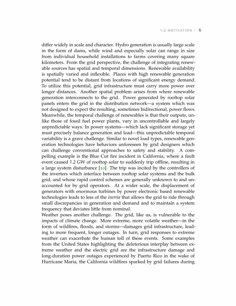


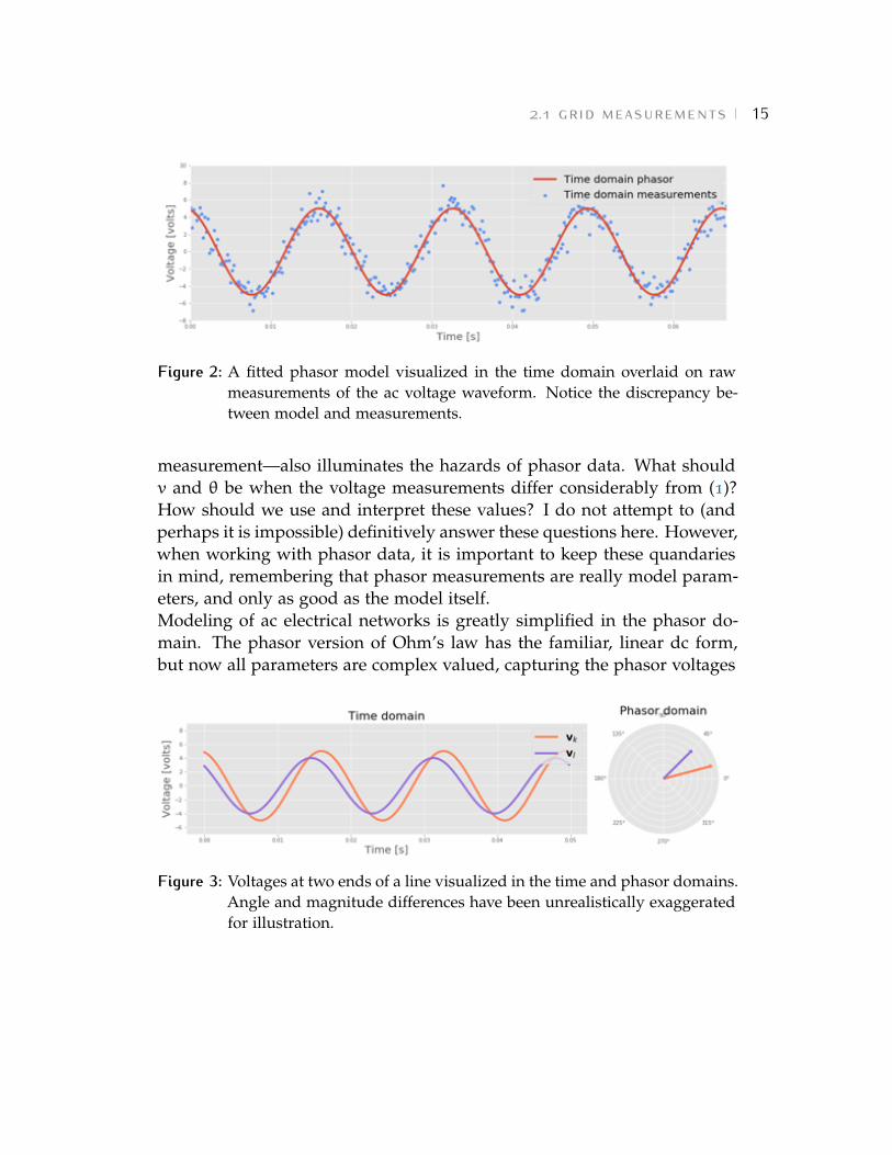


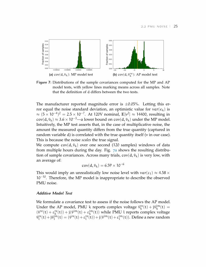


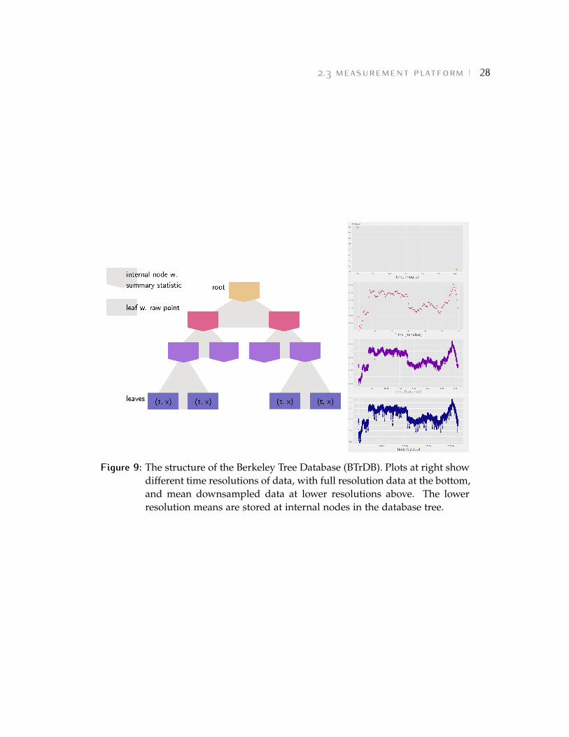


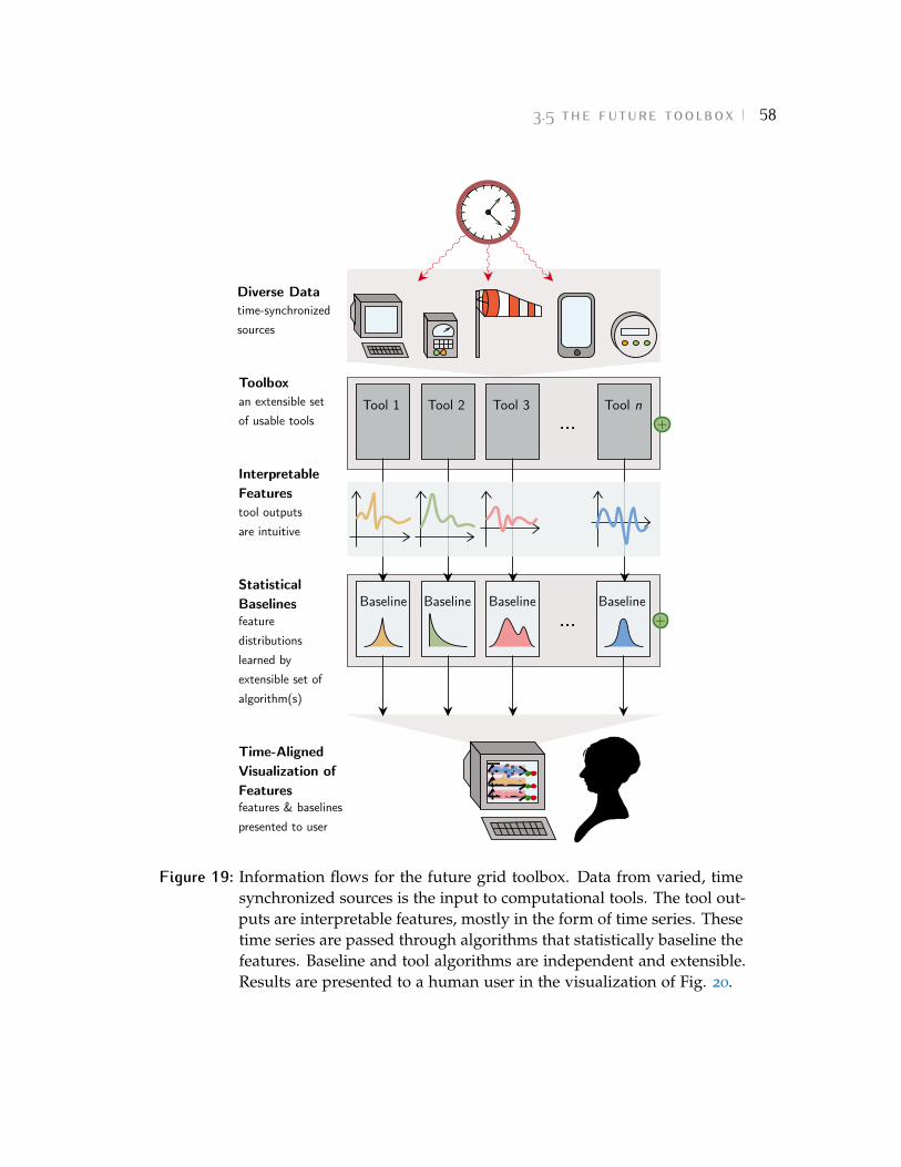


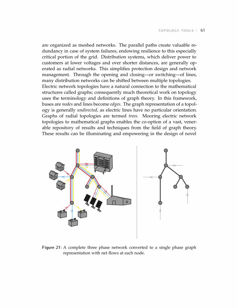


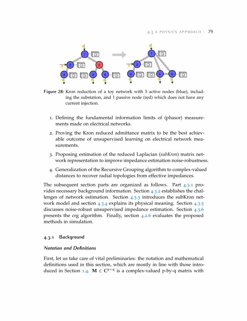


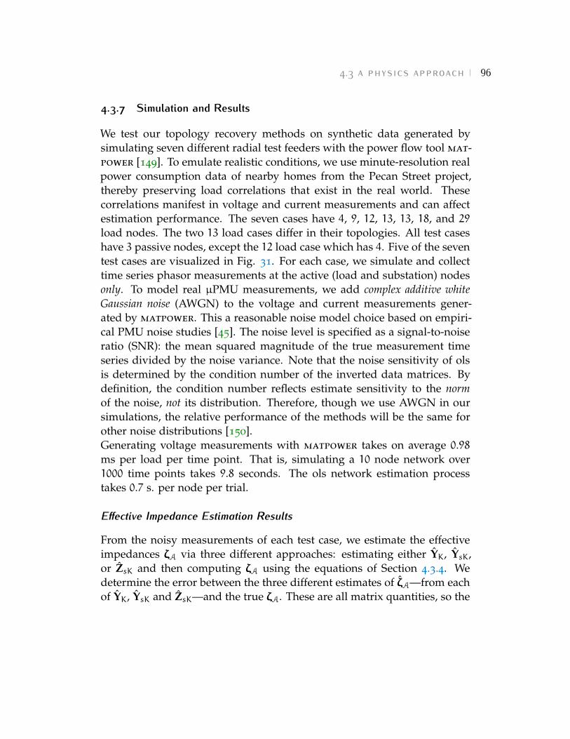


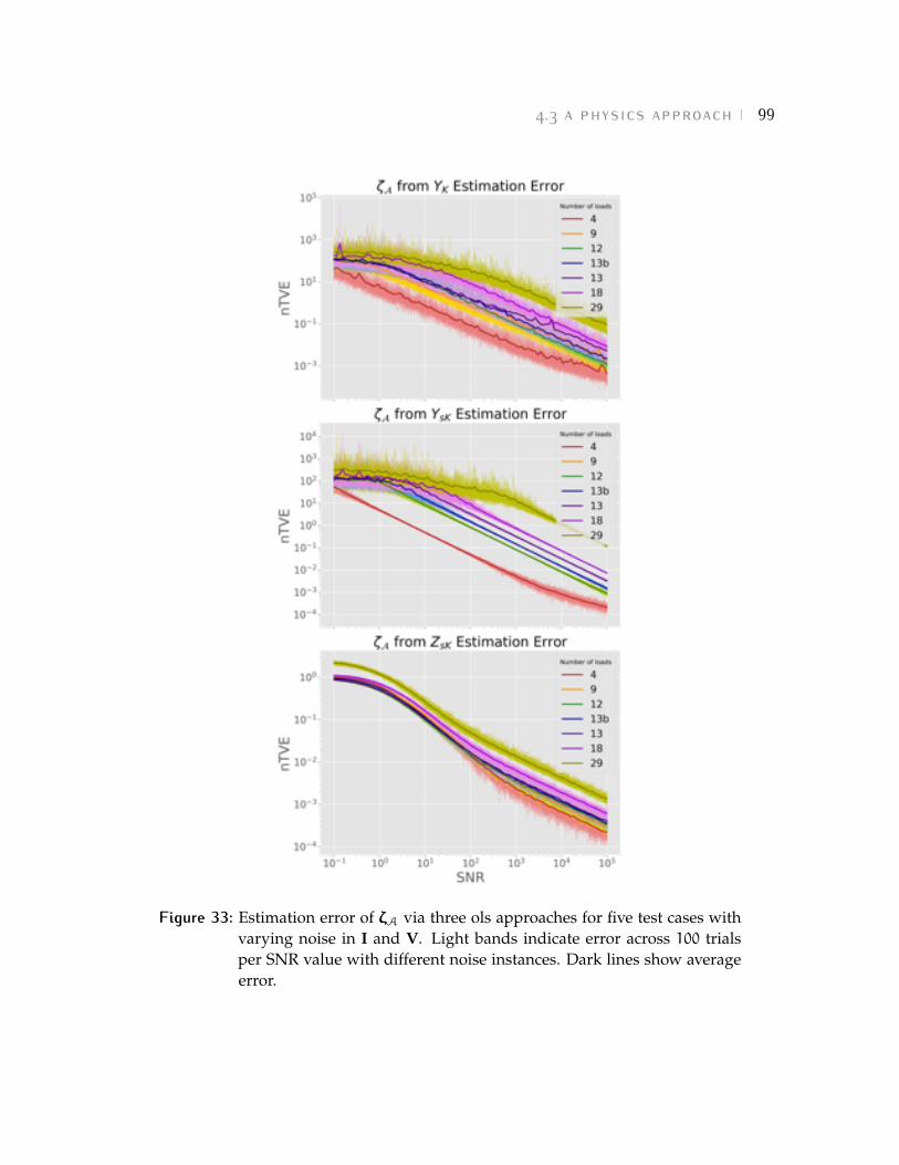


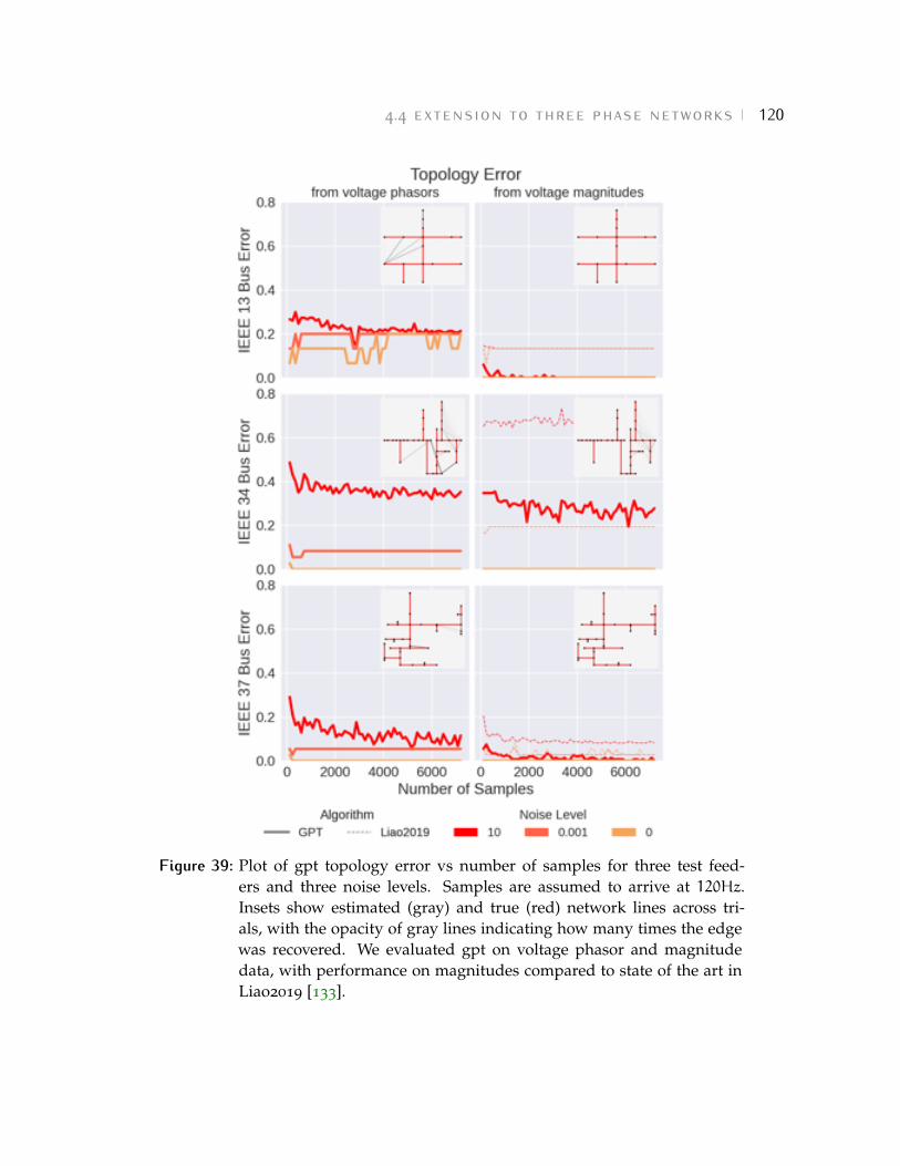


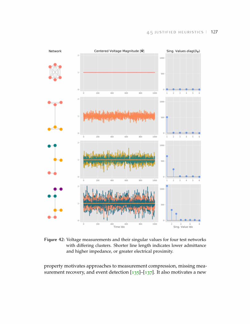


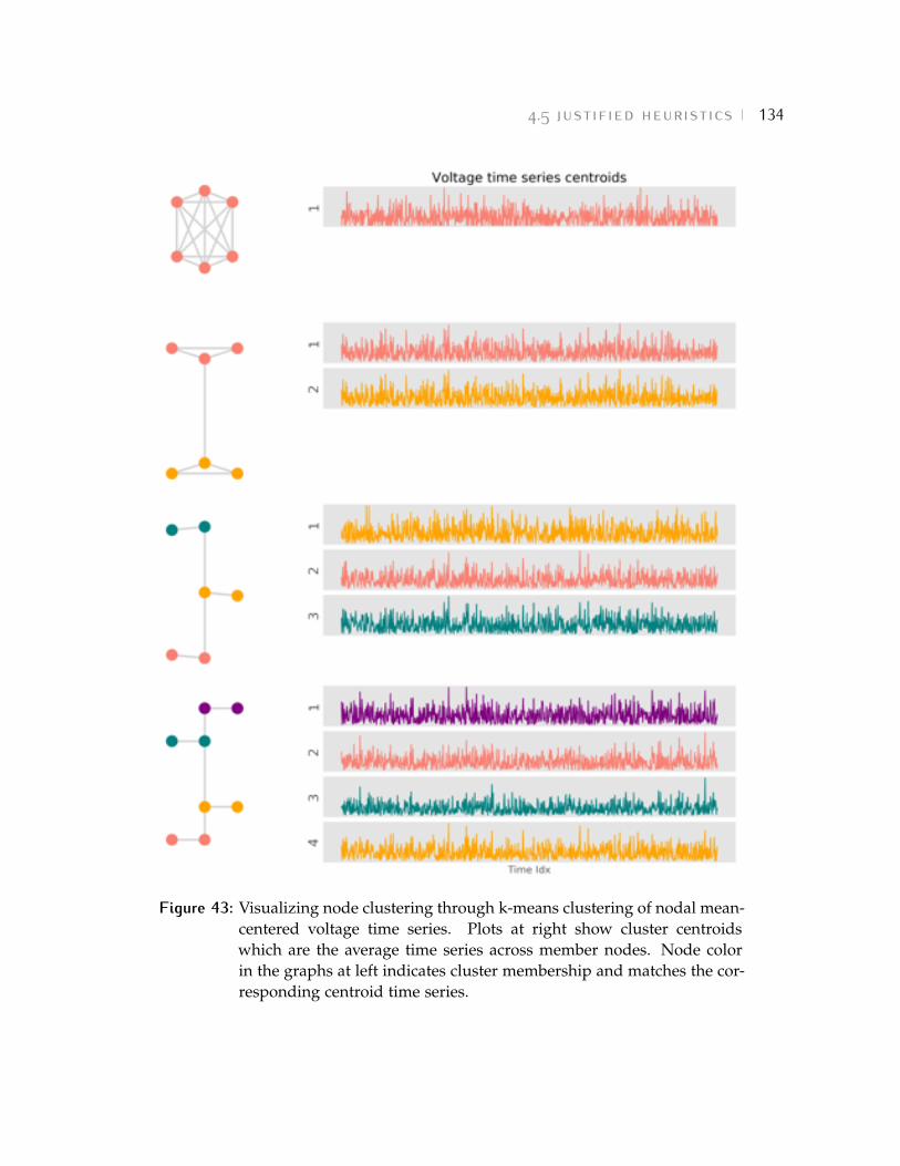
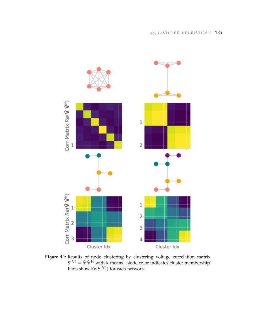
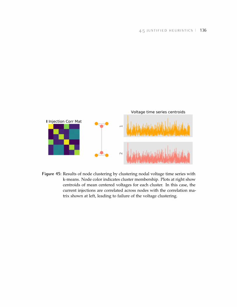


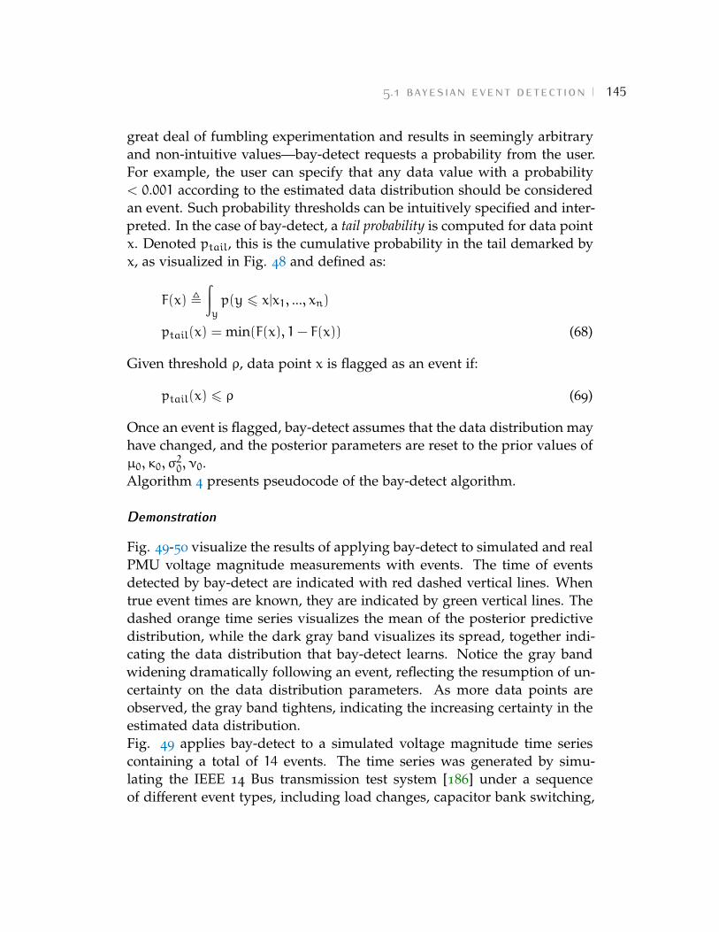


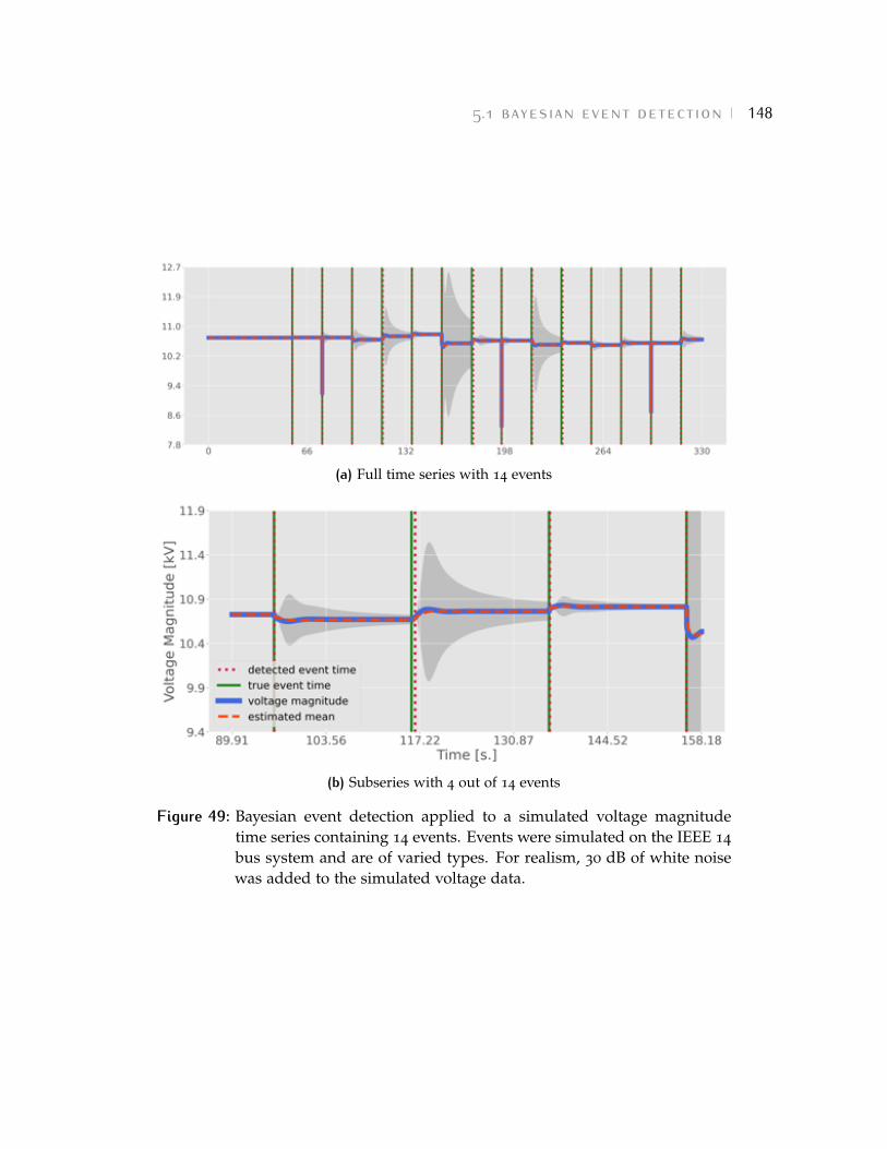
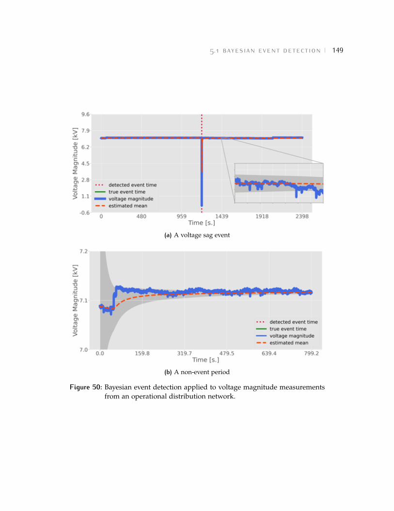


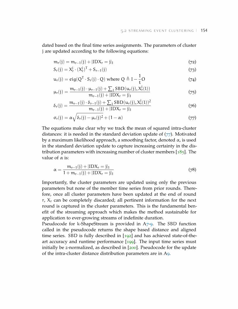


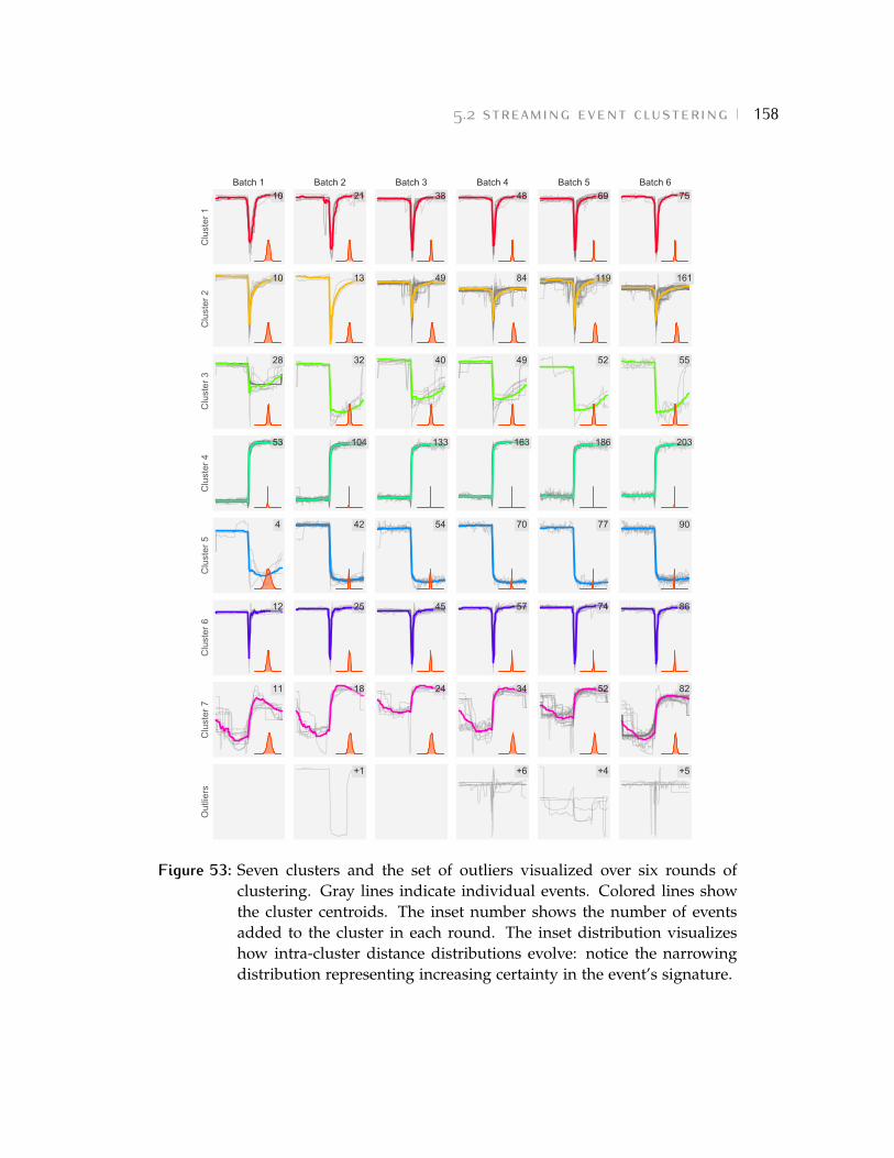


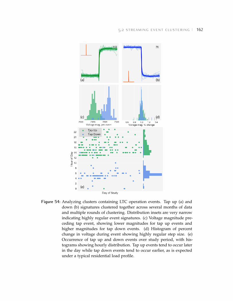


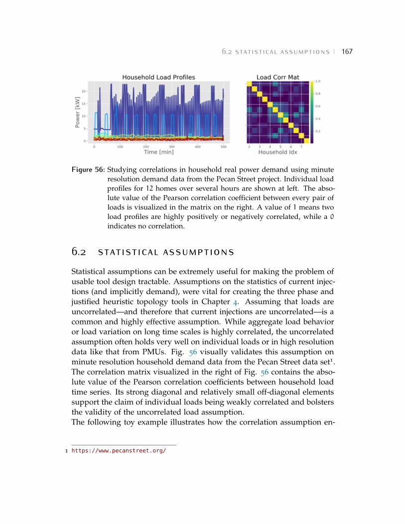


![Wind Power Plant Voltage Stability Evaluation: Preprint produces very accurate phasor measurements, but it also enables synchronized measurements in the same instant [1-9] ... CjX](https://static.documents.pub/doc/80x56/5af553c67f8b9a154c8f8935/wind-power-plant-voltage-stability-evaluation-preprint-produces-very-accurate-phasor.jpg)
