at SciVerse ScienceDirect

Research in Transportation Economics 36 (2012) 19e29

Contents lists available

Research in Transportation Economics

journal homepage: www.elsevier .com/locate /retrec

Applications of transport economics and imperfect competition

David Meunier a,*, Emile Quinet b

aUniversité Paris-Est, Laboratoire Ville Mobilité Transports, UMR T9403 Ecole des Ponts ParisTech INRETS UPEMLV, Franceb PSE, Ecole des Ponts ParisTech, France

a r t i c l e i n f o

Article history:Available online 1 May 2012

Keywords:Imperfect competitionPricingAssessmentProjectMarket imperfectionMarket powerRailCost pass-throughDownstream pricing

* Corresponding author.E-mail address: meunierd@enpc.fr (D. Meunier).

0739-8859/$ e see front matter � 2012 Elsevier Ltd.doi:10.1016/j.retrec.2012.03.010

a b s t r a c t

The great majority of analyses made in transport economics use, explicitly or, more often, implicitly, thecommon assumption of perfect competition. This is the case, for instance, when infrastructure projectsare evaluated using the mere sum of the surpluses of transport users and providers. Even when puttingaside the question of externalities such as noise, safety or environmental quality, the real chain ofeconomic interactions that takes place in transport provision or downstream of transport provision is nottaken into account. Surely enough, describing and simulating this chain could be quite complex.Nevertheless, it is not uninteresting to try to estimate if it does make a big difference or not to make thisapproximation. The paper makes such an attempt for two broad kinds of applications of transporteconomics:Transport pricing: building on a generic formulation of imperfect competition pricing behaviour thatencompasses a broad range of competition situations, and taking the railway case as a benchmark,simulation results give an idea of the order of magnitude of optimal tariff variation when perfectcompetition is assumed as compared to “real” competition situation. These results are completed andsomewhat mitigated by observations on the final welfare impact of this discrepancy.Project assessment: the consequences of imperfect competition situations are analysed, first, for transportprovision, discussing the diverse levels of representation of economic interactions that are used in usualproject assessment. Second, we use both theoretical and heuristic formulations of the interactions thattake place within simple chains of economic actors downstream of transport provision. Besides pure“short sighted” profit maximisation and the base case of perfect competition, the more general imperfectcompetition modelling mentioned above is completed with simple “surplus sharing” behaviours.As a whole, imperfect competition effects seem to be high within the transport sector and should betreated, both for project assessment and for infrastructure pricing. The case is less clear as regardsimperfect competition downstream of transport but still deserves attention. The numerous simulationsand the economic analyses performed lead us to give hints for improving some of the current practices ofeconomic assessment concerning infrastructure pricing and project assessment.

� 2012 Elsevier Ltd. All rights reserved.

1. Introduction

The great majority of transport infrastructure decision-makingrecommendations use, explicitly or more often implicitly, thegeneral assumption of perfect competition. This is the case of themarginal cost pricing principle or, in the case of project appraisal,when infrastructure projects are evaluated using the mere sum ofthe surpluses of transport users and providers. The chain ofeconomic interactions that takes place downstream of transportprovision is generally assumed to be in a classical first best situa-tion, run by perfect competition, with perfect taxes, no externalitiesand constant returns to scale. This assumption is necessary for the

All rights reserved.

validity of the usual partial equilibrium analysis which underliesboth usual pricing doctrines and cost-benefit analyses (see forinstance Lesourne, 1960 quoted by Quinet, 1998 and Quinet &Vickerman, 2004). As soon as these assumptions are not fulfilled,the formulae and criteria become much more complicated. Thispoint is exemplified by a rich literature, reviewed for instance byVickerman (2007).

The sources of imperfection are manifold and each of them isa cause of departure from the usual practices. A first type ofimperfection is related to equity concerns which undermine theusual assumption of optimal distribution obtained by transfersthrough non distorting taxes; for instance Mayeres and Proost(2001) and Mayeres, Proost, Quinet, Schwartz, and Sessa (2001)have taken into account the consequences of imperfect taxes onequity and environmental externalities. Other imperfections are

D. Meunier, E. Quinet / Research in Transportation Economics 36 (2012) 19e2920

linked to the so-called agglomeration externalities, which lead toa lot of recent developments both on the theoretical and on thepractical sides (for instance Graham, 2007). Increasing returns toscale in the whole economy are another source of imperfectionwhich can lead to two different developments; first, along withspatial consideration, these increasing returns to scale are the coreof the new economic geography and have consequences on loca-tions and relocations,with consequences onwelfare calculation (seefor instance Behrens, Gaigné, & Thisse, 2009 for a recent contribu-tion in this field); second, even without spatial consideration,increasing returns to scale induce market imperfections such as theemergence of monopolies or oligopolies leading to departures fromthe competitive assumption and the first best results it implies.

This text considers neither spatial consequences nor agglom-eration externalities as a lot of attention has already been paid tothese effects, both on the theoretical and on the applied sides.

It addresses the consequences of imperfect competition in theeconomy, and this choice is motivated by several reasons; first, ithas not been so extensively addressed; second, it is possible todesign simple models which allow taking a view of the magnitudeof these effects; third, market imperfections of that kind arewidespread, especially in the transport sector; fourth, competitionmay vary a lot among the modes and, if these differences are nottaken into account, it may lead to large distortions between modesand errors in practical decisions.

This text concentrates on two issues, infrastructure pricing andproject assessment. The second section explains the sources andkinds of market imperfection under consideration, and presentshypotheses about firm behaviours. The third section addresses theconsequences of market imperfection on infrastructure pricing. Thefourth section analyses the consequences of market imperfectionson project assessment, again in the transport sector, while the fifthone deals with market imperfections outside the transport sectorand their effects on project assessment.

2. Market imperfection and firm behaviour

2.1. Situations of market imperfection are frequent, especially intransport

Market imperfection can be assessed either from a theoreticalpoint of view through the number of competitors or from anempirical point of view through the Lerner index.

From a theoretical point of view, transport markets are generallycharacterised by the small number of competitors. Let us considerthe rail markets: for long distance passenger traffic, there is ingeneral just one rail operator (RO), the competition is intermodal,the competitor being air transport, and it often happens that thereis just one or a few air competitors on each originedestinationrelation. For medium and short distance passenger traffic, thereare in general just one or very few competing rail operators, and themain competition comes from road transport. Road transport isgenerally regarded as being operated under approximately purecompetition conditions between road hauliers, having no strategicbehaviour1: then, in the case where one RO is competing only withroad transport, everything looks as if the RO were a monopoly. On-track competition is more frequent in freight transport, but hereagain, the competitors are just a few on each single relation.

1 This statement may be challenged by observation of data, though. For instance,data on road haulage costs in France allow to estimate the evolution of proxies ofLerner indexes, which display values that were around 0.4 to 0.5 25 years ago andwent sharply down but are still staying around non-negligible values about 0.15 to0.2 nowadays.

From an empirical point of view, imperfect competition ischaracterised by the fact that the Lerner index (the relative differ-ence between price and marginal cost) is different from zero. Thisfact is well acknowledged for all sectors. Among the most recentstudies let us quote Christopoulou and Vermeulen (2008) whoseinternational survey displays notable mark-up levels in the Euroarea and the US over the period 1981e2004. Still, one may arguethat the deregulation of many sectors may have lead to much lowermark-ups in a more recent period. Bouis (2008) does cover a morerecent period on several OECD countries, and obtains averagemark-ups in the (rounded) range 1.1 to 1.2, which corresponds toLerner indexes of about 0.1 to 0.2; sectoral mark-ups may go up to1.5 and above. The difference between prices and costs is also welldocumented in transport, for instance in the case of air or rail (Ivaldi& Vibes, 2008 for instance).

2.2. How far is the market power exerted?

It is then highly plausible that market power does exist. Theproblem is, then, to estimate to which extent this power is exerted.

What is especially important forour concerns, pricing andprojectassessment, is the firms’ pricing reaction to a variation in costs. Theliterature on this topic has been developing, among other fields, forinternational trade and notably, closer to our transport field, for theautomotive industry. What comes out of the empirical analyses isthat, as Gron and Swenson (2000) tell: “empirical research on costpass-through documents that firms in imperfectly competitivemarkets often pass-through less than 100% of the cost shocks theyexperience”. This is backed also by observations in the transportindustry (Rolin & Sauvant, 2005). Classical results of such studiesdisplay a cost pass-through between 0.5 and 1, that takes severalmonths or even 1 or 2 years to accomplish.Wewill comeback to thispoint in sections 4 and 5. This result is often thoroughly explained bythe classical formulae. When the market power is fully exerted, theLerner index should obey the following well-known formula:

Lhp� cp

¼ �13

(1)

Where 3is the elasticity of the firm (equal to the elasticity of themarket in case of monopoly).

It often happens that these classical formulae do not fit the facts.It is the case for instancewhen, in situation of monopoly, the Lernerindex is lower than the inverse of the market elasticity. There issome evidence that this situation can happen, especially in the caseof transport. DIFFERENT (2008) and Meunier and Quinet (2009)make the case for such situations in France, as well as Clark,Jorgensen, and Pedersen (2009) building on the Norwegian trans-port context. Similarly, there are situations, found for instance inthe results of traffic models, where observed elasticities are lowerthan 1 in absolute value.

These considerations led us then to look for a more generalbehaviour than what we could call “classical profit maximisationbehaviour” or “blunt profit maximisation behaviour” so as tointroduce a theoretical formulation that would be more consistentwith such observations, and that could be backed by economicinterpretations explaining firms’ attitudes, possibly by introducinga broader range of concerns than systematic short-term individualsegment-level profit maximisation (Quinet and Meunier inDIFFERENT (2008)).

We use a general formulation which covers not only the twoextreme competition situations of perfect competition and usualprofit maximisation with price competition, but also mixed atti-tudes where the operator is assumed to aim partly to maximise itsprofit and partly to maximise “market welfare” ie welfare without

D. Meunier, E. Quinet / Research in Transportation Economics 36 (2012) 19e29 21

taking account of externalities, by maximising a combination ofboth according to a proportion s:

F ¼ s*P þ ð1� sÞ*ðSUðpÞ þ PÞ (2)

where P is the operator’s profit and SU(p) its users’ surplus. Thisobjective function encompasses both the perfect competition andrough-welfare behaviour if s ¼ 0 or profit maximisation behaviourif s ¼ 1.

It is easy to derive from this assumption that the price posted bythe firm is such as:

Lhp� cp

¼ �s3

(3)

Where c is the firm’s marginal cost, p its price, 3 its demandprice-elasticity and s a parameter between 0 and 1. It is possible,knowing the costs and prices and elasticities, to calibrate the svalue. If s is lower than unity, there is an indication that the firm’sbehaviour is not the profit maximisation, but the more generalbehaviour corresponding to the maximisation of F. Such a behav-iour may be backed by a variety of reasons:

- When the firm is an historical operator, the persistency ofa welfare maximisation goal, remaining from the old status ofpublic firm, through internal processes or managementmentalities

- The effects of a regulation of prices- Political pressures on price levels, implemented into internalself-regulation

- Strategic attitudes of the firm: considerations of socialacceptability, “lean dog” strategic attitudes, threat of new entryon the market, reputation for other markets (or for furtherdevelopment of the same market), fear of competitionauthorities, .

- A bad knowledge of the market (for instance, overestimation ofactual elasticities), a bounded rationality behaviour

- Uncertainty on the firm’s estimation of demand elasticity,combined with firm’s risk aversion

- The fact that at least on the short-run, marginal costs are verylow, much lower thanwhat stems from the accounting records.

We will adopt this general formulation and see that in thefollowing calibrations, it often happens that the s parameter islower than unity.

3. Infrastructure pricing under transport marketimperfections

In situations of imperfect competition, Optimal InfrastructureCharges (OIC) can be assessed either through algebraic formulaederived from theoretical considerations based on economic anal-ysis or through simulations reckoning based on real situations. Inthe framework of imperfect competition which is the mark ofcompetition in transport, the first approach gets rapidly limited dueto the complexity of mathematical derivations. Very often theycannot be algebraically tractable as soon as situations not toosimple have to be taken into consideration. As a consequence, onlya few very general and generally well-known results can be derivedthrough such a method.

The second approach, the numerical calculations based on realsituations, allows to use the power of computer calculation and totest more varied and complicated situations.2

2 The following text draws on Quinet (2007) and Meunier and Quinet (2009).

Theoretically, nothing prevents such a method to be applied ona large scale, for instance at the country level. The overall modelwould use as entries the cost and demand functions for each routeof each operator, the ICs to be tested on each route, as well as thestructure of the competition (if any) between the operators; theoutputs would be the prices and the traffic volumes of each modeand various other items such as the profits of the firms, consumers’surplus and welfare. In practice, the implementation of this modelis hampered by the lack of data: we have no good knowledge of thecost functions of the operators at the level of each route; we do notknow precisely what the type of competition between the opera-tors is. This draw-back induces to use more simple and crudemethods, restricting the ambitions of the modelling framework.The method which is implemented can be entitled “sensiblesimulation”, and presents the following features:

� It involves a simple network; in the following we use a singleorigin-destination relation one or two modes serving thisrelation.

� The agents are the final consumers, the transport operators(one rail operator, zero or one operator of the other mode) andthe rail infrastructure manager (RIM). The rail operator pays anIC to the infrastructure manager.

� The nature of competition between the operators is typifiedaccording to the considerations developed in the previoussection. One is a monopoly, which aims at reproducing the caseof medium range link, long of about 200e400 km; the other isa duopoly, aiming at reproducing the case of long distancerelation, of about 500e1000 km where rail is in competitionwith air transport. In the first case the rail service is incompetition with road, and, as we assume here that roadoperators are run under perfect competition, they have nostrategic behaviour and the rail operator (RO) behaves asa monopoly. In the second case the rail service is incompetition with an air operator or a few air operators andthe competition between air and rail takes the shape ofa Bertrand competition between two firms supplyingsubstitute services: the Rail Operator (RO) and the AirlineCompany (AC).

� A continuum of possible behaviours for the operators isencompassed, according to the considerations developed in theprevious section, between two extreme cases: the marginalcost pricing corresponding to the behaviour of an operatoraiming at maximising the welfare and the profit maximisingbehaviour.

� The demand function is either a linear one or a logit one.� The cost functions of the operators are linear.� The parameters of the cost and demand functions are notcalibrated on a specific real situation, but set up in order toreproduce typical situations such as: long distance tripscompetition between air and rail or short distance competitionbetween road and rail. The values of the parameters are set inaccordance with the common knowledge of the specialists ofthe field; elasticities are drawn from the results of currenttrafficmodels, costs are drawn fromvarious analyses of the coststructure of operators.

� Other parameters are introduced such as the cost of publicfunds or external costs.

The outputs are the Optimal Infrastructure Charge (OIC), thecorresponding traffic volumes and prices, the profits of the firms(the RIM, the RO and in case of duopoly the AC), the users’ surplusesand the welfare.

The fact that the network and the modelling principles aresimple and do not involve much data allows to make a lot of

Table 1Main data set.

Market structure Link A B C D E F

Monopoly Duopoly

Constant unit parametersRail infrastructure

costb 2.06 2.06 2.13 3.44 5.52 5.21

Environmentalcosts

e1 1 2.25 1.75 3.5 4.5 4e2 4.4 9.9 7.7 15.4 19.8 17.6

Operator’s costs c1 16 13 16 19 24 16c2 55 80 65

Variables describing the current situationOperator’s prices P1 43 43 52 48 59 50

P2 62 102 85Elasticities E11 �0.9 �1 �0.9 �1.5 �1.2 �1.5

E22 �1.7 �1.5 �1.5E12 0.8 2.3 2.5E21 1.5 1.5 1.5

Traffic Q1 0.31 0.26 0.33 0.31 0.24 0.17Q2 0.39 0.45 0.51

Infrastructurecharges

RIC 12.60 12.60 5.8 16.15 20.56 10.28

Table 3Effects of external costs on OIC in the case of profit maximiser operators.

Link Market structure External costs Rail price OIC

e1 e2 p1

B Monopoly 0 0 32.9 0.4B 2.25 9.9 30.9 �2.0E Duopoly 0 0 64.4 20.4

D. Meunier, E. Quinet / Research in Transportation Economics 36 (2012) 19e2922

simulations regarding the shape of the demand function, the valuesof the parameters, the behaviour of the operators, and therefore toby-pass the scarcity of reliable data through exploration of thesensitivity of the results to the parameters.

Six cases are used, and the relevant data set is presented inTable 1. Situations A to C are “monopoly-like” situations ofcompetition between high speed train and motorways for diversetravel distances, so as to represent more or less tough competitionconditions and market shares for rail; in these cases subscripts 1relate to rail and subscripts 2 relate to road. Situations D to F aresituations where high speed train is competing with air transport,again for diverse travel distances so as to represent a range ofcompetition situations and a variety of relative competitiveadvantages for rail; in these cases, subscripts 1 relate to rail andsubscripts 2 relate to air.

From the numerous simulations, we quote and illustrate themore salient features.3

First, as long as there is market power in the downstreammarket, and in absence of Cost of Public Funds (CPF), the OIC arelow, and lower than the marginal infrastructure costs. It is neces-sary to decrease the prices of the operator’s inputs, and the singleinput onwhich the IM can act is the IC. This point is exemplified forinstance in the case of a profit maximiser monopoly, as shown byTable 2:

Table 2Comparison of OIC and marginal infrastructure cost in the case of a profit maximisermonopoly.

Link Costs of public funds Optimalinfrastructure charge

Marginalinfrastructure cost

IM RO 0IC b

C 1 1 �34.2 2.1C 1.3 1 �5.7 2.1C 1.5 1 4.3 2.1

A 1 1 �18.9 2.1A 1.3 1 5.9 2.1A 1.3 1.3 �1.5 2.1

E 4.5 19.8 59.1 14.0

Table 4Consequences of a sub-optimal IC (CPF of the IM ¼ 1.3; CPF of the RO ¼ 1.0; profitmaximiser operators).

Link Marketstatus

Comment IC Welfare Revenues of

IM RO

A Monopoly In this simulation the IC is themarginal cost of infrastructure

2.06 45.1 5.6 5.9

A In this simulation the ICis the OIC

9.0 46.3 2.9 7.6

D Duopoly In this simulation the IC is themarginal cost of infrastructure

3.4 46.5 0.1 8.9

D In this simulation the ICis the optimal one

2.0 46.7 �0.9 9.7

The direction of Optimal Infrastructure Charge (OIC) variationsis normal from a theoretical point of view. The surprising point is

3 More details on the simulation process, calculations and data can be found inMeunier and Quinet (2009) and in DIFFERENT (2008).

the high distance between marginal cost and OIC. It is not a matterof small correction, but of magnitude. It even happens that in somecases, the charge should become a subsidy. This table shows alsothat the gap highly depends on the value of the CPF. OIC increaseswith the CPF of the IM. It appears that in the cases under review,OIC is equal to the marginal infrastructure cost for values of CPFaround 1.3 to 1.5 for the IM and 1.0 for the operator. When both CPFof the IM and of the operator are equal, optimal IC increases withthese CPF and becomes equal to the marginal cost of infrastructurewhen they are infinite.

Second, taking into account the external costs increases the IC ifthe mode is less environmental friendly than its competitor, anddecreases it in the reverse situationwhich is usually the case for railvis-à-vis air or road transport. Table 3 shows examples of theseeffects which go in the expected direction. But it appears that theintensity of the effect is rather low. In the range of values consid-ered, external costs tend to have observable but lower impacts onprices and optimal charges, as compared to the impact of CPF. Andunlike the current doctrine which would lead to add the netexternal cost to the IC, optimal pricing does transmit only a fractionof external costs in the IC.

Another striking fact is the change in welfare induced bychanges in the IC. It stems from Table 4 below that, as long as the ICare not “too” different from the OIC, the changes in welfare aresmall and that the effect of a sub-optimal IC bears mainly on thecomponents of welfare: revenues of the IM and the operator’srevenues and consumer surplus.

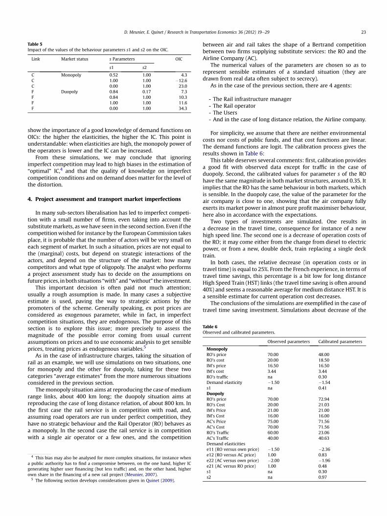
Another important point is to properly assess the behaviours ofthe firms, expressed by the values of the parameters s. In otherwords, does the quality of representation of imperfect competitionmatter much on OIC, and therefore on the distortion introduced byPerfect Competition Assumption (PCA) relatively to OIC? As shownin the Table 5, the behaviour of the rail’s competitor (the value ofs2) does not impact too much the optimal solution, while largechanges from the initial value s1 lead to important differencesbetween the calculated IC and the optimal one.

Lastly, does the quality of knowledge on demand impact muchon OIC levels, and therefore on the gap between OIC and the resultsof PCA pricing? A last series of simulations, not reproduced here,

Table 5Impact of the values of the behaviour parameters s1 and s2 on the OIC.

Link Market status s Parameters OIC

s1 s2

C Monopoly 0.52 1.00 4.3C 1.00 1.00 �12.6C 0.00 1.00 23.0F Duopoly 0.84 0.17 7.3F 0.84 1.00 10.3F 1.00 1.00 11.6F 0.00 1.00 34.3

Table 6Observed and calibrated parameters.

Observed parameters Calibrated parameters

MonopolyRO’s price 70.00 48.00RO’s cost 20.00 18.50IM’s price 16.50 16.50IM’s cost 3.44 3.44RO’s traffic na 0.30Demand elasticity �1.50 �1.54s1 na 0.41DuopolyRO’s price 70.00 72.94RO’s Cost 20.00 21.03IM’s Price 21.00 21.00IM’s Cost 16.00 16.00AC’s Price 75.00 71.56AC’s Cost 70.00 71.56RO’s Traffic 60.00 23.06AC’s Traffic 40.00 40.63

D. Meunier, E. Quinet / Research in Transportation Economics 36 (2012) 19e29 23

show the importance of a good knowledge of demand functions onOICs: the higher the elasticities, the higher the IC. This point isunderstandable: when elasticities are high, the monopoly power ofthe operators is lower and the IC can be increased.

From these simulations, we may conclude that ignoringimperfect competition may lead to high biases in the estimation of“optimal” IC,4 and that the quality of knowledge on imperfectcompetition conditions and on demand does matter for the level ofthe distortion.

4. Project assessment and transport market imperfections

In many sub-sectors liberalisation has led to imperfect competi-tion with a small number of firms, even taking into account thesubstitutemarkets, aswehave seen in the second section. Even if thecompetitionwished for instance by the European Commission takesplace, it is probable that the number of actors will be very small oneach segment of market. In such a situation, prices are not equal tothe (marginal) costs, but depend on strategic interactions of theactors, and depend on the structure of the market: how manycompetitors and what type of oligopoly. The analyst who performsa project assessment study has to decide on the assumptions onfutureprices, inboth situations “with” and “without” the investment.

This important decision is often paid not much attention;usually a rough assumption is made. In many cases a subjectiveestimate is used, paving the way to strategic actions by thepromoters of the scheme. Generally speaking, ex post prices areconsidered as exogenous parameter, while in fact, in imperfectcompetition situations, they are endogenous. The purpose of thissection is to explore this issue; more precisely to assess themagnitude of the possible error coming from usual currentassumptions on prices and to use economic analysis to get sensibleprices, treating prices as endogenous variables.5

As in the case of infrastructure charges, taking the situation ofrail as an example, we will use simulations on two situations, onefor monopoly and the other for duopoly, taking for these twocategories “average estimates” from the more numerous situationsconsidered in the previous section.

Themonopoly situation aims at reproducing the case of mediumrange links, about 400 km long; the duopoly situation aims atreproducing the case of long distance relation, of about 800 km. Inthe first case the rail service is in competition with road, and,assuming road operators are run under perfect competition, theyhave no strategic behaviour and the Rail Operator (RO) behaves asa monopoly. In the second case the rail service is in competitionwith a single air operator or a few ones, and the competition

4 This bias may also be analysed for more complex situations, for instance whena public authority has to find a compromise between, on the one hand, higher ICgenerating higher user financing (but less traffic) and, on the other hand, higherown share in the financing of a new rail project (Meunier, 2007).

5 The following section develops considerations given in Quinet (2009).

between air and rail takes the shape of a Bertrand competitionbetween two firms supplying substitute services: the RO and theAirline Company (AC).

The numerical values of the parameters are chosen so as torepresent sensible estimates of a standard situation (they aredrawn from real data often subject to secrecy).

As in the case of the previous section, there are 4 agents:

- The Rail infrastructure manager- The Rail operator- The Users- And in the case of long distance relation, the Airline company.

For simplicity, we assume that there are neither environmentalcosts nor costs of public funds, and that cost functions are linear.The demand functions are logit. The calibration process gives theresults shown in Table 6:

This table deserves several comments: first, calibration providesa good fit with observed data except for traffic in the case ofduopoly. Second, the calibrated values for parameter s of the ROhave the samemagnitude in bothmarket structures, around 0.35. Itimplies that the RO has the same behaviour in both markets, whichis sensible. In the duopoly case, the value of the parameter for theair company is close to one, showing that the air company fullyexerts its market power in almost pure profit maximiser behaviour,here also in accordance with the expectations.

Two types of investments are simulated. One results ina decrease in the travel time, consequence for instance of a newhigh speed line. The second one is a decrease of operation costs ofthe RO; it may come either from the change from diesel to electricpower, or from a new, double deck, train replacing a single decktrain.

In both cases, the relative decrease (in operation costs or intravel time) is equal to 25%. From the French experience, in terms oftravel time savings, this percentage is a bit low for long distanceHigh Speed Train (HST) links (the travel time saving is often around40%) and seems a reasonable average for medium distance HST. It isa sensible estimate for current operation cost decreases.

The conclusions of the simulations are exemplified in the case oftravel time saving investment. Simulations about decrease of the

Demand elasticitiese11 (RO versus own price) �1.50 �2.36e12 (RO versus AC price) 1.00 0.83e22 (AC versus own price) �2.00 �1.96e21 (AC versus RO price) 1.00 0.48s1 na 0.30s2 na 0.97

D. Meunier, E. Quinet / Research in Transportation Economics 36 (2012) 19e2924

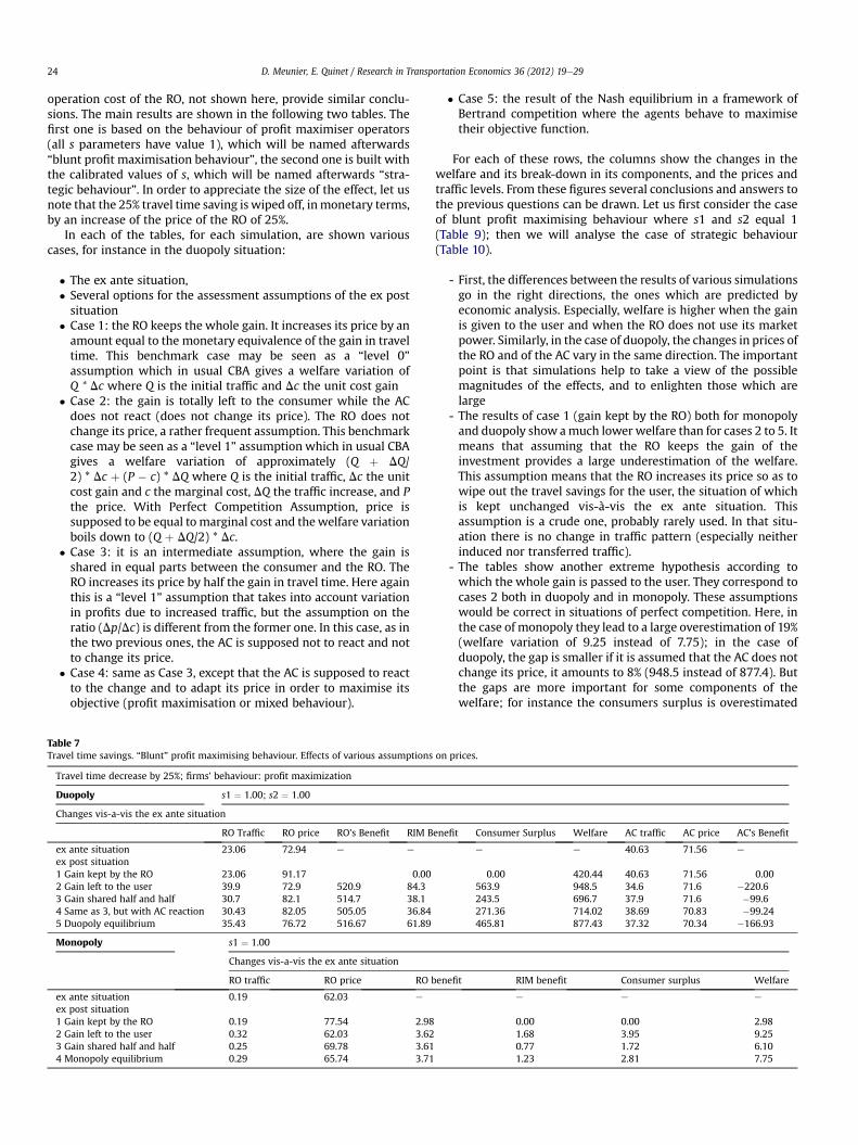
operation cost of the RO, not shown here, provide similar conclu-sions. The main results are shown in the following two tables. Thefirst one is based on the behaviour of profit maximiser operators(all s parameters have value 1), which will be named afterwards“blunt profit maximisation behaviour”, the second one is built withthe calibrated values of s, which will be named afterwards “stra-tegic behaviour”. In order to appreciate the size of the effect, let usnote that the 25% travel time saving is wiped off, inmonetary terms,by an increase of the price of the RO of 25%.

In each of the tables, for each simulation, are shown variouscases, for instance in the duopoly situation:

� The ex ante situation,� Several options for the assessment assumptions of the ex postsituation

� Case 1: the RO keeps the whole gain. It increases its price by anamount equal to the monetary equivalence of the gain in traveltime. This benchmark case may be seen as a “level 0”assumption which in usual CBA gives a welfare variation ofQ * Dc where Q is the initial traffic and Dc the unit cost gain

� Case 2: the gain is totally left to the consumer while the ACdoes not react (does not change its price). The RO does notchange its price, a rather frequent assumption. This benchmarkcase may be seen as a “level 1” assumption which in usual CBAgives a welfare variation of approximately (Q þ DQ/2) * Dc þ (P � c) * DQ where Q is the initial traffic, Dc the unitcost gain and c the marginal cost, DQ the traffic increase, and Pthe price. With Perfect Competition Assumption, price issupposed to be equal to marginal cost and thewelfare variationboils down to (Q þ DQ/2) * Dc.

� Case 3: it is an intermediate assumption, where the gain isshared in equal parts between the consumer and the RO. TheRO increases its price by half the gain in travel time. Here againthis is a “level 1” assumption that takes into account variationin profits due to increased traffic, but the assumption on theratio (Dp/Dc) is different from the former one. In this case, as inthe two previous ones, the AC is supposed not to react and notto change its price.

� Case 4: same as Case 3, except that the AC is supposed to reactto the change and to adapt its price in order to maximise itsobjective (profit maximisation or mixed behaviour).

Table 7Travel time savings. “Blunt” profit maximising behaviour. Effects of various assumptions

Travel time decrease by 25%; firms’ behaviour: profit maximization

Duopoly s1 ¼ 1.00; s2 ¼ 1.00

Changes vis-a-vis the ex ante situation

RO Traffic RO price RO’s Benefit RIM B

ex ante situation 23.06 72.94 e e

ex post situation1 Gain kept by the RO 23.06 91.17 0.002 Gain left to the user 39.9 72.9 520.9 84.33 Gain shared half and half 30.7 82.1 514.7 38.14 Same as 3, but with AC reaction 30.43 82.05 505.05 36.845 Duopoly equilibrium 35.43 76.72 516.67 61.89

Monopoly s1 ¼ 1.00

Changes vis-a-vis the ex ante situation

RO traffic RO price RO b

ex ante situation 0.19 62.03 e

ex post situation1 Gain kept by the RO 0.19 77.54 2.982 Gain left to the user 0.32 62.03 3.623 Gain shared half and half 0.25 69.78 3.614 Monopoly equilibrium 0.29 65.74 3.71

� Case 5: the result of the Nash equilibrium in a framework ofBertrand competition where the agents behave to maximisetheir objective function.

For each of these rows, the columns show the changes in thewelfare and its break-down in its components, and the prices andtraffic levels. From these figures several conclusions and answers tothe previous questions can be drawn. Let us first consider the caseof blunt profit maximising behaviour where s1 and s2 equal 1(Table 9); then we will analyse the case of strategic behaviour(Table 10).

- First, the differences between the results of various simulationsgo in the right directions, the ones which are predicted byeconomic analysis. Especially, welfare is higher when the gainis given to the user and when the RO does not use its marketpower. Similarly, in the case of duopoly, the changes in prices ofthe RO and of the AC vary in the same direction. The importantpoint is that simulations help to take a view of the possiblemagnitudes of the effects, and to enlighten those which arelarge

- The results of case 1 (gain kept by the RO) both for monopolyand duopoly show amuch lower welfare than for cases 2 to 5. Itmeans that assuming that the RO keeps the gain of theinvestment provides a large underestimation of the welfare.This assumption means that the RO increases its price so as towipe out the travel savings for the user, the situation of whichis kept unchanged vis-à-vis the ex ante situation. Thisassumption is a crude one, probably rarely used. In that situ-ation there is no change in traffic pattern (especially neitherinduced nor transferred traffic).

- The tables show another extreme hypothesis according towhich the whole gain is passed to the user. They correspond tocases 2 both in duopoly and in monopoly. These assumptionswould be correct in situations of perfect competition. Here, inthe case of monopoly they lead to a large overestimation of 19%(welfare variation of 9.25 instead of 7.75); in the case ofduopoly, the gap is smaller if it is assumed that the AC does notchange its price, it amounts to 8% (948.5 instead of 877.4). Butthe gaps are more important for some components of thewelfare; for instance the consumers surplus is overestimated

on prices.

enefit Consumer Surplus Welfare AC traffic AC price AC’s Benefit

e e 40.63 71.56 e

0.00 420.44 40.63 71.56 0.00563.9 948.5 34.6 71.6 �220.6243.5 696.7 37.9 71.6 �99.6271.36 714.02 38.69 70.83 �99.24465.81 877.43 37.32 70.34 �166.93

enefit RIM benefit Consumer surplus Welfare

e e e

0.00 0.00 2.981.68 3.95 9.250.77 1.72 6.101.23 2.81 7.75

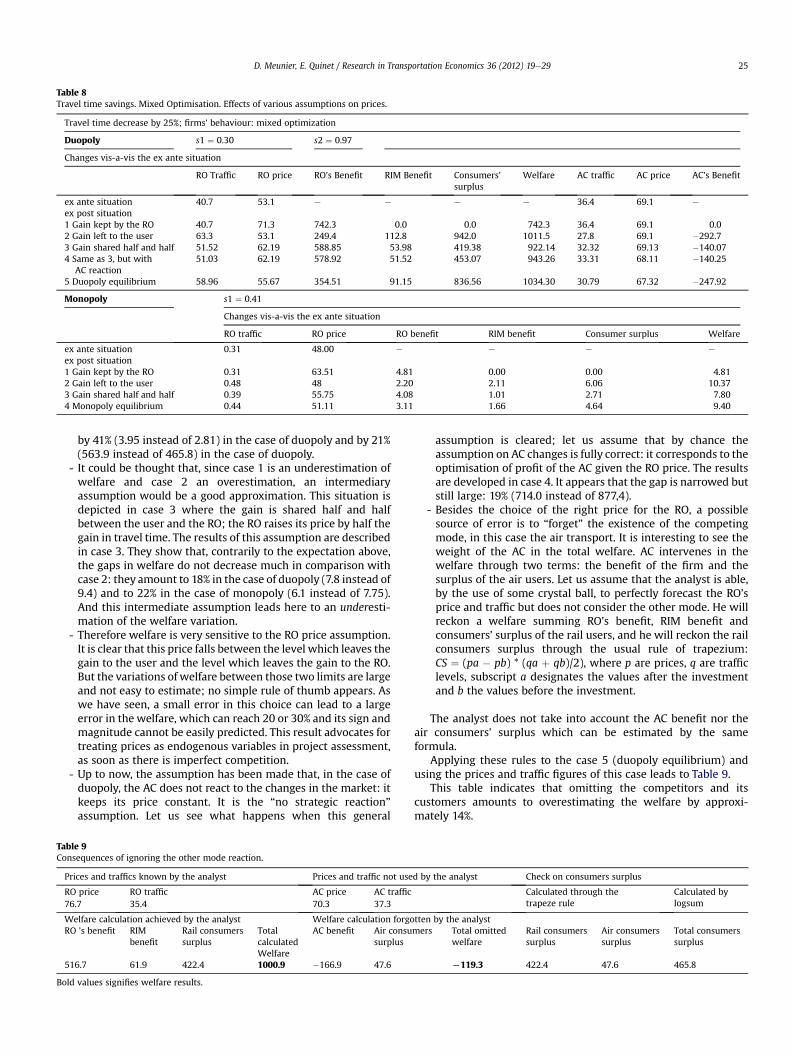
Table 8Travel time savings. Mixed Optimisation. Effects of various assumptions on prices.

Travel time decrease by 25%; firms’ behaviour: mixed optimization

Duopoly s1 ¼ 0.30 s2 ¼ 0.97

Changes vis-a-vis the ex ante situation

RO Traffic RO price RO’s Benefit RIM Benefit Consumers’surplus

Welfare AC traffic AC price AC’s Benefit

ex ante situation 40.7 53.1 e e e e 36.4 69.1 e

ex post situation1 Gain kept by the RO 40.7 71.3 742.3 0.0 0.0 742.3 36.4 69.1 0.02 Gain left to the user 63.3 53.1 249.4 112.8 942.0 1011.5 27.8 69.1 �292.73 Gain shared half and half 51.52 62.19 588.85 53.98 419.38 922.14 32.32 69.13 �140.074 Same as 3, but with

AC reaction51.03 62.19 578.92 51.52 453.07 943.26 33.31 68.11 �140.25

5 Duopoly equilibrium 58.96 55.67 354.51 91.15 836.56 1034.30 30.79 67.32 �247.92

Monopoly s1 ¼ 0.41

Changes vis-a-vis the ex ante situation

RO traffic RO price RO benefit RIM benefit Consumer surplus Welfare

ex ante situation 0.31 48.00 e e e e

ex post situation1 Gain kept by the RO 0.31 63.51 4.81 0.00 0.00 4.812 Gain left to the user 0.48 48 2.20 2.11 6.06 10.373 Gain shared half and half 0.39 55.75 4.08 1.01 2.71 7.804 Monopoly equilibrium 0.44 51.11 3.11 1.66 4.64 9.40

D. Meunier, E. Quinet / Research in Transportation Economics 36 (2012) 19e29 25

by 41% (3.95 instead of 2.81) in the case of duopoly and by 21%(563.9 instead of 465.8) in the case of duopoly.

- It could be thought that, since case 1 is an underestimation ofwelfare and case 2 an overestimation, an intermediaryassumption would be a good approximation. This situation isdepicted in case 3 where the gain is shared half and halfbetween the user and the RO; the RO raises its price by half thegain in travel time. The results of this assumption are describedin case 3. They show that, contrarily to the expectation above,the gaps in welfare do not decrease much in comparison withcase 2: they amount to 18% in the case of duopoly (7.8 instead of9.4) and to 22% in the case of monopoly (6.1 instead of 7.75).And this intermediate assumption leads here to an underesti-mation of the welfare variation.

- Therefore welfare is very sensitive to the RO price assumption.It is clear that this price falls between the level which leaves thegain to the user and the level which leaves the gain to the RO.But the variations of welfare between those two limits are largeand not easy to estimate; no simple rule of thumb appears. Aswe have seen, a small error in this choice can lead to a largeerror in the welfare, which can reach 20 or 30% and its sign andmagnitude cannot be easily predicted. This result advocates fortreating prices as endogenous variables in project assessment,as soon as there is imperfect competition.

- Up to now, the assumption has been made that, in the case ofduopoly, the AC does not react to the changes in the market: itkeeps its price constant. It is the “no strategic reaction”assumption. Let us see what happens when this general

Table 9Consequences of ignoring the other mode reaction.

Prices and traffics known by the analyst Prices and traffic not use

RO price RO traffic AC price AC traffic76.7 35.4 70.3 37.3

Welfare calculation achieved by the analyst Welfare calculation forgoRO ’s benefit RIM

benefitRail consumerssurplus

TotalcalculatedWelfare

AC benefit Air consusurplus

516.7 61.9 422.4 1000.9 �166.9 47.6

Bold values signifies welfare results.

assumption is cleared; let us assume that by chance theassumption on AC changes is fully correct: it corresponds to theoptimisation of profit of the AC given the RO price. The resultsare developed in case 4. It appears that the gap is narrowed butstill large: 19% (714.0 instead of 877,4).

- Besides the choice of the right price for the RO, a possiblesource of error is to “forget” the existence of the competingmode, in this case the air transport. It is interesting to see theweight of the AC in the total welfare. AC intervenes in thewelfare through two terms: the benefit of the firm and thesurplus of the air users. Let us assume that the analyst is able,by the use of some crystal ball, to perfectly forecast the RO’sprice and traffic but does not consider the other mode. He willreckon a welfare summing RO’s benefit, RIM benefit andconsumers’ surplus of the rail users, and he will reckon the railconsumers surplus through the usual rule of trapezium:CS ¼ (pa � pb) * (qa þ qb)/2), where p are prices, q are trafficlevels, subscript a designates the values after the investmentand b the values before the investment.

The analyst does not take into account the AC benefit nor theair consumers’ surplus which can be estimated by the sameformula.

Applying these rules to the case 5 (duopoly equilibrium) andusing the prices and traffic figures of this case leads to Table 9.

This table indicates that omitting the competitors and itscustomers amounts to overestimating the welfare by approxi-mately 14%.

d by the analyst Check on consumers surplus

Calculated through thetrapeze rule

Calculated bylogsum

tten by the analystmers Total omitted

welfareRail consumerssurplus

Air consumerssurplus

Total consumerssurplus

L119.3 422.4 47.6 465.8

Table 10Effects of a change in infrastructure charge.

Travel time decrease 25%; firms’ behaviours : profit maximisation

Duopoly s1 ¼ 1; s2 ¼ 1

Changes vis-a-vis the ex ante situation

RO’sbenefit

AC’sbenefit

RIMbenefit

Consumersurplus

Welfare IMprice

IM margcost

ROprice

ACprice

ROtraffic

ACtraffic

ex ante situation 21.0 16.0 72.9 71.6 23.1 40.6ex post situationDuopoly equilibrium,

half the gain is given to the IM231.1 �79.3 293.4 215.6 660.8 25.6 16.0 83.7 71.0 28.9 39.1

Duopoly Equilibrium 516.7 �166.9 61.9 465.8 877.4 21.0 16.0 76.7 70.3 35.4 37.3

Monopoly s1 ¼ 1

Changes vis-a-vis the ex ante situation

RO benefit RIM benefit Consumer surplus Welfare IM price IM marg cost RO price RO traffic

ex ante situation 16.2 3.5 62.0 0.2ex post situationMonopoly equilibrium,

half the gain is given to the IM1.7 2.4 1.3 5.4 23.9 3.5 71.5 0.2

Monopoly equilibrium 3.7 1.2 2.8 7.8 16.2 3.5 65.7 0.3

Bold values signifies welfare results.

D. Meunier, E. Quinet / Research in Transportation Economics 36 (2012) 19e2926

This overestimation adds to the error coming from a wrongchoice of the price and traffic of the RO; as we have seen from theprevious considerations, this error can be either an over or anunderestimation, the magnitude of which can reach around 20%.

Tables 7 and 8 show also that the forecasted traffic is highlysensitive to the assumption on prices. Detailed results not shown inTable 9 are similar: in case 2, where the saving is entirely passed tothe user e a frequent assumption which amounts to forgetting thestrategic reactions due to imperfect competition- the error is anoverestimation of rail traffic by 13%, a non-negligible figure. Thiskind of estimation bias may contribute to the explanation of thehigh rail traffic overestimation observed by Flyvbjerg (Flyvbjerg,Skamris Holm, & Buhl, 2006).

Another current practice is to pass a part of the benefits to theInfrastructure Manager which is in charge of infrastructureinvestments and, in many countries, is asked to cover its costs by itsown. It is often implicitly considered that sharing the profitbetween the RO and the IM has no consequence on the welfare andwill not induce strategic consequences on the behaviour of thefirms. The following simulations show that on the contrary, tryingto share the pie has tremendous consequences when the infra-structure charge increase is proportional to the unit gain.

In these simulations the IM increases its price by half the savingper user (in the table above, it increases its price by half the traveltime saving), while the marginal infrastructure cost is unchanged.These values are in accordance with the usual practice which tendsto increase the rate of profit for new lines in order to fund a part ofthe investment. When the IM raises its price, it looses a part of thetraffic. The calculation of its revenue should take into account theimpact of its pricing attitude on the RO’s price and on the traffic.

The effect is important also on the welfare, which gets lower by25% in the case of duopoly (660.8 instead of 877.4) and by 30% inthe case of monopoly (5.4 instead of 7.8). This point prompts us tomake a link with the previous section about optimal pricing, and tocheck how high the cost of public funds should be to justify such anincrease. It is easy to check that it would happen for a CPF such that:

- In the case of duopoly: CPF ¼ 1.93- In the case of monopoly: CPF ¼ 3.

In the present numerical simulations these values largely exceedthe current values of CPF, which, as seen in the previous section, liearound 1.2 to 1.5.

This result advocates for a special attention to the infrastructurecharges and to how they are linked to the gains provided by theinvestment.

All these results are confirmed by the simulations on operationcost savings. The differences are milder since the cost saving ratioused, 25% of the present cost, amounts to a smaller absolute valueof price: 7% instead of 25%.

If now we get a look at the results in the hypothesis of strategicbehaviour, where the s parameters are endogenous, we find milderresults in each case, the gaps between the various hypotheses aresmaller. It is not surprising to see that the hypothesis of a gainpassed to the user and consequently no change in the price providesa welfare very close to the hypothesis of market equilibrium in thiscontext of strategic behaviour: in fact, the blunt profit behaviourfollowed by the firms is intermediate between profit maximisingand (an imperfect version of) welfaremaximising. This result pointsout the importance of precisely knowing the behaviour of the firmsin order to make the proper assumptions about prices.

5. Project assessment and downstream market imperfections

Usual CBA for transport infrastructure projects takes intoaccount surpluses of (all or part) transport users, transportproviders and infrastructure managers, but does not take intoaccount what takes place downstream of transport. For instance,the freight transported is destined to a factory, which will benefitfrom the project by means of economies of time or cost for thistransport. But this benefit may be passed-through, fully or partly, tothe firms that are the factory’s clients, which may in turn pass itthrough downstream.

Thus, usual CBA makes the implicit assumption that the initialtransportbenefit is simplydispatched throughthechainof interactionsdownstream of transport, in a null-sum game; or, at least, that thisassumption is an approximation that has very minor consequences.This assumption is correct in perfect markets (Dodgson, 1973; Jara-Diaz, 1986); but is it the case in practice? Among other authors,Venables and Gasiorek (1999) analysed this question and concludedthat the extent of any underestimation or overestimationwill dependon the degree of variation between price and marginal cost and theelasticity of demand for the activity. The order of magnitude ofunderestimation they obtained for some industries was found to bebetween10%and40%,butoverestimationmighthappen inother cases.

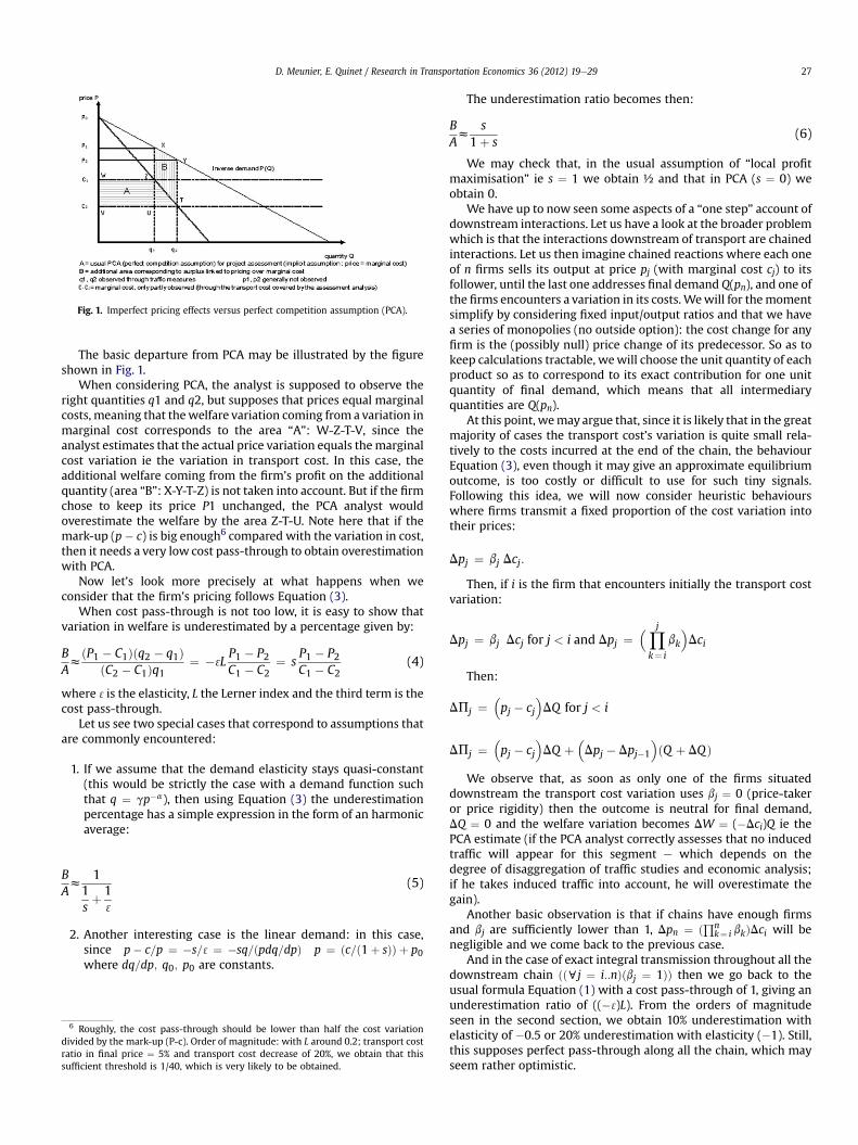
Fig. 1. Imperfect pricing effects versus perfect competition assumption (PCA).

D. Meunier, E. Quinet / Research in Transportation Economics 36 (2012) 19e29 27

The basic departure from PCA may be illustrated by the figureshown in Fig. 1.

When considering PCA, the analyst is supposed to observe theright quantities q1 and q2, but supposes that prices equal marginalcosts, meaning that thewelfare variation coming from a variation inmarginal cost corresponds to the area “A”: W-Z-T-V, since theanalyst estimates that the actual price variation equals themarginalcost variation ie the variation in transport cost. In this case, theadditional welfare coming from the firm’s profit on the additionalquantity (area “B”: X-Y-T-Z) is not taken into account. But if the firmchose to keep its price P1 unchanged, the PCA analyst wouldoverestimate the welfare by the area Z-T-U. Note here that if themark-up (p� c) is big enough6 compared with the variation in cost,then it needs a very low cost pass-through to obtain overestimationwith PCA.

Now let’s look more precisely at what happens when weconsider that the firm’s pricing follows Equation (3).

When cost pass-through is not too low, it is easy to show thatvariation in welfare is underestimated by a percentage given by:

BAz

ðP1 � C1Þðq2 � q1ÞðC2 � C1Þq1

¼ � 3LP1 � P2C1 � C2

¼ sP1 � P2C1 � C2

(4)

where 3is the elasticity, L the Lerner index and the third term is thecost pass-through.

Let us see two special cases that correspond to assumptions thatare commonly encountered:

1. If we assume that the demand elasticity stays quasi-constant(this would be strictly the case with a demand function suchthat q ¼ gp�a), then using Equation (3) the underestimationpercentage has a simple expression in the form of an harmonicaverage:

BAz

11sþ 1

3

(5)

2. Another interesting case is the linear demand: in this case,since p� c=p ¼ �s= 3¼ �sq=ðpdq=dpÞ p ¼ ðc=ð1þ sÞÞ þ p0where dq=dp; q0; p0 are constants.

6 Roughly, the cost pass-through should be lower than half the cost variationdivided by the mark-up (P-c). Order of magnitude: with L around 0.2; transport costratio in final price ¼ 5% and transport cost decrease of 20%, we obtain that thissufficient threshold is 1/40, which is very likely to be obtained.

The underestimation ratio becomes then:

BAz

s1þ s

(6)

We may check that, in the usual assumption of “local profitmaximisation” ie s ¼ 1 we obtain ½ and that in PCA (s ¼ 0) weobtain 0.

We have up to now seen some aspects of a “one step” account ofdownstream interactions. Let us have a look at the broader problemwhich is that the interactions downstream of transport are chainedinteractions. Let us then imagine chained reactions where each oneof n firms sells its output at price pj (with marginal cost cj) to itsfollower, until the last one addresses final demand Q(pn), and one ofthe firms encounters a variation in its costs.Wewill for themomentsimplify by considering fixed input/output ratios and that we havea series of monopolies (no outside option): the cost change for anyfirm is the (possibly null) price change of its predecessor. So as tokeep calculations tractable, wewill choose the unit quantity of eachproduct so as to correspond to its exact contribution for one unitquantity of final demand, which means that all intermediaryquantities are Q(pn).

At this point, wemay argue that, since it is likely that in the greatmajority of cases the transport cost’s variation is quite small rela-tively to the costs incurred at the end of the chain, the behaviourEquation (3), even though it may give an approximate equilibriumoutcome, is too costly or difficult to use for such tiny signals.Following this idea, we will now consider heuristic behaviourswhere firms transmit a fixed proportion of the cost variation intotheir prices:

Dpj ¼ bj Dcj:

Then, if i is the firm that encounters initially the transport costvariation:

Dpj ¼ bj Dcj for j < i and Dpj ¼�Yj

k¼ i

bk

�Dci

Then:

DPj ¼�pj � cj

�DQ for j < i

DPj ¼�pj � cj

�DQ þ

�Dpj � Dpj�1

�ðQ þ DQÞ

We observe that, as soon as only one of the firms situateddownstream the transport cost variation uses bj ¼ 0 (price-takeror price rigidity) then the outcome is neutral for final demand,DQ ¼ 0 and the welfare variation becomes DW ¼ (�Dci)Q ie thePCA estimate (if the PCA analyst correctly assesses that no inducedtraffic will appear for this segment e which depends on thedegree of disaggregation of traffic studies and economic analysis;if he takes induced traffic into account, he will overestimate thegain).

Another basic observation is that if chains have enough firmsand bj are sufficiently lower than 1, Dpn ¼ ðQn

k¼ i bkÞDci will benegligible and we come back to the previous case.

And in the case of exact integral transmission throughout all thedownstream chain ððcj ¼ i::nÞðbj ¼ 1ÞÞ then we go back to theusual formula Equation (1) with a cost pass-through of 1, giving anunderestimation ratio of ((� 3)L). From the orders of magnitudeseen in the second section, we obtain 10% underestimation withelasticity of �0.5 or 20% underestimation with elasticity (�1). Still,this supposes perfect pass-through along all the chain, which mayseem rather optimistic.

D. Meunier, E. Quinet / Research in Transportation Economics 36 (2012) 19e2928

As a whole, we have seen that:

- The risk that cost pass-through ratios would be so tiny that PCAoverestimate welfare variations seems to be quite low

- Taking into account the chains downstream transport is likelyto make the estimate of overestimation taken from themonopoly case ((� 3)L) probably too high

- Characteristics of final demand matter (low elasticities willmean less underestimation by PCA).

It would be necessary to distinguish between the diversedemand segments that are studied in traffic studies and economicanalysis: for instance, own-transport versus transport for externalclients, transport of raw materials versus final distribution offinished products. The analysis could be refined for some of thesesegments so as to better estimate demand reaction, chain lengthand pricing strategies. Without such deeper analysis, it seems that,although the monopoly case seems to be quite convincing, it wouldbe more conservative not to take a correction for downstreamimperfect competition, or to take just a few per cent.7

6. Conclusion

Wehave tried here to look through the implications of imperfectcompetition, a widespread situation in the transport sector, onoptimal infrastructure pricing and on project assessment e bothinside the transport sector and downstream-, and to compare theseimplications to the simplifications of the usual perfect competitionassumption (PCA), both through simulations and through theo-retical formulations.

We use an expression of firm objectives which allows for moregeneral goals than short-term/one shot profit maximisation. Theseobjectives may be interpreted as a mix of profit and welfare max-imisation. We develop several reasons for such a more generalobjective. We show that sensible estimates of current situations arein favour of such a mixed behaviour.

The simulations show results the directions of which are in fullaccordance with predictions of economic analysis. They allow tohave an idea of the magnitude of the departures from currentlyacknowledged doctrines. It appears that in many situations thesemagnitudes are large, and call for a change in these currentdoctrines and practices.

As regards infrastructure pricing, simulations of optimal tariffshave been made for various situations such as monopoly andduopoly with another operator running a substitute service onanother mode. The operators’ behaviours are either profit max-imisation, welfare maximisation or intermediate behaviour.

From this simulation exercise, several conclusions can be drawn:

- In cases of imperfect competition e a frequent situation in thetransport field- and on the ground of pure welfare calculations,optimal infrastructure charges (OIC) under imperfect compe-tition are quite different from the standard theory of marginalcost pricing.

7 This cautious approach could be backed by some theoretical papers such asWang and Zhao (2007) who go as far as exhibiting formulations where welfaredecreases when relative cost decrease is low (which is the case for high valueproducts using road transport for instance: if transport cost share is about 5%, evenwith a strong 20% reduction in transport costs due to the project, final cost woulddecrease only by 1%). At a more global scale than a project’s, general equilibriummodels would not necessarily go in the opposite direction: for instance, Behrenset al. (2009) exhibit a model where short-run benefits of transport costs arecounterbalanced by long-term effects on a sub-optimal redistribution of industrialactivity across regions. This does not concern however localised cost variations likethe ones infrastructure projects generate.

- The optimal tariff is highly dependent on the specificities of thesituation: the level of the cost of public funds, the nature ofcompetition (Cournot, Bertrand, .), the specification of thedemand functions. And generally speaking our knowledge inthese fields is often poor.

- Sub-optimal IC levels induce losses ofwelfare, fortunately theselosses of welfare are limited as long as the difference with theoptimal IC is not “too big”; but even for small departures fromthe OIC, changes in the distribution of welfare are dramatic

- This point advocates for more research in the field of imperfectcompetition especially on the applied grounds: data on costs,prices and elasticities, nature of competition.

- Demand function differences e namely elasticities e haveconsequences never negligible and sometimes tremendous.The effect may depend on the nature of competition in themarket.

- Market structure has an important impact on the optimal IC:the ICs of two services similar in everything except the marketin which they are run should differ. Generally speaking, IClevels for monopoly should be lower than for a duopoly.

As regards project assessment, the simulations show thefollowing results:

- Prices in the ex post situation are, according to the economicanalysis, endogenous while the current practice takes themexogenous and fixes them either according to arbitrary rules(the gain is passed to the user or kept by the rail operatore RO)or according to subjective expert guess.

- The difference between those common habits and the rationalendogenous estimate induce important changes in the welfareof the projects, of the same magnitude as the other “widereffects” such as agglomeration effects.

- The differences are important on total welfare, and even moreon the consumers’welfare (profits are not much impacted) andon variables such as traffic.

- The most current practices induce over-estimations of traffic,and are certainly an important cause of the overestimationswhich appear in the comparisons between ex ante forecastsand ex post reality.

- A recommendation would be to derive price from endogenousmodel; but dealing with this model may be difficult oncomputational and data gathering grounds. In that case, a ruleof thumb would be to choose a price around the value whichshares the gain half and half between the users and the RO.More simulations should bemade in order to ascertain and finetune this ratio.

- A better knowledge of market structures and behaviours of theoperators is necessary in order to rationally assess the correctprices.

- A special attention should be paid to how the benefits of aninvestment can be passed to the infrastructure manager. Anincrease of infrastructure charges per unit of traffic may havedramatic consequences of welfare reduction.

Finally, as concerns the effects of imperfect competitiondownstream of transport on project assessment:

- Although the theoretical monopoly case seems quiteconvincing, the distortions introduced by PCA downstream oftransport in more real (chained) situations do not seem to be asstrong as those observed within the transport sector

- Some simple formulae have been given for “one-step” down-stream estimates, for common assumptions (linear demand orconstant elasticity demand)

D. Meunier, E. Quinet / Research in Transportation Economics 36 (2012) 19e29 29

- Although the risk of overestimation by PCA (downstream oftransport) seems to be very low, if no detailed analysis ofdemand segments is available for the project, it would perhapsbe better not to add anything to usual welfare gain estimationor, if some positive elements are available (high demand elas-ticity for transport of products experiencing high Lernerindexes), a few percent increase would probably be enough.

Annex

Exploration of perfect competition assumption’s over-estimation possibilities

Wepresent here amore general estimation of the PCA distortion(ratio B/A, see Fig. 1) specified for two cases in Section 5. Using theusual linear approximations used for CBA:

*welfare variation under PCA is: DWPCA ¼ ð�DcÞðQ þ DQPCA=2Þif we suppose that DQPCA ¼ 3Q=pDc8 since PCA supposes Dp ¼ Dc

DWPCA ¼ ð�DcÞQ�1þ 3Dc

2p

�

*welfare variation with actual price reaction is:

DWc ¼ ð�DcÞ�Q þ DQ

2

�þ DQ

�p� c� Dp� Dc

2

�

with DQ ¼ 3Q=plDc where lhDp=Dc

DWc ¼ ð�DcÞQ�1� l

3

p

�p� c� Dp

2

��

Thus:

DWc � DWPCA

DWPCA¼

1� l3

p

�p� c� Dp

2

���1þ 3

Dc2p

�

1þ 3Dc2p

DWc � DWPCA

DWPCA¼ ð� 3Þ

2p

2lðp� cÞ � Dc�l2 � 1

�

1þ 3Dc2p

We obtain the condition for PCA underestimation (since 3< 0) :

2lðp� cÞ>Dc�l2 � 1

�

.For transport projects, usually: Dc < 0 and the condition

becomes:

2lðp� cÞDc

< l2 � 1

As soon as l > ð�Dc=2ðp� cÞÞ, the left hand term is lesser than(�1) and the right hand term is greater than (�1). Thus this isa sufficient condition for underestimation by PCA. Order ofmagnitude: with L around 0.2; transport cost ratio in finalprice ¼ 5% and transport cost decrease of 20% ieð�DcÞ=pz0:01, weobtain that this sufficient threshold is 1/40 (l > 1=40), which isvery likely to be obtained (a cost pass-through of 2.5% is sufficientfor underestimation by PCA).

8 Other assumptions for PCA’s errors may be taken, such as error on elasticity, orperfect traffic estimate; they give similar results ie low or very low cost pass-through threshold for obtaining an overestimation through PCA.

List of acronyms

AC Airline companyCBA Cost-benefit analysisCPF Cost of public fundsDIFFERENT User reaction and efficient DIFFERENTiation of charges

and tollsHST High speed trainIC Infrastructure chargeIM Infrastructure managerOECD Organisation for Economic Co-operation and

DevelopmentOIC Optimal infrastructure chargePCA Perfect competition assumptionPSE Paris School of EconomicsRIM Rail infrastructure managerRO Rail operator

References

Behrens, K., Gaigné, C., & Thisse, J. F. (2009). Industry location and welfarewhen transport costs are endogenous. Journal of Urban Economics, 65,195e208.

Bouis, R. (2008). Niveau et évolution de la concurrence intersectorielle en France.Economie et Prévision, 185, 139e148.

Christopoulou, R. and Vermeulen, P., (2008). Markups in the Euro area and the USover the period 1981e2004: a comparison of 50 sectors. ECBWorking Paper 856.

Clark, D., Jorgensen, F., & Pedersen, P. (2009). Strategic interactions betweentransport operators with several goals. Journal of Transport Economics and Policy,43(3), 385e403.

DIFFERENT. (2008). Matthews B., Wieland B., Evangelinos C., Quinet E., Meunier D.,Johnson D., and Menaz D. User’s reaction on differentiated charges in the railsector. D7.2, DIFFERENT research program, Sixth Framework Programme, EU.

Dodgson, J. S. (1973). External effects and secondary benefits in road investmentappraisal. Journal of Transport Economics and Policy, 7(2), 169e185.

Flyvbjerg, B., Skamris Holm, M. K., & Buhl, S. L. (2006). Inaccuracy in traffic forecasts.Transport Reviews, 26(1), 1e24.

Graham, D. (2007). Agglomeration productivity and transport investment. Journal ofTransport Economics and Policy, 41, 1e27.

Gron, A., & Swenson, D. (2000). Cost pass-through in the U.S. automobile market.Review of Economics and Statistics, 82(2), 316e324.

Ivaldi, M., & Vibes, C. (2008). Price competition in the intercity passenger transportmarket: a simulation model. Journal of Transport Economics and Policy, 42(2),225e254.

Jara-Diaz, S. (1986). On the relations between users’ benefits and the economiceffects of transportation activities. Journal of Regional Science, 26, 379e391.

Lesourne, J. (1960). Le calcul économique. Paris: Dunod.Mayeres, I., & Proost, S. (2001). Tax reform for congestion type of externalities.

Journal of Public Economics, 79, 343e363.Mayeres, I., Proost, S., Quinet, E., Schwartz, D., & Sessa, C. (2001). Alternative

frameworks for the integration of marginal costs and transport accounts. Leeds:ITS, University of Leeds. UNITE (UNIfication of accounts and marginal costs forTransport Efficiency) Deliverable 4. Funded by 5th Framework RTD Programme.

Meunier, D. (2007). Sharing investment costs and negotiating railway infrastructurecharges. In Second international conference on funding transportation infra-structure, Leuven.

Meunier, D., & Quinet, E. (2009). Effect of imperfect competition on infrastructurecharges. European Transport/Trasporti Europei, 43, 113e136.

Quinet, E. (1998). Principes d’économie des transports. Paris: Economica.Quinet, E. (2007). Effect of market structure on optimal pricing and cost recovery. In

Second international conference on funding transportation infrastructure, Leuven.Quinet, E. (2009). Issues of price definition in cost benefit analysis. In Communi-

cation to the Eiburs seminar, June 2009. Milan University.Quinet, E., & Vickerman, R. (2004). Principles of transport economics. Cheltenham:

Edward Elgar Publishing.Rolin, O., & Sauvant, A. (2005). Note de synthèse du SES No 158. Ministère des

Transports. DAEI/SES, La Défense.Venables, A., & Gasiorek, M. (1999). The welfare implications of transport improve-

ments in the presence of market failure. Part 1, report to standing advisorycommittee on trunk road assessment. London: Department of Environment,Transport and the Regions.

Vickerman, R. (2007). Recent evolution of research into the wider economic benefitsof transport infrastructure investments. Discussion Paper no 2007e9, ITF.

Wang, X. H., & Zhao, J. (2007). Welfare reductions from small cost reductions indifferentiated oligopoly. International Journal of Industrial Organisation, 25,173e185.