APPLICATIONS of TRIZ to MECHANISMS & BIONICS · PDF file3 CONTENTS Foreword 5 1 Introduction...

Simona-Mariana Creţu

APPLICATIONS

of TRIZ

to MECHANISMS

& BIONICS

Academica Greifswald

2007

National Library- CIP Description Applications of TRIZ to Mechanisms & Bionics/Creţu S-M Greifswald, Academica, 2007 p.173:14x20 cm Bibliogr. I.S.B.N. 978-3-940237-03-3 CZ. 62-231.3

The work presented in this book has been reviewed by

International Scientific Committees

First published 2007

Copyright by the author, all rights reserved 2007

3

CONTENTS Foreword 5 1 Introduction to the TRIZ method 7 2 TRIZ Applied to Establishing the Mobility of some Mechanisms 15 2.1 Introduction 15 2.2 The Inventive Principles Utilized in Different Calculations 18 2.3 Formulation and Elimination of the Contradictions in the Global Mobility Calculation of Mechanisms 19 2.4 The Formulae for a Quick Calculation of the Mobility of some Mechanisms Using the TRIZ method 22 2.5 Examples of Mobility Calculation of some Mechanisms Using the TRIZ method 23 2.6 Conclusions 34 3 TRIZ Applied to Function Generating Mechanisms 35 3.1 Introduction 35 3.2 The Identification of some Technical Contradictions in Path and Function Generation 36 3.3 A Function Generating Mechanism Adapted for Obtaining Functions which differ by Constants 41 3.4 Example of Utilisation of the TRIZ method in Academic Education 45 3.5 TRIZ Applied to Eliminating some Physical Constraints in Function Generating Mechanisms 53 4 Creativity in Bionics 56 4.1 Introduction 56 4.2 Description of the Process of Creativity in Bionics 57 4.3 Strategy 59

A. Morphological Analysis of a Living Creature: The Animal 59

4

B. Analysis of Locomotion in Different Directions, on Different Substrata 63

C. Brief Representation of the Initial Source – The Scheme Source 88

D. Process of Retrieval and Elaboration of an Analogical Model – an Enhanced Source 90

E. Mapping and Transfer from the Enhanced Source to the Probable Target 92

F. Evaluation 94 G. Elimination of the Contradictions Using the TRIZ

method if the Probable Target Does Not Agree with the Wished Target 103

H. The Internal or External Strain and the Comparison by Analogy with Possible Different Targets of Other Inventors 112 4.4 Conclusions 118 5 ANNEXE 120 5.1 Program for a Kinematic Calculus of the Mechanism MMS4 120 5.2 Program for the Simulation of the Movement of a Mechanism Inspired by the Planar Movement of Millipedes 127 5.3 Program for the Simulation of the Movement of a Mechanism Inspired by the Movement of Caterpillars 135 5.4 Program for a Kinematic Calculus of a Spatial Linkage 142 5.5 Program for a Computational Analysis of Pressed Curves D – Affected by the Principle of Movement Inversion 162 5.6 Program for a calculation of the coordinates of involute profiles and for modeling the gear 167 References 170

5

FOREWORD

Many researchers successfully solve many of the problems of science and technique with the help of creativity techniques. Sometimes these techniques are applied by innovators intuitively, but it is much better to coordinate the process of creativity using different tools, reducing so the time of creation substantially.

The book is structured in four parts: 1. Introduction to the TRIZ method 2. TRIZ Applied to Establishing the Mobility of some

Mechanisms 3. TRIZ Applied to Function Generating Mechanisms 4. Creativity in Bionics. The creativity techniques, especially TRIZ method (the

Theory of Inventive Problem Solving), can be applied to resolving difficult problems – in mechanisms, robotics and bionics.

In this book there are many examples and programs specifically chosen for mechanisms, robotics, bionics and for the field of academic education.

Lately, scientists’ interest in the mobility calculation of different mechanisms hasn’t ceased. We consider that the TRIZ method can be utilized even in the case of the calculation where it is required elimination of some contradictions, such as the calculation of the mobility of the mechanisms.

The mechanisms with variable links length are frequently used in technical applications for function generation. Many systematic studies about them have been done in the last 3 decades. The TRIZ method was utilized to eliminate some physical constraints: the interference of the profiles, the interference between cable and profile caused by changing the sign of the radius of curvature.

6

The steps of the strategy in the process of scientific creation used in bionics, some applications to robotics and academic education are exposed. Experimental analysis, thought experiments, visual analogy, inventive principles recommended by TRIZ, maintenance of the idea in long-term-memory and intensive attention on it, cognitive historical analysis, were utilized in the process of creativity. Several structural legged robots were developed, more or less intricate, with movement in plane or in space, inspired from the movement of thousand-legged worms and caterpillars.

The Author hopes that the book will acquaint the readers (researcher, scientists, engineers, teachers, graduate students) with some applications of the TRIZ method in the field of mechanisms, robotics, bionics and in academic education.

S.-M. C.

7

1 INTRODUCTION TO THE TRIZ METHOD Each scientist undoubtedly looks for innovative ideas in

order to create something new, useful in his/her domain of study.

We know that there are more than 200 creativity techniques used by scientists for obtaining scientific novelties. Sometimes these techniques are intuitively applied by innovators, but it is much better to coordinate the process of creativity using tools like: TRIZ, Analogies and many others.

A problem with no known solution is called inventive problem. The scientist Papp, from Egypt, over four hundred years ago, said it could be a science named heuristics, to solve inventive problems [1]. Consciously or intuitively, everyone eliminates contradictions when they obtain new solutions in the domain of science or technique.

Genrich Saulovich Altshuller (15.10.26-24.09.98) analyzed over 200000 patents to understand how the inventive problems were solved by eliminating the contradictions. He defined inventive problem as the one in which the old solution causes another problem to appear.

Altshuller discovered that many patents proposed a solution that eliminated the contradictions. In this way, a theory of inventive problem solving, which he named TRIZ (the Russian acronym for the Theory of Inventive Problem Solving) was developed.

The problems had been solved by using one or more of the forty fundamental inventive principles [1].

Altshuller identified, from over 1.500.000 diverse patents, 39 standard technical characteristics that cause conflicts, called the 39 Engineering Parameters.

8

Genrich Saulovich Altshuller (15.10.26-24.09.98)

TRIZ is a comprehensive, systematically organized

invention knowledge and creative thinking methodology. With the TRIZ theory we follow: • to obtain an ideal solution • to find the contradictions • to realize an organized systematic process of the

innovation and to eliminate the contradictions. The theory of driving towards the ideal solution is known as

Ideality. Ideality can be defined as: Ideality = (Sum of Useful Effects) / (Sum of Harmful

Effects+Cost) The Contradiction Theory is a tool developed by Genrich

Altshuller. The user can generate multiple solutions to any

contradiction.

9

There are three types of contradictions: physical, technical and administrative.

An administrative contradiction appears between the physical requirements of a problem and requirements as: costs, risks, time …

A physical contradiction exists when two conflicting states are looked for simultaneously in the same part of a system. To solve a physical contradiction some separation principles are used: separation in time, in space, between parts and whole, under certain conditions.

A technical contradiction occurs when science or engineering is used to improve one aspect of a system while worsening the desirability of another aspect.

When a contradiction is eliminated then will be no loss in performance or properties for the improvement of other properties.

First, a contradiction is identified as technical terms which then can be translated into generic terms and so the parameters can be selected.

Any technical contradiction that occurs is between two of the 39 parameters identified by Altshuller.

One technical characteristic improves and other worsens to solve it.

To find which inventive principle to use, the Contradiction Matrix was created [2].

It lists the 39 Engineering Parameters [1] on the X-axis (undesired effect) and on the Y-axis (features to improve).

In the intersecting cells the appropriate Inventive Principles are listed for using. Each principle must be interpreted and some of them must be translated into reality.

The utilization of these principles requires creativity and experience.

We present below the 39 Engineering Parameters (standard technical characteristics), the 40 Inventive Principles (by

10

Genrich Altshuller) and an exxaammppllee ooff tthhee uuttiilliizzaattiioonn ooff TThhee CCoonnttrraaddiiccttiioonn MMaattrriixx..

The 39 Engineering Parameters (standard technical

characteristics):

1. Weight of moving object 2. Weight of stationary object 3. Length of moving object 4. Length of stationary object 5. Area of moving object 6. Area of stationary object 7. Volume of moving object 8. Volume of stationary object 9. Speed 10. Force (Intensity) 11. Stress or pressure 12. Shape 13. Stability of the object’s composition 14. Strength 15. Duration of action of moving object 16. Duration of action by stationary object 17. Temperature 18. Use of energy by moving object 19. Use of energy by stationary object 20. Illumination intensity 21. Loss of Energy 22. Loss of substance 23. Loss of information 24. Loss of time 25. Quantity of substance /the matter 26. Reliability 27. Power 28. Measurement accuracy

11

29. Manufacturing precision 30. Object-affected harmful factors 31. Object–generated harmful factors 32. Ease of manufacture 33. Ease of operation 34. Ease of repair 35. Adaptability or versatily 36. Device complexity 37. Difficulty of detecting and measuring 38. Extent of automation 39. Productivity. The 40 Inventive Principles (by Genrich Altshuller): 1. Segmentation 2. Taking out 3. Local quality 4. Asymmetry 5. Merging 6. Universality 7. ‘Nested doll’ 8. Anti-weight 9. Preliminary anti-action 10. Preliminary action 11. Beforehand cushioning 12. Equipotentiality 13. ‘The other way round’ 14. Spheroidality 15. Dynamics 16. Partial or excessive actions 17. Another dimension 18. Mechanical vibration 19. Periodic action 20. Continuity of useful action

12

21. Skipping 22. ‘Blessing in disguise’ or ‘Turn Lemons into

Lemonade’ 23. Feedback 24. ‘Intermediary’ 25. Self-service 26. Copying 27. Cheap short-living objects 28. Mechanics substitution 29. Pneumatics and hydraulics 30. Flexible shells and thin films 31. Porous materials 32. Color changes 33. Homogeneity 34. Discarding and recovering 35. Parameter changes 36. Phase transitions 37. Thermal expansion 38. Strong oxidants 39. Inert atmosphere 40. Composite material

13

CONTRADICTION MATRIXCONTRADICTION MATRIX(by Genrich Altshuller)(by Genrich Altshuller)

10, 26, 34, 31

15, 17, 4

-

29, 17,38, 34

5(Area of moving object)

30, 7, 14, 26

-

10, 1, 29, 35

-

4(Length of stationary

object)

+…18, 4, 28, 38

28, 27, 15, 3

35,26,24,37

39 (Productivity)

………

35, 28, 6, 37

…+-8, 15, 29, 34

3 (Length of stationary object)

1, 32, 10…-+-2 (Weight of stationary object)

15, 1, 28…15, 8, 29, 34

-+1 (Weight of moving object)

39(Productivity)…

3(Length of

moving object)

2(Weight of stationary

object)

1(Weight

of moving object)

Worsening Feature

=======Improving

Feature

AAnn eexxaammppllee ooff tthhee uuttiilliizzaattiioonn ooff TThhee CCoonnttrraaddiiccttiioonn MMaattrriixx::

••Technical contradiction 29/36.Technical contradiction 29/36.Improving Feature 29:Improving Feature 29:

PRECISION OF THE GENERATED FUNCTION.PRECISION OF THE GENERATED FUNCTION.Worsening Feature 36Worsening Feature 36::

DEVICE COMPLEXITY.DEVICE COMPLEXITY.

…………

…………

...26, 2, 26, 2, 1818

…29

…36…Worsening Feature

=======Improving

Feature

⇒

⇓26 COPYING

2 TAKING OUT

18 MECHANICAL VIBRATION

14

Trends of Engineering System Evolution are a component of The Theory of Inventive Problem Solving very useful for the engineers and inventors to improve or to abandon one existing technology.

There are two major trends: • The trend of S-shaped evolution of engineering systems • The trend of increasing ideality. An engineering system passes through four stages: • slow development • rapid growth • stabilization • decline

which can be represented by an S-shaped curve. By analyzing the actual technology level and by identifying

the contradictions in the products, the TRIZ method can be used successfully for progress of science and technique.

Recently, TRIZ applications have extended into non-technical areas: business, service operation management, quality management, education.

Case studies are a very important element of any TRIZ implementation strategy. Without case studies, the TRIZ theory does not develop.

This approach provides mechanical examples, biomechanical examples and examples for the calculus in the technical field of the 40 inventive principles, combined with other creativity techniques like: visual analogy, experimental analysis, thought experiments …

15

2 TRIZ APPLIED TO ESTABLISHING THE MOBILITY OF SOME MECHANISMS

2.1 INTRODUCTION This chapter deals with determining the global mobility of

mechanisms using the TRIZ method. The contradictions which appear in the global mobility calculation, using inventive principles recommended by the TRIZ method, were eliminated. We present the formulae for a quick calculation of the global mobility and the signification of the notion mobility number for some mechanisms. We testify to the correctness of the new procedure by giving some examples.

Cebychev-Grubler-Kutzbach’s mobility criterion is a criterion for global mobility [3] calculation, containing some structural parameters of the mechanism (Eqs. (2.1)- (2.3)).

∑p

1=iic-1)-6(m=M

(2.1)

∑p

1=iif+1)-p-b(m=M

(2.2)

∑∑q

1=jj

p

1=ii b-f=M

(2.3)

where: m is the number of mechanism links, p is the number of mechanism joints,

if is the connectivity [3] of the joint i,

ic is the degree of constraint of the joint i, b is the number of degrees of freedom of the space in which the mechanism functions,

jb is the mobility number for the loop j,

16

q is the number of independent chains. Because the mobility must be greater or equal to 1, if Eq.

(2.2) had been correct for any spatial mechanism with a single loop we would have obtained the condition that the number of the links be more than six (for planar mechanism more than three).

In the earlier works the systematic determination of the mobility of a mechanism involved the classification of mechanisms in three classes: trivial mechanisms, exceptional mechanisms and paradoxical mechanisms [4], according to the satisfaction or not of the mobility Eq. (2.2).

The mechanisms that have a full cycle mobility and do not satisfy the mobility criterion are called overconstrained mechanisms.

De Roberval proposed the first overconstrained mechanism in 1670, Sarrus the second in 1853 and Bennett the most famous overconstrained mechanism in 1903.

Bennett (1914), Delassus (1922), Bricard (1927), Myard (1931), Goldberg (1943), Waldron (1967, 1968, 1969), Wohlhart (1987, 1991, 1993), Dietmaier (1995) realized interesting overconstrained mechanisms.

In 1927 Bricard showed that the mobility equation is not correct for all the situations [5].

In [6] it is explained why the formulae for a quick calculation of the mobility do not work for certain mechanisms.

Waldron summarised all four-link overconstrained linkages that are made up of lower kinematic pairs.

Myard realized some paradoxical non-common mechanisms with five and with six rotational joints with mobility one [7].

Baker, Pamidi, Soni, Dukkipat, Lee, Yan, Savage, Hunt, Mavroidis, Roth and others analysed the overconstrained mechanisms and the mobility of mechanisms [5, 8, 9, 10, 11, 12, 13, 14, 15].

Mavroidis and Roth distinguish four classes of

17

overconstrained mechanisms [16]: - symmetric mechanisms (symmetrical topological chart is

considered a necessary condition for overconstrained loops) - Bennett based mechanisms combined special geometry

mechanisms - mechanisms derived from 6 joint manipulators which

have less than 6 degrees of freedom for their end-effector motion.

The universal Somov-Malushev’s mobility equation (Eq. (2.4)) is valid for the overconstrained mechanisms because it contains the s parameter - the number of overclosing constraints (some examples can be found in [17]).

∑ s+f-c-1)-B(m=M p

p

1=ii

(2.4)

B is a motion parameter of the space of a mechanism (B=3, for planar mechanisms, and B=6 for spatial mechanisms), and

pf is the number of passive degrees of freedom. Lately, scientists’ interest in the mobility calculation of

different mechanisms hasn’t ceased ([6], [18], [19], [20]).

18

2.2 THE INVENTIVE PRINCIPLES UTILIZED IN DIFFERENT CALCULATIONS

In the Mechanism and Machine Theory there are different

inventive principles which are applied to different calculations. Thus, in the structural and kinematical analysis segmentation and assembly of the elements are sometimes used.

Wittenburg (1977) and Haug (1989) used cut-joint methods. A mechanism is modelled by its graph. An element is defined as a node and a kinematic joint is defined as an edge. An edge is cut in each independent closed loop to form a tree structure, called spanning tree (Bae and Haug 1987, Tsai 1989). The joints that are cut are replaced by a set of constraint equations [21].

We mention the method of studying overconstrained mechanisms, using the solution of inverse kinematics problem (Raghavan, Roth and Mavroidis) [16, 22]. A 6 link linkage is kinematically equivalent to a 6 link 6 joint open serial manipulator whose end effector coordinate system is identical to its base coordinate system.

The splitting of one element was utilised by Dudita and Diaconescu (1987) for the calculation of the global mobility of mechanisms with a single loop [23].

The method based on single opened chain limbs (SOC, a set of serial binary links) in the structural analysis of parallel robotic mechanisms was utilized by Yang, Jin et. al. (2002) [24].

The splitting of the platforms (the reference platform or the mobile platform) was used by Gogu (2005) for the calculation of the global mobility of multi-loop parallel robots [6,18].

19

2.3 FORMULATION AND ELIMINATION OF THE CONTRADICTIONS IN THE GLOBAL MOBILITY CALCULATION OF MECHANISMS The methods known for the calculation of the mobility of

mechanisms are grouped in two categories: one based on setting up the kinematic constraint equations and their rank calculation and the other without need to develop the constraint equations, for a quick calculation of the global mobility.

The TRIZ method will be utilised in order to eliminate the contradictions which appear in the global mobility calculation of mechanisms.

The contradictions which must be eliminated in this case are:

• we want to improve the precision of calculation of the degree of mobility for any mechanism (reliability - 27), but on the other hand,

• we want to use: - the simplest possible relations

(that means avoid to write the kinematic constraint equations, which are complicated), and

- parameters easy to determine, that means worsening of characteristics device complexity (36) and ease of operation (33) respectively.

These two contradictions (27/33 and 27/36) can be eliminated by one or more inventive principles recommended by the Contradiction Matrix:

• 27 (cheap short-living objects), 17 (another dimension), 40 (composite materials) and

• 13 (the other way round), 35 (parameter changes), 1 (segmentation), respectively.

The following inventive principles were used for a quick calculation of the mobility of mechanisms:

- 1 (segmentation) – we can segment the mobile or reference

20

elements with the rank > or = 2, so that the number of the elements, including those appeared by segmentation, become equal to the number of the simple kinematic joints,

- 27 (cheap short-living objects) +17 (another dimension) – we operate only mentally, by simple action upon the mechanism: for a short time we suppose that all the elements are disjoined and free in space, including the segmented elements; one single frame remains fixed; after this, we recompose the mechanism.

We can conclude: • We segment the elements with the rank > or = 2,

including the frame, until the number of the elements is equal to the number of the joints.

• We disjoin all the kinematic elements of the mechanism, including those which are segmented, even if they are segmented frames, except the one attached to environment.

• There are allowed all the movements in space. • The number of degrees of freedom of the new system is

6m, where m denotes the number of all movable elements, including the temporarily segmented elements.

• We make an element rejoin the frame, and thus the degrees of freedom of the temporary system are diminished by the constraints of this joint; the procedure is repeated for all the elements which can temporarily move in space (or in plane) until we obtain a spanning tree structure. The mechanism is thus partially rejoined.

• It is investigated to the spatiality of the extreme segmented frame from the first open chain, which must be rejoined (the independent relative motion between the extreme element and the reference element of the open chain). A part of the degrees of freedom of the segmented frame is possible to be annulled by the previously assembled linkage (if the mechanism is overconstrained).

• It is investigated carefully to the spatiality of the extreme

21

element (which was segmented) of one open chain attached to the previous loops.

The input movements in this open chain are determined by the movements of the previously assembled loops. In some cases, the input movements in one open chain represent the spatiality of the element to which it is coupled, the element which is integrated only in the previous assembled loops. This step is repeated for all open chains which must be rejoined.

• The spatiality of all extreme elements of the open chains is eliminated from the previously calculated degrees of freedom, and thus the mechanism is rejoined.

22

2.4 THE FORMULAE FOR A QUICK CALCULATION OF THE MOBILITY OF SOME MECHANISMS USING THE TRIZ METHOD

According to the TRIZ methodology for the global mobility

calculation of mechanisms (presented above) we can write:

∑∑∑p

1=kkp

q

1=j-

p

1=ii f-bjc-6m=M

(2.5)

where: q is the number of independent chains, p is the number of joints of the mechanism, m is the number of all movable elements, including the

segmented elements; it is equal to the number of joints of the mechanism, p,

ic is the degree of constraint of the joint i,

kpf is the number of passive degrees of freedom in the joint k which do not change the movement of the next element which must be assembled in the open chain,

1b is the spatiality of the additional extreme element of the first considered open chain associated to the closed loop,

jb is the spatiality of the additional extreme element of the open chain j (associated to the closed loop j), attached to the previously assembled loops (j-1); j=2,..,q.

Because ic =6- if and m=p, Eq. (2.5) is reduced to Eq. (2.6). if is the connectivity of the joint i.

∑∑∑p

1kkp

q

1=j-

p

1=ii f-bj)f-(6-6mM

==

∑∑∑=

p

1kkp

q

1=j

p

1=ii f-bj-f=M

(2.6)

23

2.5 EXAMPLES OF MOBILITY CALCULATION OF SOME MECHANISMS USING THE TRIZ METHOD For the mechanism shown in Fig. 2.1, its mobility will be

calculated using the previous procedure. The fixed element is segmented into two parts.

2

13

0 0

x

y

z

O

Figure 2.1

Let’s suppose that all the elements are disjoined and become

free in space, except one. Only one segmented frame remains fixed, the second becomes mobile (Fig. 2.2).

0

3

2

1

0

Figure 2.2

After segmentation and fictional motion in space (or in plane) the number of temporarily mobile elements becomes equal to the number of kinematic joints, four.

In this phase, the number of degrees of freedom of the

24

system is 4•6 , if it is considered a spatial movement, or 4•3 , for a planar movement.

We rejoin the elements by rotational joints of V class, including the temporarily segmented frame (Fig. 2.3) and the constraints of the joints are eliminated 4•5 and 4•2 respectively. 2

0

0

31

x

y

z

O

Figure 2.3

The extreme element (0) of the open chain has the spatiality

three: Rx, Ty, Tz (whether for a spatial or a planar movement, too).

To compose the mechanism (Fig. 2.1), three degrees of freedom will be eliminated.

If we calculate the mobility of the mechanism by using Eq. (2.5), for a spatial temporary movement, we obtain the mobility 1 (Eq. (2.7)), and for a planar temporary movement we obtain the same result (Eq. (2.8)).

(2.7) 1=3-4•5-4•6=b-p5-6m=M 1•

1=3-4•2-4•3=b-p2-3m=M 1• (2.8) For the planar mechanism with two closed chains (Fig. 2.4),

because three elements are coupling to the frame by simple joints, the frame will be segmented into three parts, so that the number of temporarily mobile elements be equal to the number of kinematic joints, 7.

25

F

E

D

CB

A

0

5

2

1 3

0

4

0x

yz

O

Figure 2.4

In the complex joint C, between the temporarily open chain

4-5-0 and the closed chain 0-1-2-3-0, we can suppose that there exists one fictive element, 6 (Fig. 2.5).

We analyse the input movements in the open chain 4-5-0, which are determined by the closed chain 0-1-2-6-3-0. They are equal to the spatiality of the fictive platform element 6, integrated only into the previously assembled loop, 0-1-2-6-3-0.

6

C3C2

C1

F

E

D

B

A

0

0

542

1 3

0x

yz

O

Figure 2.5

This spatiality is obtained by intersecting the spatiality of the open chain 0-1-2-6 with the spatiality of the open kinematic chain 0-3-6; so:

(Rx, Ty, Tz) I (Rx, Ty(Tz)) = (Rx, Ty(Tz)) (2.9)Because the element 6 has insignificant dimensions and the

axis of rotation of the joint C2 is parallel to the axis x, there will be no input movement provided by the real closed chain 0-1-2-3-0, except Ty(Tz).

26

The spatiality of the extreme segmented frame in the open kinematic chain 4-5-0 attached to the previous real closed chain 0-1-2-3-0 (Fig. 2.5) is determined by the input movement Ty(Tz) and by the relative movements in the open chain 4-5-0; it is equal to 3 (Ty, Tz, Rx); that means b2=3. The mobility will be calculated by using Eq. (2.6).

1=0-3-3-7=f-bjfM7

1kkp

2

2=j1b-

7

1=ii ∑∑∑

=−=

(2.10)

For the mechanism with two closed loops (Fig. 2.6), the frame and the mobile ternary link 3 will be segmented, each of them into two parts, so that the number of temporarily mobile elements be equal to the number of kinematic joints, 7 (Fig. 2.7).

O

zy

x

5

4

3

2

1

00

Figure 2.6 5

4

3

3

2

1

0

0

Figure 2.7

27

The two closed loops will be rejoined, following the previous principles; the temporarily segmented element 3 must have the same direction and a common point with the initial segment 3, at a given moment.

The element 3 has the spatiality three in the open chain 4-5-3, coupled to the previous loop, 0-1-2-3-0.

The mobility numbers are: b1=3; b2=3. The mobility of the mechanism will be calculated by using

Eq. (2.6):

10-3-3-7=f-bjfM7

1kkp

2

2=j1b-

7

1=ii ==

=− ∑∑∑

(2.11)

We consider another mechanism (Fig. 2.8).

O

zy

x

21

00

Figure 2.8

There are two joints with 1ff 21 == and one joint with

2=3f . The temporarily segmented frame has 3 degrees of freedom:

Ty, Tz, Rx (b1=3).

1=0-3-1+2+1=f-b-f=M3

1=kkp1

3

1=ii ∑∑

(2.12)

Fig. 2.9 illustrates the diagram of the Sarrus mechanism.

28

There are six joints with 1=fi . We segment the element 2 into two parts. The extreme element 2 of the open chain associated to the

loop has the spatiality 5 (Tx, Ty, Tz, Rx, Ry); b1=5. When we rejoin the kinematic chain we observe that each

degree of freedom of every joint modifies the movement of the next kinematic element, thus, the number of passive degrees of

freedom of the mechanism becomes zero: 0=f6

1kkp∑

=.

4

6

5

X

z

y2

1

3

O

Figure 2.9

10-5-6=ffM6

1kkp1b-

6

1=ii ==

=− ∑∑

(2.13)

Pellegrino and al. proposed an alternative form of the

Bennett linkage (Fig. 2.10 (b) – the model; Fig. 2.10 (e) – the schematic diagram) with compact folding (Fig. 2.10 (d)) and maximum expansion (Fig. 2.10 (a)) [25].

29

Figure 2.10 (a) Figure 2.10 (b)

Figure 2.10 (c) Figure 2.10 (d)

32

1 0O

z

y

X Figure 2.10 (e)

There are four joints with 1fi = . The temporarily segmented frame has 3 degrees of freedom:

Rx, Ry, Rz (b1=3).

30

10-3-4=ffM4

1kkp1b-

4

1=ii ==

=− ∑∑

(2.14)

In [24] it was calculated the global mobility (M=3) of a three-translation parallel kinematic mechanism (PKM) with the structure shown in Fig. 2.11.

C3

B3

A3

C2

B2

A2

C1

B1

A1

7

6

5

4

XO

z

y 0

0

2

1

3

Figure 2.11

A PKM typically consists of a moving platform that is

connected to a fixed base by several limbs. The PKM shown in Fig 2.11 is a symmetrical PKM because

there are three limbs of identical architecture. Symmetry is one of the main advantages of PKMs because

it allows their modularity and reduces their cost. Every limb has one rotational joint Ai with f=1 and two

cylindrical joints, Bi and Ci with f=2 (i=1, 2, 3).

∑9

1=iif =1+2+2+1+2+2+1+2+2=15

There are two independent kinematic chains (q=2):

31

0-1-2-3-4-5-0 and 0-5-4-3-6-7-0. We cut twice the frame, because the rank of the frame is

three and we obtain the number of the joints equal to the number of the temporally movable elements, 9.

The spatiality of the extreme segmented frame in the open kinematic chain 0-1-2-3-4-5-0 is 6 (Tx, Ty, Tz, Rx, Ry, Rz); that means b1=6.

We analyse the input movements in the open chain 6-7-0, determined by the closed chain 0-1-2-3-4-5-0. They are equal to the spatiality of the platform element 3, integrated only in the previously assembled loop, 0-1-2-3-4-5-0. This spatiality is obtained by intersecting the spatiality of the open chain 0-1-2-3 with the spatiality of the open kinematic chain 0-5-4-3; so:

(Rx, Ry, Tx, Ty, Tz) I (Ry, Rz, Tx, Ty, Tz) = = (Ry, Tx, Ty, Tz)

(2.15)

The spatiality of the extreme segmented frame in the open kinematic chain 6-7-0 attached to the previously closed chain 0-1-2-3-4-5-0 is determined by the input movements (Ry, Tx, Ty, Tz) and by the relative movements in the open chain 6-7-0; it is equal to 6 (Tx, Ty, Tz, Rx, Ry, Rz); that means b2=6.

The mobility will be calculated by using Eq. (2.6):

3∑∑∑ ===

− 0-6-6-15=f-bjfM9

1kkp

2

2=j1b-

9

1=ii

(2.16)

In [6] it was calculated the global mobility (M=3) of the parallel Cartesian robotic manipulator CPM (Fig. 2.12), for two independent kinematic chains, by using the formula demonstrated via the theory of linear transformation.

This mechanism has one passive leg (Antonescu P., 2006). We apply the new concept obtained by using TRIZ method

for the calculation of the mobility of this mechanism.

32

We cut twice the frame, because the rank of the frame is three and we obtain the number of the joints equal to the number of the elements, 12.

There are two independent kinematic chains (q=2): 0-1-2-3-10-6-5-4-0 and 0-4-5-6-10-9-8-7-0. The segmented-frame connectivity (number of degrees of

freedom of the temporarily segmented frame) in open kinematic chain 0-1-2-3-10-6-5-4-0 is 5 (Tx, Ty, Tz, Rx, Rz); that means b1=5.

D3

C3

B3

A3

D2

C2

B2A2

D1

C1

B1

A1

10

9

8

7

6

5

4

X

O

z

0

0

2

1

3

y

Figure 2.12 The segmented-frame connectivity in the open kinematic

chain 10-9-8-7-0 attached to the previous closed chain is 4 (Tx, Ty, Tz, Ry); that means b2=4.

When we rejoint the kinematic chains we observe that each degree of freedom of every joint modifies the movement of the

33

next kinematic element, thus, the number of passive degrees of

freedom of the mechanism is zero, 0=f12

1=kkp∑ .

The mobility will be calculated with Eq. (2.6):

3∑∑∑ ===

− 0-4-5-12=f-bjfM12

1kkp

2

2=j1b-

12

1=ii

(2.17)

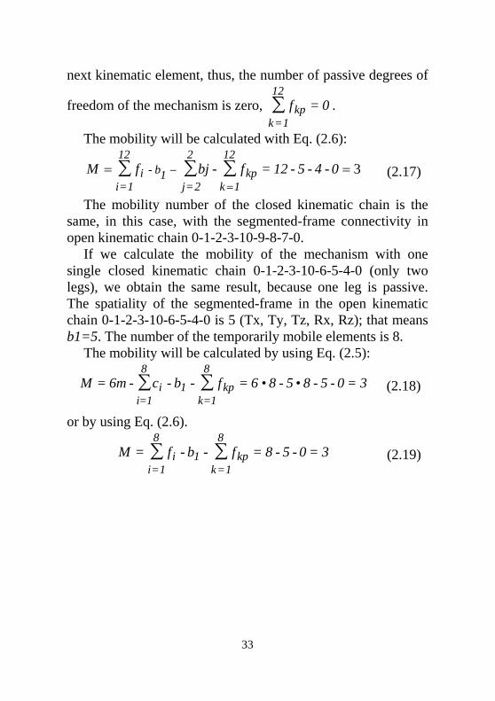
The mobility number of the closed kinematic chain is the same, in this case, with the segmented-frame connectivity in open kinematic chain 0-1-2-3-10-9-8-7-0.

If we calculate the mobility of the mechanism with one single closed kinematic chain 0-1-2-3-10-6-5-4-0 (only two legs), we obtain the same result, because one leg is passive. The spatiality of the segmented-frame in the open kinematic chain 0-1-2-3-10-6-5-4-0 is 5 (Tx, Ty, Tz, Rx, Rz); that means b1=5. The number of the temporarily mobile elements is 8.

The mobility will be calculated by using Eq. (2.5):

3=0-5-8•5-8•6=f-b-c-6m=M8

1=kkp1

8

1=ii ∑∑

(2.18)

or by using Eq. (2.6).

3=0-5-8=f-b-f=M8

1=kkp1

8

1=ii ∑∑

(2.19)

34

2.6 CONCLUSIONS

We consider that the TRIZ method can be utilized even in the case of calculation, where it is required elimination of some contradictions.

We complete the signification of the inventive principle 27 (cheap short-living objects) with a new one: the operation, only mentally, by simple action upon the objects, for a short time.

We underline that the results referring to the formulae for a quick calculation of the global mobility and the interpretation of the notion mobility number were obtained by using the TRIZ method, independently of other methods such as: the one based on the units of single-open-chain, SOC (Yang, Jin et. al., 2002), or the one based on theory of linear transformation (Gogu, 2005).

By using this method, it isn’t necessary to eliminate the passive elements, the passive limbs of the parallel robots, the symmetry from the calculus of mobility of the mechanisms, except the passive degrees of freedom in each joint which do not change the movement of the next element which must be assembled into an open chain.

In our opinion, even if the results are the same, by using TRIZ it is easier to understand a quick calculation of the global mobility of mechanisms.

35

3 TRIZ APPLIED TO FUNCTION GENERATING MECHANISMS

3.1 INTRODUCTION

This chapter presents the study of the function generating mechanisms with variable links length using the TRIZ method.

The mechanisms with variable links length (belt-mechanisms or rolling-bar mechanisms) are used frequently in technical applications for function generation.

The path, function, and motion generation are three classes of coordinated motion studied with priority in the synthesis literature.

Linkages, cam-follower mechanisms, and gears are usually used for this scope.

The bar mechanisms can generate imposed functions only approximately. If there are n - mobile elements, the curves pass through maximum 2n-1 precision points, as Hain K. showed [26].

Many systematic studies about them have been done in the last 3 decades (such as: [26, 27, 28, 29, 30, 31]).

In this chapter some applications are presented: • a function generating mechanism adapted to obtain

functions which differ by constants, • one example which proposes some units of competences

in specified technical domain useful in academic education and • a new model of mechanism with variable links length,

obtained by segmentation of the profiled element.

36

3.2 THE IDENTIFICATION OF SOME TECHNICAL CONTRADICTIONS IN PATH AND FUNCTION GENERATION The function generation problem between two rotating

planar elements is considered. Being important for future analysis, we have identified the

inventive principles recommended by TRIZ, in the field of function generating mechanisms.

A double-crank four-bar-linkage can give a wide variety of functional relationships between its two cranks while both rotate completely.

In this study some technical contradictions are identified, such as:

• To improve the precision of the generated function until absolute precision, but with the ease of operation (in contradiction matrix: manufacturing precision /ease operation, 29/33).

• To improve the precision of the generated function until absolute precision, but with the worsening of the device complexity (in the contradiction matrix: manufacturing precision/ device complexity, 29/36).

• To improve the precision of the generated function until absolute precision, but with the worsening of the length of the moving object (in the contradiction matrix: manufacturing precision/length of the moving object, 29/3). The biggest length of the element is considered initial length.

• To improve the aria of the moving object, but with the worsening of the volume of the moving object, 5/7.

For the 29/33 technical contradiction, the matrix recommends [2]: 1 (segmentation), 32 (color changes), 35 (parameter changes), and 23 (feedback), as inventive principles.

37

For the 29/36 technical contradiction, the matrix recommends [2]: 26 (copying), 2 (taking out) and 18 (mechanical vibration), as inventive principles.



DEVICE COMPLEXITY.DEVICE COMPLEXITY.

…………

…………

...26, 2, 26, 2, 1818

…29


=======Improving

Feature

⇒

⇓26 COPYING2 TAKING OUTSeparate an interfering part or property of an object:separates a property of the changed joint – one degree of freedom, and change the type of the contact, using the superior kinematic joint18 MECHANICAL VIBRATION

For the 29/3 technical contradiction, the matrix recommends

[2]: 10 (preliminary action), 28 (mechanical substitution), 29 (pneumatic and hydraulics) and 37 (thermal expansion), as inventive principles.



LENGTH OF MOVING OBJECT.LENGTH OF MOVING OBJECT.

…………

…………

...10,28, 10,28, 29, 3729, 37

…29


=======Improving

Feature

⇒

⇓10 PRELIMINARY ACTION- perform, before it is needed, the required change of an object (either fully or partially)- pre-arrange objects such that they can come into action from the most convenient place and without losing time for their delivery28 MECHANICAL SUBSTITUTION

29 PNEUMATICS AND HYDRAULICS

37 THERMAL EXPANSION

38

Principle 28 is the mechanics substitution [32]: • to replace a mechanical means with a sensory means; • to use electric, magnetic, and electromagnetic fields to

interact with the object; • to change from static to movable fields, from unstructured

fields to those having structure; • to use fields in conjunction with field-activated (e.g.

ferromagnetic) particles. Referring to this principle - 28, despite the advances in

electronics and electric hardware and software, mechanically coordinated motion cannot be eliminated in many practical applications. Low cost, reduction in weight, consolidation of parts and improved reliability are important advantages of mechanically controlled machines [33].

For the 5/7 technical contradiction, the matrix recommends [2]: 7 (nested doll), 14 (spheroidality - curvature), 17 (another dimension), 4 (asymmetry).


AREA OF MOVING OBJECT.AREA OF MOVING OBJECT.Worsening Feature 7Worsening Feature 7::

VOLUME OF MOVING OBJECTVOLUME OF MOVING OBJECT.

…………

…………

...7, 14, 7, 14, 17, 417, 4

…7


=======Improving

Feature

⇒

⇓7 “NESTED DOLL”- place one object inside another; place each object, in turn, inside the other- make one part pass through a cavity in the other14 SPHEROIDALITY – CURVATURE- instead of using rectilinear parts, surfaces, or forms, use curvilinear ones;- use rollers, balls, spirals17 ANOTHER DIMENSION4 ASYMMETRY- change the shape of an object from symmetrical to asymmetrical- if an object is asymmetrical, increase its degree of asymmetry

•For the belt/band/cable, the inventive princip les:-- “nested doll” – 7, “spheroidality – curvature” – 14, “asymmetry” - 4,“preliminary action” , 10

allow that a long inflexible object to becomes flexible and adaptive on a profiled element.

39

For obtaining rolling-bar mechanisms, three previous contradictions: 29/33, 29/36, 29/3, were unified.

In order to reproduce a wished curve in plane with absolute precision, but with the previous restrictions, the inventive principles: taking out- 2, spheroidality-curvature – 14, and preliminary action – 10, were used.

In order to realize a big area described by a point marked on one mobile element of the mechanism, but with the worsening of the volume described by the moving object, the inventive principles: nested doll – 7, spheroidality – curvature – 14, asymmetry - 4, were utilized.

The inventive principle taking out separates only a property of the changed joint: the number of degrees of freedom (one) and the type of the contact was changed, using at least one superior kinematic joint.

Because we desire to generate an imposed function or path, it is necessary that a point marked on an element follows any point of one curve, so that the lengths of some elements become variable. But it is difficult to coordinate different mechanisms with constant lengths, and the device is complex. It was used the principle spheroidality-curvature: a profiled element defined by a given function was constructed, instead of bar elements and periodic action.

The second element of the superior kinematic pair will be with variable length: a bar or a belt/band/cable.

In the case of a bar, the inventive principles: taking out, preliminary action, and spheroidality – curvature, were applied.

In the case of a belt/band/cable, the inventive principles: nested doll – 7, spheroidality – curvature – 14, asymmetry - 4, and preliminary action allow that a long inflexible object to become flexible and adaptive.

These mechanisms realize elements with variable length during the kinematic cycle of the mechanism.

40

A band mechanism, ‘as some mechanical contrivance that employs a figuratively inextensible flexible element to transmit force and motion from one principal member to another, usually with winding and unwinding without slippage being used on at least one end of the flexible element, or band’, was defined [27].

Several features of the band mechanism recommend it for function generation, such as: controllable backlash, low inertia, and theoretical accuracy.

The Fig. 3.1 shows a mechanism with cable and one rigid element with Archimede’s spiral profile.

Figure 3.1

First contradiction, in this problem, appears between the

cognitive field and the visual field, because it is not so easy to understand the relative motion of one body with respect to the other, if the observer is mobile with respect to both. This contradiction may be eliminated by using the principle the other way round, i.e. to utilize the principle of inverse movement.

For band mechanisms, a simple inversion of the movement with respect to the origin of one rotating element, fixing one of the rotating members, gives a configuration more amenable to analysis.

41

3.3 A FUNCTION GENERATING MECHANISM ADAPTED FOR OBTAINING FUNCTIONS WHICH DIFFER BY CONSTANTS The experimental mechanism shown in Fig. 3.2, from a

scheme of a six-bar function generating mechanism of centroidal type [31] was inspired.

Figure 3.2

The motion can be transmitted only if the force of the spring

tensions the cable. If the flexible element and the circular rigid element of the

mechanism are eliminated, a rigid element mechanism with two driver elements is obtained. The positions of the drivers can be coordinated, but the same movement for the crank-elements of the mechanism with a single driver and variable links length can be obtained.

To generate the functions: C-)ψ(=ψ ϕ (where: ϕ and ψ are the angles of the cranks during the rotation, and C are constants) means to generate equidistant curves. For that it is necessary to eliminate the technical contradiction: improve the area of the moving object, but with the ease of manufacture (in

42

the contradiction matrix: area of the moving object/ ease of manufacturing, 5/32).

For the 5/32 technical contradiction, the matrix recommends [2]: 13 (the other way round), 1 (segmentation), 26 (copying) and 24 (intermediary), as inventive principles.

The inventive principle 1 is segmentation [32]: • To divide an object into independent parts. • To make an object easy to disassemble. • To increase the degree of fragmentation or segmentation. But, in this case, the principle 1- segmentation is: • To divide a period of action into independent parts

(period of time for the preliminary action and period for generating functions) and

• To action only upon a part of the assembly (two linkages: the profiled element and the driver element). The inventive principle the other way round - 13, upon profiled fixed element and driver element was applied: the driver element (AB) rests fixed in a preliminary period of time and the profiled element is rotated.

The constant lengths of the elements, the generating function - )ψ(=ψ ϕ , the starting positions - 0ϕ , 0ψ (Fig. 3.3), and the constant C are known.

The problem is to synthesize the profile element that is suitable for using in the band mechanism and to calculate the α angle of rotation of the profiled element.

The point 0C on the end of the flexible element describes a Γ path (Fig. 3.3) if the mechanism has a spring (Fig. 3.2).

The Γ curve ( )f(=y);f(=x ϕϕ ), using the complex number representation by the known data is obtained.

The Γ curve is the involute of the profiled element (the evolute). The evolute ( )f(=Y);f(=X ϕϕ ) is determinated with Eqs. (3.1).

43

Figure 3.3

''''''

'2'2'

yx-yx)y+(xy

-x=)X(ϕ

''''''

'2'2'

yx-yx)y+(xx

+y=)Y(ϕ (3.1)

The radius of curvature, L , in point (x, y) on Γ curve, with

Eq. (3.2) is calculated.

2)'y''x-''y'(x

3)'2y+'2(x=2y)-(Y+2x)-(X=2L

(3.2)

For 0ϕ and 0ψ input data, the point )y,(x 00 on Γ curve,

the centre of curvature )Y,(X 00 on the evolute of Γ curve, and the radius of curvature 0L are calculated.

44

For obtaining a new function - C-)ψ(=ψ ϕ , and 1Γ path, with the same mechanism, the starting position 0ϕ rests the same, and the second starting position is C-ψ0 .

The parametric equations of 1Γ curve ( Γ and 1Γ are equidistant curves) are determined with complex number representation, but the parametric equations of the evolute are the same: )f(=Y);f(=X ϕϕ .

For C-)ψ(=ψ ϕ function, obtained by rotating the profiled element with α angle, the point )y,(x 11 on 1Γ curve, for input data ( 0ϕ , C-ψ0 ) is determined.

The centre of curvature ( 11 Y,X ) on the evolute, and the radius of curvature 1L , in point ( 11 y,x ), are calculated.

The 1s length of the arch, between )Y,(X 00 and ( 11 Y,X ), with Eq. (3.3) is calculated.

dXY+1=s1

0

X

X

'21 ∫

(3.3) For obtaining C-)ψ(=ψ ϕ function, the angle of rotation

of one circular element, with r radius, with Eq. (3.4) is calculated.

rs+L-L=α 110

(3.4)

45

3.4 EXAMPLE OF UTILISATION OF THE TRIZ METHOD IN ACADEMIC EDUCATION This study and the experimental mechanism (Fig. 3.2) are

useful for the modeling and practical generation of equidistant involutes, of the path contact and the construction of the mating profile useful in Computer Academic Education.

We suggest to university and college students (but not only) that they think critically, practice insight and group learning, for helping them to solve complex problems in technique.

The teachers use the most appropriate methods or strategies of teaching at the undergraduate and graduate seminars for calculation, modelling and practical generation of involute teeth, path of contact and mating profile, following the psychological contents of learning: psychomotor, cognitive and affective [34].

We suggest some competences in a specified technical domain, which are presented below.

The activity is student centred but the interaction is maximal.

• Unit of competence no. 1 To utilize and transpose the mathematical apparatus into a

program for the calculation and modelling of a planar gear with involute teeth.

The conditions to verify the student behaviour It was created a program which calculates the absolute

cartesian coordinates of involute profiles and models the gear (ANNEXE).

The students have the possibility to utilize the computers, and the results of MAPLE program which was realized (Fig. 3.4 and Fig. 3.5 ).

Competence no. 1.1

46

To utilize the notions of evolvent and evolute, various possibilities for the generation of an involute profile, involute function and gear relationships into algorithms.

The wished observable student behaviour We consider a curve defined by parametric equations:

x=x(t), y=y(t); in each point of the curve it may be defined the tangent and the normal. Each of them forms a family of lines depending on parameter t, when the current point describes the curve.

Figure 3.4 Figure 3.5 The family of the tangents generates the curve itself, as

envelope. The normal family to the given curve will generate a new

curve, which is named evolute of the initial curve. In conclusion, the evolute of a planar curve is generated as

an envelope of its normals. The points of evolute curve are centres of curvature in the

points of evolvent curve. The curve named involute is the evolvent of a circle, named

base circle. The involutes are generated by the points of a generating

line which rolls on the base circle.

47

There are other possibilities for generating of the involute profile: as envelope with tangent as cutting edge, rolling on base circle; as envelope with tangent as cutting edge, rolling on rolling circle; as envelope of the mating involute profile, rolling on rolling circle; as path described by starting point of a logarithmic spiral, rolling inside and outside of rolling circle.

The Cartesian coordinates of the current point of the right-sided involute profile with Eqs. (3.5) are calculated:

)180iθarctg-

180iθsin()

180iθ(+1r=x 2

bπππ

)180iθarctg-

180iθcos()

180iθ(+1r=y 2

bπππ

(3.5)

where: br is the radius of the base circle and xinvα=180iθπ .

The Cartesian coordinates of the current point of right-sided involute profile with Eqs. (3.6) are calculated:

]d2s+)

180πα-

180πα2(tg

+180iθ-

180iθsin[arctg)

180iθ(+1r=x

d00

2b

πππ

]d

2s+)

180πα

180πα

2(tg

+180iθ

180iθ

cos[arctg)180iθ

(+1r=y

d00

2b

-

-πππ

(3.6)

where: ds is the tooth thickness on the pitch circle, d is the

pitch diameter, and 0α is the pressure angle of generation.

48

To obtain the coordinates of the intersection point between the left-sided involute profile and the addendum circle Eqs. (3.7) uses:

)x+)r

r-rarctg-

rr-r

sin(r=x Cb

2b

2e

b

2b

2e

e

)y+)r

r-rarctg-

rr-r

cos(r=y Cb

2b

2e

b

2b

2e

e

(3.7)

where: Cx , Cy are the cartesian coordinates of the centre of

the gear and er is the radius of the addendum circle of the gear. To obtain the coordinates of the intersection point between

the right-sided involute profile and the addendum circle Eqs. (3.8) uses:

Cb

2b

2e

b

2b

2ed

00e

x+]r

rrarctg

rrr

d2s

+)αsin[2(tgαr=x

-

--

--

Cb

2b

2e

b

2b

2ed

00e

y+]r

r-rarctg

-r

r-r-

d2s

+)α-cos[2(tgαr=y

(3.8)

The conditions to verify the behaviour of the students If the students can’t realize a complete algorithm, the

teacher will present the algorithm for the calculus of the

49

coordinates of one involute tooth and tooth modeling (Fig. 3.4).

Competence no. 1.2 To transpose the algorithms into MAPLE programs. The wished observable student behaviour To form a combative logical thinking of the students for

technique. To calculate the coordinates of the involute teeth points with

a program. The coordinates of intersection points between the right-

sided involute profile, the left-sided involute profile and the addendum circle may be calculated with the instruction solve in MAPLE program, writing the equations of the addendum circle and the equation of involute profiles, too.

The computational drawing of the gear. The conditions to verify the student behaviour If it is necessary, the teacher presents one program for the

calculus of the coordinates of one involute tooth and tooth modeling.

The students have the possibility to utilize computers. • Unit of competence no. 2 The students compare the obtained programs. They choose the optimal solution from among the solutions

presented by students. The wished observable student behaviour It will be developed the creativity of the students by using

the Brainstorming method, in order to obtain a critical thinking.

The conditions to verify the behavior of the students The students present their own results (modified program)

obtained at the competence no. 1.2. They have the possibility to run and modify the programmes

operating the computers. • Unit of competence no. 3

50

To determine for the given profile the path of contact and the mating tooth profile, point by point.

The wished observable student behaviour Using Reuleaux method it can be determined the path of

contact and the mating tooth profile, point by point, for a given profile.

For each point E1 of the given tooth profile there is a point of the path of contact and a particular point E2 of the mating profile.

The path of contact is the locus of all the points of contact of a pair of tooth profiles with respect to the reference system.

If one profile and the two rolling circles are given, we can construct point by point the path of contact and the mating profile, using the law of gearing.

It will be obtained the practical model of the gear mechanism by students (Fig. 3.6).

• Unit of competence no. 4 To obtain the concordance between theory and practice

verifying the process of gearing, and the law of gearing. The wished observable student behaviour To observe the variation of the point of contact between two

conjugated teeth during the gearing process in the model mechanism.

To verify the curvature of the path of contact described in the model mechanism.

To verify the constancy of the ratio of transmission by measurements of the rotation angles of the gears in different moments of time, in the model mechanism.

The conditions to verify the behaviour of the students. The practical model of the gear mechanism realized by

students, or by teacher, if the students couldn’t realize it (Fig. 3.6).

51

Figure 3.6

• Unit of competence no. 5 To generate the equidistant involutes using the model

mechanism with variable length of flexible element. The wished observable student behaviour To generate an imposed function, or a wished trajectory it

will be introduced in the structure of the mechanism a superior joint, using a cable that is rolling on a profiled element. This mechanism realizes variable length elements during the kinematic cycle of the mechanism.

For the mechanism represented in Fig. 3.2 the motion can be transmited only if a force of a spring tensions the cable. If the flexible element and the circular rigid element of the mechanism are eliminated, it will be obtained a rigid element mechanism with two driver elements.

It can be coordinated the positions of the drivers, but we can obtain the same movement for the elements of the mechanism with a single driver if the mechanism has a circular rigid element and a cable that is rolling on it (Fig. 3.2).

If we want to generate equidistant evolvent curves, we can rotate the circular element around a fixed point. When we

52

rotate the circular rigid element with an imposed angle, the length of the cable and the initial positions of the elements 1 and 2 ( 00 ψ ,ϕ ) are modified. If the initial position of element 1 ( 0ϕ ) is fixed and we rotate the circular element, will be modified only the initial position of element 2 ( 0ψ ). By modifying the initial position of the element 2 we obtain functions which differ by a constant ( const+)ψ(ϕ ).

The conditions to verify the student behaviour Papers, practical model of the mechanism (Fig. 3.2) Supplementary units of competence for graduate student

projects: • Unit of competence To obtain the concordance between theory and

computational modeling by verifying the process of gearing, and the law of gearing.

The wished observable student behaviour To rotate with MAPLE program one gear and its conjugate

gear. To observe the variation of the point of contact between two conjugated teeth during the gearing process in the computational model. To observe the path of contact described in the computational model.

To obtain the angles of rotation of the gears at different moments of time and to calculate the ratio of transmission.

• Unit of competence To calculate the angle of rotation of the circular element of

the mechanism with variable lengths of the flexible element which generate equidistant involutes.

53

3.5 TRIZ APPLIED TO ELIMINATING SOME PHYSICAL CONSTRAINTS IN FUNCTION GENERATING MECHANISMS Another important objective of the study was to utilize the

TRIZ method to eliminate some physical constraints indicated by McPhare (1966): the interference of the profiles, the interference between cable and profile caused by changing the sign of the radius of curvature.

In paper [27] the author investigated the physical constraints on band mechanisms and the application of these constraints to the design equations:

• the band must be unique; • the length of the band must not go to infinity; • the band in last positions must not interfere with the

profile of earlier positions; • in a bi-directional mechanism (requiring two bands and

two profiles), the two profiles must not interfere. We can utilize TRIZ for obtaining complex desired

functions, even though the profiles interfere, and there are inflexion points on profiles.

This case study proposes a new concept for generating complex curves with function generating mechanisms with variable link length, based on the TRIZ methodology.

To obtain complex desired functions, the 35/33 contradiction (adaptability/ease of operation) has been eliminated, by using inventive principles:

- dynamics (15): the reference element has been divided into different plates, with possibility of changing the rotational joint (a particular case: equidecomposable figures);

- segmentation (1) + discarding and recovering (34): profiled element has been divided into different parts which are now fixed on the little plates and some parts are discarded.

54

Periodic action by cable of the profiled elements is possible by changing the position of the rotational joints, by segmentation of the profiled element, and by the forms of the little plates (on which the profiled elements are fixed) which eliminate some relative movements.

One example is presented bellow. The delightful snapshot presented by Steinhaus in 1939 [35]

uses two echidecomposable figures, with four little plates: 1, 2, 3, 4 (Fig. 3.7).

Figure 3.7

On each plate another element is fixed, with different

profile. It can take action with only one motor on the plate no. 4,

actuating through cable the mechanism. Fig. 3.8 depicts the experimental model of this mechanism

actuating through one cable reeled on two reels. For different laws of movement of little plates, the profiled

elements will be designed. Thus, a variable complex mechanism, with variable links

length was obtained.

55

Figure 3.8

In conclusion, the TRIZ method can be used in Computer Academic Education, to etablish some unit of competences and to eliminate some constraints.

56

4 CREATIVITY IN BIONICS

4.1 INTRODUCTION This chapter presents remarks on creativity in the field of

bionics on the author’s opinion. The steps of the strategy in the process of scientific creation

used in bionics, some applications in robotics and academic education are exposed.

Experimental analysis, thought experiments, visual analogy (image representation and relationships, especially mathematical and causal relationships), inventive principles recommended by TRIZ, maintenance of the idea in long-term-memory and intensive attention on it, cognitive historical analysis, were utilized in the process of creativity.

Several structural legged robots were developed, more or less intricate, with movement in plane or in space, inspired from the movement of thousand-legged worms and caterpillars.

The science that uses analogies from biology or botany for solving new engineering problems is named bionics.

Continuity of the authors knowledge of results of previous investigations is useful in many studies.

The history of inventions proves that the maintenance of an idea in long-term memory and intensive attention on it, have had an important role in creativity [36-38]; experimental analysis and analogy are usual tools for it, too.

The visual image plays a central role in the earlier phase, but analogical reasoning can only give probable conclusions.

Thought experiments and calculations are able to verify the presumptions offered by analogies.

Other methods, such as TRIZ, can be used to eliminate the technical contradictions and obtain the final target.

The thousand-legged worms and the caterpillar were selected for this study, the reason being their movement which

57

is so interesting because of their capabilities. For example, the narrow spaces do not raise any problems for them, and complex spatial curves can be easily followed.

The principal features of their locomotion were applied to obtain functional mini-robots, but with few actuators and without intricate structures.

4.2 DESCRIPTION OF THE PROCESS OF CREATIVITY IN BIONICS It is amazing to discover the algorithms of our mind during

creative thinking, the steps in the process of creativity, but it is better to organize the process in advance. In this study, the models were initially created, all the possible analyses were made, and finally creativity techniques were explored.

Different questions referring to the creativity in bionics were asked:

- What is the role of image representation in bionics? - What is the influence of internal or external strain in the

process of creativity? - What is the role of time upon the last activated

remembrance in the process of analogy? - What is the influence of the intensity of the information

stored in the long-term memory in analogical process? - If different steps in the process of scientific creation are

followed, or different creativity techniques studied and presented by others are utilized, will the result of the study in the same domain, for the same problem, be much better, or the same?

The steps forming the strategy used in the study are: A. Morphological analysis of the living creature: the

animal. B. Analysis of locomotion in different directions and on different substrata.

58

C. Brief representation of the initial source – the scheme source. D. Process of retrieval and elaboration of an analogical model – an enhanced source. E. Mapping and transfer between the enhanced source and the probable target. F. Evaluation G. Elimination of the contradictions using the TRIZ method if the probable target does not agree with the wished target. H. The internal or external strain and the comparison by analogy with possible different targets of other inventors. Each of them will be discussed in detail in the following

sections.

59

4.3 STRATEGY

A. Morphological Analysis of a Living Creature: The Animal It was realised a minute morphological analysis, even if in

the future will make a general image representation, because the relationships determined by morphology will be indispensable.

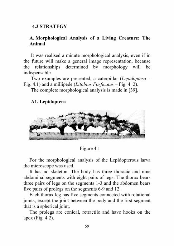
Two examples are presented, a caterpillar (Lepidoptera – Fig. 4.1) and a millipede (Litobius Forficatus – Fig. 4. 2).

The complete morphological analysis is made in [39]. A1. Lepidoptera

Figure 4.1

For the morphological analysis of the Lepidopterous larva the microscope was used.

It has no skeleton. The body has three thoracic and nine abdominal segments with eight pairs of legs. The thorax bears three pairs of legs on the segments 1-3 and the abdomen bears five pairs of prolegs on the segments 6-9 and 12.

Each thorax leg has five segments connected with rotational joints, except the joint between the body and the first segment that is a spherical joint.

The prolegs are conical, retractile and have hooks on the apex (Fig. 4.2).

60

Figure 4.2

A2. Litobius forficatus

The millipede’s body has jointed segments and the exoskeleton of each segment has two parts: the tergum - dorsally placed, and the sternum - ventrally placed, moved by internal muscles.

Figure 4.3

61

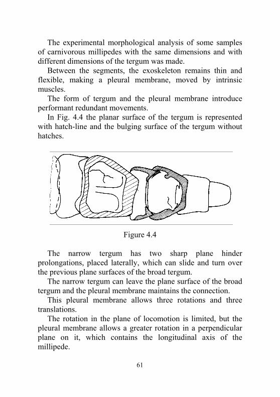
The experimental morphological analysis of some samples of carnivorous millipedes with the same dimensions and with different dimensions of the tergum was made.

Between the segments, the exoskeleton remains thin and flexible, making a pleural membrane, moved by intrinsic muscles.

The form of tergum and the pleural membrane introduce performant redundant movements.

In Fig. 4.4 the planar surface of the tergum is represented with hatch-line and the bulging surface of the tergum without hatches.

Figure 4.4

The narrow tergum has two sharp plane hinder prolongations, placed laterally, which can slide and turn over the previous plane surfaces of the broad tergum.

The narrow tergum can leave the plane surface of the broad tergum and the pleural membrane maintains the connection.

This pleural membrane allows three rotations and three translations.

The rotation in the plane of locomotion is limited, but the pleural membrane allows a greater rotation in a perpendicular plane on it, which contains the longitudinal axis of the millipede.

62

The previous surface of the narrow tergum is a bulging surface and the broad tergum has a hinder plane surface.

Each segment has a pair of appendages placed ventro-laterally and consists of a series of articles, caracteristics common insects (Fig. 4.5 ).

Figure 4.5

The elements of appendages are jointed and can slide ones

into anothers. The coxis forms a spherical joint with the segment of the

body.

63

B. Analysis of Locomotion in Different Directions, on Different Substrata The experiments have great importance in verifying the

presumptions offered by analogies. The experimental research incorporates a high degree of

control over the variables during different processes. This control enables the experimenter to establish causal

relationships between the independent and dependent variables. But these experiments aren’t enough; if you want to change

something old and create something new, you have to give priority to thought experiments, to combine them.

‘The original thought experiment is the construction of a mental model by the scientist who imagines a sequence of evens.

She or he then uses a narrative form to describe the sequence in order to communicate the experiment to others.’ [40].

For this analysis, experiments and thought experiments may be utilised using some TRIZ inventive principles, like the other way round.

It is necessary to obtain the laws of movement. If it is not possible at this step, the process will be cycled

after step (C), when a scheme-source is finished. B1. An application for the principle the other way round, useful in Computer Academic Education It is presented the animation of a four-jointed elements

mechanism which describes a pressed D curve and the principle of opposite movement for designing of stepping mechanisms using the program PASCAL, useful in Computer Academic Education.

64

Our intention is to obtain the competences of the students because it’s necessary to utilize the same units in the process of evaluation.

• Unit of competence no. 1 To transpose the principle of inverse movement into a

programme of animation for a planar mechanism The conditions to verify the behaviour of the students We use a program which realizes the animation of a four-

jointed elements mechanism which describes a pressed D curve, and the animation of the same mechanism using the principle of inverse movement.

The students have the possibility to utilize computers. Competence no. 1.1 To describe the motion of the elements of the mechanism

before and after the principle of inverse movement is applied. The wished observable behaviour of the student The point of planar element which describes in the real

mechanism an approximate rectilinear trajectory, rests fixed by applicating the principle of inverse movement.

The fixed element in the first mechanism becomes mobile during this operation.

It has an opposite motion by comparison with the point with rectilinear motion in the real mechanism and booth have the same modulus of speed.

The conditions to verify the behaviour of the students It is presented only the animation for a four-jointed element

mechanism that describes a pressed D curve. The students have the possibility to utilize computers.Competence no. 1.2 To particularize the program for two opposite positions of

the driver element of the real mechanism. Competence no. 1.3 To indicate the positions of bit end for opposite positions of

the driver element of real mechanism.

65

The wished observable behaviour of student The two bit ends there are on the two different parts of the

curve so: - one of them is on the rectilinear part of trajectory - the other is on the curved part of the trajectory. The conditions to verify the behaviour of the students It is presented the program (ANNEXE) which realizes

superposition of the mechanism for a finite number of positions of the driver element (Fig. 4.6).

The students have the possibility to modify the existing program.

Figure 4.6 Competence no. 1.4 To verify the transposition of the principle of inverse

movement in a program of animation.

66

The wished observable behaviour of student To verify the motions of the elements of the mechanism

before and after the principle of inverse movement is applied. The conditions to verify the behaviour of the students. It is presented the animation of a four-jointed elements

mechanism - which describes a pressed D curve - affected by the principle of inverse movement (Fig. 4.7).

The students have the possibility to utilize the computer program.

Figure 4.7 • Unit of competence no. 2 To adapt the four-jointed elements mechanism to obtain a

legged mechanism. The wished observable behaviour of the student It is considered two four - jointed element mechanisms. We can attach one element to the bit end of each mechanism

so that the free end of the element to be under the level of the fixed element of the real mechanism.

67

We immobilize the driver elements of the mechanisms in opposite positions.

The conditions to verify the behaviour of the students The students can use their own results (modified program)

obtained at the competences no. 1.2 and no. 1.3. They have the possibility to run and modify the program operating computers.

• Unit of competence no. 3 To generalize the process of motion for a legged mechanism

with two four-jointed elements mechanisms. Competence no. 3.1 To observe the period of time in which each leg is fixed on

the ground. The wished observable behaviour of student In the period in which the bit end of the initial mechanism

must be on the rectilinear part of the curve, each leg of the legged mechanism is fixed on the ground.

Competence no. 3.2 To observe the behaviour of the initial base in the same

period of time. The wished observable behaviour of student In this period of time the initial base has an opposite motion

comparison with the point with rectilinear motion in the real mechanism and booth have the same modulus of the speed.

Competence no. 3.3 To observe the behaviour of the antiphasis legs in the same

period of time. The wished observable behaviour of student The antiphasis leg which is on the curved path of the

trajectory advances simultaneously with the initial base because it doesn’t touch the ground and it hasn’t relative movement by comparison with initial base.

Competence no. 3.4 To infer from all the study the complete cycle of motion. The wished observable behaviour of student

68

The leg witch was fixed becomes mobile, the mobile leg becomes fixed and the initial base advances with the same modulus of speed like the speed of the bit end from the real mechanism.

The teacher presents some applications: ’the horse of Cebisev’ and others legged mechanisms with four-jointed elements mechanisms and mechanisms with oscillated slide.

To obtain a critical thinking from the students the teacher proposes to select end points of curve rectilinear portion, because these are necessary for applying the inverse motion principle.

The solutions proposed by students will be discoursed individually or in-group.

Finally, it will be choicen the optimal solution from among the solutions presented by students.

69

B2. Examples in bionics For the study of locomotion of caterpillars and millipedes, a

video camera was used. Some parts from the images were processed on a computer with multimedia system for reduced speed, moderate speed and for the running of the animals on different curves.

B 2.1. The caterpillar The elements of caterpillars that assure the locomotion are

the thoracic jointed legs, the abdominal elastic legs and segments of the body.

The larva walks by looping the body, the wave going from the hind segments to the thoracic segments.

The movement of the body is intermittent. A half of the body is straight and the other is compressed when the larva walks.The centre of curvature is on the intersection of two pairs on the substratum.

For a speed greater than 14 mm/s, the thoracic legs can be raised successively in the air, from the back to the front, three pairs of legs being hanging in the air at a given moment.

Then, the thoracic legs touch the substratum in inverse order with respect to its rising (Fig. 4.8).

For higher speeds, the loop has a larger radius of curvature, and more pairs of legs are in the air.

These observations were easy enough to obtain. B 2.2 Litobius forficatus In the case of the millipede (Litobius forficatus) the

situation was different: the priority was given to experiments on glass, where the creative principle the other way round, presented by the TRIZ method, was applied.

70

Figu

re 4

.8

71

Experiments on glass Initially there was a contradiction between the cognitive

field and the visual field: the movement was seen, but the law of movement could not be understood, going forward and going back, the possible positions of the legs, one towards another, the positions between segments and legs, and the positions of the body segments.

In order to eliminate this contradiction the principle the other way round was used, i.e. to utilize the principle of inverse movement through experiments on glass substratum.

Because the coefficient of sliding friction was not great, the millipede does not advance.

With the help of experimental setup (video camera, computer with multimedia system - Movie Machine, microscope), a base of millipede images during the movement, useful for the analysis of the complex locomotion, was created (Fig. 4.9).

Figure 4.9

I have made many measurements of the angular displacements of the legs with respect to the segments, position of the last segment of the legs, positions of the body segments.

72

Some angular positions of the selected legs: P1, …, P12 (Fig. 4.10 ), with respect to transversal axes of the body segments can be seen in Table 4.1. (unid=unidentified)

Table 4.1

No Time (s)

P1 (0)

P2 (0)

P3 (0)

P4 (0)

P5 (0)

P6 (0)

P7 (0)

P8 (0)

P9 (0)

P10 (0)

P11 (0)

P12 (0)

1 0,4 -45 -40 0 10 0 -22 -35 0 20 27 20 -10 2 0,44 -50 -20 20 0 -25 -27 -20 11 35 12 -25 -30

3 0,48 -55 -10 5 -27 -26 -15 10 30 15 -8 -35 -10

4 0,52 -40 0 0 -27 -27 -12 20 15 8 -10 -32 5

5 0,56 -40 0 -25 -25 -10 10 30 -15 -20 -30 -20 25

6 0,6 -30 -30 -40 -15 10 27 10 -20 -35 -32 10 35

7 0,64 -15 -20 -20 0 27 10 -20 -10 5 25 30 25

8 0,68 -30 -10 10 10 0 -12 -35 10 32 27 15 0

9 0,72 -30 -10 20 0 -20 -27 5 20 35 10 -28 -5

10 0,76 -30 0 0 -15 -27 -5 20 30 15 0 -30 30

11 0,8 -30 0 -10 -20 -22 20 35 10 -30 -20 8 35

12 0,84 -25 -5 -30 -27 -10 27 10 -10 -30 -5 10 36

13 0,88 -10 -25 -25 -15 20 20 0 -30 7 30 30 25

14 0,92 unid -30 -10 -5 27 10 -35 -10 20 35 0 5

15 0,96 unid -15 10 10 -10 -27 -15 20 35 25 -10 -5

The experiments were useful to determinate the laws of

movement. Thus, it was found in Table 4.1 (rows: 9-15; columns: P6-P12) a cyclical law for the direction of rotation of each leg of Litobius Forficatus for a usual type of locomotion: the movement on a straight line. It was observed the laws of the movement of the legs with respect to the body.

73

Figure 4.10

Step 1 t=0 s Step 2 t=0.04 s Step 3 t=0,08 s Step 4 t=0,12 s

74

Figure 4.10

Step 5 t=0,16 s Step 6 t=0.2 s Step 7 t=0,24 s Step 8 t=0,28 s

75

Figure 4.10

Step 9 t=0,32 s Step 10t=0.36 s Step 11t=0,4 s Step 12t=0,44 s

76

Figure 4.10

Step 13t=0,48 s Step 14t=0.52 s Step 15t=0,56 s Step 16t=0,6 s

77

Figure 4.10


78

Figure 4.10

Figure 4.10


79

Step 25t=0,96 s Step 26t=1 s Step 27t=1,04 s Step 28t=1,08 s

80

The antagonistic sets of muscles of the appendages require that each pair of legs to be in straight line, not quite to be ortho on the axis of the body segment.

The angle of rotation for each pair of legs varies from 450 to 1350 and the direction of rotation alternates.

Any two consecutive pairs of legs form an angle of 450 between their axes.

The period of the movement of the legs' wave is at each fifth pair of legs.

At a given moment of time two consecutive pairs of legs are rotating in the same direction, and after two pairs of legs the rotation alternates.

The succession of the leg movement when three legs are intersecting in a centre of curvature is shown in Fig. 4. 11.

.

Figure 4.11

Using the packet of Mathematica programs the functions of

the angular displacements, the angular speeds and the angular accelerations were obtained.

The angular speed varies from 400 0/s to 1000 0/s. The angular acceleration varies from 10000 0/s2 to 50000

0/s2.

81

• Going on the background Positions of the last segment of the legs and angular

displacements of the leg pairs (Fig. 4.12) are presented in the table 4.2; the millipede moves on a paper (t= 0 - 0.44 s). All these dates are reported to a system of coordinates fixed on the background.

The diagrams of angular displacements for seven pairs of successive legs are presented (with dates from table 4.2) in Fig. 4.13.

Figure 4.13

The principle of the inverse movement is: if the final segments of the legs are fixed, the body advances, but the law of action of the muscles is the same.

Using the packet of Mathematica programmes the functions of the angular displacements, the angular speeds and the angular accelerations were obtained. The intervals of time when the legs are fixed on the background were selected.

The functios of some successive legs can be seen below.

82

Figure 4.12

83

Table 4.2

No Time [s]

P2 [mm] ------ [o]

P2' [mm]------[o]

P3 [mm]---- [o]

P3' [mm]----- [o]

P4 [mm]------[o]

P4' [mm]------[o]

P5 [mm]------[o]

P5' [mm]------[o]

P6 [mm]----- [o]

P6' [mm]------[o]

P7 [mm]---- [o]

P7' [mm]---- [o]

1

0,00

-12,9 ------

0

-12.8------

5

-13 ------30

-12.5-------35

-9,5 ------20

-8,5 -------15

-5,6 -------20

-4,8 ------

0

-3,8 ------15

-1 ------20

-3 ------45

1,6 ------20

2

0,04

-13,3 ------

0

-12,8------

5

-13 ------30

-12,5-------40

-9,5 ------20

-8,5 -------20

-5,6 -------20

-4,8 ------

3

-3,8 ------15

-1 ------25

-3 ------45

3,2 ------40

3

0,08

-14 ------ 10

-11,3------20

-13 ------38

-12,5-------30

-8,5 ------

0

-8,5 -------10

-5,6 ------

0

-4,8 ------

0

-4,8 ------30

-1 ------+15

-1 ------

0

4 ------ 50

4

0,12

-14 ------ 25

-11,3------25

-13 ------50

-12,5-------35

-8,5 ------

6

-8,5 -------10

-5,6 ------10

-4,8 ------

0

-4,8 ------40

-1 -------15

-0,4 ------

0

4 ------45

5

0,16

-14 ------ 50

-10,9------30

-9,3 ------

0

-11,3-------25

-6,5 ------

0

-7,7 -------15

-5,6 ------35

-4,8 -------20

-1,6 -------20

2,4 ------45

2,2 -------20

3,4 ------20

6

0,2

-14 ------ 40

-10,9------25

-8,1 -------18

-10,5-------30

-6,5 -------10

-6,9 ------20

-5,6 ------25

-3,6 -------15

-1,2 ------

5

2,8 ------40

2,2 -------15

3,4 ------20

7

0,24

-13,3 ------ 45

-10,9------20

-7,3 -------25

-10,5-------30

-6,5 ------

6

-6,9 -------20

-5,6 ------40

-2,4 ------

0

0,8 -------20

1,8 ------20

2,2 -------20

3,4 ------

0

8

0,28

-11,3 ------ 15

-10,9------

0

-7,3 -------25

-10,5-------45

-6,5 ------25

-6,9 -------20

-5,6 ------35

-2,4 ------

-5

0,8 -------30

1,8 ------15

2,2 ------

0

3.4 ------

5

9

0,32

-10,9 ------

5

-10,9------

0

-8,5 ------10

-10,5-------30

-8,5 ------40

-6,9 -------15

-5,1 ------30

-2,4 ------

0

1,6 -------30

1,8 ------15

2,2 ------15

3,4 ------

5

10

0,36

-9,3 ------ -10

-10,1------

0

-8,5 ------35

-8,5 -------25

-7,3 ------30

-5,7 -------20

-1,8 -------10

-1,6 ------

-5

0,6 -------10

2,4 ------20

1,6 ------25

6,8 ------40

11

0,4

-10,1 ------

0

-9,3 ------

0

-9,3 ------35

-8,3 -------20

-6,1 ------20

-5,1 -------20

-1,2 -------15

-0,8 ------

0

0,6 -------10

3,2 ------30

1,6 ------30

7,6 ------40

12

0,44

-11,7 ------ 30

-7,3 ------15

-10,5------45

-7,7 -------20

-4,9 ------10

-4,4 -------15

-1,2 ------

0

-1,2 -------10

-0,4 ------25

3,2 ------15

1,6 ------40

7,6 ------40

84

For the leg P2 (the interval of time: 0,08 s - 0,2 s): ϕ (t)=-394 + 13611.7 t - 170646 t2 + 947396 t3 - 1.90104 106 t4

'ϕ ( (t) =13611.7 - 341292 t + 2.84219 106 t2 - 7.60417 106 t3 ''ϕ (t) =-341292 + 5.68438 106 t - 2.28125 107 t2

For the leg P3 (the interval of time: 0,035 s - 0,13 s): ϕ (t)=24.9201 + 542.673t - 19737.3 t2 - 1.15411106 t4

'ϕ ( t) =542.673 - 39474.5 t + 839396 t2 - 4.61644 106 t3 ''ϕ ( t) =-39474.5 + 1.67879 106 t - 1.38493 107 t2

For the leg P4 (the interval of time: 0,16 s - 0,28 s): ϕ (t) =652.108 - 8276.34 t + 30776 t2 - 23052.9 t3 - 29440.1 t4 -18030.5 t5 - 8442.69 t6 - 3418.15 t7

'ϕ (t) =-8276.34 + 61552 t - 69158.7 t2 - 117761 t3 - 90152.6 t4

- 50656.1 t5 -23927 t6 ''ϕ (t) = 61552-138317 t - 353282 t2 - 360611 t3 - 253281 t4 -

143562 t5 For the leg P5 (the interval of time: 0,039 s - 0,29 s): ϕ (t) =665.473-58187.6 t + 1.95698 106 t2 - 3.40783 107 t3 + 3.40674 108 t4 - 2.01999 109 t5 +7.0013 109 t6- 1.30817 1010 t7 +1.01658 1010 t8

'ϕ (t) = -58187.6 +3.91395 106 t - 1.02235 108 t2 + 1.36269 109 t3 - 1.00999 1010 t4 + 4.20078 1010 t5 - 9.15718 1010 t6 + 8.13263 1010 t7

''ϕ (t) = 3.91395 106 - 2.0447 108 t + 4.08808 109 t2 - 4.03997 1010 t3 + 2.10039 1011 t4 - 5.49431 1011 t5 + 5.69284 1011 t6

The angular speed varies from 400 0/s to 1000 0/s. The angular acceleration varies from 10000 0/s2 to 50000

0/s2. Positions of the centres of mass of body segments (Fig.

4.12) are presented in the table 4.3.

85

Tabl

e 4.

3

t

t [s]

G1

G2

G3

G4

G5

G6

G7

x[

mm

] y[

mm

] x[

mm

] y[

mm

] x[

mm

] y[

mm

] x[

mm

] y[

mm

] x[

mm

] y[

mm

] x[

mm

] y[

mm

] x[

mm

] y[

mm

] 0

-16,

7 -1

,07

-13,

9 -1

,07

-10,

9 -1

,28

-8,1

4 -0

,64

-5,3

6 -0

,43

-2,5

7 0,

21

0 0,

86

0,04

-1

6,7

-0,8

6 -1

3,9

-0,8

6 -1

0,9

-1,0

7 -8

,14

-0,6

4 -5

,36

-0,2

1 -2

,57

0,43

0

0,86

0,

08

-16,

7 -1

,5

-13,

9 -1

,5

-10,

9 -1

,07

-8,5

7 -0

,64

-5,3

6 0

-2,5

7 0,

43

0 0,

86

0,12

-1

6,2

-1,5

-1

3,5

-0,8

6 -1

0,9

-0,4

3 -8

,57

-0,4

3 -5

,36

0 -2

,57

0 0

0,64

0,

16

-15

-0,6

4 -1

2,2

-0,4

3 -9

,86

-0,2

1 -6

,86

0 -3

,64

0 -1

,28

0,43

1,

71

0,43

0,

2 -1

3,7

-0,6

4 -1

1,3

-0,4

3 -8

,99

-0,4

3 -6

,21

-0,4

3 -3

-0

,21

-0,6

4 0,

43

2,36

0,

64

0,24

-1

3,2

-0,6

4 -1

0,9

0 -8

,14

0 -5

,78

0 -2

,57

0 0

0,64

2,

78

0,64

0,

28

-13,

2 0

-10,

9 0

-8,1

4 -0

,21

-5,1

4 -0

,21

-2,1

4 0

0 0,

64

2,78

0,

64

0,32

-1

3,2

0 -1

0,9

0 -8

,14

0 -5

,14

0 -2

,14

0,21

0

0,64

2,

78

1,07

0,

36

-12,

6 -0

,21

-10,

5 0

-6,8

6 0

-4,7

1 0

-2,1

4 0

0,43

0,

64

3,43

0,

86

0,4

-12,

6 -0

,21

-9,8

6 -0

,21

-6,8

6 -0

,21

-4,2

8 -0

,43

-15

0,21

0,

64

0,43

3,

86

1,28

0,

44

-12

-0,2

1 -9

,86

-0,2

1 -6

,86

-0,2

1 -4

,28

0 -1

5 0

1,28

0,

43

4,28

1,

07

86

Using Mathematica packet of programs, the functions x(t), y(t), x'(t), y'(t), x''(t), y''(t), of the centre of mass of body segments were obtained.

The maximum speed of the centre of mass of body segments is 35 mm/s in the direction of x axis and 10 mm/s in the direction of y axis.

The maximum acceleration of the centre of mass of body segments is 500 mm/s2.

These two experiments (on glass and on background) revealed the independent movement of the body segments and the movement of the appendages with respect to the body.

The relative position of the legs and the kind of action of the joints are the same as those presented in the movement on glass, but the legs touch the background.

The succession of the legs that are in contact with the background are presented bellow (L=left, R=right).

For the going forward, following a curve in plane with a straight axis, the support is provided by the following legs: L1, R2, R3, L4, L5, altering with L1, L2, R3, R4, L5, altering with R1, L2, L3, R4, R5, altering with R1, R2, L3, L4, R5.

For the going back, following a curve in plane with a straight axis, the support is provided by the following legs: R1, L2, L3, R4, R5, altering with R1, R2, L3, L4, R5, altering with L1, R2, R3, L4, L5, altering with L1, L2, R3, R4, L5.

For the going forward, following a curve in plane with a curve axis, the support is provided by the following legs: L1, L2, R3, R4, L5, altering with L1, L2, L3, R4, R5, altering with L1, L2, L3, L4, R5, altering with L1, L2, L3, L4, L5, altering with R1, L2, L3, L4, L5, altering with R1, R2, L3, L4, L5, altering with L1, R2, R3, L4, L5.

87

It was concluded the law for straight movement: the legs that are on the curve of the body, at a given moment, from an inflexion point to the next, exclusively, which are intersecting in the centre of curvature, touch the substratum, and the corresponding legs in the same pairs are lifted. This feature is also valid for curves with a greater radius of curvature. The number of the legs is proportional to the dimension of the radius.

For the going back, the legs that are on the curve of the body, at a given moment, from an inflexion point to the next, exclusively, which are intersecting in the ce+ntre of curvature, are lifted, and the corresponding legs in the same pairs touch the substratum. The action modality of the muscles is the same for the forward walking, only the points of contact with the substratum are others.

For traveling on a curve all the elements that are in the centre of curvature touch the substratum with the help of sliding or rotational joints and all kinematic chains in this curve are inactive until the mechanism changes the direction. The passive chains have a rotational movement around the centre of curvature, until the first element reaches the limited position (at 450 in the direction of travel). After this, each element follows the previous law of movement.

88

C. Brief Representation of the Initial Source – The Scheme Source

This step is considered by the author to be very important:

the realization of a scheme of the source according to the principal purposes of analysis; by discarding irrelevant relationships in the initial source and storing critical ones, a new scheme-source can be obtained. The author considers the visual analogy the basis of scientific creation in bionics.

This first enhanced source - the scheme-source with selected relationships, especially mathematical and causal relationships - will be the new source-model. Both image representation and analogical reasoning must be used for creating new models. Some examples are presented below.

The morphological analysis, the analysis of the movement in different conditions, on different substrata, on different curves, in plane or in space, help at realization of simplified schemes.

Some schemes focus on the specific relationships of the phenomena.

Fig. 4.14 depicts a simplified scheme, with visual similarities with respect to the animal during locomotion.

The same figure, a triangle, was observed between the elements of the ‘body’.

This idea was stored in the memory, because it might be useful later.

This scheme was used for a spatial mechanism [41]. Some geometrical restrictions and relationships which

establish the laws for different types of movement, useful to create new planar or spatial mechanisms were added to this scheme.

The positions of the legs and their law of movement in plane were kept, but the form of the body was simplified, using the same allure, like a wave.

89

Figure 4.14

The elements: 1, 2, 3, 4, 5 (Fig. 4.14) were reduced to ‘beam’ type elements: 1, 2, 3, 4 (Fig. 4.15). The elements 1, 2, 3, 4, are midlines in the resulting triangles (Fig. 4.15).

Figure 4.15 In the case of the movement of Lepidoptera, we store the

scheme of some jointed elements in a serial linkage, but with a grate facility for compactness, change of direction and for torsion.

90

D. Process of Retrieval and Elaboration of an Analogical Model – an Enhanced Source The process of retrieval and elaboration of an analogical

model to develop an enhanced source used the scheme-source which is common in both, the crude and the target domains.

Two examples can be seen below. For the caterpillar (Lepidoptera), some complex structural

models (Fig. 4.16 and Fig. 4.17) of walking robots with rigid elements were realized.

But, they were too complicated, with too many actuators, leading to the conclusion that the targets are not acceptable.

This strain influences on our minds.

… Figure 4.16

Fig. 4.17

The base of images of the Litobius forficatus was useful to

realize the structural models by analogy. A complex structural model of one walking robot was made

and analyzed (Fig. 4.18).

91

LS

D12

LS

D11

LS

D10

LS

D9

LS

D8

LS

D5

LS

D4

LS

D13

LS

D7

LS

D3

LS

D6

LS

D2

LS

D1

157

156

25

2 25

1

25

0 24

9

24

8

24

7

24

6

24

5

24

4

24

3

24

2

24

1

24

0

23

92

38

23

7

23

6

23

52

34

23

3

23

2

23

1

23

0

22

9

22

8

22

7

22

6

22

52

24

22

3

22

22

21

22

0

219

218

217

216

215

214

213

212

211

2102

092

082

07

206

205

204

203

202

201

200

199

198

197

196

195

194

193

192

191

190

189

188

187

186

182

185

184

183

181

180

179

178

177

176

175

174

173

172

171

170

169

168

167

166

165

164

163

162

161

160

159

158

155

154

153

152

151

150

149

148

147

146

145

144

14314

2

141

140

139

138

137

136

135

134

133

132

131

130

129

128

127

12612

5

12412

3122

121

115

120

119

118

117

116

114

113

112

111

110

109

108

107

106

93

105

104

103

102

101

100

99

98

97

96

95

94

92

91

90

89

88

87

86

85

84

83

828

1

80

79

78

77

76

7574

737

27170

69

68

67

66

65

64

63

62

61

60

59

58

57

56

555

453

5251

50

49

48

47

46

45

44

43

42

41

40

39

383736

35

34

33

32

31

30

29

28

27

26

4

25

24

23

22 2

12

0

19

18

1716

15

14

13

1211

10

9

8

76

5

3

21

Figure 4.18

92

E. Mapping and Transfer from the Enhanced Source to the Probable Target This step continues the process and is completed by

evaluation. Some examples can be seen below. The specific features of the millipede locomotion were kept,

for different types of locomotion creating different stepping mechanisms [41].

The simplified body in different positions in the plane was drawn (Fig. 4.19).

The sustained triangular form (or like a cone) in different positions in plane was observed. Attempts were made to rotate the triangles (or cones) from one position to the next to obtain the desired positions in plane.

Figure 4.19

93

And thus, a spatial structural model inspired from these schemes was created.

Fig. 4.20 represents the new structural model of robot MMS5.

The structural model has 17 rigid elements, 12 joints of rotation (C, D, E, F, G, H, I, J, M, N, O, P) and 4 cylindrical joints (A, B, K, L).

The elements 1, 2, 3, 4, 5 are cylinders and 10, 11, 12, 13 could be cones or triangles.

The elements 14, 15, 16, 17 can be rotated in the joints N, M, P, O, at different moments.

Figure 4.20

While it is in plane, the form of the mechanism is the same

as the millipede’s body during some periods of the movement. The cones could have some channels, and some spherical

elements can be between the cones and the cylinders.

94

F. Evaluation All process is completed by evaluation.

F. 1 Model MMS5

The picture of the model MMS5 can be seen in Fig. 4.21.

Figure

Figure 4.21

The mechanism could have different laws of movement in space, according to the kind of action of the leading joints.

But, while it is in-plane, the form of the mechanism is the same as the millipede’s body during some periods of movement.

95

Having applied thought experiments you can try to realize some experiments to certify your new theory (Fig. 4.22).

Fig. 4.23 and Fig. 4.24 depict the direction of rotation of the elements of the robot, during a complete cycle, for motion from right to left and from left to right, respectively.

Figure 4.23

Figure 4.24

96

Figure 4.22

97

I realized the program (ANNEXE) using partitioned matrix algebra ([42]) to calculate:

- the matrices of base change, - the generalized coordinates, - the angular speeds, - the matrix with the partial angular speeds, - the absolute angular speeds and the absolute accelerations

of the kinematical elements, - the absolute speeds and accelerations of some points of

kinematical elements. Each kinematical element was associated with its

CARTESIAN system of coordinates, with base of vectors:

Tiiii= 321 iiii

→→→→.

The E absolute reference was associated with the base of

vectors T0→0→0→0→

= 321 iiii and the element j with the P system.

In general case, the E system will be rotated three times, until its axes are identical with the axes of P system (Fig. 4.25).

Because the rotation of the E system around its three axes with unchanged angles, but following other succession, generates a system with other orientation, it is necessary to be attentive at the forms and known movements of the elements of the mobile system.

For the transformation of the E system into the P system, we use Eq. (4.1).

i0→

]PSE=[i→

(4.1)where ]S[ PE is calculated with Eq. (4.2).

]S][S][S[]S[ 12132 EEEEEEPE = (4.2)

98

.

Figure 4.25

Considering the element j with respect to the element k and the three angles which give the orientation of the system Rj with respect to the system Rk (which are met in the matrix of base change ]S[ kj ) we consider:

Tk3

k2

k1

kR

k φφφ=q=φ . For a system with n rigid elements joined by rotational

links, the generalized coordinates are components of the vectors: n1,=k,qk

R ; that means 3n geometrical parameters, which are noted: 3n21 q,...,q,q .

The vector of the generalized coordinates is:

99

T3n21

TnR

2R

1RR ...qqq=...qqq=q=q

In the case of this model, MMS5, we can’t rotate all systems in the same previous succession and keep so one single form for the matrix of base change ]S[ kj , because the knowledge of angles of rotation is very difficult in that succession.

Each system will be rotated first with constant angles around certain axes and finally with variable angle until the system will be transformed into the system of the following element.

The first system in this process will be the absolute reference.

The succession of rotations for the transformation of the systems there is (Fig. 4.26):

- the transformation from the system 0 into the system 1, by rotation around z0 axis with the angle 3

oq (this operation isn’t

presented in Fig. 4.26); tφ=q 133

o & ; 0=q=q 2o

1o .

- the transformation from the system 1 into the system 2, by rotation around y1 axis with the angle 2q ;

tφ+-180=q 222 & ; 0=q=q 31 .

- the transformation from the system 2 into the system 3, by rotation around z2 axis with the angle o45- ; one rotation

around y2 axis with the angle 5q ; tφ=q 325 & ; o

6 -45=q . - the transformation from the system 3 into the system 4, by

rotation around x3 axis with the angle o180 ; one rotation

around z3 axis with the angle o225 ; one rotation around y3 axis with angle 8q ; tφ=q 4

28 & ; o7 180=q ; o

9 225=q .

100

- the transformation from the system 4 into the system 5, by rotation around z4 axis with the angle o45- ; one rotation

around y4 with the angle 11q ; tφ=q 5211 & ; o

10 0=q ; o

12 45=q - .

Figure 4.26

The matrices of base change for robot MMS5 are given by

relations (4.3).

101

⎥⎥⎥

⎦

⎤

⎢⎢⎢

⎣

⎡

1000cs-0sc

=]S[ 33

3310 ;

⎥⎥⎥

⎦

⎤

⎢⎢⎢

⎣

⎡

22

2221

c0s010s0c

=]S[-

;

⎥⎥⎥

⎦

⎤

⎢⎢⎢

⎣

⎡

23232

33

2323232

csscs0csssccc

=]S[ --

;

⎥⎥⎥

⎦

⎤

⎢⎢⎢

⎣

⎡

121321213232

13133

12132121323243

cc+ssssccsscsscccs

cssscss+csccc=]S[

--

-

⎥⎥⎥

⎦

⎤

⎢⎢⎢

⎣

⎡

23232

33

2323254

csscs0csssccc

=]S[ --

(4.3) We associate for each element i the 1+iwr vector, where:

1+ii1+i OO=wrr .

Oi represents the origin of the Ri system and Oi+1 the origin of the Ri+1 system, associated with the element i+1.

M1, M2, M3, ......, Mj are points of the kinematic elements for which it will be determined the speeds with respect to the global R0 system.

The vector of position of Mj point, with respect to R0 system, is given by Eq. (4.4).

∑j

1=i

0j0Tj

01-i0Ti

RM i]S[r+i]S[w=r 0

j

rrr

(4.4)

To determine the angular speed it will be used equation (4.5).

102

Tjojojo ]S][S=[]Ω[ & (4.5)

where:

[ ]⎥⎥⎥⎥

⎦

⎤

⎢⎢⎢⎢

⎣

⎡

0ωω

ω0ω

ωω0

=Ωj

10j

20

j1

0j3

0

j2

0j3

0

jo

-

-

-

(4.6)

We note:

)ω,ω,ω( j3

0j2

0j1

0 like ω=)ω,ω,(ωω jjjj

j0

321

→ .

We calculate the angular speed of the element j with respect to the global system, with equation (4.7).

i]S[ω=ω 0j0j

j→0 r

(4.7)

Deriving the vector of position of one point Mj with respect to time we obtain the speed of the point with respect to Ro and deriving it two times we obtain its acceleration.

The program was run with the angular speed of the leader element = 83 rpm, similar to those of the Litobius forficatus for the period of time 0 - 0,349 s.

The dimensions of the elements were: length of the cylinder =10 mm; radius of cylinder=4 mm; length of the element which corresponds to the leg of the millipede =12,071mm; angle of the cone =450.

The results denote that the chosen geometry of the mechanism partially respects the kinematic of the millipede. The mechanism imitates the movement of millipedes in different successive positions in plane.

The number of actuators is 4 or 5 at a given moment.

103

G. Elimination of Contradictions Using the TRIZ method if the Probable Target Does Not Agree with the Wished Target If the probable target does not agree with the wished target,

the contradictions will be eliminated using the TRIZ method, becoming the new enhanced source. After this, the steps (E) and (F) are repeated.

Consciously or intuitively, everyone eliminates contradictions when they create something new in the domain of science or technique.

G1. The millipede In this work there were many technical contradictions, such

as: - To keep the same main law of the locomotion of the

animal’s body in plane, but with the simplest possible structure (in the contradiction matrix: adaptability/device complexity, 35/36);

- To keep great mobility, but with few actuators (in the contradiction matrix: adaptability/ease of operation, 35/33);

- To move in narrow spaces, with the same main law of movement of the animal, but without the great volume of the robot (in the contradiction matrix: adaptability/volume of an object that is moving, 35/7).

For the 35/36 technical contradictions, the matrix recommends: 15 (dynamics), 29 (hydraulic or pneumatic), 37 (thermal expansion), 28 (mechanics substitution).

For the 35/33 technical contradictions the matrix recommends: 15 (dynamics), 34 (discarding and recovering), 1 (segmentation) and 16 (partial or excessive action) as the inventive principles.

These two contradictions were unified.

104

In order to reproduce principal types of locomotion of the millipedes in plane, but with a simple device with minimum of motors, the inventive principles: discarding and recovering - 34, merging - 5, periodic action - 19, mechanics substitution - 28 and dynamics – 15, were used.

It was used a simplified scheme, obtained by: (a) discarding irrelevant degree of freedoms of some kinematic elements (inventive principle discarding and recovering - 34); and (b) assembling similar parts, different kinematic elements of the legs - to perform parallel operations: the same movement of the new legs (inventive principle merging -5).

Priority was given to the coordination of the movement with a minimum of number actuators.

Many ideas which were including the previous scheme were considered resulting in:

- the use of electromagnetic fields, fixing some points of legs (inventive principle 28) and

- a design process to find an optimal number of actuators by using one single rotational motor (inventive principle 15).

The periodic action (inventive principle 19) of the actuators was presented in [39], for different types of locomotion.

Fig. 4.27 depicts the new simpler structural model. For this model it is interesting to remark that one single

motor with alternating rotation (in joint B), and two actuating sliding or rotational joints on each of the ‘body’ elements (in joints: A and C1; M and C2; G1 and C3; G2 and N; G3 and O ...) are sufficient for the locomotion of this multi-legged mechanism, even if the set of four body-elements (Fig. 4.27) is repeated.

105

Figure 4.27

The robot presents certain geometrical restrictions established by analogy with the initial source, according to the morphological analysis: the elements 2, 4, 6, 8 ... are midlines in the passive chains.

There are variable kinematic chains during the locomotion which alternate from active to passive.

It was possible to establish the law for the command of the actuators on different curves in plane.

We choose a structural model with 5 pairs of legs (Fig. 4.28).

The structural model (Fig. 4.28) has 39 rigid kinematic elements, 45 rotation joints plus joints that are formed at the contact with the background (Fig. 4.28).

The segments of the body are substituted with the elements 1, 3, 5, 7, 9 and the ‘legs’ P1,..., P10 are situated at the end of these elements.

106

Figure 4.28

For this structural model some characteristics of one type of displacement of millipedes are used.

The projections of the legs on the horizontal plan are constant. It is respected too, the law of setting of the legs on the background.

The structural model presents variable chains during locomotion.

For the kinematic calculus it was useful vectorial method and it was made a program in PASCAL language (ANNEXE).

It was determinated the optimal dimensions of the mechanism that realise displacement with the same kinematic parameters like real millipedes.

The principal goal was to obtain the same angular speeds for all equivalent elements of animal body segments, the same angular speeds for all equivalent elements of animal pair legs, with minimum of actuators.

107

For that, the dimensions of mechanism elements must respect the following conditions:

- for the value l1 adopted, the length l2 is determined with Eq. (4.8):

)cos45-(121

l=l 012

(4.8)

- the point D coordinates are determined with the condition: ∧

ADC = 450 (for the limited position). The angular speed of the first pair of legs of the millipede

was determined experimental with the help of the films (measurements and processing of the dates):

'ϕ =5000 /s; n=83 rpm.

For the kinematic calculus of the mechanism it was utilised n=83 rpm, l=13,5 mm (like the real dimension of the sample).

With the obtained results it was realized the diagrams of angular positions, speeds and accelerations, with 1ϕ from 450 to 900.

Compared with experimental measurements, the theoretical angular speed and acceleration are approximately equal.

s/erimentalexp0450≈ω ; s/ltheoretica

0050≈ω ;

2010000≈ s/erimentalexpξ ; 207000≈ s/ltheoreticaξ

108

It was created a program in TURBO PASCAL planning to visualize the moving of the mechanism in curves, like in the Fig. 4.29.

Figure 4.29

The animation of the mechanism denotes a similitude with the real trajectory of the millipede during the movement.

h) g)

e) f)

d) c)

b) )

c) d)

e) f)

g) h)

a) b)

109

The experimental model can be seen in Fig. 4.30. The dimensions of this model are: length = 0,4 m, width=

0,13 m, height= 0,08 m. The type of the model is planar multi - legged robot. It weighs 1 kg and has a maximum velocity of 0,1 m/s.

Figure 4.30

110

To eliminate the contradiction: adaptability/volume of an object that is moving, 35/7, one of the inventive principle recommended in contradiction matrix, dynamics- 15 was used, in addition to merging- 5, thermal contraction- 37 and spheroidality-curvature- 14.

The robot shown in Fig. 4.30 can be adapted, becoming flexible, using shape memory actuators and flexure hinges.

By analogy shape memory actuators instead of rotational motors there are used, going from the idea that the muscles have three specific properties: elasticity, excitability and contractibility.

Thus, the inventive principle thermal contraction is applied, utilizing SMAs (shape memory alloys), which are metals that ‘remember’ their original forms. SMAs can change shape, stiffness, and other mechanical characteristics in response to temperature and stress.

Another inventive principle that was applied for the same contradiction was spheroidality-curvature.

For this reason flexure hinges were used instead of rotational joints.

The material of the mini-robot will allow it to become flexible (the principle: dynamics).

But, the law of movement on any curve in plane is the same, and thus the control for leading the ‘legs’ and for the main actuator is unchanged.

Results from an analysis with FEM (finite element method) using the COSMOS program for different situations [43], showed that the areas of flexure hinges were most stressed (Fig. 4.31).

111

Figure 4.31

112

H. The Internal or External Strain and the Comparison by Analogy with Possible Different Targets of Other Inventors The history of technique proves that the maintenance of one

idea in long-term memory, the intensive attention on it and the visual analogies has had an important role for creativity.

When Isaac Newton was asked about his method used in research he answered: I was thinking about a problem, I was keeping the subject of my research before my eyes, looking forward to the first light of my mind, until it has changed into a clear idea.

It is said that the great inventor Michael Faraday was keeping in the pocket of his waistcoat a little magnet to remind him the most important preoccupation during his entire career.

If he was occasionally touching the magnet during the lecturers, all the students were leaving the class in silence because they knew that the great teacher was thinking to the electromagnetism.

If an acceptable target is not found, and an internal or external strain influences the inventor, the selected scheme-source will be compared by analogy with possible different targets of other inventors, which are stored in the long-term memory or with other new possible targets that can be seen in the future.

We consider that this last complex process begins from the present to the past and it is furthered by cognitive historical analysis.

In this comparison, visual similarities with the primordial wished relationships are mapped.

If we obtain an acceptable model from the long-term memory, the process will be continued with transfer and evaluation, and can be repeated.

113

Some examples can be seen below. For Lepidoptera, some complex structural models of walking robots with rigid elements were realized (Fig. 4.16 and Fig. 4.17). But, they were too complicated and had too many actuators leading to the conclusion that the targets were not acceptable, resulting in strain that influences the mind.

The scheme-source of Lepidoptera deduced from the complex model has permanently rested in the mind.

It is compared by analogy with different targets of other authors, stored in the long-term memory.

This process begins from the present to the past. It is fixed on the last most impressive remembered image

with visual similarities and the primordial wished relationships. Our attention was fixed on the delightful snapshot presented

by H. Steinhaus in 1939 without details (Fig. 4.32): two echidecomposable figures (the square and the equilateral triangle) and four little plates which compose the square or the triangle.

The inventor wrote: If we turn the lever up or down, with these four little plates

we are able to compose a square or an equilateral triangle. Boltyansky defines two figures from the plane being

echidecomposable if one of them can be decomposed in a finite number of parts that can be reorganized to form the second figure (Fig. 4.33).

Schoenberg presented in 1989 the construction of these four plates [35] (Figure 4.34).

114

Figure 4. 32

c

d

c

b

aa

Figure 4.33

c

115

Figure 4.34

A program in TURBO PASCAL was created, for kinematic

calculus and simulation of the motion of a planar mechanism, that realizes a circular movement of the figures, alternating the square with the triangle (Fig. 4.35, Fig. 4.36).

Figure 4.35

116

Figure 4.36

Mapping and transfer from the enhanced source to the

probable target continue the process: we agree with the new mechanism, but our preoccupation is to realize a walking mechanism; for that, the plate a (Fig. 4.31) will be mobile.

We combine the experiments with thought experiments. We observed that this mechanism presented by Steinhaus can be used for the creation of a planar mechanism.

It reproduces a circular movement of the figures, alternating the square with the triangle (Fig. 4.37), or can reproduce the movement to right or to left (Fig. 4.38).

Figure 4.37

117

Figure 4.38

For a circular movement one or another marginal plate is

fixed alternatively. It can use the three leading joints (each of them turned with 1800) or it can take action with only one motor on the plate a (respectively d), actuating through cable the plates b, c, d (respectively a, b, c). The cable pass over the circular plates fixed on each plate.

Fig. 4.39 depicts the experimental model of this mechanism actuating through one cable reeled on the two reels (Fig. 4.40).

If we attach ‘legs’ to each little plate, it must be taken into account that when the little plate is moving, the ‘legs’ must be raised from the substratum and when the little plate is fixed, the legs must be in contact with the substratum.

Figure 4.39 Figure 4.40

118

4.4 CONCLUSIONS

Bionics may be used successfully to create new walking

robots. The conclusions of the author after this study are

synthesized in the answers to some questions: - What is the role of the image representation in the domain of bionics? Visual analogy is the basis of scientific creation in bionics. This phase is so important because the scheme-source with

selected relationships, especially mathematical and causal relationships, will be the new source-model.

By discarding irrelevant relationships of the initial source and storing critical ones, a new scheme-source will be obtained.

- Is it right to realize a minute morphological analysis and a minute analysis of locomotion, or is it better only to look at the general aspects of them?

It is right to obtain the relationships determined by morphology and main features of the locomotion; and finally, it is useful for the exercise (algorithms) of the mind.

- What is the role of internal or external strain in creation in bionics?

It drives to eliminate the technical contradictions (intuitively or not) or to find in the long-term memory the results of other inventors, or to continue the process of analogy in the future.

- What is the influence of time upon the last activated remembrance in the process of the analogy?

This process begins from the present to the past. - Why were some realizations from the history of science

selected and utilized and not others?

119

The influence of the intensity of the information stored in the long-term memory is very important in analogical process.

The last most impressive (positive or negative) remembered image, with visual similarities and the primordial wished relationships is fixed.

If internal or external strain forces to a continuity of the process, the next most impressive remembrance from the present to the past is fixed.

- If different steps of the process of scientific creation are followed or different creativity techniques studied and presented by others, will the result of the work in the same domain, for the same problem, be better, or the same? Probably it will be better.

ANNEXE

120

5.1 PROGRAM FOR A KINEMATIC CALCULUS OF THE MECHANISM MMS4 uses crt,dos,printer; type vec=array[0..360] of real; var xd,yd,xf,yf,xfp,yfp,xfpp,yfpp,xg,yg,l1,l2:real; vf3,vfxc,vfyc,vf2dd,vf2,vf3d,vf2d,vf3dd,vcxd,vcyd,vcxdd, vcydd,vf3r,vf2r,vfxcr,vfycr,vf3dr,vf2dr,vf3ddr,vf2ddr,vcxdr, vcydr,vcxddr,vcyddr:vec; aa:char; fi1,lab,lbc,lcd,n1,xb,yb,fi2,fi3,fi4,fi5,a,b,c,xc,xcr,yc, ycr,xm,ym,pix,pix1,xcpr,ycpr,xcppr,ycppr:real; var fi2p,fi3p,fi2pp,fi3pp,fi4p,fi5p,fi4pp,fi5pp,xcp,ycp,xcpp, ycpp:real; var fi1p,xbp,ybp,xbpp,ybpp,t1,t2,xdp,ydp,xdpp,ydpp:real; var i:integer; procedure abel (fi1,lab,n1:real; var xb,yb,fi1p,xbp,ybp,xbpp,ybpp:real); begin fi1:=fi1*pi/180; xb:=lab*cos(fi1); yb:=lab*sin(fi1); fi1p:=pi*n1/30; xbp:=-fi1p*lab*sin(fi1); ybp:=fi1p*lab*cos(fi1); xbpp:=-sqr(fi1p)*lab*cos(fi1); ybpp:=-sqr(fi1p)*lab*sin(fi1); end; procedure labd10 (tt:integer;pix:real; xb,yb,xd,yd,xbp,ybp, xbpp, ybpp,xdp,ydp,xdpp,ydpp,lbc,lcd:real; var xc,yc,fi2,fi3,a,b,c,fi2p,fi3p,fi2pp,fi3pp,xcp,ycp, xcpp,ycpp:real); procedure labtrig (tt:integer;pix:real;a,b,c:real;var fin:real); var p,pp:real; t1,t2:real;

ANNEXE

121

begin if c=a then begin t1:=(-a-c)/(2*b);t2:=t1;end else begin t1:=(-2*b+sqrt(4*sqr(b)-4*(sqr(c)-sqr(a))))/(c-a)/2; t2:=(-2*b-sqrt(4*sqr(b)-4*(sqr(c)-sqr(a))))/(c-a)/2; end; t1:=2*arctan(t1); t2:=2*arctan(t2); if tt=0 then begin clrscr; writeln('t1=',t1*180/pi,'t2=',t2*180/pi); writeln('Input value of the angle fi3 (0):'); readln(fin); fin:=fin*pi/180; end else begin p:=abs(pix-t1); pp:=abs(pix-t2); if p<=pp then fin:=t1 else fin:=t2; end; end; var w,z:real; begin a:=2*xd*lcd-2*xb*lcd; b:=2*yd*lcd-2*yb*lcd; c:=sqr(xd)+sqr(xb)-2*xd*xb+sqr(yd)+sqr(yb)-2*yd*yb+sqr(lcd)-sqr(lbc); labtrig(tt,pix,a,b,c,fi3); w:=(yd+lcd*sin(fi3)-yb)/lbc;

ANNEXE

122

z:=(xd+lcd*cos(fi3)-xb)/lbc; if (w>=0) and (z>0) then fi2:=arctan(abs(w/z)) else begin if(w>0) and(z<0) then fi2:=pi-arctan(abs(w/z)) else begin if(w<0) and(z<0) then fi2:=pi+arctan(abs(w/z)) else begin if (w<0) and (z>0) then fi2:=2*pi-arctan(abs(w/z)) else begin if (w=1) and (z=0) then fi2:=pi/2 else begin if (w=-1) and (z=0) then fi2:=3*pi/2 end end end end end; xc:=xb+lbc*cos(fi2); yc:=yb+lbc*sin(fi2); fi3p:=(ydp-ybp+(xdp-xbp)*cos(fi2)/sin(fi2))/ (lcd*sin(fi3)*cos(fi2)/sin(fi2)-lcd*cos(fi3)); fi2p:=(-xdp+xbp+fi3p*lcd*sin(fi3))/(lbc*sin(fi2)); fi3pp:=(ybpp-lbc*sin(fi2)*sqr(fi2p)-ydpp+cos(fi2)* (xbpp-xdpp-lbc*cos(fi2)*sqr(fi2p)+lcd*cos(fi3)*sqr(fi3p))/ sin(fi2)+lcd*sin(fi3)*sqr(fi3p))/(lcd*cos(fi3)-cos(fi2)* lcd*sin(fi3)/sin(fi2)); fi2pp:=(xbpp-xdpp-lbc*cos(fi2)*sqr(fi2p)+lcd*cos(fi3)*

ANNEXE

123

sqr(fi3p)+lcd*sin(fi3)*fi3pp)/(lbc*sin(fi2)); xcp:=xbp-lbc*sin(fi2)*fi2p; ycp:=ybp+lbc*cos(fi2)*fi2p; xcpp:=xbpp-lbc*cos(fi2)*sqr(fi2p)-lbc*sin(fi2)*fi2pp; ycpp:=ybpp-lbc*sin(fi2)*sqr(fi2p)+lbc*cos(fi2)*fi2pp; end; begin clrscr; writeln('The length of the driver element[mm] (real number)'); readln(l1); writeln('The number of rpm of the driver element [rpm](real number)'); readln(n1); l2:=sqrt(sqr(l1)/2-sqr(l1)/2*cos(45*pi/180)); xdp:=0;ydp:=0; xd:=l1*cos(45*pi/180); yd:=l1*sin(45*pi/180); xg:=2*xd; yg:=0; for i:=45 to 90 do begin fi1:=i; abel(fi1,l1/2,n1,xb,yb,fi1p,xbp,ybp,xbpp,ybpp); labd10(i-45,pix,xb,yb,xd,yd,xbp,ybp,xbpp,ybpp,0,0,0,0,l2,l1/2, xc,yc,fi2,fi3,a,b,c,fi2p,fi3p,fi2pp,fi3pp,xcp,ycp,xcpp,ycpp); pix:=fi3; vf3[i-44]:=pix; vf2[i-44]:=fi2; vfxc[i-44]:=xc; vfyc[i-44]:=yc; vf3d[i-44]:=fi3p; vf2d[I-44]:=fi2p; vf3dd[i-44]:=fi3pp;

ANNEXE

124

vf2dd[i-44]:=fi2pp; vcxd[i-44]:=xcp; vcyd[i-44]:=ycp; vcxdd[i-44]:=xcpp; vcydd[i-44]:=ycpp; end; for i:=45 to 90 do begin xf:=xd+l1/2*cos(vf3[i-44]+45*pi/180); yf:=yd+l1/2*sin(vf3[i-44]+45*pi/180); xfp:=xdp-l1/2*vf3d[i-44]*sin(vf3[i-44]+45*pi/180); yfp:=ydp+l1/2*vf3d[i-44]*cos(vf3[i-44]+45*pi/180); xfpp:=xdpp-l1/2*(vf3dd[i-44]*sin(vf3[i-44]+45*pi/180)+ sqr(vf3d[i-44])*cos(vf3[i-44]+45*pi/180)); yfpp:=ydpp+l1/2*(vf3dd[i-44]*cos(vf3[i-44]+45*pi/180)- sqr(vf3d[i-44])*sin(vf3[i-44]+45*pi/180)); labd10(i-45,pix1,xf,yf,xg,yg,xfp,yfp,xfpp,yfpp,0,0,0,0, l2,l1/2,xcr,ycr,fi4,fi5,a,b,c,fi4p,fi5p,fi4pp,fi5pp,xcpr, ycpr,xcppr,ycppr); pix1:=fi5; vf3r[i-44]:=pix1; vf2r[i-44]:=fi4; vfxcr[i-44]:=xcr; vfycr[i-44]:=ycr; vf3dr[i-44]:=fi5p; vf2dr[i-44]:=fi4p; vf3ddr[i-44]:=fi5pp; vf2ddr[i-44]:=fi4pp; vcxdr[i-44]:=xcpr; vcydr[i-44]:=ycpr; vcxddr[i-44]:=xcppr; vcyddr[i-44]:=ycppr; end;

ANNEXE

125

for i:=45 to 90 do begin writeln(' fi1=',i,'[0]',' fi3=',vf3[i-44]*180/pi:10:2, '[0]',' fi2=',vf2[i-44]*180/pi:10:2,'[0]'); end; readln; for i:=45 to 90 do begin writeln(' fi1=',i,'[0]',' om3=',vf3d[i-44]*180/pi:10:2, '[0/s]',' om2=',vf2d[I-44]*180/pi:10:2,'[0/s]'); end; readln; for i:=45 to 90 do begin writeln(' fi1=',i,'[0]',' eps3=',vf3dd[i-44]*180/pi:10:2, '[0/s^2]',' eps2=',vf2dd[i-44]*180/pi:10:2,'[0/s^2]'); end; readln; for i:=45 to 90 do begin writeln(' fi1=',i,'[0]',' xc=',vfxc[i-44]:10:2, '[mm]',' yc=',vfyc[i-44]:10:2,'[mm]'); end; readln; for i:=45 to 90 do begin writeln(' fi1=',i,'[0]',' xcp=',vcxd[i-44]:10:2, '[mm/s]',' ycp=',vcyd[i-44]:10:2,'[mm/s]'); end; readln; for i:=45 to 90 do begin writeln(' fi1=',i,'[0]',' xcpp=',vcxdd[i-44]:10:2, '[mm/s^2]',' ycpp=',vcydd[i-44]:10:2,'[mm/s^2]'); end; readln; for i:=45 to 90 do begin

ANNEXE

126

writeln(' fi1=',i,'[0]',' fi5=',vf3r[i-44]* 180/pi:10:2,'[0]',' fi4=',vf2r[i-44]*180/pi:10:2,'[0]'); end; readln; for i:=45 to 90 do begin writeln(' fi1=',i,'[0]',' om5=',vf3dr[i-44]* 180/pi:10:2,'[0/s]',' om4=',vf2dr[I-44]*180/pi:10:2,'[0/s]'); end; readln; for i:=45 to 90 do begin writeln(' fi1=',i,'[0]',' eps5=',vf3ddr[i-44]*180/ pi:10:2,'[0/s^2]',' eps4=',vf2ddr[i-44]*180/pi:10:2,'[0/s^2]'); end; readln; for i:=45 to 90 do begin writeln(' fi1=',i,'[0]',' xm=',vfxcr[i-44]:10:2,'[mm]', ' ym=',vfycr[i-44]:10:2,'[mm]'); end; readln; for i:=45 to 90 do begin writeln(' fi1=',i,'[0]',' xmp=',vcxdr[i-44]:10:2, '[mm/s]',' ymp=',vcydr[i-44]:10:2,'[mm/s]'); end; readln; for i:=45 to 90 do begin writeln(' fi1=',i,'[0]',' xmpp=',vcxddr[i-44]:10:2, '[mm/s^2]',' ympp=',vcyddr[i-44]:10:2,'[mm/s^2]'); end; repeat aa:=readkey until aa=#27; end.

ANNEXE

127

5.2 PROGRAM FOR THE SIMULATION OF THE MOVEMENT OF A MECHANISM INSPIRED BY THE PLANAR MOVEMENT OF MILLIPEDES uses crt,dos,graph; const detect=0; type vec=array[0..360] of real; veec=array[0..360] of integer; var k,k1,l1,l2,ns,dir,xo,yo,sc,xd,yd,xd1,yd1,xd2,yd2,xg1, yg1,xff,yff,xd22,yd22,xd222,yd222,xfd2,yfd2:integer; alf,pif,ppif,xe1,ye1,xe,ye,xf,yf,xg,yg,xp,yp:real; vf3,vf2,vf4,vf5,vf31,vf21:vec; vpx,vpy:veec; aa:char; fi1,lab,lbc,lcd,n1,la,lb,lc,xb,yb,fi2,fi3,fi4,fi5, a,b,c,a1,a2,a3,xc,yc,xc1,yc1,xm,ym,pix,pix1,ppix,xb1,yb1, fi21,fi31:real; var fi2p,fi3p,fi2pp,fi3pp,fi4p,fi5p,fi4pp,fi5pp,xmp,ymp,xmpp, ympp,xcp,ycp,xcpp,ycpp,xg1p,yg1p,xg1pp,yg1pp,xn,yn:real; var fi1p,xbp,ybp,xbpp,ybpp,t1,t2,t3,t4,xdp,ydp,xdpp,ydpp:real; var gd,gm,corx,cory,cor1x,cor1y,i,j,coo,co,gg,ggg:integer; $I abel.pas; $I labd10.pas; main program begin initgraph(gd,gm,'c:\bp\bgi'); if graphresult <> 0 then writeln(grapherrormsg(graphresult)); cleardevice; setbkcolor(white); settextstyle(3,horizdir,2); setcolor(magenta); outtextxy(1,1,'University of Craiova'); outtextxy(1,1+textheight('F'),'Faculty of Mechanics'); settextjustify(centertext,centertext); setcolor(red);

ANNEXE

128

settextstyle(3,horizdir,3); outtextxy(getmaxx div 2,getmaxy div 2-textheight('P'), ' Program for the simulation of the planar movement '); outtextxy(getmaxx div 2,getmaxy div 2, ' of a mechanism with one motor, '); outtextxy(getmaxx div 2,getmaxy div 2+textheight('P'), ' inspired by the movement of millipedes'); setcolor(blue); settextstyle(3,horizdir,2); outtextxy(getmaxx div 2,getmaxy div 2+3*textheight('A'),'Dr. Eng. Simona-Mariana Cretu'); delay(10000); cleardevice; l1:=135; l2:=trunc(sqrt(sqr(l1)/2-sqr(l1)/2*cos(45*pi/180))); fi1:=0.; yo:=trunc(2*getmaxy/5); xo:=trunc(getmaxx/2); setgraphmode(gm); for I:=1 to 360 do begin setcolor(yellow); line(xo,yo,xo+trunc(9*l1*cos(I*3.141592/180)),yo- trunc(9*l1*sin(I*3.141592/180))); delay(5); end; for i:=45 to 90 do begin fi1:=i; abel(fi1,l1/2,10,xb,yb,fi1p,xbp,ybp,xbpp,ybpp); xdp:=0;ydp:=0; xg1p:=0;yg1p:=0; xd:=xo+trunc(l1*cos(45*3.141592/180)); yd:=yo-trunc(l1*sin(45*3.141592/180));

ANNEXE

129

xd1:=xo-trunc(l1*cos(45*3.141592/180)); yd1:=yd; xb:=xo+xb; yb:=yo-yb; xg1:=xd+trunc(l1*cos(45*3.1411592/180)); yg1:=yo; labd10(i,pix,xb,yb,xd,yd,l2,l1/2,xc,yc,fi2,fi3,a,b,c,fi2p,fi3p, fi2pp,fi3pp,xcp,ycp,xcpp,ycpp,xdp,ydp,xdpp,ydpp); pix:=fi3; vf3[i]:=pix; xg:=xd+l1*cos(vf3[i]-45*pi/180); yg:=yd+l1*sin(vf3[i]-45*pi/180); xf:=(xd+xg)/2; yf:=(yd+yg)/2; end; setgraphmode(gm); cleardevice; setviewport(1,1,getmaxx,10+2*textheight('P'),false); setbkcolor(white); setcolor(blue); settextstyle(3,horizdir,3); settextjustify(centertext,toptext); outtextxy(getmaxx div 2,5,'Stright going' ); outtextxy(getmaxx div 2,5+textheight('P'), 'of the mechanism inspired by the movement of millipedes'); setviewport(1,5+2*textheight('P')+2,getmaxx,getmaxy,false); ........................................................................................... cleardevice; setviewport(1,1,getmaxx,10+2*textheight('P'),false); setcolor(white); settextstyle(3,horizdir,3); settextjustify(centertext,toptext); outtextxy(getmaxx div 2,5,'movement in a curve' ); outtextxy(getmaxx div 2,5+textheight('P'), 'of the mechanism inspired by the movement of millipedes'); setviewport(1,5+2*textheight('P')+2,getmaxx,getmaxy,false); for k1:=1 to 2 do

ANNEXE

130

begin j:=1; repeat for i:=45 to 90 do begin clearviewport; pif:=vf3[I]; xe:=xd+l1*cos(pif); ye:=yd+l1*sin(pif); xg:=xd+l1*cos(pif-45*pi/180); yg:=yd+l1*sin(pif-45*pi/180); xf:=(xd+xg)/2; yf:=(yd+yg)/2; setcolor(yellow); setlinestyle(0,1,3); setcolor(yellow); xff:=xo+trunc(l1*cos(i*3.141592/180)); yff:=yo-trunc(l1*sin(i*3.141592/180)); if (j=1) or (j=2) or (j=3) or (j=4) or (j=5) then line(xo,yo,xff,yff); if (j=1) or (j=2) or (j=3) or (j=4) then begin line(xo+trunc(l1/2*cos(i*3.141592/180)),yo-trunc(l1/2* sin(i*3.141592/180)),trunc((xe+xd)/2),trunc((ye+yd)/2)); line(trunc(xd),trunc(yd),trunc(xe),trunc(ye)); xm:=xg1+trunc(l1/2*cos(pif)); ym:=yg1-trunc(l1/2*sin(pif)); xn:=xg1+trunc(l1/2*cos(pif-45*3.141592/180)); yn:=yg1-trunc(l1/2*sin(pif-45*3.141592/180)); xp:=xg1+trunc(l1*cos(pif-45*3.141592/180)); yp:=yg1-trunc(l1*sin(pif-45*3.141592/180));

ANNEXE

131

end; if (j=1) or (j=2) then begin line(xg1,yg1,xg1+trunc(l1*cos(pif)),yg1-trunc(l1*sin(pif))); line(trunc(xf),trunc(yf),trunc(xm),trunc(ym)); end; if j=1 then begin line(trunc(xn),trunc(yn),trunc(xm),trunc(ym)); line(xg1,yg1,trunc(xp),trunc(yp)); end; delay(20); alf:=120; if (j=1) or (j=2) or (j=3) then begin line(trunc((xd+xe)/2),trunc((yd+ye)/2),trunc(xf),trunc(yf)); line(trunc(xd),trunc(yd),trunc(xg),trunc(yg)); end; if (j=4) or (j=5) or (j=6) or (j=7) or (j=8) then begin xd22:=xo+trunc(l1*cos((135+i)*3.141592/180)); yd22:=yo-trunc(l1*sin((135+i)*3.141592/180)); line(xo,yo,xd22,yd22); end; if (j=4) or (j=5) or (j=6) or (j=7) then line(trunc((xo+xd22)/2),trunc((yo+yd22)/2),xo+ trunc(l1/2*cos((i+90)*3.141592/180)),yo-trunc(l1/2* sin((i+90)*3.141592/180))); if (j=2) or (j=3) or (j=4) or (j=5) or (j=6) then

ANNEXE

132

line(xo,yo,xo+trunc(l1*cos((i+45)*3.141592/180)),yo-trunc(l1*sin((i+45)*3.141592/180))); if (j=2) or (j=3) or (j=4) or (j=5) then line(xo+trunc(l1/2*cos((i+45)*3.141592/180)),yo-trunc(l1/2* sin((i+45)*3.141592/180)),xo+trunc(l1/2*cos(i*3.141592/180)),yo-trunc(l1/2*sin(i*3.141592/180))); xd222:=xo+trunc(l1*cos((180+i)*3.141592/180)); yd222:=yo-trunc(l1*sin((180+i)*3.141592/180)); if (j=5) then begin line(xo,yo,xd222,yd222); line(trunc((xd222+xo)/2),trunc((yd222+yo)/2),trunc((xd22+xo)/2),trunc((yd22+yo)/2)); end; xd2:=xo+trunc(l1*cos((90+i)*3.141592/180)); yd2:=yo-trunc(l1*sin((90+i)*3.141592/180)); if (j=3) or (j=4) or (j=5) or (j=6) then begin line(trunc((xo+xd2)/2),trunc((yo+yd2)/2), xo+trunc(l1/2*cos((i+45)*3.141592/180)),yo-trunc(l1/2* sin((i+45)*3.141592/180))); delay(20); end; xfd2:=xo; yfd2:=yo+l1; if (j=3) or (j=4) or (j=5) or (j=6) or (j=7) then line(xo,yo,xd2,yd2); xe1:=xo+l1*cos(135*pi/180+pif); ye1:=yo-l1*sin(135*pi/180+pif); if (j=6) or (j=7) or (j=8) or (j=9) then begin

ANNEXE

133

xb1:=xfd2+trunc((l1*cos((135-i)*pi/180))/2); yb1:=yfd2-trunc((l1*sin((135-i)*pi/180))/2); line(xo,yo,trunc(xe1),trunc(ye1)); line(trunc(xb1),trunc(yb1),trunc((xo+xe1)/2), trunc((yo+ye1)/2)); end; if (j=6) or (j=7) or (j=8) or (j=9) or (j=10) then line(xfd2,yfd2,xfd2+trunc(l1*cos((135-i)*pi/180)), yfd2-trunc(l1*sin((135-i)*pi/180))); if(j=6) or (j=7) or (j=8) then line(trunc((xd22+xo)/2),trunc((yd22+yo)/2), trunc((xo+xe1)/2),trunc((yo+ye1)/2)); if (j=7) or (j=8) or (j=9) or (j=10) or (j=11) then line(xfd2,yfd2,xfd2+trunc(l1*cos((90-i)*pi/180)), yfd2-trunc(l1*sin((90-i)*pi/180))); if (j=7) or (j=8) or (j=9) or (j=10) then line(xfd2+trunc((l1*cos((90-i)*pi/180))/2), yfd2-trunc((l1*sin((90-i)*pi/180))/2), xfd2+trunc((l1*cos((135-i)*pi/180))/2),yfd2- trunc((l1*sin((135-i)*pi/180))/2)); if (j=8) or (j=9) or (j=10) or (j=11) then begin line(xfd2+l1,yfd2,xfd2+l1+trunc(l1*cos((135+i)*pi/180)), yfd2-trunc(l1*sin((135+i)*pi/180))); line(xfd2+l1+trunc((l1*cos((135+i)*pi/180))/2),yfd2- trunc((l1*sin((135+i)*pi/180))/2), xfd2+trunc((l1*cos((90-i)*pi/180))/2),yfd2-trunc((l1* sin((90-i)*pi/180))/2)); end; if (j=9) or (j=10) or (j=11) then begin line(xfd2+l1,yfd2,xfd2+l1+trunc(l1*cos((180+i)*pi/180)), yfd2-trunc(l1*sin((180+i)*pi/180))); line(xfd2+l1+trunc((l1*cos((180+i)*pi/180))/2),yfd2-

ANNEXE

134

trunc((l1*sin((180+i)*pi/180))/2), xfd2+l1+trunc((l1*cos((135+i)*pi/180))/2),yfd2- trunc((l1*sin((135+i)*pi/180))/2)); end; if (j=10) or (j=11) then begin line(xfd2+l1,yfd2+l1,xfd2+l1+trunc(l1*cos((135-i)*pi/180)),yfd2+l1-trunc(l1*sin((135-i)*pi/180))); line(xfd2+l1+trunc((l1*cos((135-i)*pi/180))/2),yfd2+l1- trunc((l1*sin((135-i)*pi/180))/2), xfd2+l1+trunc((l1*cos((180+i)*pi/180))/2),yfd2- trunc((l1*sin((180+i)*pi/180))/2)); end; if j=11 then begin line(xfd2+l1,yfd2+l1,xfd2+l1+trunc(l1*cos((90-i)*pi/180)),yfd2+l1-trunc(l1*sin((90-i)*pi/180))); line(xfd2+l1+trunc((l1*cos((90-i)*pi/180))/2),yfd2+l1- trunc((l1*sin((90-i)*pi/180))/2),xfd2+l1+trunc(l1/2*cos((135-i)*pi/180)),yfd2+l1-trunc(l1/2*sin((135-i)*pi/180))); end; delay(100); end; j:=j+1; until j=12; end; closegraph; end.

ANNEXE

135

5.3 PROGRAM FOR THE SIMULATION OF THE MOVEMENT OF A MECHANISM INSPIRED BY THE MOVEMENT OF CATERPILLARS uses crt,dos,graph; const detect=0; type mm=array[1..7] of string[50]; nn1=array[1..7] of integer ; vec=array[0..360] of real; veec=array[0..360] of integer; const m:mm= ('length of one segment ', 'length of conection elements ', 'number of the segments ', 'direction of the movement ', 'scale of the drawing ', 'x of the first point ', 'y of the first point '); var gbo,fd1,fc1,fa2,c1b,fb,ba2,ga2,cbo:real; var xf1,yf1,xbo,ybo,xd3,yd3,xa2,ya2,xb1,yb1,xf,yf,xd1,yd1,xc1, xb2,yb2,xbo1,ybo1,yc1,xg1,yg1:integer; var k,k1,l1,l2,ns,dir,xo,yo,sc,xd,yd,xd2,yd2,xff,yff, xd22,yd22,xd222,yd222:integer; alf,pif,ppif,xe,ye,xg,yg,xp,yp:real; f1:file of integer; nr:nn1;vf3,vf2,vf4,vf5:vec; vpx,vpy:veec; aa:char; fi1,lab,lbc,lcd,n1,la,lb,lc,fi2,fi3,fi4,fi5, a,b,c,a1,a2,a3,xc,yc,xm,ym,pix,ppix:real; var fi2p,fi3p,fi2pp,fi3pp,fi4p,fi5p,fi4pp,fi5pp,xmp,ymp,xmpp, ympp,xcp,ycp,xcpp,ycpp,xg1p,yg1p,xg1pp,yg1pp,xn,yn:real; var fi1p,xb,yb,xbp,ybp,xbpp,ybpp,t1,t2,t3,t4,xdp,ydp, xdpp,ydpp:real;

ANNEXE

136

var gd,gm,corx,cory,cor1x,cor1y,i,j,coo,co,gg,ggg:integer; $I abelpas ; $I labd10.pas begin initgraph(gd,gm,'c:\bp\bgi'); if graphresult <> 0 then writeln(grapherrormsg(graphresult)); cleardevice; setbkcolor(white); settextstyle(3,horizdir,1); setcolor(magenta); outtextxy(1,1,'University of Craiova'); outtextxy(1,1+textheight('F'),'Faculty of Mechanics'); settextjustify(centertext,centertext); setcolor(red); settextstyle(3,horizdir,3); outtextxy(getmaxx div 2,getmaxy div 2-textheight('P'), 'Program for the simulation of planar movement '); outtextxy(getmaxx div 2,getmaxy div 2, 'of a mechanism with one motor '); outtextxy(getmaxx div 2,getmaxy div 2+textheight('P'), 'inspired by the movement of caterpillars'); setcolor(blue); settextstyle(3,horizdir,2); outtextxy(getmaxx div 2,getmaxy div 2+3*textheight('A'),'Dr. Eng. Simona-Mariana Cretu'); delay(4); cleardevice; restorecrtmode; textmode(259); window(5,5,74,74); textbackground(lightgray); clrscr;

ANNEXE

137

textcolor(red); assign(f1,'patrat.dat'); $I- reset(f1); $I+ if ioresult <> grok then begin rewrite(f1); for i:=1 to 7 do begin write(m[i]); read (nr[i]); write(f1,nr[i]); end; close (f1); repeat delay(5) until readkey=#13; end else begin for i:=1 to 7 do begin read(f1,nr[i]); writeln(m[i],nr[i]:10); end; close(f1); repeat delay(5) until readkey=#13; end; l1:=nr[1]; l2:=trunc(sqrt(sqr(l1)/2-sqr(l1)/2*cos(45*3.141592/180))); ns:=nr[3]; dir:=nr[4]; sc:=nr[5]; fi1:=0.; yo:=trunc(getmaxy/4); xo:=trunc(getmaxx/2); setgraphmode(gm); setcolor(yellow); for i:=45 to 90 do

ANNEXE

138

begin fi1:=i; abel(fi1,l1/2,10,xb,yb,fi1p,xbp,ybp,xbpp,ybpp); xdp:=0;ydp:=0; xg1p:=0;yg1p:=0; xd:=xo+trunc(l1*cos(45*3.141592/180)); yd:=yo-trunc(l1*sin(45*3.141592/180)); xd1:=xo-trunc(l1*cos(45*3.141592/180)); yd1:=yd; xb:=xo+xb; yb:=yo-yb; xg1:=xd+trunc(l1*cos(45*3.1411592/180)); yg1:=yo; labd10(i,pix,xb,yb,xd,yd,l2,l1/2,xc,yc,fi2,fi3,a,b,c,fi2p,fi3p, fi2pp,fi3pp,xcp,ycp,xcpp,ycpp,xdp,ydp,xdpp,ydpp); pix:=fi3; vf3[i]:=pix; vf2[i]:=fi2; xg:=xd+l1*cos(vf3[i]-45*pi/180); yg:=yd+l1*sin(vf3[i]-45*pi/180); end; setgraphmode(gm); cleardevice; setviewport(1,1,getmaxx,10+2*textheight('P'),false); setbkcolor(white); setcolor(blue); settextstyle(3,horizdir,3); settextjustify(centertext,toptext); outtextxy(getmaxx div 2,5,'Two echidecomposable figures made from' ); outtextxy(getmaxx div 2,5+textheight('P'), 'four little plates'); setviewport(1,5+2*textheight('P')+2,getmaxx,getmaxy,false);

ANNEXE

139

for i:=0 to 540 do begin clearviewport; fd1:=l1/2; fc1:=sqrt(3)*l1/2;fa2:=sqrt(7)*l1/2; c1b:=sqrt(3/7)*l1;fb:=1.5/sqrt(7)*l1; ba2:=(sqrt(7)/2-1.5/sqrt(7))*l1; ga2:=sqrt(3)*l1/2; gbo:=c1b;xd1:=xo;yd1:=yo;fi1:=240; xf:=xd1+trunc(l1/2*cos(fi1*pi/180)); yf:=yd1-trunc(l1/2*sin(fi1*pi/180)); xc1:=xd1+trunc(l1*cos((fi1+60)*pi/180)); yc1:=yd1-trunc(l1*sin((fi1+60)*pi/180)); fi2:=arctan(sqrt(3)/2); xb1:=xc1+trunc(c1b*cos((fi1-90)*pi/180+fi2)); yb1:=yc1-trunc(c1b*sin((fi1-90)*pi/180+fi2)); line(xd1,yd1,xf,yf); line(xd1,yd1,xc1,yc1); line(xb1,yb1,xc1,yc1); line(xf,yf,xb1,yb1); setcolor(red); if (i>=0) and (i<=360) then begin xd2:=xc1+trunc(l1*cos((fi1+60)*pi/180)); yd2:=yc1-trunc(l1*sin((fi1+60)*pi/180)); xa2:=xd2+trunc(l1*cos((fi1-60)*pi/180)); ya2:=yd2-trunc(l1*sin((fi1-60)*pi/180)); xb2:=xc1+trunc(c1b*cos((fi1-90)*pi/180+fi2)); yb2:=yc1-trunc(c1b*sin((fi1-90)*pi/180+fi2)); end else begin xd2:=xc1+trunc(l1*cos((fi1+i-300)*pi/180));

ANNEXE

140

yd2:=yc1-trunc(l1*sin((fi1+i-300)*pi/180)); xa2:=ad2+trunc(l1*cos((fi1+i-420)*pi/180)); ya2:=yd2-trunc(l1*sin((fi1+i-420)*pi/180)); xb2:=xc1+trunc(c1b*cos((fi1+i-450)*pi/180+fi2)); yb2:=yc1-trunc(c1b*sin((fi1+i-450)*pi/180+fi2)); end; line(xd2,yd2,xc1,yc1); line(xd2,yd2,xa2,ya2); line(xa2,ya2,xb2,yb2); line(xb2,yb2,xc1,yc1); fi3:=180; if (i<=180) and (i>=0) then begin xd3:=xa2+trunc(l1*cos(fi3*pi/180)); yd3:=ya2-trunc(l1*sin(fi3*pi/180)); xg1:=xa2+trunc(ga2*cos((fi3-30)*pi/180)); yg1:=ya2-trunc(ga2*sin((fi3-30)*pi/180)); xbo:=xg1+trunc(c1b*cos(fi2-30*pi/180)); ybo:=yg1-trunc(c1b*sin(fi2-30*pi/180)); end else begin xd3:=xa2+trunc(l1*cos((fi3+i-180)*pi/180)); yd3:=ya2-trunc(l1*sin((fi3+i-180)*pi/180)); xg1:=xa2+trunc(ga2*cos((fi3+i-210)*pi/180)); yg1:=ya2-trunc(ga2*sin((fi3+i-210)*pi/180)); xbo:=xg1+trunc(c1b*cos(fi2+(i-210)*pi/180)); ybo:=yg1-trunc(c1b*sin(fi2+(i-210)*pi/180)); end; setcolor(magenta); line(xa2,ya2,xd3,yd3); line(xd3,yd3,xg1,yg1); line(xg1,yg1,xbo,ybo);

ANNEXE

141

line(xbo,ybo,xa2,ya2); setcolor(green); xf1:=xg1+trunc(l1*cos((60+i)*pi/180)); yf1:=yg1-trunc(l1*sin((60+i)*pi/180)); xbo1:=xg1+trunc(c1b*cos(fi2+(i-30)*pi/180)); ybo1:=yg1-trunc(c1b*sin(fi2+(i-30)*pi/180)); line(xg1,yg1,xf1,yf1); line(xf1,yf1,xbo1,ybo1); line(xg1,yg1,xbo1,ybo1); repeat delay(5) until keypressed; end; closegraph; end.

ANNEXE

142

5.4 PROGRAM FOR A KINEMATIC CALCULUS OF A SPATIAL LINKAGE uses graph,crt; const detect=0; type mm=array[1..40] of string[70]; t=array [1..1,1..3] of real; t1=array [1..3,1..3] of real; s=array[1..15,1..1] of real; ss1=array[1..15,1..3] of real; sss=array[1..1,1..15] of real; n1=array[1..40] of real ; const m:mm=( 'El. 1 rotates around the axis: 1,2,3;0-none ', 'El. 2 rotates around the axis: 1,2,3;0-none ', 'El. 3 rotates around the axis: 1,2,3;0-none ', 'El. 4 rotates around the axis: 1,2,3;0-none ', 'El. 5 rotates around the axis: 1,2,3;0-none ', 'Angular speed for el. 1 around the mentioned axis ', 'Angular speed for el. 2 around the mentioned axis ', 'Angular speed for el. 3 around the mentioned axis ', 'Angular speed for el. 4 around the mentioned axis ', 'Angular speed for el. 5 around the mentioned axis ', 'The constant angle of rotation of the system 1 around first axis (0)', 'The constant angle of rotation of the system 2 around first axis (0)', 'The constant angle of rotation of the system 3 around first axis (0)', 'The constant angle of rotation of the system 4 around first axis (0)', 'The constant angle of rotation of the system 5 around first axis (0)', 'The constant angle of rotation of the system 1 around the

ANNEXE

143

axis 2(0)', 'The constant angle of rotation of the system 2 around the axis 2(0)', 'The constant angle of rotation of the system 3 around the axis 2(0)', 'The constant angle of rotation of the system 4 around the axis 2(0)', 'The constant angle of rotation of the system 5 around the axis 3(0)', 'The constant angle of rotation of the system 1 around the axis 3(0)', 'The constant angle of rotation of the system 2 around the axis 3(0)', 'The constant angle of rotation of the system 3 around the axis 3(0)', 'The constant angle of rotation of the system 4 around the axis 3(0)', 'The constant angle of rotation of the system 5 around the axis 3(0)', 'The time for calculus ', 'X1 – of the origin of system 2 in the coordinate system 1', 'Y1 - of the origin of system 2 in the coordinate system 1', ‘X2 - of the origin of system 3 the to coordinate system 2', 'Y2 - of the origin of system 3 the to coordinate system 2’, 'X of the centre of mass C1 in its coordinate system ', 'Y of the centre of mass C1 in its coordinate system ', 'X of the centre of mass C2 in its coordinate system ', 'Y of the centre of mass C2 in its coordinate system ', 'X of the centre of mass C3 in its coordinate system ', 'Y of the centre of mass C3 in its coordinate system ', 'X of the centre of mass C4 in its coordinate system ', 'Y of the centre of mass C4 in its coordinate system ', 'X of the centre of mass C5 in its coordinate system ',

ANNEXE

144

'Y of the centre of mass C5 in its coordinate system '); var n,m1,p:integer; tim,fi1,fi2,fi3,fi1p,fi2p,fi3p,cc:real; k,i,J,jj,gd,gm,r1,r2:integer; f1:file of real; s1,s01,s12,s23,s34,s45,s02,s03,s04,s05,s01t,s02t,s03t,s04t, s05t:t1; s1p,s01p,s12p,s23p,s34p,s45p,s02p,s03p,s04p,s05p,s02p1, s02p2,s03p1,s03p2,s04p1,s04p2,ad1,ad2,ad3,ad4,ad5,ad6, rc1,rc2,rc3,rc4,rc5:t1; om1,om2,om3,om4,om5:t1;v1,v2,v3,v4,v5,v6:ss1; omp:s; qrd,ompt:sss; vit3:t; o1,o2,o3,o4,o5:t1;vit1,vit2,vit4,vit5,vit6:t; ar1,ar2,ar3,ar4,AR5,aw2,aw3,aw4,aw5,om01,om02,om03, om04,om05,mp1,mp2,mp3,mp4,mp6,mp8,mp10,w2,w3,w4, w5,rr1,rr2,rr3,rr4,rr5:t1; qgen:array[1..15] of real;q:array[1..5] of real; nr:n1;a:char;str1,str3,str4,str5,str2,str6:string[70]; nume_fis:string; $i ini_fis.pas$i move2.pas $i tas_trei.pas$i tab1.pas $i tab2.pas$i mat1.pas $i mat.pas$i ad.pas begin initgraph(gd,gm,'c:\bp\bgi'); if graphresult <> grok then begin writeln(grapherrormsg(graphresult));halt(1); end; cleardevice; setcolor(1);setbkcolor(white); settextstyle(3,0,4);settextjustify(centertext,centertext); outtextxy(getmaxx div 2,getmaxy div 2-textheight('P'), 'Program for a kinematic calculus');

ANNEXE

145

outtextxy(getmaxx div 2,getmaxy div 2+textheight('P'),'of a robot'); readln;setbkcolor(3);setcolor(4); for i:=1 to 5 do begin delay(200); fillellipse(getmaxx div 2,getmaxy div 2,80*i,80*i); end; restorecrtmode; textmode(259); window(1,1,79,79); textbackground(lightgray); clrscr; textcolor(red); assign(f1,'a1.dat'); ini_fis('a1.dat',40,40); tas_trei(a,40,40); tim:=nr[26]; for i:=1 to 5 do q[i]:=nr[i+5]*tim; jj:=0; for i:=1 to 5 do begin if (nr[i]=3) then begin qgen[3+jj]:=q[i];qgen[2+jj]:=0;qgen[1+jj]:=0; fi1:=(nr[10+i])*pi/180; fi2:=(nr[15+i])*pi/180; fi3:=(q[i]+nr[i+20])*pi/180; fi1p:=0;fi2p:=0;fi3p:=nr[5+i]; end else begin if (nr[i]=2) then begin qgen[2+jj]:=nr[5+i]*tim; qgen[1+jj]:=0;qgen[3+jj]:=0; fi1:=nr[10+i]*pi/180; fi2:=(q[i]+nr[15+i])*pi/180; fi3:=nr[20+i]*pi/180; fi1p:=0;fi3p:=0;fi2p:=nr[5+i];

ANNEXE

146

end else begin if (nr[i]=1) then begin qgen[1+jj]:=nr[5+i]*tim; qgen[2+jj]:=0;qgen[3+jj]:=0; fi1:=(q[i]+nr[10+i])*pi/180; fi2:=nr[15+i]*pi/180; fi3:=nr[i+20]*pi/180; fi3p:=0;fi2p:=0;fi1p:=nr[5+i]; end else begin fi1:=nr[10+i]*pi/180; fi2:=nr[15+i]*pi/180; fi3:=nr[i+20]*pi/180; fi3p:=0;fi2p:=0;fi1p:=0; end; end; end; if i=1 then begin s01[1,1]:=cos(fi3); s01[1,2]:=sin(fi3); s01[1,3]:=0; s01[2,1]:=-sin(fi3); s01[2,2]:=cos(fi3); s01[2,3]:=0; s01[3,1]:=0; s01[3,2]:=0; s01[3,3]:=1; s01p[1,1]:=-fi3p*sin(fi3); s01p[1,2]:=fi3p*cos(fi3); s01p[1,3]:=0; s01p[2,1]:=-fi3p*cos(fi3); s01p[2,2]:=-fi3p*sin(fi3);

ANNEXE

147

s01p[2,3]:=0; s01p[3,1]:=0; s01p[3,2]:=0; s01p[3,3]:=0; end else begin if i=2 then begin s12[1,1]:=cos(fi2); s12[1,2]:=0; s12[1,3]:=-sin(fi2); s12[2,1]:=0; s12[2,2]:=1; s12[2,3]:=0; s2[3,1]:=sin(fi2); s12[3,2]:=0; s12[3,3]:=cos(fi2); s12p[1,1]:=-fi2p*sin(fi2); s12p[1,2]:=0; s12p[1,3]:=-fi2p*cos(fi2); s12p[2,1]:=0; s12p[2,2]:=0; s12p[2,3]:=0; s12p[3,1]:=fi2p*cos(fi2); s12p[3,2]:=0; s12p[3,3]:=-fi2p*sin(fi2); end else begin if i=3 then begin s23[1,1]:=cos(fi2)*cos(fi3); s23[1,2]:=cos(fi2)*sin(fi3); s23[1,3]:=-sin(fi2);s23[2,1]:=-sin(fi3); s23[2,2]:=cos(fi3);s23[2,3]:=0;s23[3,1]:=sin(fi2)*cos(fi3);

ANNEXE

148

s23[3,2]:=sin(fi2)*sin(fi3); s23[3,3]:=cos(fi2); s23p[1,1]:=-fi2p*sin(fi2)*cos(fi3)-fi3p*cos(fi2)*sin(fi3); s23p[1,2]:=-fi2p*sin(fi2)*sin(fi3)+fi3p*cos(fi2)*cos(fi3); s23p[1,3]:=-fi2p*cos(fi2); s23p[2,1]:=-fi3p*cos(fi3); s23p[2,2]:=-fi3p*sin(fi3); s23p[2,3]:=0; s23p[3,1]:=fi2p*cos(fi2)*cos(fi3)-fi3p*sin(fi2)*sin(fi3); s23p[3,2]:=fi2p*cos(fi2)*sin(fi3)+fi3p*sin(fi2)*cos(fi3); s23p[3,3]:=-fi2p*sin(fi2); end else if i=4 then begin s34[1,1]:=cos(fi2)*cos(fi3); s34[1,2]:=cos(fi2)*sin(fi3)*cos(fi1)+sin(fi2)*sin(fi1); s34[1,3]:=cos(fi2)*sin(fi3)*sin(fi1)-sin(fi2)*cos(fi1); s34[2,1]:=-sin(fi3); s34[2,2]:=cos(fi3)*cos(fi1); s34[2,3]:=cos(fi3)*sin(fi1); s34[3,1]:=sin(fi2)*cos(fi3); s34[3,2]:=sin(fi2)*sin(fi3)*cos(fi1)-cos(fi2)*sin(fi1); s34[3,3]:=sin(fi2)*sin(fi3)*sin(fi1)+cos(fi2)*cos(fi1); s34p[1,1]:=-fi2p*sin(fi2)*cos(fi3)-fi3p*cos(fi2)*sin(fi3); s34p[1,2]:=-fi2p*sin(fi2)*sin(fi3)*cos(fi1)+fi3p*cos(fi2)* cos(fi3)*cos(fi1)-fi1p*cos(fi2)*sin(fi3)*sin(fi1)+fi2p* cos(fi2)*sin(fi1)+fi1p*sin(fi2)*cos(fi1); s34p[1,3]:=-fi2p*sin(fi2)*sin(fi3)*sin(fi1)+ fi3p*cos(fi2)*cos(fi3)*sin(fi1)+fi1p*cos(fi2)*sin(fi3)* cos(fi1)-fi2p*cos(fi2)*cos(fi1)+fi1p*sin(fi2)*sin(fi1); s34p[2,1]:=-fi3p*cos(fi3); s34p[2,2]:=-fi3p*sin(fi3)*cos(fi1)-fi1p*cos(fi3)*sin(fi1); s34p[2,3]:=-fi3p*sin(fi3)*sin(fi1)+fi1p*cos(fi3)*sin(fi1); s34p[3,1]:=fi2p*cos(fi2)*cos(fi3)-fi3p*sin(fi2)*sin(fi3); s34p[3,2]:=fi2p*cos(fi2)*sin(fi3)*cos(fi1)+fi3p*sin(fi2)*

ANNEXE

149

cos(fi3)*cos(fi1)-fi1p*sin(fi2)*sin(fi3)*sin(fi1)+fi2p*sin(fi2)* sin(fi1)-fi1p*cos(fi2)*cos(fi1); s34p[3,3]:=fi2p*cos(fi2)*sin(fi3)*sin(fi1)+fi3p*sin(fi2)* cos(fi3)*sin(fi1)+fi1p*sin(fi2)*sin(fi3)*cos(fi1)-fi2p*sin(fi2)*cos(fi1)-fi1p*cos(fi2)*sin(fi1); end else if i=5 then begin s45[1,1]:=cos(fi2)*cos(fi3);s45[1,2]:=cos(fi2)*sin(fi3); s45[1,3]:=-sin(fi2);s45[2,1]:=-sin(fi3); s45[2,2]:=cos(fi3);s45[2,3]:=0;s45[3,1]:=sin(fi2)*cos(fi3); s45[3,2]:=sin(fi2)*sin(fi3);s45[3,3]:=cos(fi2); s45p[1,1]:=-fi2p*sin(fi2)*cos(fi3)-fi3p*cos(fi2)*sin(fi3); s45p[1,2]:=-fi2p*sin(fi2)*sin(fi3)+fi3p*cos(fi2)*cos(fi3); s45p[1,3]:=-fi2p*cos(fi2);s45p[2,1]:=fi3p*cos(fi3); s45p[2,2]:=-fi3p*sin(fi3);s45p[2,3]:=0; s45p[3,1]:=fi2p*cos(fi2)*cos(fi3)-fi3p*sin(fi2)*sin(fi3); s45p[3,2]:=fi2p*cos(fi2)*sin(fi3)+fi3p*sin(fi2)*cos(fi3); s45p[3,3]:=-fi2p*sin(fi2); end; end; end; jj:=jj+3; end; mat(3,3,3,s12,s01,s02); mat(3,3,3,s23,s02,s03); mat(3,3,3,s34,s03,s04); mat(3,3,3,s45,s04,s05); mat(3,3,3,s12p,s01,s02p1); mat(3,3,3,s12,s01p,s02p2); ad(3,3,s02p1,s02p2,s02p); mat(3,3,3,s23p,s02,s02p1); mat(3,3,3,s23,s02P,s02p2); ad(3,3,s02p1,s02p2,s03p);

ANNEXE

150

mat(3,3,3,s34p,s03,s02p1); mat(3,3,3,s34,s03P,s02p2); ad(3,3,s02p1,s02p2,s04p); mat(3,3,3,s45p,s04,s02p1); mat(3,3,3,s45,s04p,s02p2); ad(3,3,s02p1,s02p2,s05p); w2[1,1]:=nr[27];w2[1,2]:=nr[28]; w3[1,1]:=nr[29];w3[1,2]:=nr[30]; w4[1,1]:=nr[29];w4[1,2]:=nr[30]; w5[1,1]:=nr[29];w5[1,2]:=nr[30]; mat(3,3,3,w2,s01,ad1); mat(3,3,3,w3,S02,ad2); ad(3,3,ad1,ad2,ad3); mat(3,3,3,w4,s03,ad2); ad(3,3,ad3,ad2,ad4); mat(3,3,3,w5,s04,ad2); ad(3,3,ad4,ad2,ad5); mat(3,3,3,w5,s05,ad2); ad(3,3,ad5,ad2,ad6); for k:=1 to 3 do for m1:=1 to 3 do s01t[k,m1]:=s01[m1,k]; for k:=1 to 3 do for m1:=1 to 3 do s02t[k,m1]:=s02[m1,k]; for k:=1 to 3 do for m1:=1 to 3 do s03t[k,m1]:=s03[m1,k]; for k:=1 to 3 do for m1:=1 to 3 do s04t[k,m1]:=s04[m1,k]; for k:=1 to 3 do for m1:=1 to 3 do s05t[k,m1]:=s05[m1,k]; mat(3,3,3,s01p,s01t,om01); mat(3,3,3,s02p,s02t,om02); mat(3,3,3,s03p,s03t,om03); mat(3,3,3,s04p,s04t,om04);

ANNEXE

151

mat(3,3,3,s05p,s05t,om05); omp[1,1]:=om01[2,3]; omp[2,1]:=om01[3,1]; omp[3,1]:=om01[1,2]; omp[4,1]:=om02[2,3]; omp[5,1]:=om02[3,1]; omp[6,1]:=om02[1,2]; omp[7,1]:=om03[2,3]; omp[8,1]:=om03[3,1]; omp[9,1]:=om03[1,2]; omp[10,1]:=om04[2,3]; omp[11,1]:=om04[3,1]; omp[12,1]:=om04[1,2]; omp[13,1]:=om05[2,3]; omp[14,1]:=om05[3,1]; omp[15,1]:=om05[1,2]; for J:=1 to 15 do qrd[1,j]:=qgen[j]/tim; for i:=1 to 3 do om1[1,i]:=omp[i,1]; for i:=4 to 6 do om2[1,i-3]:=omp[i,1]; for i:=7 to 9 do om3[1,i-6]:=omp[i,1]; for i:=10 to 12 do om4[1,i-9]:=omp[i,1]; for i:=13 to 15 do om5[1,i-12]:=omp[i,1]; mat(3,3,3,om1,s01,o1); mat(3,3,3,om2,s02,o2); mat(3,3,3,om3,s03,o3); mat(3,3,3,om4,s04,o4); mat(3,3,3,om5,s05,o5); …………………………………............................... tab1(2,5,8,str1,str3,str4,str5,str6,str2,s01,s12,s23,s34,s45); …………………………………………………......... tab1(2,5,8,str1,str3,str4,str5,str6,str2,s01,s02,s03,s04,s05); window(1,1,80,46);textbackground(lightgray); clrscr; textcolor(red);

ANNEXE

152

writeln;writeln;writeln; writeln(' Generalized co-ordinates'); writeln; writeln(' q R '); window(20,11,50,26);textbackground(11); textcolor(black);clrscr; for i:=1 to 15 do begin gotoxy(8,i);writeln('q',i,'R='); gotoxy(13,I);write(qgen[i]:11:6); end; window(22,28,50,30); textbackground(lightgray); textcolor(red); clrscr; writeln;writeln(' qd R ');window(20,31,50,46); textbackground(yellow);textcolor(black);clrscr; for i:=1 to 15 do begin gotoxy(8,i);writeln('qd',i,'R='); gotoxy(13,i);write(qrd[1,i]:10:3);end; repeat a:=readkey until a=#27; window(10,1,70,50); textbackground(lightgtay);clrscr; textcolor(red);writeln;writeln;writeln; writeln(' Co-ordinates of the origins of the own systems'); writeln; writeln(' and co-ordinates of the final point of the link '); writeln; wtiteln(' with respect to the absolute reference'); …………………………........ window(22,1,50,31); textbackground(lightgray); textcolor(red);clrscr;writeln; str2:=' Angular speeds in the absolute co-ordinate system';

ANNEXE

153

str1:=' om1';str3:=' om2';str4:=' om3';str5:=' om4';str6:=' om5'; tab2(red,yellow,9,str1,str2,str3,str4,str5,str6,o1,o2,o3,o4,o5); repeat delay(1) until readkey=#27; window(10,4,70,46); textbackground(lightgray); clrscr; textcolor(red); writeln(' Angular speeds in the own co-ordinate systems'); writeln(' om '); ………………………………..................... for j:=1 to 15 do ompt[1,j]:=omp[j,1]; aw2[1,2]:=0;aw2[1,3]:=w2[1,2]; aw2[2,1]:=0;aw2[2,3]:=-w2[1,1]; aw2[3,1]:=-w2[1,2];aw2[3,2]:=w2[1,1]; aw3[1,2]:=0;aw3[1,3]:=w3[1,2]; aw3[2,1]:=0;aw3[2,3]:=-w3[1,1]; aw3[3,1]:=-w3[1,2];aw3[3,2]:=w3[1,1]; aw4[1,2]:=0;aw4[1,3]:=w4[1,2]; aw4[2,1]:=0;aw4[2,3]:=-w4[1,1]; aw4[3,1]:=-w4[1,2];Aw4[3,2]:=w4[1,1]; aw5[1,2]:=0;aw5[1,3]:=w5[1,2]; aw5[2,1]:=0;aw5[2,3]:=-w5[1,1]; aw5[3,1]:=-w5[1,2];aw5[3,2]:=w5[1,1]; ar1[3,2]:=nr[31];ar1[2,3]:=-nr[31]; ar1[3,1]:=-nr[32];ar1[1,3]:=nr[32]; ar1[2,1]:=0;ar1[1,2]:=0; ar2[3,2]:=nr[33];ar2[2,3]:=-nr[33]; ar2[3,1]:=-nr[34];ar2[1,3]:=nr[34]; ar2[2,1]:=0;ar2[1,2]:=0; ar3[3,2]:=nr[35];ar3[2,3]:=-nr[35]; ar3[3,1]:=-nr[36];ar3[1,3]:=nr[36]; ar3[2,1]:=0;ar3[1,2]:=0; ar4[3,2]:=nr[37];ar4[2,3]:=-nr[37]; ar4[3,1]:=-nr[38];ar4[1,3]:=nr[38]; ar4[2,1]:=0;ar4[1,2]:=0;ar5[3,2]:=nr[39];

ANNEXE

154

ar5[2,3]:=-nr[39];ar5[3,1]:=-nr[40]; ar5[1,3]:=nr[40];ar5[2,1]:=0;ar5[1,2]:=0; ……………………………… ...................... writeln(' The coordinates of the centers of mass '); …………………………………………......... tab1 (white,5,red,str1,str3,str4,str5,str6,str2,s01p,s02p, s03p,s04p,s05p); ………………………………………….......... mat(3,3,3,ar1,s01,mp1); for i:=1 to 3 do for j:=1 to 3 do v1[i,j]:=mp1[i,j]; mat(3,3,3,aw2,s01,mp2); mat(3,3,3,ar2,s02,mp6); mat(3,3,3,aw3,s02,mp3); mat(3,3,3,ar3,a03,mp8); mat(3,3,3,aw4,s03,mp4); mat(3,3,3,ar4,s04,mp10); mat(3,3,3,aw5,s04,ad3); mat(3,3,3,ar5,a05,ad4); mat(3,3,3,aw5,s05,s02p1); tab1(2,5,8,str1,str3,str4,str5,str6,str2,mp6,mp3,mp8, mp4,mp10); for i:=1 to 3 do for j:=1 to 3 do v2[i,j]:=mp2[i,j]; for i:=4 to 6 do for j:=1 to 3 do v2[i,j]:=mp6[i-3,j]; for i:=1 to 3 do for j:=1 to 3 do v3[i,j]:=mp2[i,j]; for i:=4 to 6 do for j:=1 to 3 do v3[i,j]:=mp3[i-3,j]; for i:=7 to 9 do for j:=1 to 3 do v3[i,j]:=mp8[i-6,j]; for i:=1 to 3 do for j:=1 to 3 do v4[i,j]:=mp2[i,j]; for i:=4 to 6 do for j:=1 to 3 do v4[I,j]:=mp3[i-3,j]; for i:=7 to 9 do for j:=1 to 3 do v4[I,j]:=mp4[i-6,j]; for i:=10 to 12 do for j:=1 to 3 do v4[i,j]:=mp10[i-9,j]; for i:=1 to 3 do for j:=1 to 3 do v5[i,j]:=mp2[i,j]; for i:=4 to 6 do for j:=1 to 3 do v5[i,j]:=mp3[i-3,j]; for i:=7 to 9 do for j:=1 to 3 do v5[i,j]:=mp4[i-6,j];

ANNEXE

155

for i:=10 to 12 do for j:=1 to 3 do v5[i,j]:=ad3[i-9,j]; for i:=13 to 15 do for j:=1 to 3 do v5[i,j]:=ad4[i-12,j]; for i:=1 to 3 do for j:=1 to 3 do v6[i,j]:=mp2[i,j]; for i:=4 to 6 do for j:=1 to 3 do v6[i,j]:=mp3[i-3,j]; for i:=7 to 9 do for j:=1 to 3 do v6[i,j]:=mp4[i-6,j]; for i:=10 to 12 do for j:=1 to 3 do v6[I,j]:=ad3[i-9,j]; for i:=13 to 15 do for j:=1 to 3 do v6[i,j]:=s02p1[i-12,j]; for k:=1 to 15 do ompt[1,k]:=omp[k,1]; mat1(1,15,3,ompt,v1,vit1); mat1(1,15,3,ompt,v2,vit2); mat1(1,15,3,ompt,v3,vit3); mat1(1,15,3,ompt,v4,vit4); mat1(1,15,3,ompt,v5,vit5); mat1(1,15,3,ompt,v6,vit6); window(1,1,75,45); textbackground(7); clrscr; writeln; writeln; textcolor(red); writeln; writeln(' The speeds of the centres of mass'); ……………………………………................ setgraphmode(gm); closegraph; end. procedure tab1(n.p.m1:integer;str1,str3,str4,str5,str6,str2: string; mp1,mp2,mp3,mp4,mp5:t1); begin clrscr; window(1,1,79,79); textbackground(lightgray); clrscr; window(12,10,60,15); textbackground(lightgray); textcolor(P); clrscr; writeln(str2); writeln;writeln; window(10,15,70,45);

ANNEXE

156

textbackground(M1); clrscr; writeln; writeln; textcolor(P); writeln(str1); textcolor(N); for i:=1 to 3 do begin writeln; for j:=1 to 3 do write(' ',mp1[i,j]:10:3); end; writeln; writeln; writeln; textcolor(P); writeln(str3); textcolor(N); for i:=1 to 3 do begin writeln; for j:=1 to 3 do write(' ',mp2[i,j]:10:3); end; writeln; writeln; writeln; textcolor(P); writeln(str4); textcolor(N); for i:=1 to 3 do begin writeln; for j:=1 to 3 do write(' ',mp3[i,j]:10:3); end; writeln; writeln; writeln; textcolor(P); writeln(str5); textcolor(N); for i:=1 to 3 do begin writeln; for j:=1 to 3 do write(' ',mp4[i,j]:10:3); end; writeln; writeln; writeln; textcolor(P); writeln(str6); textcolor(N); for i:=1 to 3 do begin

ANNEXE

157

writeln; for j:=1 to 3 do write(' ',mp5[i,j]:10:3); end; repeat a:=readkey until a=#27; end; procedure tab2 (n,m1,p:integer;str1,str2,str3, str4,str5,STR6:string;mp1,mp2,mp3,mp4,mp5:t); begin clrscr; textbackground(lightgray); window(5,10,79,15); textbackground(lightgray); textcolor(n); clrscr; writeln(str2);writeln; window(10,15,70,45); textbackground(p); textcolor(m1); clrscr; i:=1; writeln; writeln;writeln; writeln; writeln; for j:=1 to 3 do write(str1,j,'=',mp1[i,j]:10:3); writeln; writeln;writeln;writeln;writeln; for j:=1 to 3 do write(str3,J,'=',mp2[i,j]:10:3); writeln; writeln; writeln; writeln; writeln; for j:=1 to 3 do write(str4,J,'=',mp3[i,j]:10:3); writeln; writeln; writeln; writeln; writeln; for j:=1 to 3 do write(str5,j,'=',mp4[i,j]:10:3); writeln; writeln; writeln; writeln; writeln; for j:=1 to 3 do write(str6,J,'=',mp5[i,j]:10:3); writeln; writeln;

ANNEXE

158

repeat a:=readkey until a=#27; end; procedure mat(n,m1,p:integer;a1,b1:t1;var c1:t1); begin i:=0; while i<n do begin i:=i+1;j:=0; while j<p do begin j:=j+1;k:=0;c1[I,J]:=0; while k<m1 do begin k:=k+1; c1[i,j]:=c1[i,j]+a1[i,k]*b1[k,j]; end; end; end; end; procedure mat1(n,m1,p:integer;a1:sss;b1:ss1;var c1:t); begin i:=0; while i<n do begin i:=i+1;j:=0; while j<p do begin j:=j+1;k:=0;c1[i,j]:=0; while k<m1 do begin k:=k+1; c1[i,j]:=c1[i,j]+a1[i,k]*b1[k,j]; end; end; end; end; procedure ad(n,p:integer;a1,b1:t1;var c1:t1); begin for n:=1 to n do for p:=1 to p do c1[n,p]:=a1[n,p]+b1[n,p]; end; procedure tas_trei(aa:char;nr_comp:integer;poz:integer); var bb,ccc:char;

ANNEXE

159

begin gotoxy(length(m[poz])+1,poz); textbackground(red); textcolor(white+blink); write(nr[poz]:11:6); textcolor(white); repeat bb:=readkey until (bb=chr(72)) or (bb=chr(27)) or (bb=chr(13)); if (bb=#72) or (bb=#13) then begin move2(bb,nr_comp,poz); if bb=chr(13) then begin gotoxy(length(m[wherey])+1,wherey); textcolor(white);i:=wherey;read(nr[i]); gotoxy(length(m[wherey-1])+1,wherey-1); textcolor(white+blink); write(nr[i]:11:6);reset(f1); seek(f1,i-1); write(f1,nr[i]);close(f1); end; repeat ccc:=readkey; move2(ccc,nr_comp,poz); if ccc=chr(13) then begin gotoxy(length(m[wherey])+1,wherey); textcolor(white);i:=wherey;read(nr[i]); gotoxy(length(m[wherey-1])+1,wherey-1); textcolor(white+blink); write(nr[i]:10:3); reset(f1);seek(f1,i-1); write(f1,nr[i]); close(f1); end; until ccc=chr(27); end;

ANNEXE

160

end; procedure ini_fis(nume_fis:string;poz,nr_comp:integer); begin textbackground(lightgray); textcolor(white); clrscr; assign(f1,nume_fis); $I- reset(f1); $I+; if ioresult <> grok then begin write('The file is not on the disk');readln; clrscr; rewrite(f1); textmode(259); textbackground(lightgray); clrscr; textcolor(white); for i:=1 to nr_comp do begin write(m[i]); read(nr[i]); write(f1,nr[i]); end; close(f1); end else begin textmode(259); textbackground(lightgray); clrscr; textcolor(white); i:=1; repeat read(f1,nr[i]); i:=i+1; until eof(f1); close(f1); for j:=1 to i-1 do writeln(m[j],nr[j]:10:3); end; end; procedure move2(tl:char;nr_comp:integer;poz:integer);

ANNEXE

161

begin cc:=length(m[wherey])+1; if (ord(tl)=72) and (wherex > cc) then begin if (wherey > 1) and (wherey <= nr_comp) then begin textbackground(white); gotoxy(length(m[wherey])+1,wherey); textcolor(white); write(nr[wherey]:11:6); gotoxy(length(m[wherey-1])+1,wherey-1); textbackground(red); textcolor(white+blink); write(nr[wherey]:11:6); end; end else if (ord(tl)=80) and (wherex > cc) then begin if (wherey >=1) and (wherey < nr_comp) then begin textbackground(white); gotoxy(length(m[wherey])+1,wherey); textcolor(white); write(nr[wherey]:11:6); gotoxy(length(m[wherey+1])+1,wherey+1); textbackground(red); textcolor(white+blink); write(nr[wherey]:11:6); end; end; end;

ANNEXE

162

5.5 PROGRAM FOR A COMPUTATIONAL ANALYSIS OF PRESSED CURVE D - AFFECTED BY THE PRINCILPE OF MOVEMENT INVERSION uses crt,dos,graph; const detect=0; type mm=array[1..6] of string[50]; nn1=array[1..6] of integer ; vec=array[0..360] of real; veec=array[0..360] of integer; const m:mm= ('length of AB element ', 'length of BC element ', 'length of CD element ', 'x of point D ', 'y of point D ', 'n of driver element'); var pif,ppif,xe,ye:real; f1:file of integer; nr:nn1;vf3,vf2:vec; vpx,vpy:veec; aa:char; fi1,lab,lbc,lcd,n1,xb,yb,fi2,fi3,a,b,c,xd,yd,xc,yc,pix:real; fi2p,fi3p,fi2pp,fi3pp,xcp,ycp,xcpp,ycpp:real; fi1p,xbp,ybp,xbpp,ybpp,t1,t2,xdp,ydp,xdpp,ydpp:real; gd,gm,i,j,coo,co:integer; $i abel.pas$i labd10.pas main program begin initgraph(gd,gm,'c:\bp\bgi'); if graphresult <> 0 then writeln(GraphErrorMsg(graphresult)); cleardevice; setbkcolor(white); settextstyle(3,horizdir,1);setcolor (magenta);

ANNEXE

163

outtextxy(1,1,'University of Craiova'); outtextxy(1,1+textheight('F'),'Faculty of Mechanics'); settextjustify(centertext,centertext); setcolor(red); settextstyle(3,horizdir,3); outtextxy(getmaxx div 2,getmaxy div 2-textheight('P'),'Program for a computational analysis of pressed curve D '); outtextxy(getmaxx div 2,getmaxy div 2,'affected by the principle of movement inversion '); setcolor(blue); settextstyle(3,horizdir,2); outtextxy(getmaxx div 2,getmaxy div 2+3*textheight('A'), 'Dr. Eng. Simona-Mariana Cretu'); repeat delay(1) until readkey=#13; restorecrtmode;textmode(259);window(5,5,74,74); textbackground(lightgray); clrscr; textcolor(red); assign(f1,'calceb.dat'); $I- reset(f1); $I+ if ioresult <> grok then begin rewrite(f1); for i:=1 to 6 do begin write(m[i]); read (nr[i]); write(f1,nr[i]); end; close (f1); repeat delay(5) until readkey=#27; end else begin

ANNEXE

164

for i:=1 to 6 do begin read(f1,nr[i]);writeln(m[i],nr[i]:10); end; close(f1); repeat delay(5) until readkey=#13; end; lab:=nr[1];lbc:=nr[2];lcd:=nr[3];xd:=nr[4];yd:=nr[5];n1:=nr[6]; fi1:=0.; for i:=0 to 360 do begin fi1:=i; abel(fi1,lab,n1,xb,yb,fi1p,xbp,ybp,xbpp,ybpp); clrscr; writeln('xb=',xb,'yb=',yb,'xbp=',xbp,'ybp=',ybp,'xbpp=',xbpp,'ybpp=',ybpp); repeat aa:=readkey until aa=#27; xdp:=0;ydp:=0; labd10(i,pix,xb,yb,xd,yd,xbp,ybp,xbpp,ybpp,xdp,ydp,xdpp,ydpp,lbc,lcd,xc,yc,fi2,fi3,a,b,c,fi2p,fi3p,fi2pp,fi3pp,xcp,ycp,xcpp, ycpp); pix:=fi3;vf3[i]:=pix;vf2[i]:=fi2; writeln('ung.elem.3=',vf3[i]*180/pi);readln; end; setgraphmode(gm); co:=trunc(getmaxy*5/6);coo:=trunc(getmaxx/4); cleardevice; setviewport(1,1,getmaxx,10+2*textheight('P'),false); setbkcolor(white);setcolor(blue);settextstyle(3,horizdir,3); settextjustyfy(centertext,toptext); outtextxy(getmaxx div 2,5,' The pressed curve D' ); outtextxy(getmaxx div 2,5+textheight('P'),'generated by the four bars mechanism'); setviewport(1,5+2*textheight('P')+2, getmaxx,getmaxy,false);

ANNEXE

165

co:=co-5-2*textheight('P '); i:=0; repeat if i > 360 then begin pif:=vf3[i-trunc(i/360)*360+1]; ppif:=vf2[i-trunc(i/360)*360+1]; end else begin pif:=vf3[i]; ppif:=vf2[i]; end; xe:=2*lbc*cos(ppif); ye:=2*lbc*sin(ppif); setcolor(magenta); for j:=1 to 2 do begin line(coo,co,coo+trunc(lab*cos(i*3.141592/180)),co- trunc(lab*sin(i*3.141592/180))); moveto(coo+trunc(lab*cos(i*3.141592/180)),co- trunc(lab*sin(i*3.141592/180))); lineto(coo+trunc(lab*cos(i*3.141592/180)+xe),co- trunc(lab*sin(i*3.141592/180)+ye)); line(coo+trunc(xd),co,coo+trunc(xd+lcd*cos(pif)),co- trunc(lcd*sin(pif))); circle(coo,co,3);circle(coo+trunc(xd),co,3); circle(coo+trunc(lab*cos(i*3.141592/180)),co- trunc(lab*sin(i*3.141592/180)),3); circle(coo+trunc(xd+lcd*cos(pif)),co-trunc(lcd*sin(pif)),3); line(coo,co+3,coo+trunc(10*cos(225*pi/180)),co+3- trunc(10*sin(225*pi/180))); moveto(coo+trunc(10*cos(225*pi/180)),co+3- trunc(10*sin(225*pi/180))); linerel(13,0);lineto(coo,co+3); line(coo+trunc(xd),co+3,coo+trunc(xd)+trunc(10*cos(225*pi/180)),co+ 3-trunc(10*sin(225*pi/180))); moveto(coo+trunc(xd)+trunc(10*cos(225*pi/180)), co+3-trunc(10*sin(225*pi/180))); linerel(13,0);lineto(coo+trunc(xd),co+3);

ANNEXE

166

line(coo+trunc(10*cos(225*pi/180)),co+3- trunc(10*sin(225*pi/180)),coo+trunc(15*cos(225*pi/180)),co+ 3-trunc(15*sin(225*pi/180))); line(coo+trunc(10*cos(225*pi/180))+7,co+3- trunc(10*sin(225*pi/180)),coo+trunc(15*cos(225*pi/180))+7, co+3-trunc(15*sin(225*pi/180))); line(coo+trunc(10*cos(225*pi/180))+13,co+3- trunc(10*sin(225*pi/180)),coo+trunc(15*cos(225*pi/180))+ 13,co+3-trunc(15*sin(225*pi/180))); line(coo+trunc(10*cos(225*pi/180))+trunc(xd),co+3- trunc(10*sin(225*pi/180)),coo+trunc(15*cos(225*pi/180))+ trunc(xd),co+3-trunc(15*sin(225*pi/180))); line(coo+trunc(10*cos(225*pi/180))+trunc(xd)+7,co+3- trunc(10*sin(225*pi/180)),coo+trunc(15*cos(225*pi/180))+ trunc(xd)+7,co+3-trunc(15*sin(225*pi/180))); line(coo+trunc(10*cos(225*pi/180))+trunc(xd)+13,co+3- trunc(10*sin(225*pi/180)),coo+trunc(15*cos(225*pi/180))+ trunc(xd)+13,co+3-trunc(15*sin(225*pi/180))); for j:=0 to 360 do begin xe:=2*lbc*cos(vf2[j]);ye:=2*lbc*sin(vf2[j]); vpx[j]:=coo+trunc(lab*cos(j*pi/180)+xe); vpy[j]:=co-trunc(lab*sin(j*pi/180)+ye); putpixel(vpx[j],vpy[j],red); end; if i=0 then repeat delay(1) until readkey=#27;clearviewport; i:=i+5; until keypressed; closegraph; end.

ANNEXE

167

5.6 PROGRAM FOR A CALCULATION OF THE COORDINATES OF INVOLUTE PROFILES AND FOR MODELING THE GEAR restart; rb:=143.7793; re:=163.2978; rd:=155.213; sd:=13.1686; teta:=1; alfa:=20; xc:=0; yc:=0; ri: 145.5146; psi:= 360*Pi/ (38*180); i:=1; rtet[i]:=evalf(i*teta*Pi/180); vect[i]:=evalf(rb*sqrt(1+rtet[i]**2)); for i from 1 by 1 while vect[i]<=re do xb[i]:=evalf(vect[i]*sin(rtet[i]-arctan(rtet[i],1))+xc); yb[i]:=evalf(vect[i]*cos(rtet[i]-arctan(rtet[i],1))+yc); rtet[i+1]:=evalf((i+1)*teta*Pi/180); vect[i+1]:=evalf(rb*sqrt(1+rtet[i+1]**2)); od; ung:=evalf(arctan(sqrt(re**2-rb**2)/rb,1)); ung1:=evalf(sin(ung)/cos(ung)-ung); xe1:=evalf(re*sin(ung1)+xc); ye1:=evalf(re*cos(ung1)+yc); cod:=evalf(2*(sin(alfa*Pi/180)/(cos(alfa*Pi/180))-alfa*Pi/180)+sd/rd); xd:=evalf(rb*sin(cod)+xc); yd:=evalf(rb*cos(cod)+yc); ii:=1; rtet[ii]:=evalf(ii*teta*Pi/180); vect[ii]:=evalf(rb*sqrt(1+rtet[ii]**2)); for ii from 1 by 1 while vect[ii]<=re do xf[ii]:=evalf(vect[ii]*sin(arctan(rtet[ii],1)-rtet[ii]+cod)+xc); yf[ii]:=evalf(vect[ii]*cos(arctan(rtet[ii],1)-rtet[ii]+cod)+yc); rtet[ii+1]:=evalf((ii+1)*teta*Pi/180); vect[ii+1]:=evalf(rb*sqrt(1+rtet[ii+1]**2)); od; t1:=[seq([xb[k],yb[k]],k=1..30)];

ANNEXE

168

t2:=[seq([xf[31-k],yf[31-k]],k=1..30)]; xe2:=evalf(re*sin(cod-ung1)+xc; ye2:=evalf(re*cos(cod-ung1)+yc); t3:=[op(t1),[xe1,ye1],[xe2,ye2],op(t2)]; vxb[1]:=xc; vyb[1]:=rb+yc; for j from 2 by 1 to i do vxb[j]:=xb[j-1]; vyb[j]:=yb[j-1]; od; vxb[j]:=xe1; vyb[j]:=ye1; vxf[1]:=xe2; vyf[1]:=ye2; for j from 2 by 1 to ii do vxf[j]:=xf[31-(j-1)]; vyf[j]:=yf[31-(j-1)]; od; vxf[j]:=xd; vyf[j]:=yd; for kk from 0 to 37 do for i from 1 to 32 do vxbb[kk,i]:=evalf((vxb[i]-xc)*cos(2*Pi-psi*kk)-(vyb[i]-yc)*sin(2*Pi-psi*kk)+xc); vybb[kk,i]:=evalf((vxb[i]-xc)*sin(2*Pi-psi*kk)+(vyb[i]-yc)*cos(2*Pi-psi*kk)+yc); vxff[kk,i]:=evalf((vxf[i]-xc)*cos(2*Pi-psi*kk)-(vyf[i]-yc)*sin(2*Pi-psi*kk)+xc); vyff[kk,i]:=evalf((vxf[i]-xc)*sin(2*Pi-psi*kk)+(vyf[i]-yc)*cos(2*Pi-psi*kk)+yc); od; od; for kkk from 0 to 37 do

ANNEXE

169

tt1[kkk]:=[seq([vxbb[kkk,m],vybb[kkk,m]],m=1..32)]; tt2[kkk]:=seq([vxff[kkk,n],vyff[kkk,n]],n=1..32)]; tt3[kkk]:=[op(tt1[kkk]),op(tt2[kkk])]; od; tt4:=[op(tt3[0],op(tt3[1],op(tt3[2]),op(tt3[3]),op(tt3[4]),op(tt3[5]),op(tt3[6]),op(tt3[7]),op(tt3[8]),op(tt3[9]),op(tt3[10),op(tt3[11]),op(tt3[12]),op(tt3[13]),op(tt3[14]), op(tt3[15]),op(tt3[16]), op(tt3[17]), op(tt3[18]), op(tt3[19]), op(tt3[20]), op(tt3[21]), op(tt3[22]), op(tt3[23]), op(tt3[24]), op(tt3[25]), op(tt3[26]), op(tt3[27]), op(tt3[28]), op(tt3[29]), op(tt3[30]), op(tt3[31]), op(tt3[32]), op(tt3[33]), op(tt3[34]), op(tt3[35]), op(tt3[36]), op(tt3[37])]; plot(tt4,scaling=constrained); ……………………………….

170

REFERENCES 1. Zoltin, B., Zusmann, A., Malkin, S., Zainiev, G., Kaplan, L., Theory of Inventive Problem Solving (TRIZ), http://www.mazur.net/triz, 1995. 2. Contradiction Matrix, http://www.triz-journal.com archives/ 1997/07/ index.htm. 3. Ionescu, T.G., Terminology for mechanisms and machine science, in: Mech. Mach. Theory, 38: 7-10, 2003. 4. Hervé, J. M. Analyse structurelle des Mécanismes par Groupe des déplacements, in: Mech. Mach. Theory, 13: 437-450, 1978. 5. Razmara, N., Kohli D., Dhingra, A. K., On the degrees of freedom of motion of planar-spatial mechanisms, in: Proc. of Design Engineering Technical Conferences and Computer and Information, Engineering Conference, Baltimore, Maryland, September 2000. 6. Gogu, G., Cebychev-Grubler-Kutzbach's criterion for mobility calculation of multi-loop mechanisms revisited via theory of linear transformations, in: European Journal of Mechanics A/Solids, 24: 427-441, 2005. 7. Myard, F. E., Contribution a la géométrie des systèmes articules, in: Bulletin de la S.M.F, tome 59: 183-210, 1931. 8. Chen, Y., Design of Structural Mechanisms, Doctoral thesis, 2003. 9. Fang, Y., Tsai, L.-W., Enumeration of a class of overconstrained mechanisms using the theory of reciprocal screws, in: Mech. Mach. Theory, 39: 1175-1187, 2004. 10. Garcia, A. P., Analysis and Design of Bennett Linkages, Doctoral thesis, http://balsells.eng.uci.edu/docs/alba_thesis.

171

11. Guest, S.D., Fowler P.W., A Symmetry-extended mobility rule, 2004, [email protected]. 12. Kovacs, F., Symmetry-adapted mobility and stress analysis of spherical and polyhedral generalised bar-and-joint structures, Doctoral thesis, 2004. 13. Refaat, S., Hervé, J. M., Nahavandi, S., Trinh, H., Asymmetrical three-DOFs rotational-translational parallel-kinematics mechanisms based on Lie group theory, in: Mech. Mach. Theory, 25: 550-558, 2006. 14. Shoham, M., Roth, B., Connectivity in open and closed loop robotic mechanisms, in: Mech. Mach. Theory, 32: 279-293, 1997. 15. Zhao, J.S., Zhou, K., Feng, Z.-J., A theory of degrees of freedom for mechanisms, in: Mech. Mach. Theory, 39: 621-643, 2004. 16. Mavroidis, C., Roth, B., Analysis and synthesis of overconstrained mechanisms, http://robots.rutgers.edu/papers/asme6.pdf 17. Kerle, H., Pittschellis, R., Einfuhrung in die getriebelehre, Stuttgart, 1998. 18. Gogu, G., Mobility and spatiality of parallel robots revised via theory of linear transformations, in: European Journal of Mechanics A/Solids, 24: 690-711, 2005. 19. Gogu, G., Mobility of mechanisms: a critical review, in: Mech. Mach. Theory, 40: 1068-1097, 2005. 20. Alizade, R., Bayram, C., Gezgin, E., Structural synthesis of serial platform manipulators, in: Mech. Mach. Theory, 2006. 21. Zou, H., Abdel-Malek, K. A., Wang, J. Y., Design Propagation in Mechanical Systems: Kinematic Analysis, in: ASME Journal of Mechanical Design, Vol. 119, No. 3:

172

338-345, 1997. 22. Mavroidis, C., Beddows, M., A spatial overconstrained mechanism that can be used in practical applications, http://www.coe.neu.edu/Research/robots/papers/AMR97.pdf 23. Dudita, F., Diaconescu, D., Optimizarea structurala a mecanismelor, Bucuresti, 1987. 24. Shen, H., Yang, T., Tao, SD, Liu, A., Ma, L., Structure and displacement analysis of a novel three-translation parallel mechanism, in: Mech.Mach. Theory, 40: 1181-1194, 2005 25. Pellegrino S., Green C., Guest S. D., Watt A. SAR advanced deployable structure, Technical Report, Department of Engineering, University of Cambridge, 2000. 26. Perju, D., Cu privire la sinteza mecanismelor cu bare rulante generatoare de traiectorii, in: lucrarile celei de-a XIII-a sesiuni de comunicari stiiniifice a I.P. Gheorghiu Dej, Bucuresti, pp.163-173, 1970. 27. Mc Phate, A., Function generation with band mechanisms, in: Mechanisms Journal, vol. 1, pp. 85–94, 1966. 28. Modler, K.-H., Lovasz, E., C., Viergliedrige bandgetriebe als ubertragungsgetriebe, in: The Proceedings of 7th IFToMM International Symposium on Linkages and Computer Aided Design Methods Theory and Practice of Mechanisms, SYROM’97, vol. 1, pp. 209-216, 1997 29. Lovasz, E.Ch., Synthese der Ubertragungsgetriebe mit Anwendungen in der Feinmechanik, Dissertation T.U. Dresden/U.P. Timisoara, 1998. 30. Perju, D., Mesaros-Anghel, V., Lovasz, E., C., On the kinematic analysis of the variable links length mechanisms, in: The Proceedings of 7th IFToMM International Symposium on Linkages and Computer Aided Design Methods Theory and Practice of Mechanisms, SYROM’97, vol. 1, pp.241-248, 1997.

173

31. Perju, D., Modler, K.H., Lovasz, E.C., Mesaros-Anghel, V., A new type of function generating mechanism with variable links length, in: Proceedings of SYROM, Bucharest, 2001. 32. Tate, K., Domb, E., How to Help TRIZ Beginners Succeed, in: TRIZ Journal, April, 1997. 33. Ananthasuresh, G. K., Design of fully rotatable, roller-crank-driven, cam mechanisms for arbitrary motion specifications, in: Mechanism and Machine Theory 36, pp. 445-467, 2001. 34. Antonescu, E., Cretu, S. M., Mihalache, D., Metodica predarii stiintelor tehnice. Indrumar de tehnologie didactica, Editura Sitech, Craiova, 2000. 35. Schoenberg, I.J., Privelisti matematice, Ed.Tehnica, Bucuresti, 1989. 36. Vasilov, S.I., Isaac Newton, Ed. de Stat, Bucuresti, 1947. 37. Leonida, D., Michael Faraday, Editura Tehnica, Bucuresti, 1959. 38. Marian, V., 1963, Newton-arhitect al stiintei, Bucuresti. 39. Cretu, S.M., Contributions to the Study of the Stepping Mechanisms Inspired from Living World, Ph.D. thesis, Craiova, Romania, 1999. 40. Nersessian, N. J., How do scientists think? Capturing the dynamics of conceptual change in science, in: Giere, R. N. (ed.) Cognitive Models of Science, University of Minnesota Press. Minneapolis, MN, p. 3-451,992. 41. Cretu, S.M., Planar and spatial mechanisms, Publishing house SITECH, Craiova, 2000. 42. Buculei, M., Rinderu, P., Computational modeling of mobile mechanical systems, Ed. Universitaria, Craiova, 1995. 43. Cretu, S.M., Contract de cercetare, act aditional la 663/1996, A10, 2000.

Tipărit în România

Date post:	11-Mar-2018
Category:	Documents
Upload:	ngothuy
View:	222 times
Download:	3 times

APPLICATIONS of TRIZ to MECHANISMS & BIONICS · PDF file3 CONTENTS Foreword 5 1 Introduction...

Documents